Unmixing 2D HSQC NMR mixtures with $\beta$-NMF and sparsity

Abstract

Nuclear Magnetic Resonance (NMR) spectroscopy is an efficient technique to analyze chemical mixtures in which one acquires spectra of the chemical mixtures along one ore more dimensions. One of the important issues is to efficiently analyze the composition of the mixture, this is a classical Blind Source Separation (BSS) problem. The poor resolution of NMR spectra and their large dimension call for a tailored BSS method. We propose in this paper a new variational formulation for BSS based on a $\beta$-divergence data fidelity term combined with sparsity promoting regularization functions. A majorization-minimization strategy is developped to solve the problem and experiments on simulated and real 2D HSQC NMR data illustrate the interest and the effectiveness of the proposed method.

1 Introduction

Blind Source Separation (BSS) consists in estimating $N$ sources from $M$ mixtures (in this work we consider $M>N$) without knowing the mixing operator. It appears in many fields such as biology, chemistry, astronomy, telecommunications, etc. [1]. Nuclear Magnetic Resonance (NMR) is a powerful tool used to characterize and determine properties of molecules present in a given chemical mixture. Here, we are interested in NMR bidimensional (2D) data, which are nonnegative and characterized by a high sparsity level presenting crowded spectra with an important spectral overlap and poor resolution (see Fig. 1 (a)). Designing a robust BSS approach tailored to the 2D NMR data would greatly help the analysis of NMR data which is currently mostly done by the chemists.

The BSS problem in this context is a nonnegative matrix factorization (NMF) problem. This concept introduced by Lee and Seung [2] was exploited in different applications either based on the classical Frobenius distance [3, 2] or based on the $\beta$-divergence family of cost functions [4, 5]. Moreover, different works showed that the Frobenius distance associated with regularization functions is an efficient framework enabling to solve the BSS problem. Recently, in [6] the Frobenius norm combined with various regularization functions was proposed and demonstrated its effectiveness to unmix complex NMR mixtures. In this work, we propose to investigate a $\beta$-NMF approach in which a $\beta$-divergence is associated with regularization functions that favour sparsity.

2 Methodology and algorithm

The forward model is the following. The $N$ sources composed of $L$ samples are stored row-wise in the matrix $\mathsf{\textbf{S}}\in\mathbb{R}^{N\times L}$. The measures are $M$ mixtures stored row-wise in the matrix $\mathsf{\textbf{X}}\in\mathbb{R}^{M\times L}$ that follow the model

$$\mathsf{\textbf{X}}=\mathcal{D}(\mathsf{\textbf{A}}\mathsf{\textbf{S}}),$$ (1)

where $\mathsf{\textbf{A}}\in\mathbb{R}^{M\times N}$ is the mixing matrix and $\mathcal{D}$ the degradation model that depends on the application. The BSS problem is the joint estimation of A and S from X.

As in various NMF approaches [2, 3], we propose to solve this problem by minimizing a variational functional. For the fit-to-data term, we investigate the use of the so-called $\beta$-divergence (noted $\operatorname{\beta-\textbf{div}}$) as proposed in [7, 5]. In addition, our functional contains regularization terms for A and S that encompass the nonnegativity of the entries of the matrices and the sparsity of the sources (rows of S) which will represent 2D NMR spectra in our experiments. Our goal is thus to solve

$$\underset{\begin{subarray}{c}{\mathsf{\textbf{A}},\,\mathsf{\textbf{S}}}\end{subarray}}{\mathrm{Min}}\;\;\Phi(\mathsf{\textbf{A}},\mathsf{\textbf{S}}):=\operatorname{\beta-\textbf{div}}(\mathsf{\textbf{X}},\mathsf{\textbf{A}}\mathsf{\textbf{S}})+\lambda_{\mathsf{\textbf{A}}}\Psi_{\mathsf{\textbf{A}}}(\mathsf{\textbf{A}})+\lambda_{\mathsf{\textbf{S}}}\Psi_{\mathsf{\textbf{S}}}(\mathsf{\textbf{S}}),$$ (2)

with $\lambda_{\mathsf{\textbf{A}}}>0$, $\lambda_{\mathsf{\textbf{S}}}>0$ the regularization parameters, and $\operatorname{\beta-\textbf{div}}$, $\Psi_{\mathsf{\textbf{A}}}$ and $\Psi_{\mathsf{\textbf{S}}}$ defined below.

The fit-to-data term is measured using the $\beta$-divergence

$$\operatorname{\beta-\textbf{div}}(\mathsf{\textbf{X}},\mathsf{\textbf{X}}^{\prime})=\sum_{m}\sum_{l}\operatorname{\beta-\textit{div}}(\mathsf{\textbf{X}}_{m,l}|\mathsf{\textbf{X}}^{\prime}_{m,l}),$$ (3)

where $\operatorname{\beta-\textit{div}}$ is defined on $(\mathbb{R}_{+})^{2}$ and for $\beta\in\mathbb{R}\setminus\{0,1\}$ as [8]

$$\operatorname{\beta-\textit{div}}(u|v)=\tfrac{1}{\beta(\beta-1)}\left(u^{\beta}+(\beta-1)v^{\beta}-\beta uv^{\beta-1}\right).$$ (4)

Note that the $\beta$-divergence is also defined for $\beta=0$ or $1$ as respectively the Itakura-Saito divergence and the Kullback-Leibler divergence [9]. The choice of $\beta$ varies generally according to the context and the problem characteristics (e.g. type of noise). In this work, we investigate the range $\beta>2$.

The regularization functions $\Psi_{\mathsf{\textbf{A}}}$ and $\Psi_{\mathsf{\textbf{S}}}$ include the nonnegativity constraint $\iota_{+}(\mathsf{\textbf{U}})=0$ if $\mathsf{\textbf{U}}_{i,j}\geq 0\quad\forall i,j$ and $\iota_{+}(\mathsf{\textbf{U}})=+\infty$ otherwise. In addition for the sources, we enforce sparsity either with a classical $\ell_{1}$ norm as used in Compressive Sensing [10] and many image processing methods, e.g. [11] or with the Shannon negative entropy $\operatorname{\textbf{Ent}}$ as proposed in [12, 13] as a sparsity promoting penalty in the NMR context. We have: $\operatorname{\textbf{Ent}}(\mathsf{\textbf{U}})=\sum_{n,l}\operatorname{ent}(\mathsf{\textbf{U}}_{n,l})$ where

$$\operatorname{ent}(u)=\begin{cases}u\log(u)&\text{if }u>0\\ 0&\text{if }u=0\\ +\infty&\text{otherwise}.\\ \end{cases}$$ (5)

As a result, we propose to minimize Eq. (2) with $\Psi_{\mathsf{\textbf{A}}}=\iota_{+}$ and either (i) $\Psi_{\mathsf{\textbf{S}}}=\iota_{+}+||\cdot||_{1}$ or (ii) $\Psi_{\mathsf{\textbf{S}}}=\iota_{+}+\operatorname{\textbf{Ent}}$. To solve this problem, we derive an alternating minimization procedure (as in dictionary learning, NMF…) described by

$$\begin{array}[]{l}\text{For}\;\;k=0,1,\ldots\\ \left\lfloor\begin{array}[]{l}\mathsf{\textbf{A}}_{k+1}=\mathrm{Appr}\left(\underset{\begin{subarray}{c}{\mathsf{\textbf{A}}}\end{subarray}}{\mathrm{Argmin}}\;\;\operatorname{\beta-\textbf{div}}(\mathsf{\textbf{X}},\mathsf{\textbf{A}}\mathsf{\textbf{S}}_{k})+\lambda_{\mathsf{\textbf{A}}}\Psi_{\mathsf{\textbf{A}}}(\mathsf{\textbf{A}})\right)\hfill\textbf{(I)}\\ \mathsf{\textbf{S}}_{k+1}=\mathrm{Appr}\left(\underset{\begin{subarray}{c}{\mathsf{\textbf{S}}}\end{subarray}}{\mathrm{Argmin}}\;\;\operatorname{\beta-\textbf{div}}(\mathsf{\textbf{X}},\mathsf{\textbf{A}}_{k+1}\mathsf{\textbf{S}})+\lambda_{\mathsf{\textbf{S}}}\Psi_{\mathsf{\textbf{S}}}(\mathsf{\textbf{S}})\right)\hfill\textbf{(II)}\\ \end{array}\right.\\ \end{array}$$

where $\mathrm{Appr}()$ denotes an approximation of the minimizer inside. (I) and (II) are multiplicative update rules built using a Majorization-Minimization (MM) strategy [14]: the functional in (2) is split into a convex part majorized by the Jensen-inequality and a concave part majorized by its tangent.

We derived the following update rules for $\beta>2$:

(I) $$\mathsf{\textbf{A}}_{k+1}=\left(\frac{\left(\mathsf{\textbf{X}}\odot(\mathsf{\textbf{A}}_{k}\mathsf{\textbf{S}})^{\odot(\beta-2)}\right)\mathsf{\textbf{S}}^{T}}{(\mathsf{\textbf{A}}_{k}\mathsf{\textbf{S}})^{\odot(\beta-1)}\mathsf{\textbf{S}}^{T}}\right)_{+}^{\odot\frac{1}{\beta-1}}\odot\mathsf{\textbf{A}}_{k},$$ (6)

(II.i) $$\mathsf{\textbf{S}}_{k+1}=\left(\frac{\mathsf{\textbf{A}}^{T}(\mathsf{\textbf{X}}\odot(\mathsf{\textbf{A}}\mathsf{\textbf{S}}_{k})^{\odot(\beta-2)})-\lambda_{\mathsf{\textbf{S}}}}{\mathsf{\textbf{A}}^{T}(\mathsf{\textbf{A}}\mathsf{\textbf{S}}_{k})^{\odot(\beta-1)}}\right)_{+}^{\odot\frac{1}{\beta-1}}\odot\mathsf{\textbf{S}}_{k},$$ (7)

(II.ii) $$\mathsf{\textbf{S}}_{k+1}=\left(\frac{\gamma}{\alpha}\mathcal{W}\left(\frac{\alpha}{\gamma}\exp(-\frac{\delta}{\gamma})\right)\right)_{+}^{\odot\frac{1}{\beta-1}}\odot\mathsf{\textbf{S}}_{k},$$ (8)

where $\odot$ denotes the Hadamard product, $(.)_{+}$ the projection onto the nonnegative set and $\mathcal{W}$ the Lambert function [15], and

$$\begin{array}[]{l}\alpha=\mathsf{\textbf{A}}^{T}(\mathsf{\textbf{A}}\mathsf{\textbf{S}}_{k})^{\odot(\beta-1)}\odot\mathsf{\textbf{S}}_{k},\\ \gamma=\frac{\lambda_{\mathsf{\textbf{S}}}}{\beta-1}\,\mathsf{\textbf{S}}_{k},\\ \delta=\lambda_{\mathsf{\textbf{S}}}(\mathsf{\textbf{S}}_{k}+\mathsf{\textbf{S}}_{k}\odot\log(\mathsf{\textbf{S}}_{k}))-\mathsf{\textbf{A}}^{T}(\mathsf{\textbf{X}}\odot(\mathsf{\textbf{A}}\mathsf{\textbf{S}}_{k})^{\odot(\beta-2)})\odot\mathsf{\textbf{S}}_{k}.\\ \end{array}$$

Note that the same strategy can not be applied in all cases when $\beta\leq 2$.

3 Experimental results

We process 2D Heteronuclear Single Quantum Coherence (HSQC) data where $5$ mixtures $\mathsf{\textbf{X}}\in\mathbb{R}^{5\times 1024\times 2048}$ and $4$ pure sources ($\mathsf{\textbf{S}}_{1}$: Limonene, $\mathsf{\textbf{S}}_{2}$: Nerol, $\mathsf{\textbf{S}}_{3}$: Terpinolene and $\mathsf{\textbf{S}}_{4}$: Caryophyllene) noted $\mathsf{\textbf{S}}\in\mathbb{R}^{4\times 1024\times 2048}$ are acquired on a Bruker Avance III 600 MHz spectrometer. Matrix A is provided by the chemists who acquired the data. The tensors are matricized ($\mathsf{\textbf{X}}\in\mathbb{R}^{5\times 2097152}$ and $\mathsf{\textbf{S}}\in\mathbb{R}^{4\times 2097152}$).

In the synthetic case, we use A and S described above and we simulate synthetic measures X based on the model in Eq. (1) with $\mathcal{D}$ an i.i.d. zero-mean Gaussian noise of standard deviation $\sigma=1.97\times 10^{4}$. Then, we apply our algorithm to estimate A and S. The performances of the proposed approach are compared to using the popular Frobenius norm $(\frac{1}{2}\|\mathsf{\textbf{X}}-\mathsf{\textbf{A}}\mathsf{\textbf{S}}\|_{F}^{2}$ as the data fidelity term (solved with a Block-Coordinate Variable Metric Forward Backward algorithm [16] as in [17]). Both algorithms are initialized with a projection of the JADE [18] result onto the nonnegative space, and run for a maximum of $15,000$ iterations. The stopping criterion is $(\|\hat{\mathsf{\textbf{S}}}_{k+1}-\hat{\mathsf{\textbf{S}}}_{k}\|_{F}/\|\hat{\mathsf{\textbf{S}}}_{k}\|_{F})\leq 10^{-6}$ and $(\|\hat{\mathsf{\textbf{A}}}_{k+1}-\hat{\mathsf{\textbf{A}}}_{k}\|_{F}/\|\hat{\mathsf{\textbf{A}}}_{k}\|_{F})\leq 10^{-6}$ where we denote by $\hat{\mathsf{\textbf{S}}}$ and $\hat{\mathsf{\textbf{A}}}$ the estimated sources and the estimated mixing matrix respectively. We evaluate the quality of $\hat{\mathsf{\textbf{S}}}$ with the SDR (Signal to Distortion Ratio), SIR (Signal to Interference Ratio) and SAR (Signal to Artefacts Ratio) [19] in dB and compute the Moreau-Amari index [20] to evaluate $\hat{\mathsf{\textbf{A}}}$.

We ran the algorithm for several values of the hyperparameters. We present in Table 1 the SDR, SIR and SAR averaged over the sources and the Amari-index for different objective functions $\Phi$ based on the $\beta$-divergence ($\beta=3$) and Frobenius norm, with $\lambda_{\mathsf{\textbf{S}}}=0.1\sigma$ for the simulated case. It is clear that the $\beta$-divergence improves SDR, SAR and SIR measures (the higher the better) and the Amari-index (the lower the better) for both proposed regularization functions, showing that it is an adapted choice of data fidelity term here. However, when looking at the value for each source separately (not shown here) it seems that regularization parameter $\lambda_{\mathsf{\textbf{S}}}$ could be adapted to each source $\mathsf{\textbf{S}}_{i}$ for $i=1,...,4$.

Data fidelity term	$\Psi_{\mathsf{\textbf{S}}}$	SDR	SIR	SAR	Amari-index
Squared Frobenius	$\ell_{1}+\iota_{+}$	30.299	31.475	39.462	0.0272
	$\operatorname{\textbf{Ent}}+\iota_{+}$	18.287	36.859	18.354	0.0090
$\beta$-divergence	$\ell_{1}+\iota_{+}$	36.531	40.853	41.255	0.0054
	$\operatorname{\textbf{Ent}}+\iota_{+}$	36.710	40.852	41.570	0.0054

Table 1: Results on 2D simulated NMR data with $\lambda_{\mathsf{\textbf{S}}}=0.1\sigma$.

Table 2 shows the real case with the optimal regularization parameter $\lambda_{\mathsf{\textbf{S}}}$. The $\beta$-divergence combined with $\ell_{1}$ norm or $\operatorname{\textbf{Ent}}$ function ensures the BSS of the 2D HSQC NMR data (see Fig. 1). However, compared with simulated data, we have a significant decrease of the SDR, SIR and SAR values which can probably be explained by a wrong assumption on $\mathcal{D}$ and possibly the linearity of the model. This raises the question about the choice of the objective function $\Phi$ and requires further investigations to characterize the model in the 2D NMR context.

Data fidelity term	$\Psi_{\mathsf{\textbf{S}}}$	SDR	SIR	SAR	Amari-index
Squared Frobenius	$\ell_{1}+\iota_{+}$	04.984	13.956	07.951	0.18037
	$\operatorname{\textbf{Ent}}+\iota_{+}$	05.755	14.434	08.446	0.17926
$\beta$-divergence	$\ell_{1}+\iota_{+}$	07.240	11.487	10.574	0.16098
	$\operatorname{\textbf{Ent}}+\iota_{+}$	07.220	11.396	10.632	0.16526

Table 2: Results on 2D real NMR data with $\lambda_{\mathsf{\textbf{S}}}=10\sigma$.

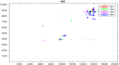
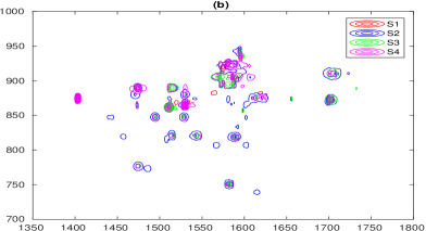
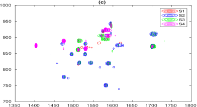
Figure 1: Contourplot of 2D HSCQ sources Limonene ($S_{1}$), Nerol ($S_{2}$), Terpinolene ($S_{3}$) and Caryophyllene ($S_{4}$). (a) pure sources, (b) (resp.(c)) estimated sources using the $\ell_{1}$ norm (resp. the $\beta$-divergence with the $\operatorname{\textbf{Ent}}$ regularization function).

References

- [1] P. Comon and C. Jutten. Handbook of Blind Source Separation: Independent component analysis and applications. Academic press, 2010.
- [2] D.-D Lee and H.-S Seung. Learning the parts of objects by non-negative matrix factorization. Nature, 401(6755):788, 1999.
- [3] P. Paatero and U. Tapper. Positive matrix factorization: A non-negative factor model with optimal utilization of error estimates of data values. Environmetrics, 5(2):111–126, 1994.
- [4] C. Févotte, N. Bertin, and J.-L. Durrieu. Nonnegative matrix factorization with the Itakura-Saito divergence: With application to music analysis. Neural computation, 21(3):793–830, 2009.
- [5] C. Févotte and J. Idier. Algorithms for nonnegative matrix factorization with the -divergence. Neural computation, 23(9):2421–2456, 2011.
- [6] A. Cherni, E. Piersanti, and C. Chaux. NMF-based sparse unmixing of complex mixtures. In SPARS workshop, Toulouse, France, Jul. 2019.
- [7] R. Kompass. A generalized divergence measure for nonnegative matrix factorization. Neural computation, 19(3):780–791, 2007.
- [8] A. Basu, I.-R Harris, N.-L Hjort, and M.-C Jones. Robust and efficient estimation by minimising a density power divergence. Biometrika, 85(3):549–559, 1998.
- [9] T. Hoffman. Probabilistic latent semantic indexing. In Proceedings of the 22nd Annual ACM Conference on Research and Development in Information Retrieval, pages 50–57, 1999.
- [10] E. J. Candes and M. B. Wakin. An introduction to compressive sampling. IEEE Signal Processing Magazine, 25(2):21–30, March 2008.
- [11] A. Beck and M. Teboulle. A fast iterative shrinkage-thresholding algorithm for linear inverse problems. SIAM Journal on Imaging Sciences, 2(1):183–202, 2009.
- [12] A. Cherni, E. Chouzenoux, and M.-A Delsuc. Proximity operators for a class of hybrid sparsity+ entropy priors application to dosy NMR signal reconstruction. In 2016 International Symposium on Signal, Image, Video and Communications (ISIVC), pages 120–125. IEEE, 2016.
- [13] A. Cherni, E. Chouzenoux, and M.-A Delsuc. PALMA, an improved algorithm for dosy signal processing. Analyst, 142(5):772–779, 2017.
- [14] D.-R Hunter and K. Lange. Rejoinder. Journal of Computational and Graphical Statistics, 9(1):52–59, 2000.
- [15] R.-M. Corless, G.-H. Gonnet, D.-E. Hare, D.-J. Jeffrey, and D.-E. Knuth. On the lambert W function. Advances in Applied Mathematics, 5(1):329–359, 1996.
- [16] E. Chouzenoux, J.-C. Pesquet, and A. Repetti. Variable metric forward–backward algorithm for minimizing the sum of a differentiable function and a convex function. Journal of Optimization Theory and Applications, 162(1):107–132, 2014.
- [17] A. Cherni, E. Piersanti, S. Anthoine, C. Chaux, L. Shintu, M. Yemloul, and B. Torrésani. Challenges in the decomposition of 2D NMR spectra of mixtures of small molecules. Faraday discussions, 218:459–480, 2019.
- [18] J.-F. Cardoso and A. Souloumiac. Blind beamforming for non-gaussian signals. IEE Proceedings F - Radar and Signal Processing, 140(6):362–370, 1993.
- [19] E. Vincent, R. Gribonval, and C. Févotte. Performance measurement in blind audio source separation. IEEE transactions on audio, speech, and language processing, 14(4):1462–1469, 2006.
- [20] E. Moreau and O. Macchi. A one stage self-adaptive algorithm for source separation. In Proceedings of ICASSP 94. IEEE International Conference on Acoustics, Speech and Signal Processing, volume 3, pages III–49. IEEE, 1994.