Jeans mass-radius relation of self-gravitating Bose-Einstein condensates and
typical parameters of the dark matter particle

Abstract

We study the Jeans mass-radius relation of Bose-Einstein condensate dark matter in Newtonian gravity. We show at a general level that it is similar to the mass-radius relation of Bose-Einstein condensate dark matter halos [P.H. Chavanis, Phys. Rev. D 84, 043531 (2011)]. Bosons with a repulsive self-interaction generically evolve from the Thomas-Fermi regime to the noninteracting regime as the Universe expands. In the Thomas-Fermi regime, the Jeans radius remains approximately constant while the Jeans mass decreases. In the noninteracting regime, the Jeans radius increases while the Jeans mass decreases. Bosons with an attractive self-interaction generically evolve from the nongravitational regime to the noninteracting regime as the Universe expands. In the nongravitational regime, the Jeans radius and the Jeans mass increase. In the noninteracting regime, the Jeans radius increases while the Jeans mass decreases. The transition occurs at a maximum Jeans mass which is similar to the maximum mass of Bose-Einstein condensate dark matter halos with an attractive self-interaction. We use the mass-radius relation of dark matter halos and the observational evidence of a “minimum halo” (with typical radius $R\sim 1\,{\rm kpc}$ and typical mass $M\sim 10^{8}\,M_{\odot}$) to constrain the mass $m$ and the scattering length $a_{s}$ of the dark matter particle. For noninteracting bosons, $m$ is of the order of $2.92\times 10^{-22}\,{\rm eV}/c^{2}$. The mass of bosons with an attractive self-interaction can only be slightly smaller ($2.19\times 10^{-22}\,{\rm eV}/c^{2}<m<2.92\times 10^{-22}\,{\rm eV}/c^{2}$ and $-1.11\times 10^{-62}\,{\rm fm}\leq a_{s}\leq 0$) otherwise the minimum halo would be unstable. Constraints from particle physics and cosmology imply $m=2.92\times 10^{-22}\,{\rm eV}/c^{2}$ and $a_{s}=-3.18\times 10^{-68}\,{\rm fm}$ for ultralight axions and it is then found that attractive self-interactions can be neglected both in the linear and nonlinear regimes of structure formation. The mass of bosons with a repulsive self-interaction can be larger by $18$ orders of magnitude ($2.92\times 10^{-22}\,{\rm eV}/c^{2}<m<1.10\times 10^{-3}\,{\rm eV}/c^{2}$ and $0\leq a_{s}\leq 4.41\times 10^{-6}\,{\rm fm}$). The maximum allowed mass ($m=1.10\times 10^{-3}\,{\rm eV}/c^{2}$ and $a_{s}=4.41\times 10^{-6}\,{\rm fm}$) is determined by the Bullet Cluster constraint while the transition between the noninteracting limit and the Thomas-Fermi limit corresponds to $m=2.92\times 10^{-22}\,{\rm eV}/c^{2}$ and $a_{s}=8.13\times 10^{-62}\,{\rm fm}$. For each of these models, we calculate the Jeans length and the Jeans mass at the epoch of radiation-matter equality and at the present epoch.

I Introduction

Even after $100$ years of research, the nature of dark matter (DM) is still elusive. The standard cold dark matter (CDM) model, in which DM is represented by a classical pressureless fluid at zero temperature ($T=0$) or by a collisionless $N$-body system of classical particles, works extremely well at large (cosmological) scales and can account for precise measurements of the cosmic microwave background (CMB) from WMAP and Planck missions planck2013 ; planck2016 . However, in addition to the lack of evidence for any CDM particle such as a weakly interacting massive particle (WIMP) with a mass in the GeV-TeV range, the CDM model faces serious problems at small (galactic) scales that are known as the “core-cusp” problem moore , the “missing satellites” problem satellites1 ; satellites2 ; satellites3 , and the “too big to fail” problem boylan . This “small-scale crisis of CDM” crisis is somehow related to the assumption that DM is pressureless implying that gravitational collapse takes place at all scales. A possibility to solve these problems is to consider self-interacting dark matter (SIDM) spergelsteinhardt , warm dark matter (WDM) wdm , or the feedback of baryons that can transform cusps into cores romano1 ; romano2 ; romano3 . Another promising possibility to solve the CDM crisis is to take into account the quantum (or wave) nature of the DM particle. Indeed, in quantum mechanics, an effective pressure is present even at $T=0$. This quantum pressure may balance the gravitational attraction at small scales and solve the CDM crisis.

In this paper, we shall consider the possibility that the DM particle is a boson, e.g., an ultralight axion (ULA) marshrevue . At $T=0$, bosons form Bose-Einstein condensates (BECs) and they are described by a single wavefunction $\psi({\bf r},t)$. They can therefore be interpreted as a scalar field (SF). The bosons may be noninteracting or may have a repulsive or an attractive self-interaction (for example, the QCD axion has an attractive self-interaction). On astrophysical scales, one must generally take into account gravitational interactions between the bosons. The evolution of the wave function of self-gravitating BECs is then governed by the Schrödinger-Poisson (SP) equations when the bosons are noninteracting or by the Gross-Pitaevskii-Poisson (GPP) equations when the bosons are self-interacting. BECDM halos can thus be viewed as gigantic bosonic atoms where the bosonic particles are condensed in a single macroscopic quantum state. The wave properties of the SF are negligible at large (cosmological) scales where the SF behaves as CDM, but they become important at small (galactic) scales where they can prevent gravitational collapse, providing halo cores and suppressing small-scale structures. This model has been given several names such as wave DM, fuzzy dark matter (FDM), BECDM, $\psi$DM, or SFDM baldeschi ; khlopov ; membrado ; maps ; bianchi ; sin ; jisin ; leekoh ; schunckpreprint ; matosguzman ; sahni ; guzmanmatos ; hu ; peebles ; goodman ; mu ; arbey1 ; silverman1 ; matosall ; silverman ; lesgourgues ; arbey ; fm1 ; bohmer ; fm2 ; bmn ; fm3 ; sikivie ; mvm ; lee09 ; ch1 ; lee ; prd1 ; prd2 ; prd3 ; briscese ; harkocosmo ; harko ; abrilMNRAS ; aacosmo ; velten ; pires ; park ; rmbec ; rindler ; lora2 ; abrilJCAP ; mhh ; lensing ; glgr1 ; ch2 ; ch3 ; shapiro ; bettoni ; lora ; mlbec ; madarassy ; marsh ; abrilph ; playa ; stiff ; souza ; freitas ; alexandre ; schroven ; pop ; cembranos ; schwabe ; fan ; calabrese ; bectcoll ; chavmatos ; hui ; abrilphas ; ggpp ; shapironew ; mocz ; zhang ; suarezchavanisprd3 ; veltmaat ; moczSV ; phi6 ; bbbs ; cmnjv ; psgkk ; ekhe ; matosbh ; tkachevprl2 ; epjpbh ; ag ; lhb ; nmibv ; zlc ; bm ; modeldm ; bft ; bblp ; dn ; bbes ; bvc ; moczamin ; mabc ; gga ; moczprl ; mcmh ; harkoj ; mcmhbh ; reig ; dm ; adgltt ; moczmnras ; verma ; braxbh ; lancaster ; tunnel (see the Introduction of prd1 and Ref. leerevue for an early history of this model and Refs. srm ; rds ; chavanisbook ; marshrevue ; niemeyer ; ferreira for reviews). Here, we shall use the name BECDM. In the BECDM model, gravitational collapse is prevented by the quantum pressure arising from the Heisenberg uncertainty principle or from the scattering of the bosons (when the self-interaction is repulsive). Therefore, quantum mechanics (or a repulsive self-interaction) may solve the small-scale problems of the CDM model mentioned above.

It is usually considered that large-scale structures such as galaxies or dark matter halos form in a homogeneous universe by Jeans instability jeans1902 . For a cold classical gas, the Jeans length vanishes or is extremely small ($\lambda_{J}\simeq 0$) implying that structures can form at all scales. This is not what we observe and this leads to the CDM crisis. By contrast, when quantum mechanics (or a repulsive self-interaction) is taken into account, the Jeans length is non-zero implying the absence of structures below a minimum scale in agreement with the observations. The Jeans instability of a self-gravitating BEC with repulsive or attractive self-interaction was first considered by Khlopov et al. khlopov and Bianchi et al. bianchi in a general relativistic framework based on the Klein-Gordon-Einstein equations. The Jeans instability of a noninteracting self-gravitating BEC in Newtonian gravity described by the SP equations was studied by Hu et al. hu and Sikivie and Yang sikivie . Finally, the Jeans instability of a Newtonian self-gravitating BEC with repulsive or attractive self-interactions described by the GPP equations was studied by Chavanis prd1 . These results were extended in general relativity by Suárez and Chavanis suarezchavanisprd3 going beyond some of the approximations made by Khlopov et al. khlopov (see footnote 7 of suarezchavanisprd3 ). Recently, Harko harkoj considered the Jeans instability of rotating Newtonian BECs in the TF limit. In these different studies, the authors determined the Jeans length and the Jeans mass of the BECs and used them to obtain an estimate of the minimum size and minimum length of BECDM halos.

The Jeans instability study is only valid in the linear regime of structure formation. It describes the initiation of the large-scale structures of the Universe. The Jeans instability leads to a growth of the perturbations and the formation of condensations (clumps). When the density contrast reaches a sufficiently large value, the condensations experience a free fall, followed by a complicated process of gravitational cooling and violent relaxation. They can also undergo merging and accretion. This corresponds to the nonlinear regime of structure formation leading to DM halos. BECDM halos result from the balance between the gravitational attraction and the quantum pressure due to the Heisenberg principle and the self-interaction of the bosons. Observations reveal that, contrary to the prediction of the CDM model, there are no halos with a mass smaller than $M\sim 10^{8}\,M_{\odot}$ and with a size smaller than $R\sim 1\,{\rm kpc}$. These ultracompact DM halos correspond typically to dwarf spheroidal galaxies (dSphs) like Fornax. To be specific, we shall assume that Fornax is the smallest halo observed in the Universe. In the BECDM model, this “minimum halo” is interpreted as the ground state of the self-gravitating BEC at $T=0$. Bigger halos have a core-halo structure with a quantum core (ground state) surrounded by an approximately isothermal atmosphere which results from quantum interferences. This core-halo structure is observed in numerical simulations of BECDM ch2 ; ch3 ; schwabe ; mocz ; moczSV ; veltmaat ; moczprl ; moczmnras . The quantum core may solve the small-scale problems of the CDM model such as the cusp problem and the missing satellite problem. The approximately isothermal atmosphere is consistent with the classical NFW profile and accounts for the flat rotation curves of the galaxies at large distances. The mass-radius relation of BECDM halos at $T=0$ (ground state) representing the minimum halo or the quantum core of larger halos has been determined in Refs. prd1 ; prd2 for bosons with vanishing, repulsive, or attractive self-interaction. It can be obtained either numerically prd2 by solving the GPP equations or analytically prd1 by using a gaussian ansatz for the wavefunction. The quantum core mass – halo mass relation $M_{c}(M_{h})$ was first obtained by Schive et al. ch3 , in the case of noninteracting bosons, from direct numerical simulations and heuristic arguments. This relation was later derived in Refs. modeldm ; mcmh ; mcmhbh from an effective thermodynamic approach by maximizing the entropy at fixed mass and energy. It was also extended to the case of self-interacting bosons (with a repulsive of an attractive self-interaction) and fermions modeldm ; mcmh ; mcmhbh .

It was noticed in Ref. prd1 that the Jeans mass-radius relation obtained from the dispersion relation of self-gravitating homogeneous BECs is similar to the mass-radius relation of BECDM halos obtained by solving the equation of quantum hydrostatic equilibrium with a Gaussian ansatz. This agreement is surprising because the two relations apply to very different regimes of structure formation: linear versus nonlinear. It results, however, essentially from dimensional analysis. The aim of the present paper is to further develop this analogy and study its consequences. In Sec. II we recall the basic equations describing self-gravitating BECs. Using the Madelung madelung transformation, we write the GPP equations in the form of hydrodynamic equations. We then consider spatially inhomogeneous solutions of these equations representing BECDM halos. They correspond to stationary solutions of the GPP equations or to stationary solutions of the quantum Euler-Poisson equations satisfying the condition of hydrostatic equilibrium. Stable equilibrium states follow a minimum energy principle. We also consider the Jeans instability of an infinite homogeneous self-gravitating BEC. We recall the general dispersion relation and the Jeans wavenumber obtained in Ref. prd1 from which we can obtain the Jeans length and the Jeans mass. We briefly discuss the Jeans instability in an expanding universe. In Sec. III we derive the analytical mass-radius relation of BECDM halos from a general ansatz on the wavefunction ($f$-ansatz). We determine the parameters of this relation by comparing its asymptotic limits with the exact results obtained by solving the GPP equations numerically prd2 . In this manner, the analytical mass-radius relation that we obtain provides a very good agreement with the exact numerical mass-radius relation. In Sec. IV, we use the fact that this mass-radius relation applies to the minimum halo (with $R\sim 1\,{\rm kpc}$ and $M\sim 10^{8}\,M_{\odot}$) to obtain the dark matter particle mass-scattering length relation. This is a constraint that the parameters of the DM particle must satisfy in order to reproduce the characteristics of the minimum halo (assumed to correspond to the ground state of the BECDM model). Using additional constraints such as the Bullet Cluster constraint, or constraints from particle physics and cosmology, we can put some bounds on the possible values of $m$ and $a_{s}$. We consider specific models of physical interest that we call BECNI, BECTF, BECt, BECcrit and BECth. Once the values of $m$ and $a_{s}$ have been determined from the previous considerations, we study in Sec. V the evolution of the Jeans radius and Jeans mass as a function of the cosmic density, as the Universe expands. We confirm that the Jeans mass-radius relation is similar to the mass-radius relation of DM halos, the density of the universe playing in this analogy the role of the average density of DM halos. We characterize different regimes (noninteracting, TF, nongravitational) for bosons with repulsive or attractive self-interaction. Finally, we explain how our results can be extended to more general forms of self-interaction.

II Self-gravitating Bose-Einstein condensates

II.1 Gross-Pitaevskii-Poisson equations

We assume that DM is made of bosons (like the axion) in the form of BECs at $T=0$. We use a nonrelativistic approach based on Newtonian gravity. The evolution of the wave function $\psi({\bf r},t)$ of a self-gravitating BEC is governed by the Gross-Pitaevskii-Poisson (GPP) equations (see, e.g., prd1 )

$$i\hbar\frac{\partial\psi}{\partial t}=-\frac{\hbar^{2}}{2m}\Delta\psi+m\frac{dV}{d|\psi|^{2}}\psi+m\Phi\psi,$$ (1)

$$\Delta\Phi=4\pi G|\psi|^{2},$$ (2)

where $\Phi({\bf r},t)$ is the gravitational potential and $m$ is the mass of the bosons. The first term in Eq. (1) is the kinetic term which accounts for the Heisenberg uncertainty principle. The second term takes into account the self-interaction of the bosons via a potential $V(|\psi|^{2})$. The third term accounts for the self-gravity of the BEC. The mass density of the BEC is $\rho({\bf r},t)=|\psi|^{2}$.

For the standard BEC, we have

$$V(|\psi|^{2})=\frac{2\pi a_{s}\hbar^{2}}{m^{3}}|\psi|^{4},$$ (3)

where $a_{s}$ is the scattering length of the bosons. The interaction between the bosons is repulsive when $a_{s}>0$ and attractive when $a_{s}<0$. This potential is valid provided that the gas is sufficiently dilute. It corresponds to a power-law potential of the form

$$V(|\psi|^{2})=\frac{K}{\gamma-1}|\psi|^{2\gamma}$$ (4)

with

$$\gamma=2\quad{\rm and}\quad K=\frac{2\pi a_{s}\hbar^{2}}{m^{3}}.$$ (5)

The GPP equations conserve the mass

$$M=\int|\psi|^{2}\,d{\bf r}$$ (6)

and the energy

$$E_{\rm tot}=\frac{\hbar^{2}}{2m^{2}}\int|\nabla\psi|^{2}\,d{\bf r}+\int V(|\psi|^{2})\,d{\bf r}+\frac{1}{2}\int|\psi|^{2}\Phi\,d{\bf r},$$ (7)

which is the sum of the kinetic energy $\Theta$, the internal energy $U$, and the gravitational energy $W$ (i.e. $E_{\rm tot}=\Theta+U+W$).

Remark: the GPP equations (1) and (2) may be obtained from the KGE equations in the nonrelativistic limit $c\rightarrow+\infty$ for a SF interacting via a potential $V_{R}(\varphi)$ (see, e.g., playa ; chavmatos for a complex SF and phi6 ; tunnel for a real SF).

II.2 The Madelung transformation

Writing the wave function as

$$\psi({\bf r},t)=\sqrt{{\rho({\bf r},t)}}e^{iS({\bf r},t)/\hbar},$$ (8)

where $\rho({\bf r},t)$ is the mass density and $S({\bf r},t)$ is the action, and making the Madelung madelung transformation

$$\rho({\bf r},t)=|\psi|^{2}\qquad{\rm and}\qquad{\bf u}=\frac{\nabla S}{m},$$ (9)

where ${\bf u}({\bf r},t)$ is the velocity field, the GPP equations (1) and (2) can be written under the form of hydrodynamic equations

$$\frac{\partial\rho}{\partial t}+\nabla\cdot(\rho{\bf u})=0,$$ (10)

$$\frac{\partial S}{\partial t}+\frac{(\nabla S)^{2}}{2m}+m\left[\Phi+V^{\prime}(\rho)\right]+Q=0,$$ (11)

$$\frac{\partial{\bf u}}{\partial t}+({\bf u}\cdot\nabla){\bf u}=-\frac{1}{m}\nabla Q-\frac{1}{\rho}\nabla P-\nabla\Phi,$$ (12)

$$\Delta\Phi=4\pi G\rho,$$ (13)

where

$$Q=-\frac{\hbar^{2}}{2m}\frac{\Delta\sqrt{\rho}}{\sqrt{\rho}}=-\frac{\hbar^{2}}{4m}\left[\frac{\Delta\rho}{\rho}-\frac{1}{2}\frac{(\nabla\rho)^{2}}{\rho^{2}}\right]$$ (14)

is the quantum potential which takes into account the Heisenberg uncertainty principle. On the other hand, the pressure $P$ is a function $P({\bf r},t)=P[\rho({\bf r},t)]$ of the density (the fluid is barotropic) which is determined by the potential $V(\rho)$ through the relation

$$P(\rho)=\rho V^{\prime}(\rho)-V(\rho)=\rho^{2}\left[\frac{V(\rho)}{\rho}\right]^{\prime}$$ (15)

equivalent to

$$P^{\prime}(\rho)=\rho V^{\prime\prime}(\rho).$$ (16)

The speed of sound $c_{s}$ is given by

$$c_{s}^{2}=P^{\prime}(\rho)=\rho V^{\prime\prime}(\rho).$$ (17)

For a power-law potential of the form of Eq. (4), we get a polytropic equation of state

$$V(\rho)=\frac{K}{\gamma-1}\rho^{\gamma}\quad \Rightarrow \quad P=K\rho^{\gamma}$$ (18)

$$\Rightarrow \quad c_{s}^{2}=K\gamma\rho^{\gamma-1}.$$

In particular, for the standard BEC, we obtain

$$V(\rho)=\frac{2\pi a_{s}\hbar^{2}}{m^{3}}\rho^{2}\quad \Rightarrow \quad P=\frac{2\pi a_{s}\hbar^{2}}{m^{3}}\rho^{2}$$ (19)

$$\Rightarrow \quad c_{s}^{2}=\frac{4\pi a_{s}\hbar^{2}}{m^{3}}\rho.$$

The equation of state is quadratic. The hydrodynamic equations (10)-(13) are called the quantum Euler-Poisson equations prd1 . Equation (11) is the quantum Hamilton-Jacobi (or Bernoulli) equation. In the TF limit where the quantum potential can be neglected (formally $\hbar=0$), they become equivalent to the classical Euler-Poisson equations for a barotropic gas bt .

The quantum Euler equations conserve the mass

$$M=\int\rho\,d{\bf r}$$ (20)

and the energy (see, e.g., prd1 )

$$E_{\rm tot}=\Theta_{c}+\Theta_{Q}+U+W,$$ (21)

which is the sum of the classical kinetic energy

$$\Theta_{c}=\int\rho\frac{{\bf u}^{2}}{2}\,d{\bf r},$$ (22)

the quantum kinetic energy

$$\Theta_{Q}=\frac{\hbar^{2}}{8m^{2}}\int\frac{(\nabla\rho)^{2}}{\rho}\,d{\bf r}=\frac{1}{m}\int\rho Q\,d{\bf r},$$ (23)

the internal energy

$$U=\int V(\rho)\,d{\bf r}=\int\rho\int^{\rho}\frac{P(\rho^{\prime})}{{\rho^{\prime}}^{2}}\,d\rho^{\prime}\,d{\bf r},$$ (24)

and the gravitational energy

$$W=\frac{1}{2}\int\rho\Phi\,d{\bf r}.$$ (25)

At equilibrium, the classical (macroscopic) kinetic energy vanishes and we get

$$E_{\rm tot}=\Theta_{Q}+U+W.$$ (26)

The quantum virial theorem writes (see, e.g., prd1 ; ggpp )

$$\frac{1}{2}\ddot{I}=2(\Theta_{c}+\Theta_{Q})+3\int P\,d{\bf r}+W,$$ (27)

where

$$I=\int\rho r^{2}\,d{\bf r}$$ (28)

is the moment of inertia. At equilibrium, it reduces to

$$2\Theta_{Q}+3\int P\,d{\bf r}+W=0.$$ (29)

For a polytropic equation of state $P=K\rho^{\gamma}$, we have $\int P\,d{\bf r}=(\gamma-1)U$ and the equilibrium virial theorem may be written as $2\Theta_{Q}+3(\gamma-1)U+W=0$. In particular, for the standard BEC for which $\gamma=2$, we have $\int P\,d{\bf r}=U$ and the equilibrium virial theorem reduces to $2\Theta_{Q}+3U+W=0$.

By using the Madelung transformation, the GPP equations (1) and (2) have be written in the form of hydrodynamic equations involving a quantum potential taking into account the Heisenberg uncertainty principle and a pressure force arising from the self-interaction of the bosons. This transformation allows us to treat the BEC as a quantum fluid (superfluid) and to apply standard methods developed in astrophysics as discussed below.

Remark: The GPP equations (1) and (2) and the quantum Euler-Poisson equations (10)-(13) can be written in terms of the functional derivative of the total energy $E_{\rm tot}$ (see Sec. 3.6 of ggpp ). They can also be obtained from a least action principle and a Lagrangian (see Appendix B of bectcoll and Appendix F of ggpp ).

II.3 Spatially inhomogeneous equilibrium states in the nonlinear regime: BECDM halos

We first apply the GPP equations (1) and (2), or equivalently the quantum Euler-Poisson equations (10)-(13), to BECDM halos that appear in the nonlinear regime of structure formation in cosmology.

A stationary solution of GPP equations is of the form

$$\psi({\bf r},t)=\phi({\bf r})e^{-iEt/\hbar},$$ (30)

where $\phi({\bf r})=\sqrt{\rho({\bf r})}$ and $E$ are real. Substituting Eq. (30) into Eqs. (1) and (2), we obtain the eigenvalue problem

$$-\frac{\hbar^{2}}{2m}\Delta\phi+m\frac{dV}{d\phi^{2}}\phi+m\Phi\phi=E\phi,$$ (31)

$$\Delta\phi=4\pi G\phi^{2},$$ (32)

determining the eigenfunctions $\phi({\bf r})$ and the eigenvalues $E$. For the fundamental mode (the one with the lowest energy) the wavefunction $\phi(r)$ is spherically symmetric and has no node so that the density profile decreases monotonically with the radial distance. Dividing Eq. (31) by $\phi$ and using $\rho=\phi^{2}$, we obtain the identity

$$Q+mV^{\prime}(\rho)+m\Phi=E,$$ (33)

which can also be obtained from the quantum Hamilton-Jacobi (or Bernoulli) equation (11) with $S=-Et$. Multiplying Eq. (33) by $\rho/m$ and integrating over the system we get

$$NE=\Theta_{Q}+\int\rho V^{\prime}(\rho)\,d{\bf r}+2W.$$ (34)

For a polytropic equation of state $P=K\rho^{\gamma}$, we have $\int\rho V^{\prime}(\rho)\,d{\bf r}=\gamma U$ and Eq. (34) may be written as $NE=\Theta_{Q}+\gamma U+2W$. In particular, for the standard BEC for which $\gamma=2$, we get $\int\rho V^{\prime}(\rho)\,d{\bf r}=2U$ and Eq. (34) reduces to $NE=\Theta_{Q}+2U+2W$.

Equivalent results can be obtained from the hydrodynamic equations (10)-(13). Indeed, the condition of quantum hydrostatic equilibrium, corresponding to a steady state of the quantum Euler equation (12), writes

$$\frac{\rho}{m}\nabla Q+\nabla P+\rho\nabla\Phi={\bf 0}.$$ (35)

Dividing Eq. (35) by $\rho$ and integrating the resulting expression with the help of Eq. (16), we recover Eq. (33) where $E$ appears as a constant of integration. On the other hand, combining Eq. (35) with the Poisson equation (13), we obtain the fundamental differential equation of quantum hydrostatic equilibrium

$$\frac{\hbar^{2}}{2m^{2}}\Delta\left(\frac{\Delta\sqrt{\rho}}{\sqrt{\rho}}\right)-\nabla\cdot\left(\frac{\nabla P}{\rho}\right)=4\pi G\rho.$$ (36)

This equation describes the balance between the quantum potential taking into account the Heisenberg uncertainty principle, the pressure due to the self-interaction of the bosons, and the self-gravity. For the standard BEC, using Eq. (19), it takes the form

$$\frac{\hbar^{2}}{2m^{2}}\Delta\left(\frac{\Delta\sqrt{\rho}}{\sqrt{\rho}}\right)-\frac{4\pi a_{s}\hbar^{2}}{m^{3}}\Delta\rho=4\pi G\rho.$$ (37)

These results can also be obtained from an energy principle (see Appendix B). Indeed, one can show that an equilibrium state of the GPP equations is an extremum of energy $E_{\rm tot}$ at fixed mass $M$ and that an equilibrium state is stable if, and only if, it is a minimum of energy at fixed mass. We are led therefore to considering the minimization problem

$$\min\quad\{E_{\rm tot}\quad|\quad M\quad{\rm fixed}\}.$$ (38)

Writing the variational problem for the first variations (extremization problem) as

$$\delta E_{\rm tot}-\frac{\mu}{m}\delta M=0,$$ (39)

where $\mu$ (global chemical potential) is a Lagrange multiplier taking into account the mass constraint, we obtain ${\bf u}={\bf 0}$ and

$$Q+mV^{\prime}(\rho)+m\Phi=\mu.$$ (40)

This relation is equivalent to Eq. (33) provided that we make the identification $E=\mu$. Therefore, the eigenenergy $E$ coincides with the global chemical potential $\mu$. Eq. (40) is also equivalent to the condition of quantum hydrostatic equilibrium (35). Therefore, an extremum of energy at fixed mass is an equilibrium state of the GPP equations. Furthermore, as shown in Appendix B, among all possible equilibria, only minima of energy at fixed mass are dynamically stable with respect to the GPP equations (maxima or saddle points are linearly unstable). The stability of an equilibrium state can be settled by studying the sign of $\delta^{2}E_{\rm tot}$ or, equivalently, by linearizing the equations of motion about the equilibrium state and investigating the sign of the square pulsation $\omega^{2}$ (see Appendix B). In each case, these methods require to solve a rather complicated eigenvalue equation. Alternatively, the stability of an equilibrium state can be settled more directly by plotting the series of equilibria and using the Poincaré-Katz poincare ; katzpoincare turning point criterion applied on the curve $\mu(M)$ or the Wheeler htww theorem applied on the curve $M(R)$ (see prd1 ; prd2 ; phi6 for a specific application of these methods to the case of axion stars). It may also be useful to plot the curve $E_{\rm tot}(M)$ in order to compare the energy of different equilibrium states with the same mass $M$. Since $\delta M=0\Leftrightarrow\delta E_{\rm tot}=0$ according to Eq. (39), the extrema of mass coincide with the extrema of energy in the series of equilibria. As a result, the curve $E_{\rm tot}(M)$ presents cusps at these critical points (see, e.g., Fig. 11 of prd2 for illustration).

The fundamental equation of hydrostatic equilibrium of BECDM halos, Eq. (37), has been solved analytically (using a Gaussian ansatz) in prd1 , and numerically in prd2 , for an arbitrary self-interaction (repulsive or attractive). It describes a compact quantum object (soliton/BEC). Because of quantum effects, the central density is finite instead of diverging as in the CDM model. Therefore, quantum mechanics is able to solve the cusp-core problem.

For noninteracting bosons ($a_{s}=0$), Eq. (37) reduces to

$$\frac{\hbar^{2}}{2m^{2}}\Delta\left(\frac{\Delta\sqrt{\rho}}{\sqrt{\rho}}\right)=4\pi G\rho.$$ (41)

The density profile is plotted in Fig. 2 of mcmh using the results of prd2 . The density has not a compact support: the density decreases to zero at infinity exponentially rapidly. The mass-radius relation is given by membrado ; prd2

$$M=9.95\frac{\hbar^{2}}{Gm^{2}R_{99}},$$ (42)

where $R_{99}$ represents the radius containing $99\%$ of the mass. The mass decreases as the radius increases. The equilibrium states are all stable.

For bosons with a repulsive self-interaction ($a_{s}>0$), some density profiles are plotted in prd2 . The density has not a compact support except in the TF limit (see below). The mass-radius relation is plotted in Fig. 4 of prd2 (see also Fig. 2 below). There is a minimum radius (see Eq. (45) below) reached for $M\rightarrow+\infty$. The mass decreases as the radius increases. The equilibrium states are all stable. In the TF limit, Eq. (37) reduces to

$$\frac{4\pi a_{s}\hbar^{2}}{m^{3}}\Delta\rho+4\pi G\rho=0.$$ (43)

This equation is equivalent to the Lane-Emden equation for a polytrope of index $n=1$ chandra . It has a simple analytical solution

$$\rho=\frac{\rho_{0}R}{\pi r}\sin\left(\frac{\pi r}{R_{\rm TF}}\right).$$ (44)

The density profile is plotted in Fig. 3 of mcmh . In the TF limit, the density has a compact support: the density vanishes at a finite radius $R_{\rm TF}$. The equilibrium states have a unique radius given by tkachev ; maps ; leekoh ; goodman ; arbey ; bohmer ; prd1

$$R_{\rm TF}=\pi\left(\frac{a_{s}\hbar^{2}}{Gm^{3}}\right)^{1/2},$$ (45)

independent of their mass $M$. In the noninteracting (NI) limit $R\gg R_{\rm TF}$, we recover Eq. (42).

Figure 1: Density profile of a self-gravitating BEC with an attractive self-interaction at the maximum mass $M_{\rm max}$. We have adopted the values $m=2.19\times 10^{-22}\,{\rm eV}/c^{2}$ and $a_{s}=-1.11\times 10^{-62}\,{\rm fm}$ (see Sec. III.3) corresponding to a DM halo of mass $M=10^{8}\,M_{\odot}$ and radius $R=1\,{\rm kpc}$ (minimum halo).

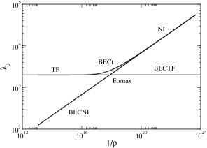
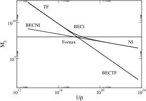
Figure 6: Evolution of the Jeans length and Jeans mass with the inverse density of the universe for bosons with a repulsive self-interaction ($\lambda_{J}$ is in ${\rm pc}$, $M_{J}$ is in solar masses $M_{\odot}$, and $\rho$ is in ${\rm g/m^{3}}$) for the three models BECNI, BECTF and BECt considered in the text. Here and in the following figures we have indicated the values $\lambda_{J}/2=1\,{\rm kpc}$, $M_{J}=10^{8}\,M_{\odot}$ and $\rho=1.62\times 10^{-18}\,{\rm g/m^{3}}$ corresponding to the minimum halo (Fornax) for reference (see Sec. V.6).

For bosons with an attractive self-interaction ($a_{s}<0$), some density profiles are plotted in prd2 . The density has not a compact support. The mass-radius relation is plotted in Fig. 6 of prd2 (see also Fig. 3 below). There is a maximum mass prd1 ; prd2

$$M_{\rm max}=1.012\,\frac{\hbar}{\sqrt{Gm|a_{s}|}}$$ (46)

at

$$R_{99}^{*}=5.5\,\left(\frac{|a_{s}|\hbar^{2}}{Gm^{3}}\right)^{1/2}.$$ (47)

The density profile at the maximum mass is plotted in Fig. 1 using the results of prd2 . There is no equilibrium state with $M>M_{\rm max}$. In that case, the BEC is expected to collapse bectcoll . The outcome of the collapse (dense axion star, black hole, bosenova…) is discussed in braaten ; cotner ; bectcoll ; ebycollapse ; tkachevprl ; helfer ; phi6 ; visinelli ; moss . For $M<M_{\rm max}$ the equilibrium states with $R>R_{99}^{*}$ are stable and the equilibrium states with $R<R_{99}^{*}$ are unstable. In the nongravitational (NG) limit $R\ll R_{99}^{*}$, Eq. (37) can be written as

$$-\frac{\hbar^{2}}{2m}\frac{\Delta\sqrt{\rho}}{\sqrt{\rho}}+\frac{4\pi a_{s}\hbar^{2}}{m^{2}}\rho=E.$$ (48)

It is equivalent to the standard stationary GP equation. The mass-radius relation is given by (see, e.g., prd2 )

$$M=0.275\,\frac{mR_{99}}{|a_{s}|}.$$ (49)

These equilibrium states are unstable. In the NI limit $R\gg R_{99}^{*}$, we recover Eqs. (41) and (42). These equilibrium states are stable.

Remark: We have seen that self-gravitating BECs with an attractive self-interaction ($a_{s}<0$) can be at equilibrium only below a maximum mass given by Eq. (46). Conversely, a self-gravitating BEC of mass $M$ can be at equilibrium only if the scattering length of the bosons is above a minimum negative value prd1 ; prd2

$$(a_{s})_{\rm min}=-1.024\frac{\hbar^{2}}{GmM^{2}}.$$ (50)

II.4 Infinite homogeneous BEC in the linear regime: quantum Jeans problem

We now apply the GPP equations (1) and (2), or equivalently the quantum Euler-Poisson equations (10)-(13), to the universe as a whole in order to study the initiation of structure formation. Specifically, following prd1 , we study the linear dynamical stability of an infinite homogeneous self-gravitating BEC with density $\rho$ and velocity ${\bf u}={\bf 0}$ described by the quantum Euler-Poisson equations (10)-(13). This is a generalization of the classical Jeans problem jeans1902 to a quantum fluid.

Considering a small perturbation about an infinite homogeneous equilibrium state, making the Jeans swindle bt ; chavanisjeans , and linearizing the hydrodynamic equations (10)-(13), we obtain

$$\frac{\partial\delta}{\partial t}+\nabla\cdot{\bf u}=0,$$ (51)

$$\frac{\partial{\bf u}}{\partial t}=-c_{s}^{2}\nabla\delta-\nabla\delta\Phi+\frac{\hbar^{2}}{4m^{2}}\nabla(\Delta\delta),$$ (52)

$$\Delta\delta\Phi=4\pi G\rho\delta,$$ (53)

where $c_{s}^{2}=P^{\prime}(\rho)$ is the square of the speed of sound and $\delta({\bf r},t)=\delta\rho({\bf r},t)/\rho$ the density contrast. Taking the time derivative of Eq. (51) and the divergence of Eq. (52), and using the Poisson equation (53), we obtain a single equation for the density contrast

$$\frac{\partial^{2}\delta}{\partial t^{2}}=-\frac{\hbar^{2}}{4m^{2}}\Delta^{2}\delta+c_{s}^{2}\Delta\delta+4\pi G\rho\delta.$$ (54)

Expanding the solutions of this equation into plane waves of the form $\delta({\bf r},t)\propto{\rm exp}[i({\bf k}\cdot{\bf r}-\omega t)]$, we obtain the general dispersion relation prd1

$$\omega^{2}=\frac{\hbar^{2}k^{4}}{4m^{2}}+c_{s}^{2}k^{2}-4\pi G\rho.$$ (55)

This quantum dispersion relation may also be obtained from the gravitational Bogoliubov equations (see Appendix D of Ref. jeansuniverse ). For $\hbar=0$, we recover the classical Jeans dispersion relation. The dispersion relation (55) is studied in detail in prd1 ; suarezchavanisprd3 ; jeansuniverse . The generalized Jeans wavenumber $k_{J}$, corresponding to $\omega=0$, is determined by the quadratic equation

$$\frac{\hbar^{2}k_{J}^{4}}{4m^{2}}+c_{s}^{2}k_{J}^{2}-4\pi G\rho=0.$$ (56)

It is given by prd1

$$k_{J}^{2}=\frac{2m^{2}}{\hbar^{2}}\left(-c_{s}^{2}+\sqrt{c_{s}^{4}+\frac{4\pi G\rho\hbar^{2}}{m^{2}}}\right).$$ (57)

The Jeans length is $\lambda_{J}=2\pi/k_{J}$. The Jeans radius and the Jeans mass are defined by

$$R_{J}=\frac{\lambda_{J}}{2}=\frac{\pi}{k_{J}},\qquad M_{J}=\frac{4}{3}\pi\rho R_{J}^{3}.$$ (58)

They represent the minimum radius and the minimum mass of a fluctuation that can collapse at a given epoch. They are therefore expected to provide an order of magnitude of the minimum size and minimum mass of DM halos interpreted as self-gravitating BECs.

Extending the Jeans instability study for a self-gravitating BEC in an expanding universe, using the equations of Appendix I, we find that the evolution of the density contrast $\delta_{\bf k}(t)$ is determined by the equation aacosmo

$$\ddot{\delta}+2\frac{\dot{a}}{a}\dot{\delta}+\left(\frac{\hbar^{2}k^{4}}{4m^{2}a^{4}}+\frac{c_{s}^{2}k^{2}}{a^{2}}-4\pi G\rho_{b}\right)\delta=0.$$ (59)

This equation extends the classical Bonnor equation to a quantum gas. A detailed study of this equation has been performed in Refs. aacosmo ; suarezchavanisprd3 . In a static universe ($a=1$), writing $\delta\propto e^{-i\omega t}$, we recover the dispersion relation (55). The comoving Jeans length is $\lambda^{c}_{J}=\lambda_{J}/a$.

Remark: for the CDM model for which $\hbar=0$ and $c_{s}\simeq 0$, we find that $\lambda_{J}\simeq 0$. This implies that structures can form at all scales. This is not what is observed and this is why the BECDM model has been introduced. In that case, there is a nonzero Jeans length even at $T=0$ because of quantum effects.

III Mass-radius relation of BECDM halos from the $f$-ansatz

In Ref. prd1 , using a Gaussian ansatz for the wave function, we have obtained an approximate analytical expression of the mass-radius relation of self-gravitating BECs. In Appendix G.2, we show that the form of this relation is independent of the ansatz. Indeed, it is always given by

$$M=\frac{a\frac{\hbar^{2}}{Gm^{2}R}}{1-b^{2}\frac{a_{s}\hbar^{2}}{Gm^{3}R^{2}}},$$ (60)

where only the value of the coefficients $a$ and $b$ depends on the ansatz. Here, we shall determine the coefficients $a$ and $b$ so as to recover the exact mass-radius relation in some particular limits. Once the mass-radius relation is known, we can compute the average density of the DM halo by

$$\rho=\frac{3M}{4\pi R^{3}}.$$ (61)

Remark: With the Gaussian ansatz, we get $a_{G}^{*}=2\sigma_{G}/\nu_{G}=3.76$ and $b_{G}^{*}=(6\pi\zeta_{G}/\nu_{G})^{1/2}=1.73$, where we have used Eq. (241) with $\sigma_{G}=3/4$, $\zeta_{G}=1/(2\pi)^{3/2}$ and $\nu_{G}=1/\sqrt{2\pi}$. However, below, we shall identify the radius $R$ with $R_{99}$, not with the radius $R$ of the $f$-ansatz defined in Eq. (267). Since $R_{99}=2.38167\,R$ for the Gaussian ansatz, we obtain $a_{G}=2.38167\,a_{G}^{*}=8.96$ and $b_{G}=2.38167\,b_{G}^{*}=4.12$ to be compared with the more exact values of $a$ and $b$ found below.

III.1 Noninteracting bosons

For noninteracting bosons ($a_{s}=0$), the mass-radius relation from Eq. (60) reduces to

$$M=a\frac{\hbar^{2}}{Gm^{2}R}.$$ (62)

The mass decreases as the radius increases. If we identify $R$ with the radius $R_{99}$ containing $99\%$ of the mass and compare Eq. (62) with the exact mass-radius relation of noninteracting self-gravitating BECs from Eq. (42), we get $a=9.946$.

The average density is given by

$$\rho=\frac{3a}{4\pi}\frac{\hbar^{2}}{Gm^{2}R^{4}}=\frac{3}{4\pi a^{3}}\frac{G^{3}m^{6}M^{4}}{\hbar^{6}}.$$ (63)

The density decreases along the series of equilibria going from small radii to large radii. The equilibrium states are all stable.

III.2 Repulsive self-interaction

For bosons with a repulsive self-interaction ($a_{s}>0$), the exact mass-radius relation is represented in Fig. 2. The mass decreases as the radius increases. In the TF limit ($\hbar\rightarrow 0$ with $a_{s}\hbar^{2}\neq 0$), the mass-radius relation from Eq. (60) reduces to

$$R=b\left(\frac{a_{s}\hbar^{2}}{Gm^{3}}\right)^{1/2}.$$ (64)

The radius is independent of the mass. If we identify $R$ with the radius at which the density vanishes and compare Eq. (64) with the exact radius of self-gravitating BECs in the TF limit from Eq. (45), we get $b=\pi$. On the other hand, in the NI limit, we recover the result from Eq. (62) leading to $a=9.946$. We shall adopt these values of $a$ and $b$ in the repulsive case (see Fig. 2 for a comparison with the exact result).

Figure 2: Mass-radius relation of self-gravitating BECs with $a_{s}>0$ (full line: exact prd2 ; dotted line: Gaussian ansatz prd1 ; dashed line: fit from Eq. (60) with $a=9.946$ and $b=\pi$). The mass is normalized by $M_{a}=\hbar/\sqrt{Gma_{s}}$ and the radius by $R_{a}=(a_{s}\hbar^{2}/Gm^{3})^{1/2}$.

The average density decreases along the series of equilibria going from small radii to large radii, i.e., from the TF regime to the NI regime. In the TF regime, the average density is given by

$$\rho=\frac{3M}{4\pi b^{3}}\left(\frac{Gm^{3}}{a_{s}\hbar^{2}}\right)^{3/2}.$$ (65)

In the NI regime it is given by Eq. (63). The equilibrium states are all stable.

The transition between the TF regime and the NI regime (obtained by equating Eqs. (62) and (64)) typically occurs at

$$M_{t}=\frac{a}{b}\frac{\hbar}{\sqrt{Gma_{s}}},\quad R_{t}=b\left(\frac{a_{s}\hbar^{2}}{Gm^{3}}\right)^{1/2},\quad\rho_{t}=\frac{3a}{4\pi b^{4}}\frac{Gm^{4}}{a_{s}^{2}\hbar^{2}}.$$ (66)

We are in the TF regime when $M\gg M_{t}$ and $R\sim R_{t}$. We are in the NI regime when $M\ll M_{t}$ and $R\gg R_{t}$. Note that $R_{t}$ corresponds to the minimum radius $R_{\rm min}$ (i.e., the radius in the TF regime).

III.3 Attractive self-interaction

For bosons with an attractive self-interaction ($a_{s}<0$), the exact mass-radius relation is represented in Fig. 3. The mass increases as the radius increases, reaches a maximum value

$$M_{\rm max}=\frac{a}{2b}\frac{\hbar}{\sqrt{Gm|a_{s}|}}\qquad{\rm at}\qquad R_{*}=b\left(\frac{|a_{s}|\hbar^{2}}{Gm^{3}}\right)^{1/2},$$ (67)

and decreases. If we identify $R_{*}$ with the radius $(R_{*})_{99}$ containing $99\%$ of the mass and compare Eq. (67) with the exact values of the maximum mass and of the corresponding radius from Eqs. (46) and (47), we get $b=5.5$ and $a/2b=1.012$, leading to $a=11.1$. We shall adopt these values in the attractive case (see Fig. 3 for a comparison with the exact result). We note that the value $a=11.1$ obtained from the maximum mass is relatively close to the value $a=9.946$ obtained from the NI limit (see Sec. III.1). In the NG limit, the mass-radius relation from Eq. (60) reduces to

$$M=\frac{a}{b^{2}}\frac{mR}{|a_{s}|}.$$ (68)

The value $a/b^{2}=0.367$ obtained from the maximum mass is relatively close to the exact value $0.275$ from Eq. (49). This is a consistency check. The density decreases along the series of equilibria going from small radii to large radii, i.e., from the NG regime to the NI regime. In the NG regime, the average density is given by

$$\rho=\frac{3a}{4\pi b^{2}}\frac{m}{|a_{s}|R^{2}}=\frac{3a^{3}}{4\pi b^{6}}\frac{m^{3}}{|a_{s}|^{3}M^{2}}.$$ (69)

In the NI regime it is given by Eq. (63). The average density at the maximum mass is

$$\rho_{*}=\frac{3a}{8\pi b^{4}}\frac{Gm^{4}}{a_{s}^{2}\hbar^{2}}.$$ (70)

The equilibrium states are unstable before the turning point of mass ($R<R_{*}$) and stable after the turning point of mass ($R>R_{*}$).

Figure 3: Mass-radius relation of self-gravitating BECs with $a_{s}<0$ (full line: exact prd2 ; dotted line: Gaussian ansatz prd1 ; dashed line: fit from Eq. (60) with $a=11.1$ and $b=5.5$). The mass is normalized by $M_{a}=\hbar/\sqrt{Gm|a_{s}|}$ and the radius by $R_{a}=(|a_{s}|\hbar^{2}/Gm^{3})^{1/2}$.

The transition between the NG regime and the NI regime (obtained by equating Eqs. (62) and (68)) typically occurs at

$$M_{t}=\frac{a}{b}\frac{\hbar}{\sqrt{Gm|a_{s}|}},\,R_{t}=b\left(\frac{|a_{s}|\hbar^{2}}{Gm^{3}}\right)^{1/2},\,\rho_{t}=\frac{3a}{4\pi b^{4}}\frac{Gm^{4}}{a_{s}^{2}\hbar^{2}}.$$ (71)

These scales are similar to those corresponding to the maximum mass (we have $\rho_{t}=2\rho_{*}$, $M_{t}=2M_{\rm max}$ and $R_{t}=R_{*}$). We are in the NG regime when $M\ll M_{t}$ and $R\ll R_{t}$ but these equilibrium states are unstable. We are in the NI regime when $M\ll M_{t}$ and $R\gg R_{t}$. There is no equilibrium state of mass $M>M_{\rm max}$.

Remark: the scales (71) determining the transition between the NG regime and the NI regime in the attractive case are similar to the scales (66) determining the transition between the TF regime and the NI regime in the repulsive case provided that $a_{s}$ is replaced by $|a_{s}|$.

IV Dark matter particle mass - scattering length relation

As explained previously, in the BECDM model, the mass-radius relation (60) of a self-gravitating BEC at $T=0$ (ground state) describes the smallest halos observed in the Universe. They correspond to dSphs like Fornax. From the observations, these ultracompact DM halos have a typical radius $\sim 1\,{\rm kpc}$ and a typical mass $\sim 10^{8}\,M_{\odot}$. To fix the ideas, we shall consider a “minimum halo” of radius and mass

$$R=1\,{\rm kpc},\qquad M=10^{8}\,M_{\odot}\qquad({\rm Fornax}).$$ (72)

Its average density is

$$\rho=\frac{3M}{4\pi R^{3}}=1.62\times 10^{-18}\,{\rm g/m^{3}}\qquad({\rm Fornax}).$$ (73)

Since $R$ and $M$ are prescribed by Eq. (72), then Eq. (60) provides a relation

$$a_{s}=\frac{amR}{b^{2}M}\left(\frac{GMm^{2}R}{a\hbar^{2}}-1\right)$$ (74)

between the mass $m$ and the scattering length $a_{s}$ of the bosonic DM particle. Such a relation is necessary to obtain a minimum halo consistent with the observations. The DM particle mass-scattering length relation (74) may be written as

$$\frac{a_{s}}{a^{\prime}_{*}}=\left(\frac{m}{m_{0}}\right)^{3}-\frac{m}{m_{0}},$$ (75)

where we have introduced the scales

$$m_{0}=\left(\frac{a\hbar^{2}}{GMR}\right)^{1/2}$$ (76)

and

$$a^{\prime}_{*}=\frac{a^{3/2}}{b^{2}}\left(\frac{\hbar^{2}R}{GM^{3}}\right)^{1/2}.$$ (77)

The relation $m(a_{s})$ is plotted in Fig. 4. Taking $a=9.946$ and $b=\pi$ (see Secs. III.1 and III.2) adapted to bosons with a repulsive self-interaction (or no interaction), we get $m_{0}=2.92\times 10^{-22}\,{\rm eV}/c^{2}$ and $a^{\prime}_{*}=8.13\times 10^{-62}\,{\rm fm}$. Taking $a=11.1$ and $b=5.5$ (see Sec. III.3) adapted to bosons with an attractive self-interaction, we get $m_{0}=3.08\times 10^{-22}\,{\rm eV}/c^{2}$ and $a^{\prime}_{*}=3.12\times 10^{-62}\,{\rm fm}$.

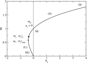
Figure 4: Mass $m$ of the DM particle as a function of the scattering length $a_{s}$ in order to match the characteristics of the minimum halo. The mass is normalized by $m_{0}$ and the scattering length by $a^{\prime}_{*}$. The stable part of the curve starts at the critical minimum halo point ($(a_{s})_{c},m_{c}$). It differs from the minimum of the curve $a_{s}(m)$.

IV.1 Noninteracting bosons

For noninteracting bosons ($a_{s}=0$), we get

$$m=m_{0}=2.92\times 10^{-22}\,{\rm eV}/c^{2}\qquad({\rm BECNI})$$ (78)

This is the typical mass considered in the literature when the bosons are assumed to be noninteracting.

Remark: In the NI regime, the mass from Eq. (78) can be written as

$$m=\left(\frac{a\hbar^{2}}{GMR}\right)^{1/2},$$ (79)

which is equivalent to Eq. (62).

IV.2 Repulsive self-interaction

For bosons with a repulsive self-interaction ($a_{s}>0$), $a^{\prime}_{*}$ determines the transition between the NI regime ($a_{s}\ll a^{\prime}_{*}$) where $m\sim m_{0}$ and the TF regime ($a_{s}\gg a^{\prime}_{*}$) where

$$\frac{m}{m_{0}}\sim\left(\frac{a_{s}}{a^{\prime}_{*}}\right)^{1/3}.$$ (80)

When the self-interaction is repulsive, we have seen that all the equilibrium states are stable. Therefore, in principle, all the scattering lengths $a_{s}>0$ and the corresponding masses $m>m_{0}$ are possible. In the TF regime, the mass-scattering length relation (80) can be written as

$$\frac{a_{s}}{m^{3}}\sim\frac{GR^{2}}{b^{2}\hbar^{2}},$$ (81)

which is equivalent to Eq. (64). The minimum halo [Eq. (72)] just determines the ratio

$$\frac{a_{s}}{m^{3}}=3.28\times 10^{3}\,{\rm fm}/({\rm eV/c^{2}})^{3}.$$ (82)

Note that only the radius $R$ of the minimum halo matters in this determination. In order to determine $m$ and $a_{s}$ individually, we need another equation. Observations of the Bullet Cluster give the constraint $\sigma/m\leq 1.25\,{\rm cm^{2}/g}$ where $\sigma=4\pi a_{s}^{2}$ is the self-interaction cross section bullet . This can be written as

$$\frac{4\pi a_{s}^{2}}{m}\leq 1.25\,{\rm cm^{2}/g}\qquad\Leftrightarrow\qquad\frac{(a_{s}/a^{\prime}_{*})^{2}}{m/m_{0}}\leq 7.83\times 10^{92}.$$ (83)

If we replace the inequality by an equality, and combine Eq. (83) with Eq. (80), we find that the mass and scattering length of the DM particle are given by

$$m_{\rm max}=1.10\times 10^{-3}\,{\rm eV}/c^{2},\quad(a_{s})_{\rm max}=4.41\times 10^{-6}\,{\rm fm}$$

$$({\rm BECTF})\qquad$$ (84)

More generally, because of the Bullet Cluster constraint, the scattering length of the DM boson must lie in the range $0\leq a_{s}\leq(a_{s})_{\rm max}$ and its mass must lie in the range $m_{0}\leq m\leq m_{\rm max}$ (see Fig. 5). Therefore, when we account for a repulsive self-interaction, the mass $m$ of the boson required to match the observations of the minimum halo can increase by $\sim 18$ orders of magnitude as compared to its value $m_{0}$ in the NI case [see Eqs. (78) and (IV.2)].

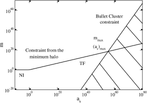
Figure 5: The initially upper curve gives the DM particle mass versus scattering length relation in order to match the characteristics of the minimum halo [see Eq. (75)]. The mass is normalized by $m_{0}$ and the scattering length by $a^{\prime}_{*}$. The initially lower curve gives the Bullet Cluster constraint from Eq. (83). Only the region above this curve is allowed by the observations. The intersection between these two curves determines the maximum DM particle mass $m_{\rm max}/m_{0}=3.79\times 10^{18}$ and its maximum scattering length $(a_{s})_{\rm max}/a^{\prime}_{*}=5.45\times 10^{55}$, leading to the results of Eq. (IV.2). We note that the intersection occurs in the TF regime where Eq. (75) can be approximated by Eq. (80).

The BECTF model discussed previously corresponds to the case where the bound fixed by the Bullet Cluster is reached. For comparison, we can consider a BECt model which corresponds to the transition between the NI limit and the TF limit. It is obtained by substituting Eq. (78) into Eq. (80), or Eq. (79) into Eq. (81), giving

$$m_{\rm t}=2.92\times 10^{-22}\,{\rm eV}/c^{2},\quad(a_{s})_{\rm t}=8.13\times 10^{-62}\,{\rm fm}$$

$$({\rm BECt})\qquad$$ (85)

This corresponds to the scales $m_{0}$ and $a^{\prime}_{*}$ defined by Eqs. (76) and (77).

IV.3 Attractive self-interaction

For bosons with an attractive self-interaction ($a_{s}<0$), the relation (75) reveals the existence of a minimum scattering length

$$\frac{(a_{s})_{\rm min}}{a^{\prime}_{*}}=-\frac{2}{3\sqrt{3}}\qquad{\rm at\quad which}\qquad\frac{m_{*}}{m_{0}}=\frac{1}{\sqrt{3}}.$$ (86)

We find $(a_{s})_{\rm min}=-1.20\times 10^{-62}\,{\rm fm}$ and $m_{*}=1.78\times 10^{-22}\,{\rm eV}/c^{2}$. The NI regime corresponds to $|a_{s}|\ll a^{\prime}_{*}$ and $m\sim m_{0}$. The NG regime corresponds to $|a_{s}|\ll a^{\prime}_{*}$ and $m\ll m_{0}$ such that

$$\frac{m}{m_{0}}\sim\frac{|a_{s}|}{a^{\prime}_{*}}.$$ (87)

In the NG regime, the mass-scattering length relation (87) can be written as

$$\frac{|a_{s}|}{m}=\frac{aR}{b^{2}M}=1.01\times 10^{-40}\,{\rm fm}/({\rm eV/c^{2}}),$$ (88)

which is equivalent to Eq. (68). It is important to note that the minimum scattering length $(a_{s})_{\rm min}$ does not correspond to the critical point (associated with the maximum mass $M_{\rm max}$) separating stable from unstable equilibrium states. This latter is located at

$$\frac{(a_{s})_{c}}{a^{\prime}_{*}}=-\frac{1}{2\sqrt{2}},\qquad\frac{m_{c}}{m_{0}}=\frac{1}{\sqrt{2}}.$$ (89)

The equilibrium states with $m<m_{c}$ are unstable (they correspond to configurations with $R<R_{*}$) so that only the equilibrium states with $m>m_{c}$ are stable (they correspond to configurations with $R>R_{*}$). Therefore, in the attractive case, the scattering length of the DM boson must lie in the range $(a_{s})_{c}<a_{s}<0$ and its mass must lie in the range $m_{c}<m<m_{0}$, with

$$m_{\rm c}=2.19\times 10^{-22}\,{\rm eV}/c^{2},\quad(a_{s})_{c}=-1.11\times 10^{-62}\,{\rm fm}$$

$$({\rm BECcrit})\qquad$$ (90)

There is no equilibrium state with $a_{s}<(a_{s})_{\rm min}$ and the equilibrium states with $(a_{s})_{\rm min}<a_{s}<(a_{s})_{c}$ are unstable. We note that, in the attractive case, the mass $m$ does not change substantially from its value $m_{0}$ in the NI limit. The BECcrit model from Eq. (90) corresponds to the case where the minimum halo is critical (i.e. its mass $M=10^{8}\,M_{\odot}$ is equal to $M_{\rm max}$).

IV.4 Constraints from particle physics and cosmology

For bosons with an attractive self-interaction, like the axion marshrevue , it is more convenient to express the results in terms of the decay constant $f$ instead of the scattering length $a_{s}$. They are related by (see, e.g., phi6 )

$$f=\left(\frac{\hbar c^{3}m}{32\pi|a_{s}|}\right)^{1/2}.$$ (91)

Particle physics and cosmology lead to the following relation between $f$ and $m$ hui :

$$\Omega_{\rm axion}\sim 0.1\left(\frac{f}{10^{17}\,{\rm GeV}}\right)^{2}\left(\frac{m}{10^{-22}\,{\rm eV}/c^{2}}\right)^{1/2},$$ (92)

where $\Omega_{\rm axion}$ is the present fraction of axions in the universe. Taking $\Omega_{\rm axion}\sim\Omega_{\rm m,0}=0.3089$ (assuming that DM is exclusively made of axions), this relation can be rewritten as

$$\frac{m^{3/2}}{|a_{s}|}=1.57\times 10^{35}\,({\rm eV/c^{2}})^{3/2}/{\rm fm}$$ (93)

or, in dimensionless form, as

$$\frac{(m/m_{0})^{3/2}}{|a_{s}|/a^{\prime}_{*}}=9.06\times 10^{5}.$$ (94)

Considering the intersection between the curves defined by Eqs. (75) and (94), we find that $m\simeq m_{0}$. Then, taking $m=m_{0}=2.92\times 10^{-22}\,{\rm eV}/c^{2}$ [see Eq. (78)] and using Eq. (93) we get $a_{s}=-3.18\times 10^{-68}\,{\rm fm}$. Therefore, we can determine $a_{s}$ and $m$ individually. We find

$$m_{\rm th}=2.92\times 10^{-22}\,{\rm eV}/c^{2},\quad(a_{s})_{\rm th}=-3.18\times 10^{-68}\,{\rm fm}$$

$$({\rm BECth})\qquad$$ (95)

We note that $m$ has approximately the same value as in the noninteracting model while $a_{s}$ has a nonzero value. It corresponds to a decay constant $f_{\rm th}=1.34\times 10^{17}\,{\rm GeV}$. Interestingly, $f$ lies in the range $10^{16}\,{\rm GeV}\leq f\leq 10^{18}\,{\rm GeV}$ expected in particle physics ($f$ is bounded above by the reduced Planck mass and below by the grand unified scale of particle physics) hui . We note that $|a_{s}|_{\rm th}\ll a^{\prime}_{*}$ so we are essentially in the NI regime. This is confirmed by the following discussion.

The maximum mass prd1 of a self-gravitating BEC made of bosons with mass $m_{\rm th}=2.92\times 10^{-22}\,{\rm eV}/c^{2}$ and scattering length $(a_{s})_{\rm th}=-3.18\times 10^{-68}\,{\rm fm}$ is $M_{\rm max}=5.10\times 10^{10}\,M_{\odot}$ and the corresponding radius is $R_{99}^{*}=1.09\,{\rm pc}$. The minimum halo ($M=10^{8}\,M_{\odot}$, $R=1\,{\rm kpc}$) has a mass much smaller than the maximum mass, so it is stable ($M<M_{\rm max}$). Larger halos have a core-halo structure with a quantum core and an approximately isothermal halo. The mass $M_{c}$ of the core increases with the halo mass $M_{h}$. Therefore, above a critical halo mass value $(M_{h})_{\rm max}$, the core mass passes above the maximum mass ($M_{c}>M_{\rm max}$) and collapses. The outcome of the collapse (dense axion star, black hole, bosenova…) is discussed in braaten ; cotner ; bectcoll ; ebycollapse ; tkachevprl ; helfer ; phi6 ; visinelli ; moss . The core mass – halo mass relation of self-interacting bosons has been determined in mcmh ; mcmhbh (without or with the presence of a central black hole). It is found that the maximum halo mass (at which $M_{c}=M_{\rm max}$) is given by mcmh

$$(M_{h})_{\rm max}=2255\frac{f^{4}}{\hbar^{2}c^{6}\Sigma_{0}},$$ (96)

where $\Sigma_{0}=141\,M_{\odot}/{\rm pc}^{2}$ is the universal surface density of DM halos kormendy ; spano ; donato . We note that the maximum halo mass $(M_{h})_{\rm max}$ depends only on $f$ while the maximum core mass $M_{\rm max}$ depends on $f$ and $m$ [see Eq. (211)]. For $f_{\rm th}=1.34\times 10^{17}\,{\rm GeV}$, we find $(M_{h})_{\rm max}=1.01\times 10^{20}\,M_{\odot}$. Since the largest DM halos observed in the Universe have a much smaller mass, $M_{h}\sim 10^{14}\,M_{\odot}\ll(M_{h})_{\rm max}$, these results suggest that the effect of an attractive self-interaction is negligible for what concerns the structure of DM halos in the nonlinear regime: Everything happens as if the bosons were not self-interacting. This conclusion assumes that Eq. (92) is fulfilled hui (see also the Remark below).

In conclusion, bosons with an attractive self-interaction are essentially equivalent to noninteracting bosons in situations of astrophysical interest while bosons with a repulsive self-interaction can be very different from noninteracting bosons (their mass $m$ may be $18$ orders of magnitude larger).

Remark: As shown above (in line with mcmh ), the quantum cores of BECDM halos with an attractive self-interaction are always stable ($M_{c}<M_{\rm max}$ of prd1 ). Because of the constraints from particle physics and cosmology hui , an attractive self-interaction is usually negligible. An attractive self-interaction would be important in sufficiently large DM halos, and lead to the collapse of the quantum core ($M_{c}>M_{\rm max}$ of prd1 ), if $f<4.22\times 10^{15}\,{\rm GeV}$ [the bound corresponds to $(M_{h})_{\rm max}=10^{14}\,M_{\odot}$ in Eq. (96)]. This is outside of the range $10^{16}\,{\rm GeV}\leq f\leq 10^{18}\,{\rm GeV}$ expected in particle physics hui [NB: if $f\sim 10^{15}\,{\rm GeV}$ is allowed then the quantum core of sufficiently large DM halos, with mass $M_{h}\gtrsim(M_{h})_{\rm max}=10^{14}\,M_{\odot}$, can collapse since $M_{c}>M_{\rm max}$]. On the other hand, it is shown in Appendix C of mcmhbh that the quantum cores of BECDM halos with a vanishing or a repulsive self-interaction are always Newtonian, i.e., their mass is always much smaller than the general relativistic maximum mass ($M_{c}\ll M_{\rm max}^{\rm GR}$ of kaup ; rb ; colpi ; chavharko ) so they cannot collapse towards a black hole. In conclusion, the cores of BECDM halos are expected to be stable in all cases of astrophysical interest. They represent large quantum bulges. They may, however, evolve collisionally on a secular timescale and ultimately collapse towards a supermassive black hole via the process of gravothermal catastrophe followed by a dynamical instability of general relativistic origin balberg if the halo mass $M_{h}$ is sufficiently large (above the microcanonical critical point), as advocated in modeldm .

IV.5 QCD axions

In the previous sections, we have determined some constraints that the mass $m$ and the scattering length $a_{s}$ of the bosons possibly composing DM must satisfy so that they are able to form giant BECs of mass $M\sim 10^{8}\,M_{\odot}$ and radius $R\sim 1\,{\rm kpc}$ comparable to dSphs like Fornax. This leads to ULAs with a very small mass that are allowed by particle physics (in connection to string theory) but that have not been fully characterized yet marshrevue . On the other hand, the characteristics of the QCD axion are precisely known from cosmology and particle physics and we can see how they enter into the problem.

QCD axions have a mass $m=10^{-4}\,{\rm eV}/c^{2}$ and a negative scattering length $a_{s}=-5.8\times 10^{-53}\,{\rm m}$ kc , corresponding to a dimensionless self-interaction constant $\lambda=-7.39\times 10^{-49}$ and a decay constant $f=5.82\times 10^{19}\,{\rm eV}$ (see Appendix C). The maximum mass of QCD axion stars is $M_{\rm max}^{\rm exact}=6.46\times 10^{-14}\,M_{\odot}$ and their minimum stable radius is $(R_{99}^{*})^{\rm exact}=227\,{\rm km}$ (their average maximum density is $\overline{\rho}=2.62\times 10^{3}\,{\rm g/m^{3}}$ and the maximum number of axions in an axion star is $N_{\rm max}=M_{\rm max}/m=7.21\times 10^{56}$).

These values of $M_{\rm max}$ and $R_{99}^{*}$ correspond to the typical size of asteroids. Obviously, QCD axions cannot form giant BECs with the dimension of DM halos like Fornax. However, they can form mini boson stars (mini axion stars or dark matter stars) of very low mass – axteroids – that could be the constituents of DM halos under the form of mini massive compact halo objects (mini MACHOs) bectcoll ; phi6 . These mini axion stars are Newtonian self-gravitating BECs of QCD axions with an attractive self-interaction stabilized by the quantum pressure (Heisenberg uncertainty principle). They may cluster into structures similar to standard CDM halos. They might play a role as DM components (i.e. DM halos could be made of mini axion stars interpreted as MACHOs instead of WIMPs) if they exist in the Universe in abundance. However, mini axion stars (MACHOs) behave essentially as CDM and do not solve the small-scale crisis of CDM.

Remark: The collapse of axion stars above the limiting mass $M_{\rm max}$ prd1 has been discussed by several authors braaten ; cotner ; bectcoll ; ebycollapse ; tkachevprl ; helfer ; phi6 ; visinelli ; moss . The collapse may lead to the formation of a dense axion star or a black hole. It may also be accompanied by an explosion with an ejection of relativistic axions (bosenova).

V Jeans mass-radius relation

In this section, we study how the Jeans length $\lambda_{J}$ and the Jeans mass $M_{J}$ of self-gravitating BECs depend on the density $\rho$. We apply these results in a cosmological context, during the matter era, where the density of BECDM evolves with time as (see, e.g., suarezchavanisprd3 for more details)

$$\frac{\rho}{\rm g/m^{3}}=2.25\times 10^{-24}\,a^{-3},$$ (97)

where $a$ is the scale factor. The beginning of the matter era, which can be identified with the epoch of radiation-matter equality (i.e. the transition between the radiation era and the matter era) occurs at $a_{\rm eq}=2.95\times 10^{-4}$. At that moment, the DM density is $\rho_{\rm eq}=8.77\times 10^{-14}\,{\rm g}/{\rm m}^{3}$. In comparison, the present density of DM is $\rho_{0}=2.25\times 10^{-24}\,{\rm g/m^{3}}$ (corresponding to $a_{0}=1$). In the following, we compute the Jeans scales $\lambda_{J}$ and $M_{J}$ for any value of the density between the epoch of radiation-matter equality $\rho_{\rm eq}$ and the present epoch $\rho_{0}$.

The Jeans instability analysis is valid during the linear regime of structure formation (it describes their initiation) which is expected to be close to the epoch of radiation-matter equality which marks the beginning of the matter era. By contrast, at the present epoch, nonlinear effects have become important (the DM halos are already formed) and the Jeans instability analysis is not valid anymore except at very large scales. We stress that the Jeans scales can only give an order of magnitude of the size and mass of the DM halos since these objects result from a very nonlinear process of free fall and violent relaxation which extends far beyond the linear regime. It is therefore not straightforward to relate quantitatively the characteristic sizes, masses and densities of DM halos to the Jeans scales. Nevertheless, the Jeans approach provides a simple first step towards the problem of structure formation.

Let us consider a standard BEC at $T=0$ with an equation of state given by Eq. (19). Using the corresponding expression of the speed of sound, the Jeans wavenumber (57) can be written as prd1

$$k_{J}^{2}=\frac{8\pi|a_{s}|\rho}{m}\left[\sqrt{1+\frac{Gm^{4}}{4\pi a_{s}^{2}\hbar^{2}\rho}}-{\rm sgn}(a_{s})\right].$$ (98)

The Jeans radius and the Jeans mass defined by Eq. (58) are then given by

$$R_{J}=\frac{\left(\frac{\pi m}{8|a_{s}|\rho}\right)^{1/2}}{\left[\sqrt{1+\frac{Gm^{4}}{4\pi a_{s}^{2}\hbar^{2}\rho}}-{\rm sgn}(a_{s})\right]^{1/2}},$$ (99)

$$M_{J}=\frac{\frac{4}{3}\pi\left(\frac{\pi m}{8|a_{s}|}\right)^{3/2}}{\rho^{1/2}\left[\sqrt{1+\frac{Gm^{4}}{4\pi a_{s}^{2}\hbar^{2}\rho}}-{\rm sgn}(a_{s})\right]^{3/2}}.$$ (100)

Eliminating the density between Eqs. (99) and (100), we obtain the Jeans mass-radius relation

$$M_{J}=\frac{\frac{\pi^{4}}{12}\frac{\hbar^{2}}{Gm^{2}R_{J}}}{1-\pi^{2}\frac{a_{s}\hbar^{2}}{Gm^{3}R_{J}^{2}}}.$$ (101)

As noted in prd1 , this expression is similar to the approximate mass-radius relation of BECDM halos given by Eq. (60). Comparing Eqs. (60) and (101), we get $a_{J}=\pi^{4}/12\simeq 8.12$ and $b_{J}=\pi$ which are close to the values of $a$ and $b$ obtained in Sec. III. This agreement is striking because the Jeans mass-radius relation [Eq. (101)] is valid in the linear regime of structure formation close to spatial homogeneity while the mass-radius relation of BECDM halos [Eq. (60)] is valid in the strongly nonlinear regime of structure formation (after free fall and violent relaxation) for very inhomogeneous objects. Before studying the relations (99)-(101) in the general case, we consider particular limits of these relations.

V.1 NI limit

In the NI limit ($a_{s}=0$), the Jeans length and the Jeans mass are given by khlopov ; bianchi ; hu ; sikivie ; prd1

$$\lambda_{J}=2\pi\left(\frac{\hbar^{2}}{16\pi G\rho m^{2}}\right)^{1/4},\quad M_{J}=\frac{1}{6}\pi\left(\frac{\pi^{3}\hbar^{2}\rho^{1/3}}{Gm^{2}}\right)^{3/4}.$$ (102)

They can be written as

$$\frac{\lambda_{J}}{\rm pc}=1.16\times 10^{-12}\,\left(\frac{{\rm eV}/c^{2}}{m}\right)^{1/2}\left(\frac{\rm g/m^{3}}{\rho}\right)^{1/4},$$ (103)

$$\frac{M_{J}}{M_{\odot}}=1.20\times 10^{-20}\,\left(\frac{{\rm eV}/c^{2}}{m}\right)^{3/2}\left(\frac{\rho}{\rm g/m^{3}}\right)^{1/4}.$$ (104)

Using Eq. (97), we find that the Jeans length increases as $a^{3/4}$ while the Jeans mass decreases as $a^{-3/4}$. Eliminating the density between the relations of Eq. (102), we obtain

$$M_{J}\lambda_{J}=\frac{\pi^{4}}{6}\frac{\hbar^{2}}{Gm^{2}}.$$ (105)

This relation is similar to the mass-radius relation (42) of Newtonian BECDM halos made of noninteracting bosons membrado ; prd1 ; prd2 .

V.2 TF limit

Let us consider bosons with a repulsive self-interaction ($a_{s}>0$). In the TF limit ($\hbar=0$), the Jeans length and the Jeans mass are given by prd1

$$\lambda_{J}=2\pi\left(\frac{a_{s}\hbar^{2}}{Gm^{3}}\right)^{1/2},\quad M_{J}=\frac{1}{6}\pi\rho\left(\frac{4\pi^{2}a_{s}\hbar^{2}}{Gm^{3}}\right)^{3/2}.$$ (106)

They can be written as

$$\frac{\lambda_{J}}{\rm pc}=34.9\,\left(\frac{a_{s}}{\rm fm}\right)^{1/2}\left(\frac{{\rm eV}/c^{2}}{m}\right)^{3/2},$$ (107)

$$\frac{M_{J}}{M_{\odot}}=3.30\times 10^{20}\,\left(\frac{a_{s}}{\rm fm}\right)^{3/2}\left(\frac{{\rm eV}/c^{2}}{m}\right)^{9/2}\frac{\rho}{\rm g/m^{3}}.$$ (108)

We note that the Jeans length is independent of the density prd1 . Using Eq. (97), we find that the Jeans mass decreases as $a^{-3}$. The relation from Eq. (106) is similar to the relation (45) determining the radius of a self-interacting BECDM halo in the TF approximation tkachev ; maps ; leekoh ; goodman ; arbey ; bohmer ; prd1 .

V.3 NG limit

Let us consider bosons with an attractive self-interaction ($a_{s}<0$). In the nongravitational limit ($G=0$), the Jeans length and the Jeans mass are given by prd1

$$\lambda_{J}=2\pi\left(\frac{m}{16\pi|a_{s}|\rho}\right)^{1/2},\quad M_{J}=\frac{\pi}{6}\frac{1}{\rho^{1/2}}\left(\frac{\pi m}{4|a_{s}|}\right)^{3/2}.$$ (109)

They can be written as

$$\frac{\lambda_{J}}{\rm pc}=3.83\times 10^{-26}\,\left(\frac{\rm fm}{|a_{s}|}\right)^{1/2}\left(\frac{m}{{\rm eV}/c^{2}}\right)^{1/2}\left(\frac{\rm g/m^{3}}{\rho}\right)^{1/2},$$ (110)

$$\frac{M_{J}}{M_{\odot}}=4.36\times 10^{-61}\,\left(\frac{\rm fm}{|a_{s}|}\right)^{3/2}\left(\frac{m}{{\rm eV}/c^{2}}\right)^{3/2}\left(\frac{\rm g/m^{3}}{\rho}\right)^{1/2}.$$ (111)

Using Eq. (97), we find that the Jeans length and the Jeans mass both increase as $a^{3/2}$. Eliminating the density between the relations of Eq. (109), we obtain

$$M_{J}=\frac{\pi^{2}}{24}\frac{m}{|a_{s}|}\lambda_{J}.$$ (112)

This relation is similar to the mass-radius relation of nongravitational BECDM halos with an attractive self-interaction given by Eq. (49) prd2 . We recall, however, that these equilibrium states (valid in the nonlinear regime of structure formation) are unstable so they should not be observed in practice (see prd1 for detail). Therefore, only the relations (109)-(112) obtained from the Jeans analysis in the linear regime of structure formation are physically meaningful. They determine the initiation of structures (clumps) in a homogeneous BEC due to the attractive self-interaction of the bosons. Their evolution in the nonlinear regime requires a specific analysis. Since these clumps cannot evolve towards stable DM halos with mass $M\sim M_{J}$ and radius $R\sim R_{J}$, they are expected to collapse towards smaller structures until repulsive terms in the self-interaction potential (not considered here) come into play phi6 .

V.4 Repulsive self-interaction

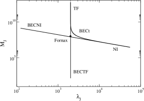
Figure 7: Jeans-mass radius relation for bosons with a repulsive self-interaction for the three models BECNI, BECTF and BECt described in the text. We see that the Jeans mass-radius relation (linear regime) is similar to the mass-radius relation of DM halos (nonlinear regime) represented in Fig. 2.

In order to determine the evolution of the Jeans scales with the density, we need to specify the parameters of the DM particle. For illustration, we use the parameters obtained in Sec. IV (see also Appendix D of abrilphas and Sec. II of mcmh ). They have been obtained in order to match the characteristics of a “minimum halo” of radius $R\sim 1\,{\rm kpc}$ and mass $M\sim 10^{8}\,M_{\odot}$, similar to Fornax, interpreted as the ground state of the self-gravitating BEC. We use this procedure to determine the parameters of the DM particle, then compute the Jeans scales at the epoch of radiation-matter equality and at the present epoch, instead of trying to determine the parameters of the DM particle directly from the Jeans scales. In the present section, we consider the case of bosons with a repulsive self-interaction (or no self-interaction). We consider different types of DM particles denoted BECNI, BECTF and BECt in Sec. IV. For each of these particles, the evolution of the Jeans length $\lambda_{J}$ and Jeans mass $M_{J}$ as a function of the inverse density $1/\rho$ (which increases with time as the Universe expands) is plotted in Fig. 6. The Jeans mass-radius relation (parameterized by the density) is plotted in Fig. 7. The curves start from the epoch of matter-radiation equality and end at the present epoch.

Generically, as the density of the universe decreases, the BEC is first in the TF regime then in the NI regime. In the TF regime the Jeans length is constant while the Jeans mass decreases like $\rho$ (see Sec. V.2). In the NI regime the Jeans length increases like $\rho^{-1/4}$ while the Jeans mass decreases like $\rho^{1/4}$ (see Sec. V.1). The transition between the TF regime and the NI regime occurs at a typical density

$$\rho_{s}=\frac{Gm^{4}}{16\pi\hbar^{2}a_{s}^{2}}$$ (113)

obtained by equating Eqs. (102) and (106). At that point

$$(M_{J})_{s}=\frac{\pi^{3}}{12}\frac{\hbar}{\sqrt{Gma_{s}}}$$ (114)

and

$$(\lambda_{J})_{s}=2\pi\left(\frac{a_{s}\hbar^{2}}{Gm^{3}}\right)^{1/2}.$$ (115)

The BEC is always in the NI regime (during the period going from the epoch of matter-radiation equality to the present epoch) if $1/\rho_{s}<1/\rho_{\rm eq}$, i.e., if

$$\frac{a_{s}}{m^{2}}<\left(\frac{G}{16\pi\hbar^{2}\rho_{\rm eq}}\right)^{1/2}=3.71\times 10^{-21}\,\frac{\rm fm}{({\rm eV}/c^{2})^{2}}.$$ (116)

Combining this inequality with the $m(a_{s})$ relation of Sec. IV, we find that the BEC is always in the NI regime if $0\leq a_{s}\leq 3.16\times 10^{-64}\,{\rm fm}$ (and $m\sim 2.92\times 10^{-22}\,{\rm eV}/c^{2}$). This corresponds to $0\leq\lambda\leq 1.17\times 10^{-92}$. On the other hand, the BEC is always in the TF regime (during the same period) if $1/\rho_{s}>1/\rho_{0}$, i.e., if

$$\frac{a_{s}}{m^{2}}>\left(\frac{G}{16\pi\hbar^{2}\rho_{0}}\right)^{1/2}=7.32\times 10^{-16}\,\frac{\rm fm}{({\rm eV}/c^{2})^{2}}.$$ (117)

Combining this inequality with the $m(a_{s})$ relation of Sec. IV, we find that the BEC is always in the TF regime if $3.65\times 10^{-53}\,{\rm fm}\leq a_{s}\leq(a_{s})_{\rm max}=4.41\times 10^{-6}\,{\rm fm}$ (and $2.23\times 10^{-19}\,{\rm eV}/c^{2}\leq m\leq m_{\rm max}=1.10\times 10^{-3}\,{\rm eV}/c^{2}$). This corresponds to $1.04\times 10^{-78}\leq\lambda\leq\lambda_{\rm max}=6.18\times 10^{-16}$.

BECNI: Let us consider noninteracting ULAs with a mass $m=2.92\times 10^{-22}\,{\rm eV}/c^{2}$ determined by the characteristics of the minimum halo (see Sec. IV). At the epoch of radiation-matter equality, we find $\lambda_{J}=124\,{\rm pc}$ and $M_{J}=1.31\times 10^{9}\,M_{\odot}$ (the comoving Jeans length is $\lambda_{J}^{c}=\lambda_{J}/a=0.420\,{\rm Mpc}$). At the present epoch, we find $\lambda_{J}=55.3\,{\rm kpc}$ and $M_{J}=2.94\times 10^{6}\,M_{\odot}$.

BECTF: Let us consider self-interacting bosons with a mass $m=1.10\times 10^{-3}\,{\rm eV}/c^{2}$ and a scattering length $a_{s}=4.41\times 10^{-6}\,{\rm fm}$ (this yields $\lambda=6.18\times 10^{-16}$). This corresponds to a ratio $a_{s}/m^{3}=3.28\times 10^{3}\,{\rm fm}/({\rm eV/c^{2}})^{3}$ determined by the radius of the minimum halo and to a ratio $4\pi a_{s}^{2}/m=1.25\,{\rm cm^{2}/g}$ determined by the constraint set by the Bullet Cluster assuming that the bound is reached (see Sec. IV). For the period considered, the BEC is always in the TF regime. At the epoch of radiation-matter equality, we find $\lambda_{J}=2.01\,{\rm kpc}$ and $M_{J}=5.51\times 10^{12}\,M_{\odot}$ (the comoving Jeans length is $\lambda_{J}^{c}=\lambda_{J}/a=6.81\,{\rm Mpc}$). At the present epoch we find $\lambda_{J}=2.01\,{\rm kpc}$ and $M_{J}=141\,M_{\odot}$.

BECt: Let us consider self-interacting bosons with a mass $m=2.92\times 10^{-22}\,{\rm eV}/c^{2}$ and a scattering length $a_{s}=8.13\times 10^{-62}\,{\rm fm}$ (this yields $\lambda=3.02\times 10^{-90}$). This corresponds to a ratio $a_{s}/m^{3}=3.28\times 10^{3}\,{\rm fm}/({\rm eV/c^{2}})^{3}$ determined by the radius of the minimum halo and to a scattering length chosen such that the minimum halo is just at the transition between the TF regime and the NI regime (see Sec. IV). For the period considered, the BEC is first in the TF regime then in the NI regime (the transition occurs at a typical density $\rho_{s}=1.33\times 10^{-18}\,{\rm g/m^{3}}$). At the epoch of radiation-matter equality, we find $\lambda_{J}=2.00\,{\rm kpc}$ and $M_{J}=5.39\times 10^{12}\,M_{\odot}$ (the comoving Jeans length is $\lambda_{J}^{c}=\lambda_{J}/a=6.78\,{\rm Mpc}$). At the present epoch we find $\lambda_{J}=55.3\,{\rm kpc}$ and $M_{J}=2.94\times 10^{6}\,M_{\odot}$. In the TF regime, the BECt model behaves as the BECTF model (because they have the same ratio $a_{s}/m^{3}$) and in the NI regime, the BECt model behaves as the BECNI model corresponding to noninteracting ULAs (because they have the same mass $m$).

(iv) BECf: Let us consider self-interacting bosons with a mass $m=3\times 10^{-21}\,{\rm eV}/c^{2}$ and a scattering length $a_{s}=1.11\times 10^{-58}\,{\rm fm}$ (this yields $\lambda=4.24\times 10^{-86}$). This fiducial model is motivated by cosmological considerations shapiro . It is similar to the BECt model. For the period considered, the BEC is first in the TF regime then in the NI regime (the transition occurs at a typical density $\rho_{s}=7.93\times 10^{-21}\,{\rm g/m^{3}}$). At the epoch of radiation-matter equality, we find $\lambda_{J}=2.24\,{\rm kpc}$ and $M_{J}=7.61\times 10^{12}\,M_{\odot}$ (the comoving Jeans length is $\lambda_{J}^{c}=\lambda_{J}/a=7.59\,{\rm Mpc}$). At the present epoch we find $\lambda_{J}=17.3\,{\rm kpc}$ and $M_{J}=9.05\times 10^{4}\,M_{\odot}$.

Remark: ULA clumps formed in the linear regime by Jeans instability may evolve, in the nonlinear regime, into stable DM halos with mass $M\sim M_{J}$ and radius $R\sim R_{J}$ (since self-gravitating BECs with a repulsive self-interaction are stable). They can then increase their mass by mergings and accretion (or possibly loose mass) leading to the DM halos observed in the universe. Large DM halos have a core-halo structure resulting from violent relaxation and gravitational cooling. The core mass – halo mass of self-interacting BECs has been determined in mcmh ; mcmhbh .

V.5 Attractive self-interaction

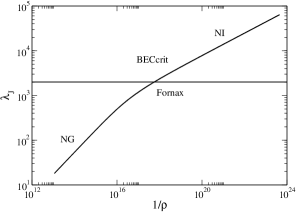
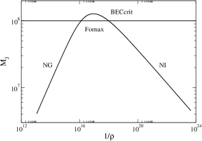
Figure 8: Evolution of the Jeans length and Jeans mass with the inverse density of the universe for bosons with an attractive self-interaction ($\lambda_{J}$ is in ${\rm pc}$, $M_{J}$ is in solar masses $M_{\odot}$, and $\rho$ is in ${\rm g/m^{3}}$) for the BECcrit model described in the text.

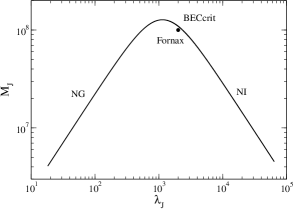
Figure 9: Jeans-mass radius relation for bosons with an attractive self-interaction for the BECcrit model described in the text. We note that the Jeans mass-radius relation (linear regime) is similar to the mass-radius relation of DM halos (nonlinear regime) represented in Fig. 3.

In this section, we consider the case of bosons with an attractive self-interaction. We consider different types of DM particles denoted BECcrit, BECth and QCD axions in Sec. IV. For each of these particles, the evolution of the Jeans length $\lambda_{J}$ and Jeans mass $M_{J}$ as a function of the inverse density $1/\rho$ (which increases with time as the universe expands) is plotted in Fig. 8. The Jeans mass-radius relation (parameterized by the density) is plotted in Fig. 9. The curves start from the epoch of matter-radiation equality and end at the present epoch.

Generically, as the density of the universe decreases, the BEC is first in the NG regime then in the NI regime. In the NG regime the Jeans length and the Jeans mass both increase like $\rho^{-1/2}$ (see Sec. V.3). In the NI regime the Jeans length increases like $\rho^{-1/4}$ while the Jeans mass decreases like $\rho^{1/4}$ (see Sec. V.1). There is a maximum Jeans mass

$$(M_{J})_{\rm max}=\frac{\pi^{3}}{24}\frac{\hbar}{\sqrt{Gm|a_{s}|}},$$ (118)

corresponding to a Jeans length

$$(\lambda_{J})_{*}=2\pi\left(\frac{|a_{s}|\hbar^{2}}{Gm^{3}}\right)^{1/2},$$ (119)

at the density

$$\rho_{*}=\frac{Gm^{4}}{32\pi\hbar^{2}a_{s}^{2}}.$$ (120)

The transition between the NG regime and the NI regime occurs at a typical density

$$\rho_{s}=\frac{Gm^{4}}{16\pi\hbar^{2}a_{s}^{2}},$$ (121)

obtained by equating Eqs. (102) and (109). At that point

$$(M_{J})_{s}=\frac{\pi^{3}}{12}\frac{\hbar}{\sqrt{Gm|a_{s}|}}$$ (122)

and

$$(\lambda_{J})_{s}=2\pi\left(\frac{|a_{s}|\hbar^{2}}{Gm^{3}}\right)^{1/2}.$$ (123)

These scales are similar to those corresponding to the maximum mass (we have $\rho_{s}=2\rho_{*}$, $(M_{J})_{s}=2(M_{J})_{\rm max}$ and $(\lambda_{J})_{s}=(\lambda_{J})_{*}$). The BEC is always in the NI regime (during the period going from the epoch of matter-radiation equality to the present epoch) if $1/\rho_{s}<1/\rho_{\rm eq}$, i.e., if

$$\frac{|a_{s}|}{m^{2}}<\left(\frac{G}{16\pi\hbar^{2}\rho_{\rm eq}}\right)^{1/2}=3.71\times 10^{-21}\,\frac{\rm fm}{({\rm eV}/c^{2})^{2}}.$$ (124)

Combining this inequality with the $m(a_{s})$ relation of Sec. IV, we find that the BEC is always in the NI regime if $-3.16\times 10^{-64}\,{\rm fm}\leq a_{s}\leq 0$ and $m\sim 2.92\times 10^{-22}\,{\rm eV}/c^{2}$. This corresponds to $-1.18\times 10^{-92}\leq\lambda\leq 0$ and $f\geq 1.35\times 10^{15}\,{\rm GeV}$. On the other hand, the BEC is always in the NG regime (during the same period) if $1/\rho_{s}>1/\rho_{0}$, i.e., if

$$\frac{|a_{s}|}{m^{2}}>\left(\frac{G}{16\pi\hbar^{2}\rho_{0}}\right)^{1/2}=7.32\times 10^{-16}\,\frac{\rm fm}{({\rm eV}/c^{2})^{2}}.$$ (125)

Combining this inequality with the $m(a_{s})$ relation of Sec. IV, we find that the BEC is always in the NG regime if $-1.39\times 10^{-65}\,{\rm fm}\leq a_{s}\leq 0$ and $m\leq 1.38\times 10^{-25}\,{\rm eV/c^{2}}$. This corresponds to $-2.44\times 10^{-97}\leq\lambda\leq 0$ and $f\sim f_{\rm min}=1.39\times 10^{14}\,{\rm GeV}$.

BECcrit: Let us consider self-interacting bosons with a mass $m=2.19\times 10^{-22}\,{\rm eV}/c^{2}$ and a scattering length $a_{s}=-1.11\times 10^{-62}\,{\rm fm}$ (this yields $\lambda=-3.10\times 10^{-91}$ and $f=1.97\times 10^{14}\,{\rm GeV}$). These values are obtained by requiring that the minimum halo is critical (see Sec. IV). For the period considered, the BEC is first in the NG regime then in the NI regime (the transition occurs at a typical density $\rho_{s}=2.25\times 10^{-17}\,{\rm g/m^{3}}$). The Jeans mass is maximal at the density $\rho_{*}=1.13\times 10^{-17}\,{\rm g/m^{3}}$. At that density $(M_{J})_{\rm max}=1.27\times 10^{8}\,M_{\odot}$ and $(\lambda_{J})_{*}=1.13\,{\rm kpc}$. At the epoch of radiation-matter equality, we find $\lambda_{J}=18.2\,{\rm pc}$ and $M_{J}=4.08\times 10^{6}\,M_{\odot}$ (the comoving Jeans length is $\lambda_{J}^{c}=\lambda_{J}/a=0.0617\,{\rm Mpc}$). At the present epoch, we find $\lambda_{J}=63.8\,{\rm kpc}$ and $M_{J}=4.53\times 10^{6}\,M_{\odot}$.

BECth: Let us consider self-interacting bosons with a mass $m=2.92\times 10^{-22}\,{\rm eV}/c^{2}$ and a scattering length $a_{s}=-3.18\times 10^{-68}\,{\rm fm}$ (this yields $\lambda=-1.18\times 10^{-96}$ and $f=1.34\times 10^{17}\,{\rm GeV}$). These values are obtained by using constraints from particle physics and cosmology (see Sec. IV.4). For the period considered, the BEC is always in the NI regime (see the BECNI case studied above). At the epoch of radiation-matter equality, we find $\lambda_{J}=124\,{\rm pc}$ and $M_{J}=1.31\times 10^{9}\,M_{\odot}$ (the comoving Jeans length is $\lambda_{J}^{c}=\lambda_{J}/a=0.420\,{\rm Mpc}$). At the present epoch, we find $\lambda_{J}=55.3\,{\rm kpc}$ and $M_{J}=2.94\times 10^{6}\,M_{\odot}$. The Jeans mass is always much below the maximum Jeans mass $(M_{J})_{\rm max}=6.52\times 10^{10}\,M_{\odot}$ reached at a density $\rho_{*}=4.33\times 10^{-6}\,{\rm g/m^{3}}$. These results show that the effect of an attractive self-interaction is negligible for what concerns the formation of structures in the linear regime: Everything happens as if the bosons were not self-interacting.

QCD axions: Let us consider QCD axions with a mass $m=10^{-4}\,{\rm eV}/c^{2}$ and a scattering length $a_{s}=-5.8\times 10^{-53}\,{\rm m}$ (this yields $\lambda=-7.39\times 10^{-49}$ and $f=5.82\times 10^{10}\,{\rm GeV}$). For the period considered (matter era), the axions are always in the NI regime. At the epoch of radiation-matter equality, we find $\lambda_{J}=2.13\times 10^{-7}\,{\rm pc}$ and $M_{J}=6.52\times 10^{-18}\,M_{\odot}$ (the comoving Jeans length is $\lambda_{J}^{c}=\lambda_{J}/a=7.22\times 10^{-10}\,{\rm Mpc}$). At the present epoch we find $\lambda_{J}=9.45\times 10^{-5}\,{\rm pc}$ and $M_{J}=1.47\times 10^{-20}\,M_{\odot}$. The Jeans mass is always much below the maximum Jeans mass $(M_{J})_{\rm max}=8.25\times 10^{-14}\,M_{\odot}$ reached at a density $\rho_{*}=1.79\times 10^{4}\,{\rm g/m^{3}}$. These results show that the effect of an attractive self-interaction is negligible for what concerns the formation of structures in the linear regime: Everything happens as if the QCD axions were not self-interacting. Furthermore, the Jeans scales computed above are much smaller than the galactic scales indicating the QCD axions essentially behave as CDM.

Remark: QCD axions clumps formed in the linear regime by Jeans instability may evolve, in the nonlinear regime, into stable dilute axion stars (since noninteracting self-gravitating BECs are stable). They can then increase their mass by mergings and accretion (or possibly loose mass). If their mass passes above the maximum mass $M_{\rm max}=6.46\times 10^{-14}\,M_{\odot}$ they undergo gravitational collapse, leading to a bosenova or a dense axion star (see Sec. IV.5). Clumps of DM particles corresponding to the BECcrit parameters formed in the linear regime by Jeans instability cannot evolve, in the nonlinear regime, into stable configurations since nongravitational BECs are unstable (see Sec. V.3). Therefore, they are expected to directly collapse, leading to bosenovae or dense axion stars. Clumps of DM particles corresponding to the BECth parameters formed in the linear regime by Jeans instability may evolve, in the nonlinear regime, into stable DM halos with a core-halo profile (since noninteracting self-gravitating BECs are stable). They can then increase their mass by mergings and accretion. We have seen in Sec. IV.4 that, for realistic DM halos, the core mass is always smaller than the critical mass so the quantum core is always stable.

V.6 An optimal cosmological density

Except for QCD axions, all the models that we have considered above are based on values of $m$ and $a_{s}$ that are consistent with the properties of the minimum halo (see Sec. IV). Therefore, by construction, we have $M_{J}\sim 10^{8}\,M_{\odot}$ and $R_{J}\sim 1\,{\rm kpc}$ at a particular density $\rho=3M/4\pi R^{3}=1.62\times 10^{-18}\,{\rm g/m^{3}}$ in the evolution of the universe. This “optimal” density corresponds to a scale factor $a=0.0111$ and a redshift $z=1/a-1=88.6$. If the structures formed at this epoch they would have a Jeans mass and a Jeans radius comparable to the mass and size of the minimum halo ($M\sim 10^{8}\,M_{\odot}$ and $R\sim 1\,{\rm kpc}$). Actually, structures may form at a different epoch and evolve by accreting or loosing mass during the nonlinear regime. The relation between the Jeans scales (in the linear regime) and the actual scales of DM halos (in the nonlinear regime) is not straightforward and usually requires to study the nonlinear process of structure formation numerically.

VI Conclusion

In this paper, following previous works on the subject, we have considered the possibility that DM is made of bosons in the form of self-gravitating BECs. This model is interesting because it may solve the small-scale problems of the standard CDM model such as the core-cusp problem and the missing satellite problem. Indeed, in the linear regime of structure formation due to the Jeans instability, quantum mechanics (Heisenberg uncertainty principle) or a repulsive self-interaction ($a_{s}>0$) leads to a finite Jeans length $\lambda_{J}$ even at $T=0$. Therefore, gravitational collapse can take place only above a sufficiently large size and a sufficiently large mass (i.e. above $\lambda_{J}$ and $M_{J}$). The existence of a minimum size and a minimum mass is in agreement with the observations. By contrast, in the classical pressureless CDM model ($\hbar=P=0$), the Jeans length and the Jeans mass vanish ($\lambda_{J}=M_{J}=0$), or are very small, implying the possibility of formation of structures at all scales in contradiction with the observations. On the other hand, in the nonlinear regime of structure formation (after the system has experienced free fall, violent relaxation, gravitational cooling, and virialization), the BECDM model leads to DM halos with a core, i.e., the central density is finite instead of diverging as $r^{-1}$ like in the CDM model. The prediction of DM halos with a core rather than a cusp is again in agreement with the observations.

According to the above results, the BECDM model predicts the existence of a “minimum DM halo” which corresponds to the ground state of the self-gravitating BEC at $T=0$. We have identified this minimum (ultracompact) halo with dSphs like Fornax with a typical radius $R_{\rm min}=1\,{\rm kpc}$ and a typical mass $M_{\rm min}=10^{8}\,M_{\odot}$. The ground state of the self-gravitating BEC also describes the quantum core of larger halos with $M>M_{\rm min}$. This quantum core is surrounded by an approximately isothermal atmosphere (mimicking the NFW profile) yielding flat rotation curves at large distances as discussed in, e.g., modeldm .

We have first determined an accurate expression of the mass-radius relation $M(R)$ of self-gravitating BECs by combining approximate analytical results obtained from the Gaussian ansatz prd1 with exact asymptotic results obtained by solving the GPP equations numerically prd2 . Assuming that this mass-radius relation describes the minimum DM halo with $R_{\rm min}=1\,{\rm kpc}$ and $M_{\rm min}=10^{8}\,M_{\odot}$ (as well as the cores of larger DM halos) we have obtained an accurate expression of the DM mass-scattering length relation $m(a_{s})$. This relation determines the mass $m$ that the DM particle with a scattering length $a_{s}$ should have in order to yield results that are consistent with the mass and the size of the minimum halo typically representing a dSph.

For noninteracting bosons, we found

$$m=2.92\times 10^{-22}\,{\rm eV}/c^{2},$$ (126)

which is the typical mass of the DM particle considered in FDM scenarios.

For bosons with an attractive self-interaction, we found that the mass of the DM particle is restricted by the inequality

$$2.19\times 10^{-22}\,{\rm eV}/c^{2}<m<2.92\times 10^{-22}\,{\rm eV}/c^{2},$$ (127)

otherwise dSphs like Fornax would be unstable (their mass would be above the maximum mass $M_{\rm max}$ found in prd1 ). Therefore, an attractive self-interaction almost does not change the typical mass of the DM particle required to match the characteristics of the minimum halo (the boson mass is just a little smaller than the value from Eq. (126) in the noninteracting model). In addition, in line with our previous works suarezchavanisprd3 ; mcmh ; mcmhbh , we have shown that, in situations of astrophysical interest, the effect of an attractive self-interaction is negligible both in the linear (see Sec. V.5) and nonlinear (see Sec. IV.4) regimes of structure formation. Therefore, in practice, bosons with an attractive self-interaction can be considered as noninteracting.

For bosons with a repulsive self-interaction, we found that the mass of the DM particle is restricted by the inequality

$$2.92\times 10^{-22}\,{\rm eV}/c^{2}<m<1.10\times 10^{-3}\,{\rm eV}/c^{2},$$ (128)

where the maximum bound arises from the Bullet Cluster constraint. Therefore, a repulsive self-interaction can increase the typical mass of the DM particle by $18$ orders of magnitude with respect to its value in the noninteracting case. As noted in Appendix D.4 of abrilphas , a mass larger than $2.92\times 10^{-22}\,{\rm eV/c^{2}}$ could alleviate some tensions with the observations of the Lyman-$\alpha$ forest encountered in the noninteracting model. We have considered two typical models corresponding to $m=1.10\times 10^{-3}\,{\rm eV}/c^{2}$ and $a_{s}=4.41\times 10^{-6}\,{\rm fm}$ (BECTF) and $m=2.92\times 10^{-22}\,{\rm eV}/c^{2}$ and $a_{s}=8.13\times 10^{-62}\,{\rm fm}$ (BECt).

We have then shown that the Jeans mass-radius relation $M_{J}(R_{J})$, which is valid in the linear regime of structure formation, is similar to the mass-radius relation $M(R)$ of the minimum BECDM halo (or the core of large halos), corresponding to the ground state of the GPP equations, which is valid in the nonlinear regime of structure formation. This analogy allows us to directly apply some results obtained in the context of (nonlinear) self-gravitating BECs to the Jeans (linear) instability problem and vice versa.

The two curves $M_{J}(R_{J})$ and $M(R)$ are parameterized by a typical density (the density of the universe for the $M_{J}(R_{J})$ relation and the average – or central – density of the BEC for the $M(R)$ relation) going from high values to low values. For noninteracting bosons, the mass decreases as the radius increases. For bosons with a repulsive self-interaction, there is a minimum radius at which $M\rightarrow+\infty$ corresponding to the TF limit. The mass decreases as the radius increases, going from the TF limit (high densities) to the NI limit (low densities). For bosons with an attractive self-interaction, the mass first increases as the radius increases, reaches a maximum value $M_{\rm max}$, and then decreases, going from the NG limit (high densities) to the NI limit (low densities).

Despite these analogies, the curves $M_{J}(R_{J})$ and $M(R)$ have a very different physical interpretation. The curve $M_{J}(R_{J})$ determines the Jeans mass and the Jeans radius at different epochs in the history of the universe characterized by its density $\rho$ (in that case it is more relevant to plot $M_{J}(\rho)$ and $R_{J}(\rho)$ individually). The Jeans scales determine the minimum mass and the minimum size of a condensation that can become unstable and form a clump. We must be careful, however, that the Jeans instability study is valid only in the linear regime of structure formation. As a result, the interpretation of the curve $M_{J}(R_{J})$ and its domain of validity is not straightforward. In principle, the results of the linear Jeans instability study are valid only in a sufficiently young universe (typically the beginning of the matter era) where $\rho_{\rm eq}=8.77\times 10^{-14}\,{\rm g}/{\rm m}^{3}$. It is not clear if we can apply the results of the Jeans instability study at later epochs. On the other hand, the curve $M(R)$ determines the mass-radius relation of DM halos that are formed in the nonlinear regime of structure formation after having experienced free fall, violent relaxation, gravitational cooling, and virialization. It applies to the minimum halo or to the quantum core of larger halos. We expect that the mass and the size of the minimum halo is of the order of the Jeans mass and Jeans radius ($M\sim M_{J}$ and $R\sim R_{J}$) calculated at the “relevant” epoch of structure formation. There is, however, an uncertainty about what this epoch is (see Sec. V.6). Furthermore, the relation between the Jeans scales and the characteristics of DM halos is not straightforward. In practice, the linear Jeans instability occurs at a certain epoch, leading to weakly inhomogeneous clumps of mass $M_{J}$ and radius $R_{J}$. Then, these clumps evolve in the nonlinear regime ultimately leading to DM halos of minimum mass $M\sim M_{J}$ and minimum radius $R\sim R_{J}$. The DM halos may also merge (or inversely loose mass) so that their actual mass $M$ and radius $R$ may be different from $M_{J}$ and $R_{J}$. On the other hand, the $M(R)$ relation may present regions of instability such as the NG branch of Fig. 3. The solutions on these branches cannot correspond to observable DM halos since they are unstable. These branches are therefore forbidden in the nonlinear problem of structure formation. However, the corresponding branches in the Jeans mass-radius relation $M_{J}(R_{J})$ have their usual interpretation. They determine the mass and size triggering the gravitational instability in the linear regime. The existence of stable or unstable branches in the mass-radius relation $M(R)$ of DM halos leads to the different possibilities described at the end of Secs. V.4 and V.5. Typically, we have two possibilities:

(i) Consider first a branch of the $M_{J}(R_{J})$ relation such that the corresponding branch of the $M(R)$ relation is stable (for example the NI branch or the TF branch). In that case, clumps of mass $M_{J}$ and $R_{J}$ formed in the linear regime by Jeans instability evolve, in the nonlinear regime, into stable DM halos of mass $M\sim M_{J}$ and radius $R\sim R_{J}$. They can then increase their mass by mergings and accretion (or possibly loose mass) leading to the DM halos observed in the universe.

(ii) Consider now a branch of the $M_{J}(R_{J})$ relation such that the corresponding branch of the $M(R)$ relation is unstable (for example the NG branch). In that case, clumps of mass $M_{J}$ and $R_{J}$ formed in the linear regime by Jeans instability cannot evolve, in the nonlinear regime, into DM halos of mass $M\sim M_{J}$ and radius $R\sim R_{J}$ (such halos are unstable). They rather undergo an explosion tkachevprl or a violent (nonlinear) gravitational collapse leading presumably to smaller objects determined by higher order repulsive terms in the self-interaction potential braaten ; ebycollapse ; phi6 .

In the present paper, we have illustrated our results for bosons interacting via a $\phi^{4}$ potential. We have considered the case of a vanishing ($a_{s}=0$), repulsive ($a_{s}>0$) or attractive ($a_{s}<0$) self-interaction. The model of noninteracting bosons (FDM) leads to a boson mass $m\sim 10^{-22}\,{\rm eV/c^{2}}$ that creates some tensions with the observations of the Lyman-$\alpha$ forest hui . These observations require a larger mass of at least one order of magnitude. We have shown that the model of bosons with an attractive self-interaction necessitates a mass even smaller than $m\sim 10^{-22}\,{\rm eV/c^{2}}$ (according to Fig. 4 the mass $m$ decreases as $|a_{s}|$ increases when $a_{s}<0$). This model is therefore also in tension with the observations. By contrast, the model of bosons with a repulsive self-interaction allows a boson mass which can be up to $18$ orders of magnitude larger than $m\sim 10^{-22}\,{\rm eV/c^{2}}$ (according to Fig. 4 the mass $m$ increases as $a_{s}$ increases when $a_{s}>0$). As noted in abrilphas this model could alleviate some tensions with the observations of the Lyman-$\alpha$ forest encountered in the noninteracting model. As a result, a repulsive self-interaction ($a_{s}>0$) is priviledged over an attractive self-interaction ($a_{s}<0$) modeldm . A repulsive self-interaction is also favored by cosmological constraints shapiro ; abrilphas which yield a fiducial model with a mass $m=3\times 10^{-21}\,{\rm eV}/c^{2}$ and a scattering length $a_{s}=1.11\times 10^{-58}\,{\rm fm}$ (BECf). We recall that theoretical models of particle physics usually lead to particles with an attractive self-interaction (e.g., the QCD axion). However, some authors fan ; reig have pointed out the possible existence of particles with a repulsive self-interaction (e.g., the light majoron).

Appendix A Derivation of Schrödinger’s equation

In this Appendix, we briefly recall the derivation of the Schrödinger equation from the formalism of scale relativity nottale . We follow the presentation given in Ref. epjpnottale .

Nottale nottale has shown that the Schrödinger equation is equivalent to the fundamental equation of dynamics

$$\frac{D{\bf U}}{Dt}=-\nabla\Phi,$$ (129)

where ${\bf F}=-\nabla\Phi$ is the force by unit of mass exerted on a particle, provided that ${\bf U}({\bf r},t)$ is interpreted as a complex velocity field and $D/Dt$ as a complex time derivative operator (or covariant derivative) defined by

$$\frac{D}{Dt}=\frac{\partial}{\partial t}+{\bf U}\cdot\nabla-i{\cal D}\Delta,$$ (130)

where

$${\cal D}=\frac{\hbar}{2m}$$ (131)

is the Nelson nelson diffusion coefficient of quantum mechanics or the fractal fluctuation parameter in the theory of scale relativity nottale . Using the expression (130) of the covariant derivative, Eq. (129) can be rewritten as a complex viscous Burgers equation

$$\frac{\partial{\bf U}}{\partial t}+({\bf U}\cdot\nabla){\bf U}=i{\cal D}\Delta{\bf U}-\nabla\Phi$$ (132)

with an imaginary viscosity $\nu=i{\cal D}$. It can be shown nottale that the complex velocity field can be written as the gradient of a complex action:

$${\bf U}=\frac{\nabla{\cal S}}{m}.$$ (133)

This defines a potential flow. As a consequence, the flow is irrotational: $\nabla\times{\bf U}={\bf 0}$. Using the well-known identities of fluid mechanics $({\bf U}\cdot\nabla){\bf U}=\nabla({{\bf U}^{2}}/{2})-{\bf U}\times(\nabla\times{\bf U})$ and $\Delta{\bf U}=\nabla(\nabla\cdot{\bf U})-\nabla\times(\nabla\times{\bf U})$ which reduce to $({\bf U}\cdot\nabla){\bf U}=\nabla({{\bf U}^{2}}/{2})$ and $\Delta{\bf U}=\nabla(\nabla\cdot{\bf U})$ for an irrotational flow, and using the identity $\nabla\cdot{\bf U}=\Delta{\cal S}/m$ resulting from Eq. (133), we find that Eq. (132) is equivalent to the complex quantum Hamilton-Jacobi (or Bernoulli) equation

$$\frac{\partial{\cal S}}{\partial t}+\frac{1}{2m}(\nabla{\cal S})^{2}-i{\cal D}\Delta{\cal S}+m\Phi=0.$$ (134)

We now define the wave function $\psi({\bf r},t)$ through the complex Cole-Hopf transformation

$${\cal S}=-2im{\cal D}\ln\psi,$$ (135)

which is equivalently to the WKB formula

$$\psi=e^{i{\cal S}/\hbar}.$$ (136)

Substituting Eq. (135) into Eq. (134), and using the identity

$$\Delta(\ln\psi)=\frac{\Delta\psi}{\psi}-\frac{1}{\psi^{2}}(\nabla\psi)^{2},$$ (137)

we obtain the Schrödinger equation

$$i\hbar\frac{\partial\psi}{\partial t}=-\frac{\hbar^{2}}{2m}\Delta\psi+m\Phi\psi.$$ (138)

Appendix B Equivalence between the stability criteria based on the equation of pulsation and on the energy principle

B.1 Energy principle

The GPP equations (1) and (2), or equivalently the quantum Euler equations (10)-(13), conserve the mass $M$ and the energy $E_{\rm tot}$ defined by Eqs. (20) and (21) (see, e.g., Appendix E of prd1 ). Using very general arguments holm , this implies that:

(i) An equilibrium state of the GPP equations is an extremum of energy at fixed mass. This result can be established easily. Let us write the variational problem for the first variations as

$$\delta E_{\rm tot}-\frac{\mu}{m}\delta M=0,$$ (139)

where $\mu$ (global chemical potential) is a Lagrange multiplier taking into account the mass constraint. Using Eqs. (169)-(172), and treating the perturbations $\delta{\bf u}$ and $\delta\rho$ independently, we obtain ${\bf u}={\bf 0}$ (the equilibrium state is static) and the quantum Gibbs condition (see footnote 6)

$$Q+mh+m\Phi=\mu,$$ (140)

which is equivalent to the condition of quantum hydrostatic equilibrium (see Sec. II.3 and Appendix B.2).

(ii) An equilibrium state of the GPP equations is stable if, and only if, it is a minimum of energy at fixed mass. We will establish this result in Appendix B.3 directly from the equation of pulsation. Since $\delta^{2}\Theta_{c}$ depends only on $\delta{\bf u}$ and is positive [see Eq. (173) with ${\bf u}={\bf 0}$], and since the perturbations $\delta{\bf u}$ and $\delta\rho$ are treated independently, we can equivalently claim that an equilibrium state of the GPP equations is stable if, and only if, it is a minimum of the reduced energy $E^{*}_{\rm tot}=\Theta_{Q}+U+W$ (excluding the classical kinetic energy) at fixed mass. The condition of dynamical stability based on the energy principle is therefore

$$\delta^{2}E^{*}_{\rm tot}>0$$ (141)

for all perturbations $\delta\rho$ that conserve mass ($\delta M=0$). Using the identities of Appendix B.4, we have

$$\delta^{2}E_{\rm tot}^{*}=\frac{1}{2}\int\left(\frac{\delta Q}{m}+\delta h+\delta\Phi\right)\delta\rho\,d{\bf r}$$ (142)

or, equivalently,

$$\delta^{2}E_{\rm tot}^{*}=\frac{1}{2}\int h^{\prime}(\rho)(\delta\rho)^{2}\,d{\bf r}+\frac{1}{2}\int\delta\Phi\delta\rho\,d{\bf r}$$

$$+\frac{\hbar^{2}}{8m^{2}}\int\frac{1}{\rho}\left[(\nabla\delta\rho)^{2}+\left(\frac{\Delta\rho}{\rho}-\frac{(\nabla\rho)^{2}}{\rho^{2}}\right)(\delta\rho)^{2}\right]\,d{\bf r},$$ (143)

where we recall that $h^{\prime}(\rho)=P^{\prime}(\rho)/\rho$ (see Appendix H).

Remark: The minimization problem (38) expressing the energy principle is a criterion of nonlinear dynamical stability resulting from the fact that $E_{\rm tot}$ and $M$ are conserved by the GPP equations holm . It provides a necessary and sufficient condition of dynamical stability since it takes into account all the invariants of the GPP equations.

B.2 Equation of pulsations

The quantum Euler-Poisson equations (10)-(13) may be written as

$${\partial\rho\over\partial t}+\nabla\cdot(\rho{\bf u})=0,$$ (144)

$${\partial{\bf u}\over\partial t}+({\bf u}\cdot\nabla){\bf u}=-\frac{1}{m}\nabla Q-\nabla h-\nabla\Phi,$$ (145)

$$\Delta\Phi=4\pi G\rho,$$ (146)

where we have introduced the enthalpy $h(\rho)=V^{\prime}(\rho)$ through the relation (see Appendix H)

$$\nabla h=\frac{\nabla P}{\rho}.$$ (147)

A steady state of the quantum Euler equation (145) satisfies the condition of quantum hydrostatic equilibrium (see Sec. II.3)

$$\frac{\nabla Q}{m}+\nabla h+\nabla\Phi={\bf 0},$$ (148)

which is equivalent to Eq. (140). Combined with the Poisson equation (146) we obtain the fundamental differential equation determining the equilibrium structure of a self-gravitating BEC

$$\frac{\Delta Q}{m}+\Delta h=-4\pi G\rho,$$ (149)

where $\rho=\rho(h)$ according to Eq. (147). This equation is equivalent to Eq. (36).

Let us consider a stationary solution of the quantum Euler-Poisson equations (144)-(146) satisfying ${\bf u}={\bf 0}$ and the condition of quantum hydrostatic equilibrium (148). The linearized quantum Euler-Poisson equations around this equilibrium state are

$${\partial\delta\rho\over\partial t}+\nabla\cdot(\rho\delta{\bf u})=0,$$ (150)

$${\partial\delta{\bf u}\over\partial t}=-\frac{1}{m}\nabla\delta Q-\nabla\delta h-\nabla\delta\Phi,$$ (151)

$$\Delta\delta\Phi=4\pi G\delta\rho.$$ (152)

It is convenient to introduce the Lagrangian displacement $\vec{\zeta}=\delta{\bf r}$ such that

$$\delta{\bf u}=\frac{\partial\vec{\zeta}}{\partial t}.$$ (153)

The linearized continuity equation (150) leads to the relation

$$\delta\rho=-\nabla\cdot(\rho\vec{\zeta}).$$ (154)

Writing the evolution of the perturbation as $e^{-i\omega t}$, Eq. (153) implies that $\delta{\bf u}=-i\omega\vec{\zeta}$. On the other hand, the linearized quantum Euler equation (151) becomes

$$\omega^{2}\vec{\zeta}=\frac{1}{m}\nabla\delta Q+\nabla\delta h+\nabla\delta\Phi.$$ (155)

Using Eq. (154) and Eqs. (177)-(180), the first order variations $\delta Q$, $\delta h$ and $\delta\Phi$ can be expressed in terms of $\vec{\zeta}$. In this manner, Eq. (155) represents the quantum generalization of the equation of pulsations in the form given by Chandrasekhar chandraVP . This is an eigenvalue equation determining the possible pulsations of the system. The equilibrium state is stable if $\omega^{2}>0$ for all modes (in that case the perturbation oscillates) and unstable if $\omega^{2}<0$ for some modes (in that case the perturbation grows exponentially rapidly). Using Eqs. (154), (177) and (186), we can rewrite Eq. (155) more explicitly as

$$\omega^{2}\vec{\zeta}=\frac{1}{m}\nabla\delta Q-\nabla\left[\frac{P^{\prime}(\rho)}{\rho}\nabla\cdot(\rho\vec{\zeta})\right]-4\pi G\rho\vec{\zeta}.$$ (156)

Alternatively, combining Eqs. (154) and (155), we can write the quantum equation of pulsations under the form

$$-\omega^{2}\delta\rho=\nabla\cdot\left[\rho\left(\frac{\nabla\delta Q}{m}+\nabla\delta h+\nabla\delta\Phi\right)\right],$$ (157)

where $\delta Q$, $\delta h$ and $\delta\Phi$ are expressed in terms of $\delta\rho$ through Eqs. (177)-(180).

If we consider a spherically symmetric distribution of matter, and consider radial perturbations, it is convenient to introduce the quantity $q$ from the relation aaantonov

$$\delta\rho=\frac{1}{4\pi r^{2}}\frac{dq}{dr}.$$ (158)

Physically, $q(r,t)=\delta M(r,t)=\int_{0}^{r}\delta\rho(r^{\prime},t)4\pi{r^{\prime}}^{2}\,dr^{\prime}$ represents the perturbed mass within the sphere of radius $r$. The perturbed Newton equation takes the form

$$\frac{d\delta\Phi}{dr}=\frac{Gq}{r^{2}}.$$ (159)

Since

$$\delta\rho=-\frac{1}{r^{2}}\frac{d}{dr}(r^{2}\rho\zeta),$$ (160)

we obtain the relation

$$\zeta=-\frac{q}{4\pi\rho r^{2}}.$$ (161)

Starting from Eq. (156) or from Eq. (157), and using Eq. (161) or Eq. (158), we obtain

$$\frac{d}{dr}\left(\frac{P^{\prime}(\rho)}{4\pi\rho r^{2}}\frac{dq}{dr}\right)+\frac{Gq}{r^{2}}+\frac{1}{m}\frac{d\delta Q}{dr}=-\frac{\omega^{2}}{4\pi\rho r^{2}}q.$$ (162)

This is the quantum generalization of the equation of pulsation in the form given in Appendix A of aaantonov . Starting from Eq. (156) or from Eq. (162), we obtain after some calculations

$$\frac{d}{dr}\left[\gamma P\frac{1}{r^{2}}\frac{d}{dr}(r^{2}\zeta)\right]-\frac{4}{r}\frac{dP}{dr}\zeta$$

$$-\frac{\rho}{m}\Delta Q\zeta-\frac{\rho}{m}\frac{d\delta Q}{dr}=-\omega^{2}\rho\zeta,$$ (163)

where we have defined

$$\gamma(r)=\frac{d\ln P}{d\ln\rho}=\frac{\rho}{P}P^{\prime}(\rho).$$ (164)

Introducing the variable $\xi=\zeta/r$, we can transform Eq. (B.2) into

$$\frac{d}{dr}\left(\gamma Pr^{4}\frac{d\xi}{dr}\right)+r^{3}\frac{d}{dr}\left[(3\gamma-4)P\right]\xi$$

$$-\frac{\rho}{m}\Delta Qr^{4}\xi-\frac{\rho}{m}r^{3}\frac{d\delta Q}{dr}=-\omega^{2}\rho r^{4}\xi.$$ (165)

This is the quantum generalization of the equation of pulsations in the form given by Eddington eddington18 .

B.3 Equivalence between $\omega^{2}>0$ and $\delta^{2}E_{\rm tot}^{*}>0$

Taking the scalar product of Eq. (155) with $\rho\vec{\zeta}$ and integrating over the whole domain we obtain

$$\omega^{2}\int\rho\zeta^{2}\,d{\bf r}=\int\rho\vec{\zeta}\cdot\nabla\left(\frac{\delta Q}{m}+\delta h+\delta\Phi\right)\,d{\bf r}.$$ (166)

Integrating the second integral by parts and using Eq. (154), we can rewrite Eq. (166) as

$$\omega^{2}\int\rho\zeta^{2}\,d{\bf r}=\int\delta\rho\left(\frac{\delta Q}{m}+\delta h+\delta\Phi\right)\,d{\bf r}.$$ (167)

Comparing the right hand side of this expression with the second variations of the energy functional from Eq. (142), we obtain the identity

$$\frac{1}{2}\omega^{2}\int\rho\zeta^{2}\,d{\bf r}=\delta^{2}E_{\rm tot}^{*}.$$ (168)

Since the integral is positive, this identity shows that an equilibrium state of the GPP equations is dynamically stable ($\omega^{2}>0$) if, and only if, it is a minimum of energy at fixed mass ($\delta^{2}E_{\rm tot}^{*}>0$). Therefore, the stability criteria based on the equation of pulsation and on the energy principle are equivalent. This identity also provides the basis for a quantum generalization of the Chandrasekhar variational principle chandraVP .

Remark: Since the total energy is conserved, we have $\delta^{2}E_{\rm tot}=0$ or, equivalently, $\delta^{2}\Theta_{c}+\delta^{2}E^{*}_{\rm tot}=0$. Using Eq. (173) with ${\bf u}={\bf 0}$ and $\delta{\bf u}=-i\omega\vec{\zeta}$, we see that this identity is equivalent to Eq. (168). On the other hand, since $\delta^{2}\Theta_{c}\geq 0$, the identity $\delta^{2}\Theta_{c}+\delta^{2}E^{*}_{\rm tot}=0$ implies the following results: (i) If $\delta^{2}E^{*}_{\rm tot}>0$, we cannot have growing modes so the system is stable. (ii) If $\delta^{2}E^{*}_{\rm tot}<0$, we can have a growing mode so the system is unstable. This directly establishes the stability result based on the energy principle (see Appendix B.1).

B.4 Useful identities

The first order variations of the functionals defined by Eqs. (23)-(25) are

$$\delta\Theta_{c}=\int\delta\rho\frac{{\bf u}^{2}}{2}\,d{\bf r}+\int\rho{\bf u}\cdot\delta{\bf u}\,d{\bf r},$$ (169)

$$\delta\Theta_{Q}=\int\frac{Q}{m}\delta\rho\,d{\bf r},$$ (170)

$$\delta U=\int V^{\prime}(\rho)\delta\rho\,d{\bf r}=\int h(\rho)\delta\rho\,d{\bf r},$$ (171)

$$\delta W=\int\Phi\delta\rho\,d{\bf r},$$ (172)

where we have used $h(\rho)=V^{\prime}(\rho)$ (see Appendix H). The second order variations of these functionals are

$$\delta^{2}\Theta_{c}=\int\rho\frac{(\delta{\bf u})^{2}}{2}\,d{\bf r}+\int\delta\rho{\bf u}\cdot\delta{\bf u}\,d{\bf r},$$ (173)

$$\delta^{2}\Theta_{Q}=\frac{1}{2}\int\delta\rho\frac{\delta Q}{m}\,d{\bf r},$$ (174)

$$\delta^{2}U=\frac{1}{2}\int V^{\prime\prime}(\rho)(\delta\rho)^{2}\,d{\bf r} = \frac{1}{2}\int h^{\prime}(\rho)(\delta\rho)^{2}\,d{\bf r}$$ (175)

$$= \frac{1}{2}\int\delta h\delta\rho\,d{\bf r},$$

$$\delta^{2}W=\frac{1}{2}\int\delta\Phi\delta\rho\,d{\bf r}.$$ (176)

We also note that $\delta h$, $\delta\Phi$ and $\delta Q$ are related to $\delta\rho$ by

$$\delta h=h^{\prime}(\rho)\delta\rho=\frac{P^{\prime}(\rho)}{\rho}\delta\rho,$$ (177)

$$\delta\Phi=-G\int\frac{\delta\rho({\bf r}^{\prime})}{|{\bf r}-{\bf r}^{\prime}|}\,d{\bf r}^{\prime},$$ (178)

$$\delta Q=\frac{\hbar^{2}}{4m}\frac{1}{\sqrt{\rho}}\left[\frac{\delta\rho}{\rho}\Delta\sqrt{\rho}-\Delta\left(\frac{\delta\rho}{\sqrt{\rho}}\right)\right],$$ (179)

or

$$\delta Q=\frac{\hbar^{2}}{4m}\left[\frac{\Delta\rho}{\rho^{2}}\delta\rho-\frac{\Delta\delta\rho}{\rho}-\frac{1}{\rho^{3}}(\nabla\rho)^{2}\delta\rho+(\nabla\rho\cdot\nabla\delta\rho)\frac{1}{\rho^{2}}\right],$$ (180)

where we have used $h^{\prime}(\rho)=P^{\prime}(\rho)/\rho$ (see Appendix H). Eq. (179) has been obtained by starting from the first equality of Eq. (14) and Eq. (180) has been obtained by starting from the second equality of Eq. (14). Other expressions of $\delta Q$ are provided in Appendix C of ggpp . The identities (170)-(180) are straightforward except, maybe, Eqs. (170) and (174). Therefore, we give a short derivation of these identities below.

Starting from the first equality of Eq. (23), we get at first order

$$\delta\Theta_{Q}=\frac{\hbar^{2}}{8m^{2}}\int\left[-\left(\frac{\nabla\rho}{\rho}\right)^{2}\delta\rho+2\frac{\nabla\rho}{\rho}\cdot\nabla\delta\rho\right]\,d{\bf r}.$$ (181)

Integrating the second term by parts, the foregoing equation can be rewritten as

$$\delta\Theta_{Q}=-\frac{\hbar^{2}}{4m^{2}}\int\left[\frac{\Delta\rho}{\rho}-\frac{1}{2}\left(\frac{\nabla\rho}{\rho}\right)^{2}\right]\delta\rho\,d{\bf r}.$$ (182)

Together with Eq. (14), it yields Eq. (170). At second order, we have

$$\delta^{2}\Theta_{Q}=\frac{\hbar^{2}}{8m^{2}}\int\frac{1}{\rho}\biggl{[}(\nabla\delta\rho)^{2}-2(\nabla\rho\cdot\nabla\delta\rho)\frac{\delta\rho}{\rho}$$

$$+(\nabla\rho)^{2}\left(\frac{\delta\rho}{\rho}\right)^{2}\biggr{]}\,d{\bf r}.$$ (183)

Integrating the middle term by parts, we can rewrite Eq. (B.4) as

$$\delta^{2}\Theta_{Q}=\frac{\hbar^{2}}{8m^{2}}\int\frac{1}{\rho}\left[(\nabla\delta\rho)^{2}+\left(\frac{\Delta\rho}{\rho}-\frac{(\nabla\rho)^{2}}{\rho^{2}}\right)(\delta\rho)^{2}\right]\,d{\bf r},$$ (184)

which is the result quoted in Appendix C of Ref. ggpp . On the other hand, multiplying Eq. (180) by $\delta\rho$ and integrating over the whole domain, we obtain

$$\frac{1}{2}\int\delta\rho\frac{\delta Q}{m}\,d{\bf r}=\frac{\hbar^{2}}{8m^{2}}\int\biggl{[}\frac{\Delta\rho}{\rho^{2}}(\delta\rho)^{2}-\frac{\Delta\delta\rho}{\rho}\delta\rho$$

$$-\frac{1}{\rho^{3}}(\nabla\rho)^{2}(\delta\rho)^{2}+(\nabla\rho\cdot\nabla\delta\rho)\frac{1}{\rho^{2}}\delta\rho\biggr{]}\,d{\bf r}.$$ (185)

Integrating the second term by parts, and comparing the resulting expression with Eq. (184), we obtain Eq. (174).

Finally, we establish the identity

$$\nabla\delta\Phi=-4\pi G\rho\vec{\zeta},$$ (186)

used in Eq. (156). This identity results from the following steps:

$$\nabla\delta\Phi = -G\int\nabla\left(\frac{1}{|{\bf r}-{\bf r}^{\prime}|}\right)\delta\rho({\bf r}^{\prime})\,d{\bf r}^{\prime}$$ (187)

$$= G\int\nabla^{\prime}\left(\frac{1}{|{\bf r}-{\bf r}^{\prime}|}\right)\delta\rho({\bf r}^{\prime})\,d{\bf r}^{\prime}$$

$$= -G\int\nabla^{\prime}\left(\frac{1}{|{\bf r}-{\bf r}^{\prime}|}\right)\nabla^{\prime}\cdot(\rho\vec{\zeta})\,d{\bf r}^{\prime}$$

$$= G\int\Delta^{\prime}\left(\frac{1}{|{\bf r}-{\bf r}^{\prime}|}\right)(\rho\vec{\zeta})^{\prime}\,d{\bf r}^{\prime}$$

$$= -4\pi G\int\delta({\bf r}-{\bf r}^{\prime})(\rho\vec{\zeta})^{\prime}\,d{\bf r}^{\prime}$$

$$= -4\pi G\rho\vec{\zeta}.$$

Appendix C Dimensionless self-interaction constant $\lambda$ and decay constant $f$

In this Appendix, we introduce the dimensionless self-interaction constant $\lambda$ and decay constant $f$ and regroup in a compact manner the main formulae of the paper for a better visualisation. A detailed explanation of these formulae is given in the main text and in Appendices D and E.

The dimensionless self-interaction constant is defined by (see, e.g., Appendix A of bectcoll )

$$\frac{\lambda}{8\pi}=\frac{a_{s}mc}{\hbar}.$$ (188)

On the other hand, for bosons with an attractive self-interaction ($a_{s}<0$), the decay constant is defined by (see, e.g., phi6 )

$$f=\left(\frac{\hbar c^{3}m}{32\pi|a_{s}|}\right)^{1/2}.$$ (189)

We have the relation

$$f=\frac{mc^{2}}{2|\lambda|^{1/2}}.$$ (190)

C.1 Noninteracting bosons

For noninteracting bosons

$$M=a\frac{\hbar^{2}}{Gm^{2}R}\quad\Rightarrow\quad m=\left(\frac{a\hbar^{2}}{GMR}\right)^{1/2}.$$ (191)

C.2 Repulsive self-interaction

In the NI regime:

$$M=a\frac{\hbar^{2}}{Gm^{2}R}\quad\Rightarrow\quad m=\left(\frac{a\hbar^{2}}{GMR}\right)^{1/2}.$$ (192)

In the TF regime:

$$R=b\left(\frac{a_{s}\hbar^{2}}{Gm^{3}}\right)^{1/2}\quad\Rightarrow\quad\frac{a_{s}}{m^{3}}=\frac{GR^{2}}{b^{2}\hbar^{2}};$$ (193)

$$R=b\left(\frac{\lambda\hbar^{3}}{8\pi Gm^{4}c}\right)^{1/2}\quad\Rightarrow\quad\frac{\lambda}{8\pi m^{4}}=\frac{GR^{2}c}{b^{2}\hbar^{3}}.$$ (194)

For given $(m,a_{s})$ the transition between the NI regime and the TF regime corresponds to

$$M_{t}=\frac{a}{b}\frac{\hbar}{\sqrt{Gma_{s}}},\quad R_{t}=b\left(\frac{a_{s}\hbar^{2}}{Gm^{3}}\right)^{1/2};$$ (195)

$$M_{t}=\frac{a}{b}\left(\frac{8\pi\hbar c}{G\lambda}\right)^{1/2},\quad R_{t}=b\left(\frac{\lambda\hbar^{3}}{8\pi Gm^{4}c}\right)^{1/2}.$$ (196)

For given $(M,R)$ the transition between the NI regime and the TF regime corresponds to

$$m_{0}=\left(\frac{a\hbar^{2}}{GMR}\right)^{1/2},\quad a^{\prime}_{*}=\frac{a^{3/2}}{b^{2}}\left(\frac{\hbar^{2}R}{GM^{3}}\right)^{1/2},$$ (197)

$$\frac{\lambda^{\prime}_{*}}{8\pi}=\frac{a^{2}\hbar c}{b^{2}GM^{2}}.$$ (198)

C.3 Attractive self-interaction

In the NI regime:

$$M=a\frac{\hbar^{2}}{Gm^{2}R}\quad\Rightarrow\quad m=\left(\frac{a\hbar^{2}}{GMR}\right)^{1/2}.$$ (199)

In the NG regime:

$$M=\frac{a}{b^{2}}\frac{mR}{|a_{s}|}\quad\Rightarrow\quad\frac{|a_{s}|}{m}=\frac{aR}{b^{2}M};$$ (200)

$$M=\frac{a}{b^{2}}\frac{8\pi m^{2}Rc}{|\lambda|\hbar}\quad\Rightarrow\quad\frac{|\lambda|}{8\pi m^{2}}=\frac{a}{b^{2}}\frac{Rc}{M\hbar};$$ (201)

$$M=\frac{a}{b^{2}}\frac{32\pi Rf^{2}}{\hbar c^{3}}\quad\Rightarrow\quad f^{2}=\frac{b^{2}}{a}\frac{M\hbar c^{3}}{32\pi R}.$$ (202)

For given $(m,a_{s})$ the transition between the NI regime and the NG regime corresponds to

$$M_{t}=\frac{a}{b}\frac{\hbar}{\sqrt{Gm|a_{s}|}},\qquad R_{t}=b\left(\frac{|a_{s}|\hbar^{2}}{Gm^{3}}\right)^{1/2};$$ (203)

$$M_{t}=\frac{a}{b}\left(\frac{8\pi\hbar c}{G|\lambda|}\right)^{1/2},\quad R_{t}=b\left(\frac{|\lambda|\hbar^{3}}{8\pi Gm^{4}c}\right)^{1/2};$$ (204)

$$M_{t}=\frac{a}{b}\left(\frac{32\pi\hbar f^{2}}{Gm^{2}c^{3}}\right)^{1/2},\quad R_{t}=b\left(\frac{\hbar^{3}c^{3}}{32\pi Gm^{2}f^{2}}\right)^{1/2}.$$ (205)

For given $(M,R)$ the transition between the NI regime and the NG regime corresponds to

$$m_{0}=\left(\frac{a\hbar^{2}}{GMR}\right)^{1/2},\quad a^{\prime}_{*}=\frac{a^{3/2}}{b^{2}}\left(\frac{\hbar^{2}R}{GM^{3}}\right)^{1/2},$$ (206)

$$\frac{\lambda^{\prime}_{*}}{8\pi}=\frac{a^{2}\hbar c}{b^{2}GM^{2}},\quad f^{\prime}_{*}=\left(\frac{b^{2}}{a}\frac{\hbar c^{3}M}{32\pi R}\right)^{1/2}.$$ (207)

Remark: We note that the transition scales between the NI regime and the NG regime in the attractive case coincide with the transition scales between the NI regime and the TF regime in the repulsive case provided that $a_{s}$ is replaced by $|a_{s}|$. We also note that the formulae expressed in terms of $\lambda$ and $f$ involve the speed of light $c$. This is purely artificial since our results apply to nonrelativistic systems. The occurrence of $c$ is due to the definitions of $\lambda$ and $f$ in Eqs. (188) and (189).

Appendix D Reformulation of the results of Sec. II.3 in terms of $\lambda$ and $f$

In this Appendix, we reformulate the results of Sec. II.3 in terms of the dimensionless self-interaction constant $\lambda$ and decay constant $f$ (see Appendix C) instead of the scattering length $a_{s}$.

Using Eqs. (45) and (188), the radius of self-gravitating BECs with a repulsive self-interaction in the TF regime can be written as

$$R_{\rm TF}=\pi\left(\frac{\lambda\hbar^{3}}{8\pi Gm^{4}c}\right)^{1/2}=0.627\sqrt{\lambda}\frac{M_{P}}{m}\lambda_{C},$$ (208)

where $M_{\rm P}=(\hbar c/G)^{1/2}=2.18\times 10^{-5}\,{\rm g}$ is the Planck mass and $\lambda_{C}=\hbar/mc$ is the Compton wavelength of the particle.

Using Eqs. (46), (47) and (188), the maximum mass and the corresponding radius of self-gravitating BECs with an attractive self-interaction can be written as

$$M_{\rm max}=1.012\,\left(\frac{8\pi\hbar c}{G|\lambda|}\right)^{1/2}=5.073\frac{M_{P}}{\sqrt{|\lambda|}},$$ (209)

$$R_{99}^{*}=5.5\,\left(\frac{|\lambda|\hbar^{3}}{8\pi Gm^{4}c}\right)^{1/2}=1.1\sqrt{|\lambda|}\frac{M_{P}}{m}\lambda_{C}.$$ (210)

We note that $M_{\rm max}$ depends only on $\lambda$. Using Eq. (190), we also have

$$M_{\rm max}=1.012\,\left(\frac{8\pi\hbar c}{G}\right)^{1/2}\frac{2f}{mc^{2}}=10.15\frac{f}{M_{P}c^{2}}\frac{M_{\rm P}^{2}}{m},$$ (211)

$$R_{99}^{*}=5.5\,\left(\frac{\hbar^{3}}{8\pi Gm^{4}c}\right)^{1/2}\frac{mc^{2}}{2f}=0.55\frac{M_{P}c^{2}}{f}\lambda_{C}.$$ (212)

Remark: A self-gravitating BEC of mass $M$ can be in equilibrium only if $\lambda>\lambda_{\rm min}$ or $f>f_{\rm min}$ with

$$\lambda_{\rm min}=-25.7\,\frac{\hbar c}{GM^{2}}=-25.74\left(\frac{M_{P}}{M}\right)^{2},$$ (213)

$$f_{\rm min} = 9.86\times 10^{-2}mMc^{2}\left(\frac{G}{\hbar c}\right)^{1/2}$$ (214)

$$= 9.86\times 10^{-2}\frac{mM}{M_{P}^{2}}M_{P}c^{2}.$$

Appendix E Reformulation of the results of Sec. IV in terms of $\lambda$ and $f$

In this Appendix, we reformulate the results of Sec. IV in terms of the dimensionless self-interaction constant $\lambda$ and decay constant $f$ instead of the scattering length $a_{s}$.

The dimensionless self-interaction constant is defined by Eq. (188). This relation may be rewritten as

$$\frac{\lambda}{\lambda^{\prime}_{*}}=\frac{a_{s}}{a^{\prime}_{*}}\frac{m}{m_{0}},$$ (215)

where we have introduced the scales from Eqs. (76) and (77), and the new scale

$$\frac{\lambda^{\prime}_{*}}{8\pi}=\frac{a^{2}\hbar c}{b^{2}GM^{2}}.$$ (216)

We note that this scales depends only on the mass $M$ of the minimum halo (not on its radius $R$).

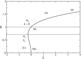
Figure 10: Mass $m$ of the DM particle as a function of the dimensionless self-interaction constant $\lambda$ in order to match the characteristics of the minimum halo. The mass is normalized by $m_{0}$ and the dimensionless self-interaction constant by $\lambda^{\prime}_{*}$. The stable part of the curve starts at the critical minimum halo point ($\lambda_{c},m_{c}$) which is also the minimum of the curve $\lambda(m)$.

Using Eqs. (74) and (188), the relation between the particle mass $m$ and the dimensionless self-interaction constant $\lambda$ required to match the characteristics of the minimum halo [see Eq. (72)] is given by

$$\lambda=\frac{8\pi aRm^{2}c}{b^{2}\hbar M}\left(\frac{GMm^{2}R}{a\hbar^{2}}-1\right).$$ (217)

Alternatively, using Eqs. (75) and (215), we obtain in dimensionless form

$$\frac{\lambda}{\lambda^{\prime}_{*}}=\left(\frac{m}{m_{0}}\right)^{2}\left[\left(\frac{m}{m_{0}}\right)^{2}-1\right].$$ (218)

This is a second degree equation whose solutions are

$$\frac{m}{m_{0}}=\left(\frac{1\pm\sqrt{1+4\lambda/\lambda^{\prime}_{*}}}{2}\right)^{1/2}$$ (219)

with the sign $+$ if $\lambda>0$ and the sign $\pm$ if $\lambda<0$. The curve $m(\lambda)$ is plotted in Fig. 10. Taking $a=9.946$ and $b=\pi$ (see Secs. III.1 and III.2) adapted to bosons with a repulsive self-interaction (or no interaction), we get $m_{0}=2.92\times 10^{-22}\,{\rm eV}/c^{2}$ and $\lambda^{\prime}_{*}=3.02\times 10^{-90}$. Taking $a=11.1$ and $b=5.5$ (see Sec. III.3) adapted to bosons with an attractive self-interaction, we get $m_{0}=3.08\times 10^{-22}\,{\rm eV}/c^{2}$ and $\lambda^{\prime}_{*}=1.23\times 10^{-90}$.

Remark: we note that the characteristic scale $\lambda^{\prime}_{*}\sim 10^{-90}$ is extremely small. We will see below that the NI limit is valid for $|\lambda|\ll\lambda^{\prime}_{*}$. Therefore, the dimensionless self-interaction constant $|\lambda|$ must be small with respect to $10^{-90}$, not with respect to $1$. For example, an apparently small value of $|\lambda|$ such as $|\lambda|=10^{-80}$ actually corresponds to a strong self-interaction. In other words, $|\lambda|=10^{-80}$ is very different from $\lambda=0$. The extraordinarily small value of $\lambda^{\prime}_{*}$ was first noted in prd2 (see also abrilphas ; phi6 ; bectcoll ; suarezchavanisprd3 ).

E.1 Noninteracting bosons

For noninteracting bosons ($\lambda=0$), we get

$$m_{0}=2.92\times 10^{-22}\,{\rm eV}/c^{2}\qquad({\rm BECNI})$$ (220)

E.2 Repulsive self-interaction

For bosons with a repulsive self-interaction ($\lambda>0$), $\lambda^{\prime}_{*}$ determines the transition between the NI regime ($\lambda\ll\lambda^{\prime}_{*}$) where $m\sim m_{0}$ and the TF regime ($\lambda\gg\lambda^{\prime}_{*}$) where

$$\frac{m}{m_{0}}\sim\left(\frac{\lambda}{\lambda^{\prime}_{*}}\right)^{1/4}.$$ (221)

When the self-interaction is repulsive, all the equilibrium states are stable. Therefore, in principle, all the values of $\lambda\geq 0$ and the corresponding masses $m\geq m_{0}$ are possible. In the TF regime, the $m(\lambda)$ relation (221) can be written as

$$\frac{\lambda}{8\pi m^{4}}\sim\frac{GR^{2}c}{b^{2}\hbar^{3}},$$ (222)

which is equivalent to Eq. (81). The minimum halo just determines the ratio

$$\frac{\lambda}{8\pi m^{4}}=1.66\times 10^{-5}\,({\rm eV}/c^{2})^{-4}.$$ (223)

Only the radius $R$ of the minimum halo matters in this determination. In order to determine $m$ and $\lambda$ individually, we need another equation. Repeating the argument from Sec. IV.2, the Bullet Cluster constraint implies that $\lambda$ must lie in the range $0\leq\lambda\leq\lambda_{\rm max}$ and that the particle mass must lie in the range $m_{0}\leq m\leq m_{\rm max}$ where

$$m_{\rm max}=1.10\times 10^{-3}\,{\rm eV}/c^{2},\quad\lambda_{\rm max}=6.18\times 10^{-16}$$

$$({\rm BECTF})\qquad$$ (224)

Although the value of $\lambda_{\rm max}=6.18\times 10^{-16}$ corresponding to the BECTF model may seem small, it is much larger than $\lambda^{\prime}_{*}=3.02\times 10^{-90}$, implying that we are deep into the TF regime (see the Remark above).

On the other hand, the BECt model corresponding to the transition between the NI limit and the TF limit, is obtained by substituting Eq. (220) into Eq. (221), or Eq. (79) into Eq. (222). This gives

$$m_{\rm t}=2.92\times 10^{-22}\,{\rm eV}/c^{2},\quad\lambda^{\prime}_{*}=3.02\times 10^{-90}$$

$$({\rm BECt})\qquad$$ (225)

This corresponds to the scales $m_{0}$ and $\lambda^{\prime}_{*}$ defined by Eqs. (76) and (216).

E.3 Attractive self-interaction in terms of $\lambda$

For bosons with an attractive self-interaction ($\lambda<0$), the relation (218) reveals the existence of a minimum value of the dimensionless self-interaction constant

$$\frac{\lambda_{c}}{\lambda^{\prime}_{*}}=-\frac{1}{4},\qquad{\rm at\quad which}\qquad\frac{m_{c}}{m_{0}}=\frac{1}{\sqrt{2}}.$$ (226)

It turns out that this minimum value also corresponds to the critical point (associated with the maximum mass $M_{\rm max}$) separating stable from unstable equilibrium states. The NI regime corresponds to $|\lambda|\ll\lambda^{\prime}_{*}$ and $m\sim m_{0}$. The NG regime corresponds to $|\lambda|\ll\lambda^{\prime}_{*}$ and $m\ll m_{0}$ such that

$$\frac{m}{m_{0}}\sim\left(\frac{|\lambda|}{\lambda^{\prime}_{*}}\right)^{1/2}.$$ (227)

In the NG regime, the relation (227) between $m$ and $\lambda$ can be written as

$$\frac{|\lambda|}{8\pi m^{2}}=\frac{a}{b^{2}}\frac{Rc}{M\hbar}=5.12\times 10^{-49}\,({\rm eV/c^{2}})^{-2},$$ (228)

which is equivalent to Eq. (68). The equilibrium states with $m<m_{c}$ are unstable (they correspond to configurations with $R<R_{*}$) so that only the equilibrium states with $m>m_{c}$ are stable (they correspond to configurations with $R>R_{*}$). Therefore, in the attractive case, the scattering length of the DM boson must lie in the range $\lambda_{c}<\lambda<0$ and its mass must lie in the range $m_{c}<m<m_{0}$, with

$$m_{\rm c}=2.19\times 10^{-22}\,{\rm eV}/c^{2},\quad\lambda_{c}=-3.07\times 10^{-91}$$

$$({\rm BECcrit})\qquad$$ (229)

There is no equilibrium state with $\lambda<\lambda_{c}$. Finally, using the constraints from particle physics and cosmology (see Sec. IV.4) we find

$$m_{\rm th}=2.92\times 10^{-22}\,{\rm eV}/c^{2},\quad\lambda_{\rm th}=-1.18\times 10^{-96}$$

$$({\rm BECth})\qquad$$ (230)

E.4 Attractive self-interaction in terms of $f$

The decay constant is defined by Eq. (189). This relation may be rewritten as

$$\frac{f}{f^{\prime}_{*}}=\left(\frac{m}{m_{0}}\right)^{1/2}\left(\frac{a^{\prime}_{*}}{|a_{s}|}\right)^{1/2},$$ (231)

where we have introduced the scales from Eqs. (76) and (77), and the new scale

$$f^{\prime}_{*}=\left(\frac{b^{2}}{a}\frac{\hbar c^{3}M}{32\pi R}\right)^{1/2}.$$ (232)

Using Eqs. (74) and (189), the relation between the particle mass and the decay constant is given by

$$\frac{1}{f^{2}}=\frac{32\pi aR}{b^{2}\hbar c^{3}M}\left(1-\frac{GMm^{2}R}{a\hbar^{2}}\right).$$ (233)

Alternatively, using Eqs. (75) and (231), we obtain in dimensionless form

$$\frac{m}{m_{0}}=\sqrt{1-\left(\frac{f^{\prime}_{*}}{f}\right)^{2}}.$$ (234)

The curve $m(f)$ is plotted in Fig. 11. Taking $a=11.1$ and $b=5.5$ (see Sec. III.3) adapted to bosons with an attractive self-interaction, we get $m_{0}=3.08\times 10^{-22}\,{\rm eV}/c^{2}$ and $f^{\prime}_{*}=1.39\times 10^{14}\,{\rm GeV}$.

Figure 11: Mass $m$ of the DM particle as a function of its decay constant $f$ in order to match the characteristics of the minimum halo. The mass is normalized by $m_{0}$ and the decay constant by $f^{\prime}_{*}$. The stable part of the curve starts at the critical minimum halo point ($f_{c},m_{c}$). It differs from the absolute minimum value $f_{\rm min}$ of the decay constant.

The relation from Eq. (234) reveals the existence of a minimum decay constant $f_{\rm min}=f^{\prime}_{*}=1.39\times 10^{14}\,{\rm GeV}$ at which $m=0$. However, this minimum scattering length $f_{\rm min}$ does not correspond to the critical point (associated with the maximum mass $M_{\rm max}$) separating stable from unstable equilibrium states. This latter is located at

$$\frac{f_{c}}{f^{\prime}_{*}}=\sqrt{2},\qquad\frac{m_{c}}{m_{0}}=\frac{1}{\sqrt{2}}.$$ (235)

The NI regime corresponds to $f\gg f_{\rm min}$ and $m\sim m_{0}$. The NG regime corresponds to $f\sim f_{\rm min}$ and $m\ll m_{0}$.

The equilibrium states with $m<m_{c}$ are unstable (they correspond to configurations with $R<R_{*}$) so that only the equilibrium states with $m>m_{c}$ are stable (they correspond to configurations with $R>R_{*}$). Therefore, the decay constant of the DM boson must lie in the range $f>f_{c}$ and its mass must lie in the range $m_{c}<m<m_{0}$, with

$$m_{\rm c}=2.19\times 10^{-22}\,{\rm eV}/c^{2},\quad f_{c}=1.97\times 10^{14}\,{\rm GeV}$$

$$({\rm BECcrit})\qquad$$ (236)

There is no equilibrium state with $f<f_{\rm min}$. On the other hand, the equilibrium states with $f_{\rm min}\leq f<f_{c}$ are unstable. Using the constraints from particle physics and cosmology (see Sec. IV.4) we find

$$m_{\rm th}=2.92\times 10^{-22}\,{\rm eV}/c^{2},\quad f_{\rm th}=1.34\times 10^{17}\,{\rm GeV}$$

$$({\rm BECth})\qquad$$ (237)

We note that $f_{\rm th}<M_{P}c^{2}=1.22\times 10^{19}\,{\rm GeV}$.

Appendix F Pulsation of self-gravitating BECs

F.1 General case

The square pulsation of the standard self-gravitating BEC is approximately given by (see Appendix G.2)

$$\omega^{2}=\frac{6\Theta_{Q}+12U+2W}{I}.$$ (238)

This equation can be written in different forms by using the virial theorem $2\Theta_{Q}+3U+W=0$ (see Sec. II.2).

With the $f$-ansatz (see Appendix G.2), the square pulsation is given by

$$\omega^{2}=\frac{6\sigma}{\alpha}\frac{\hbar^{2}}{m^{2}R^{4}}-\frac{2\nu}{\alpha}\frac{GM}{R^{3}}+\frac{24\pi\zeta}{\alpha}\frac{a_{s}\hbar^{2}M}{m^{3}R^{5}}.$$ (239)

On the other hand, the mass-radius relation writes

$$-2\sigma\frac{\hbar^{2}M}{m^{2}R^{3}}+\nu\frac{GM^{2}}{R^{2}}-6\pi\zeta\frac{a_{s}\hbar^{2}M^{2}}{m^{3}R^{4}}=0$$ (240)

or, equivalently,

$$M=\frac{\frac{2\sigma}{\nu}\frac{\hbar^{2}}{Gm^{2}R}}{1-\frac{6\pi\zeta}{\nu}\frac{a_{s}\hbar^{2}}{Gm^{3}R^{2}}}.$$ (241)

If we use a Gaussian ansatz, the values of the coefficients are $\alpha_{\rm G}=3/2$, $\sigma_{\rm G}=3/4$, $\zeta_{\rm G}=1/(2\pi)^{3/2}$, and $\nu_{\rm G}=1/\sqrt{2\pi}$ prd1 . Furthermore, the relation between the radius $R$ and the radius $R_{99}$ containing $99\%$ of the mass is $R_{99}=2.38167\,R$ prd1 . The square pulsation is plotted as a function of the BEC radius $R$ in prd1 .

F.2 Noninteracting case

For noninteracting bosons ($a_{s}=0$), the square pulsation from Eq. (238) reduces to

$$\omega^{2}=\frac{6\Theta_{Q}+2W}{I}=\frac{2\Theta_{Q}}{I}=-\frac{W}{I},$$ (242)

where we have used the virial theorem $2\Theta_{Q}+W=0$ to get the last two equalities.

With the $f$-ansatz, the square pulsation is given by

$$\omega^{2}=\frac{6\sigma}{\alpha}\frac{\hbar^{2}}{m^{2}R^{4}}-\frac{2\nu}{\alpha}\frac{GM}{R^{3}}.$$ (243)

On the other hand, the mass-radius relation writes

$$R=\frac{2\sigma}{\nu}\frac{\hbar^{2}}{GMm^{2}}.$$ (244)

Combining these two relations we obtain

$$\omega^{2}=\frac{\nu}{\alpha}\frac{GM}{R^{3}}=\frac{2\sigma}{\alpha}\frac{\hbar^{2}}{m^{2}R^{4}}=\frac{\nu^{4}}{8\alpha\sigma^{3}}\frac{G^{4}M^{4}m^{6}}{\hbar^{6}}.$$ (245)

If we use a Gaussian ansatz, the prefactors are $0.266$, $1$ and $5.00\times 10^{-3}$. The first relation of Eq. (245) shows that the pulsation period $T=2\pi/\omega$ is about $12.2$ dynamical times $t_{d}=(R^{3}/GM)^{1/2}$. For the minimum halo with $M=10^{8}\,M_{\odot}$ and $R=(1/2.38167)\,{\rm kpc}$, we get $t_{d}=12.8\,{\rm Myrs}$ and $T=156\,{\rm Myrs}$.

F.3 TF limit

For bosons with a repulsive self-interaction ($a_{s}>0$) in the TF limit ($\hbar=0$), the square pulsation from Eq. (238) reduces to

$$\omega^{2}=\frac{12U+2W}{I}=\frac{6U}{I}=-\frac{2W}{I},$$ (246)

where we have used the virial theorem $3U+W=0$ to get the last two equalities.

With the $f$-ansatz, the square pulsation is given by

$$\omega^{2}=-\frac{2\nu}{\alpha}\frac{GM}{R^{3}}+\frac{24\pi\zeta}{\alpha}\frac{a_{s}\hbar^{2}M}{m^{3}R^{5}}.$$ (247)

On the other hand, the radius of the BEC is

$$R=\left(\frac{6\pi\zeta}{\nu}\right)^{1/2}\left(\frac{a_{s}\hbar^{2}}{Gm^{3}}\right)^{1/2}.$$ (248)

Combining these two relations we obtain

$$\omega^{2}=\frac{2\nu}{\alpha}\frac{GM}{R^{3}}=\frac{2\nu^{5/2}}{\alpha(6\pi\zeta)^{3/2}}\frac{G^{5/2}Mm^{9/2}}{a_{s}^{3/2}\hbar^{3}}.$$ (249)

If we use a Gaussian ansatz, the prefactors are $0.532$ and $0.102$. The pulsation period $T=2\pi/\omega$ is about $8.62$ dynamical times $t_{d}=(R^{3}/GM)^{1/2}$. For the minimum halo with $M=10^{8}\,M_{\odot}$ and $R=(1/2.38167)\,{\rm kpc}$, we get $t_{d}=12.8\,{\rm Myrs}$ and $T=111\,{\rm Myrs}$.

Remark: In the TF approximation, the density profile of the BECDM halo is known analytically. In that case, one can obtain the exact expression of the pulsation (see prd1 and Appendices H and I of epjpbh ).

F.4 Maximum mass and maximum pulsation

For bosons with an attractive self-interaction ($a_{s}<0$), the pulsation vanishes at the maximum mass prd1 :

$$\omega=0\quad{\rm at}\quad M=M_{\rm max}.$$ (250)

With the $f$-ansatz:

$$M_{\rm max}=\left(\frac{\sigma^{2}}{6\pi\zeta\nu}\right)^{1/2}\frac{\hbar}{\sqrt{Gm|a_{s}|}},$$ (251)

$$R_{*}=\left(\frac{6\pi\zeta}{\nu}\right)^{1/2}\left(\frac{|a_{s}|\hbar^{2}}{Gm^{3}}\right)^{1/2}.$$ (252)

On the other hand, there is a maximum pulsation at some ${\tilde{M}}<M_{\rm max}$ prd1 . With the $f$-ansatz:

$$\omega_{\rm max}=0.4246\,\frac{\nu}{6\pi\zeta}\sqrt{\frac{\sigma}{\alpha}}\frac{Gm^{2}}{|a_{s}|\hbar}$$ (253)

at

$${\tilde{M}}=0.9717\,M_{\rm max},\qquad{\tilde{R}}=1.272\,R_{*}.$$ (254)

F.5 Nongravitational case

For bosons with an attractive self-interaction ($a_{s}<0$) in the NG limit ($G=0$), the square pulsation from Eq. (238) reduces to

$$\omega^{2}=\frac{6\Theta_{Q}+12U}{I}=-\frac{2\Theta_{Q}}{I}=\frac{3U}{I},$$ (255)

where we have used the virial theorem $2\Theta_{Q}+3U=0$ to get the last two equalities.

With the $f$-ansatz, the square pulsation is given by

$$\omega^{2}=\frac{6\sigma}{\alpha}\frac{\hbar^{2}}{m^{2}R^{4}}+\frac{24\pi\zeta}{\alpha}\frac{a_{s}\hbar^{2}M}{m^{3}R^{5}}.$$ (256)

On the other hand, the mass-radius relation writes

$$M=\frac{\sigma}{3\pi\zeta}\frac{mR}{|a_{s}|}.$$ (257)

Combining these two relations we obtain

$$\omega^{2}=-\frac{2\sigma}{\alpha}\frac{\hbar^{2}}{m^{2}R^{4}}=-\frac{2\sigma^{5}}{\alpha(3\pi\zeta)^{4}}\frac{m^{2}\hbar^{2}}{M^{4}a_{s}^{4}}.$$ (258)

If we use a Gaussian ansatz, the prefactors are $1$ and $2.47$. Note that these configurations are unstable ($\omega^{2}<0$) so they should not be observed in practice.

Appendix G Similarity between the mass-radius relation obtained from the $f$-ansatz and from the Jeans instability study

In this Appendix, we show at a general level that the mass-radius relation $M_{J}(R_{J})$ obtained from the Jeans instability study is similar to the mass-radius relation $M(R)$ of DM halos in their ground state obtained from the minimization of the energy at fixed mass using an $f$-ansatz. This similarity was first observed in Ref. prd1 in a special case (for a $|\psi|^{4}$ potential of interaction and for a Gaussian ansatz) and it is here generalized to an arbitrary potential of interaction $V(|\psi|^{2})$ and an arbitrary ansatz.

G.1 Mass-radius relation from the Jeans instability study

In this section, we consider the formation of structures in the linear regime from the Jeans instability study (see Sec. II.4). The Jeans wavenumber is determined by the equation prd1

$$\frac{\hbar^{2}k_{J}^{4}}{4m^{2}}+c_{s}^{2}k_{J}^{2}-4\pi G\rho=0,$$ (259)

where $c_{s}^{2}$ is the square of the speed of sound. For a barotropic fluid, this is a function of the density given by Eq. (17). Eq. (259) is a second degree equation for $k_{J}^{2}$ whose physical solution is

$$k_{J}^{2}=\frac{2m^{2}}{\hbar^{2}}\left[-c_{s}^{2}(\rho)+\sqrt{c_{s}^{4}(\rho)+\frac{4\pi G\rho\hbar^{2}}{m^{2}}}\right].$$ (260)

If we define the Jeans radius and the Jeans mass by

$$R_{J}=\frac{\lambda_{J}}{2}=\frac{\pi}{k_{J}},\qquad M_{J}=\frac{4}{3}\pi\rho R_{J}^{3},$$ (261)

we obtain

$$R_{J}(\rho)=\frac{\frac{\pi\hbar}{\sqrt{2}m}}{\left[-c_{s}^{2}(\rho)+\sqrt{c_{s}^{4}(\rho)+\frac{4\pi G\rho\hbar^{2}}{m^{2}}}\right]^{1/2}},$$ (262)

$$M_{J}(\rho)=\frac{4}{3}\pi\rho R_{J}(\rho)^{3}.$$ (263)

These equations determine the Jeans scales $R_{J}(\rho)$ and $M_{J}(\rho)$ as a function of the density. They also determine the Jeans mass-radius relation $M_{J}(R_{J})$ in parametric form with parameter $\rho$.

Remark: In the nongravitational case, there is a hydrodynamic instability when $c_{s}^{2}<0$ khlopov ; prd1 . In that case, the “Jeans” wavenumber is determined by the equation

$$\frac{\hbar^{2}k_{J}^{2}}{4m^{2}}+c_{s}^{2}=0,$$ (264)

and the parametric equations (262) and (263) reduce to

$$R_{J}(\rho)=\frac{\pi\hbar}{2m\sqrt{-c_{s}^{2}(\rho)}},$$ (265)

$$M_{J}(\rho)=\frac{4}{3}\pi\rho R_{J}(\rho)^{3}.$$ (266)

G.2 Mass-radius relation from the $f$-ansatz

In this section, we consider BECDM halos that appear in the nonlinear regime of structure formation (see Sec. II.3). Stable DM halos correspond to minima of energy $E_{\rm min}$ at fixed mass $M$. We can obtain an approximate analytical form of the mass-radius relation by making an ansatz for the wave function. A Gaussian ansatz was considered in prd1 . To be as general as possible, we consider here an ansatz of the form (that we call $f$-ansatz)

$$\rho({\bf r},t)=\frac{M}{R(t)^{3}}f\left[\frac{\bf r}{R(t)}\right],$$ (267)

where $f({\bf x})$ is an arbitrary function. We impose $\int f({\bf x})\,d{\bf x}=1$ to satisfy the normalization condition (or the conservation of mass). We also assume

$$S({\bf r},t)=\frac{1}{2}mH(t)r^{2}\quad\Rightarrow\quad{\bf u}({\bf r},t)=H(t){\bf r},$$ (268)

so that the velocity field is proportional to the radial distance. It can be shown (see Appendix J of ggpp ) that Eqs. (267) and (268) yield an exact solution of the continuity equation (10) provided that

$$H=\frac{\dot{R}}{R}.$$ (269)

This function is similar to the Hubble parameter in cosmology. On the other hand, the gravitational potential can be determined from the Poisson equation (13). Using Eq. (267) we obtain

$$\Phi({\bf r},t)=\frac{GM}{R(t)}g\left[\frac{\bf r}{R(t)}\right],$$ (270)

where $g({\bf x})$ is the solution of

$$\Delta g=4\pi f({\bf x}).$$ (271)

We can now use the ansatz (267)-(271) to determine the different functionals that appear in the energy from Eq. (21). We find

$$\Theta_{c}=\frac{1}{2}\alpha M\left(\frac{dR}{dt}\right)^{2}\quad{\rm with}\quad\alpha=\int f({\bf x})x^{2}\,d{\bf x},$$ (272)

$$\Theta_{Q}=\sigma\frac{\hbar^{2}M}{m^{2}R^{2}}\quad{\rm with}\quad\sigma=\frac{1}{8}\int\frac{(\nabla f)^{2}}{f}\,d{\bf x},$$ (273)

$$U=\frac{\zeta}{\gamma-1}\frac{KM^{\gamma}}{R^{3(\gamma-1)}}\quad{\rm with}\quad\zeta=\int f^{\gamma}({\bf x})\,d{\bf x},$$ (274)

and

$$W=-\nu\frac{GM^{2}}{R}\quad{\rm with}\quad\nu=-\frac{1}{2}\int f({\bf x})g({\bf x})\,d{\bf x}.$$ (275)

The expression (274) of the internal energy $U$ is valid for a power-law potential associated with a polytropic equation of state (we will see later how to generalize the formalism to an arbitrary potential of interaction or an arbitrary equation of state). The moment of inertia is

$$I=\alpha MR^{2}.$$ (276)

If we use a Gaussian ansatz $f({\bf x})=\frac{1}{\pi^{3/2}}e^{-x^{2}}$, the values of the coefficients are $\alpha_{\rm G}=3/2$, $\sigma_{\rm G}=3/4$, $\zeta_{\rm G}=1/(\gamma\pi^{\gamma-1})^{3/2}$, and $\nu_{\rm G}=1/\sqrt{2\pi}$ prd1 .

With the ansatz from Eqs. (267) and (268) the total energy can be written as

$$E_{\rm tot}=\frac{1}{2}\alpha M\left(\frac{dR}{dt}\right)^{2}+V(R)$$ (277)

with

$$V(R)=\sigma\frac{\hbar^{2}M}{m^{2}R^{2}}-\nu\frac{GM^{2}}{R}+\frac{\zeta}{\gamma-1}\frac{KM^{\gamma}}{R^{3(\gamma-1)}}.$$ (278)

We have separated the classical kinetic energy $\Theta_{c}$ from the potential energy $V=\Theta_{Q}+U+W$. From the conservation of energy, $\dot{E}_{\rm tot}=0$, we obtain

$$\alpha M\frac{d^{2}R}{dt^{2}}=-V^{\prime}(R).$$ (279)

This is similar to the equation of motion of a fictive particle of mass $\alpha M$ and position $R$ moving in a potential $V(R)$. At equilibrium, the condition $V^{\prime}(R)=0$ (extremum of energy) gives the mass-radius relation

$$-2\sigma\frac{\hbar^{2}M}{m^{2}R^{3}}+\nu\frac{GM^{2}}{R^{2}}-3\zeta\frac{KM^{\gamma}}{R^{3(\gamma-1)+1}}=0.$$ (280)

For the standard BEC, we get Eq. (240). The foregoing equations may also be obtained from the virial theorem prd1 ; ggpp or from the Lagrange equations bectcoll ; ggpp .

The pulsation of the self-gravitating BEC is given by prd1 ; ggpp

$$\omega^{2}=\frac{1}{\alpha M}V^{\prime\prime}(R).$$ (281)

The BEC is stable provides that $\omega^{2}>0$ which is equivalent by Eq. (281) to the requirement that the equilibrium state is a minimum of energy. Using Eq. (278) we obtain

$$\omega^{2}=\frac{6\sigma}{\alpha}\frac{\hbar^{2}}{m^{2}R^{4}}-\frac{2\nu}{\alpha}\frac{GM}{R^{3}}+[3(\gamma-1)+1]\frac{3\zeta}{\alpha}\frac{KM^{\gamma-1}}{R^{3(\gamma-1)+2}}.$$ (282)

Using Eqs. (273)-(276), the pulsation can also be written in terms of the BEC functionals as

$$\omega^{2}=\frac{6\Theta_{Q}+[3(\gamma-1)+1]3(\gamma-1)U+2W}{I}.$$ (283)

For the usual BEC, we obtain Eqs. (238) and (239).

In order to compute the internal energy $U$ for a general self-interaction potential we consider an ansatz based on a uniform (top-hat) density

$$\rho({\bf r},t)=\frac{3M}{4\pi R(t)^{3}}\theta(|{\bf r}|-R(t)),$$ (284)

where $\theta$ is the Heaviside function ($\theta(x)=1$ if $x<0$ and $\theta(x)=0$ if $x>0$). In that case, the internal energy is given by

$$U=V\left(\frac{3M}{4\pi R^{3}}\right)\frac{4}{3}\pi R^{3}.$$ (285)

We then find that

$$U^{\prime}(R)=\frac{d}{dR}\left[\frac{V(\rho)}{\rho}M\right]=M\frac{d}{d\rho}\left[\frac{V(\rho)}{\rho}\right]\frac{d\rho}{dR}$$

$$=-\frac{9M^{2}}{4\pi R^{4}}\frac{d}{d\rho}\left[\frac{V(\rho)}{\rho}\right].$$ (286)

Using Eq. (15) which corresponds to the first principle of thermodynamics (see Appendix H)

$$\left[\frac{V(\rho)}{\rho}\right]^{\prime}=\frac{P(\rho)}{\rho^{2}}\quad\Leftrightarrow\quad d\left(\frac{V}{\rho}\right)=-Pd\left(\frac{1}{\rho}\right),$$ (287)

we obtain

$$U^{\prime}(R)=-P\left(\frac{3M}{4\pi R^{3}}\right)4\pi R^{2}\quad\Leftrightarrow\quad dU=-P\,d{\cal V},$$ (288)

where ${\cal V}=(4/3)\pi R^{3}$ denotes the volume of the BEC. For a power-law self-interaction potential, we recover the expression of $U$ from Eq. (274) with a coefficient $\zeta_{\rm C}=(3/4\pi)^{\gamma-1}$. On the other hand, the coefficients entering in the expressions of $\Theta_{c}$ and $W$ from Eqs. (272) and (275) are $\alpha_{\rm C}=3/5$ and $\nu_{\rm C}=3/5$. Unfortunately, we cannot use the constant density ansatz to determine the quantum kinetic energy $\Theta_{c}$ since it is produced by the gradient of the density which is infinite for the top-hat profile.

For an arbitrary self-interaction potential, we can write the total energy as in Eq. (277) with an approximate potential energy given by

$$V(R)=\sigma\frac{\hbar^{2}M}{m^{2}R^{2}}-\nu\frac{GM^{2}}{R}+\chi V\left(\frac{3M}{4\pi R^{3}}\right)\frac{4}{3}\pi R^{3},$$ (289)

where $\chi$ is a tunable coefficient. For a power-law self-interaction potential, we exactly recover Eq. (278) with $\chi=\zeta\left({4\pi}/{3}\right)^{\gamma-1}$. For an arbitrary self-interaction potential, using Eqs. (288) and (289), we get

$$V^{\prime}(R)=-2\sigma\frac{\hbar^{2}M}{m^{2}R^{3}}+\nu\frac{GM^{2}}{R^{2}}-\chi P\left(\frac{3M}{4\pi R^{3}}\right)4\pi R^{2}.$$ (290)

The condition of equilibrium $V^{\prime}(R)=0$ then yields the mass-radius relation under the form

$$-2\sigma\frac{\hbar^{2}M}{m^{2}R^{3}}+\nu\frac{GM^{2}}{R^{2}}-\chi P\left(\frac{3M}{4\pi R^{3}}\right)4\pi R^{2}=0.$$ (291)

If we work with the variables $M$ and $R$ it is usually difficult to solve this equation explicitly in the general case. However, if we make the change of variables

$$R=\frac{\pi}{k},\qquad M=\frac{4}{3}\pi\rho R^{3},$$ (292)

inspired by Eq. (261), we get

$$\frac{2\sigma}{\pi^{2}}\frac{\hbar^{2}k^{4}}{m^{2}}+3\chi\frac{P(\rho)}{\rho}k^{2}-\frac{4}{3}\pi^{3}\nu G\rho=0.$$ (293)

Remarkably, this equation is similar to the Jeans equation (259). Therefore, it can be solved easily (this is just a second degree equation for $k^{2}$) and the mass-radius relation $M(R)$ can be obtained in parametric form as in Appendix G.1. We get

$$R(\rho)=\frac{\frac{2\sqrt{\sigma}\hbar}{m}}{\left[-3\chi\frac{P(\rho)}{\rho}+\sqrt{9\chi^{2}\frac{P(\rho)^{2}}{\rho^{2}}+\frac{32\pi}{3}\sigma\nu\frac{G\rho\hbar^{2}}{m^{2}}}\right]^{1/2}},$$ (294)

$$M(\rho)=\frac{4}{3}\pi\rho R(\rho)^{3}.$$ (295)

This shows in full generality that the Jeans mass-radius relation $M_{J}(R_{J})$ valid in the linear regime of structure formation is formally similar to the mass-radius relation $M(R)$ of DM halos valid in the nonlinear regime of structure formation. Apart from the precise value of the prefactors, we see that the difference with the Jeans study is that the pressure derivative $P^{\prime}(\rho)$ (appearing in $c_{s}^{2}$) is replaced by the ratio $P(\rho)/\rho$. For a polytropic equation of state, the dependence in the density is the same, i.e., $\rho^{\gamma-1}$ but the prefactor is different.

Appendix H Thermodynamical identities for cold barotropic gases

In this Appendix, we regroup useful thermodynamical identities valid for cold barotropic gases.

The first principle of thermodynamics can be written under a local form as

$$d\left(\frac{u}{\rho}\right)=-Pd\left(\frac{1}{\rho}\right)+Td\left(\frac{s}{\rho}\right),$$ (296)

where $u$ is the density of internal energy, $\rho$ is the mass density, $P$ is the pressure, $T$ is the temperature and $s$ is the entropy density. For cold gases ($T=0$), Eq. (296) reduces to

$$d\left(\frac{u}{\rho}\right)=-Pd\left(\frac{1}{\rho}\right)=\frac{P}{\rho^{2}}d\rho.$$ (297)

If we introduce the enthalpy density

$$h=\frac{P+u}{\rho},$$ (298)

we obtain the relations

$$du=h\,d\rho\qquad{\rm and}\qquad dh=\frac{dP}{\rho}.$$ (299)

We also recall that, according to the Gibbs-Duhem relation for a cold gas ($T=0$), the local chemical potential coincides with the enthalpy ($h=\mu_{\rm loc}/m$).

H.1 General barotropic equation of state

For a general barotropic equation of state of the form $P=P(\rho)$, the foregoing relations lead to the identities

$$\left(\frac{u}{\rho}\right)^{\prime}=\frac{P(\rho)}{\rho^{2}},$$ (300)

$$h(\rho)=u^{\prime}(\rho),$$ (301)

$$h^{\prime}(\rho)=\frac{P^{\prime}(\rho)}{\rho},$$ (302)

$$P(\rho)=\rho h(\rho)-u(\rho)=\rho u^{\prime}(\rho)-u(\rho)=\rho^{2}\left(\frac{u}{\rho}\right)^{\prime},$$ (303)

$$P^{\prime}(\rho)=\rho u^{\prime\prime}(\rho).$$ (304)

The first principle of thermodynamics for a barotropic gas at $T=0$ [see Eq. (297)] provides a general relation between the density of internal energy $u(\rho)$ and the pressure $P(\rho)$. If we know the energy density $u=u(\rho)$, we can obtain the pressure by

$$P=-\frac{d(u/\rho)}{d(1/\rho)}=\rho\frac{du}{d\rho}-u.$$ (305)

Inversely, if we know the equation of state $P=P(\rho)$, we can obtain the energy density by

$$u(\rho)=\rho\int^{\rho}\frac{P(\rho^{\prime})}{{\rho^{\prime}}^{2}}\,d\rho^{\prime}.$$ (306)

Remark: Comparing Eqs. (15) and (16) with Eqs. (303) and (304), we see that the potential $V(\rho)$ that occurs in the GP equation (1) represents the density of internal energy:

$$u(\rho)=V(\rho).$$ (307)

This justifies the expression of the internal energy in Eqs. (7) and (24).

H.2 Polytropic equation of state

For a polytropic equation of state of the form $P=K\rho^{\gamma}$ with $\gamma=1+1/n$, the density of internal energy [see Eq. (306)] is explicitly given by

$$u=\frac{K}{\gamma-1}\rho^{\gamma}=\frac{P}{\gamma-1}=nP=nK\rho^{1+1/n},$$ (308)

where we have set the constant of integration to zero. For the standard BEC corresponding to $\gamma=2$ [see Eq. (3)], we have

$$u=P=\frac{2\pi a_{s}\hbar^{2}}{m^{3}}\rho^{2}\quad\Rightarrow\quad U=\frac{2\pi a_{s}\hbar^{2}}{m^{3}}\int\rho^{2}\,d{\bf r}.$$ (309)

Appendix I Derivation of the GPP equations in an expanding Universe

In this Appendix, proceeding as in Ref. aacosmo , we derive the GPP equations in an expanding universe starting from their expression in the inertial frame. Alternative derivations, starting directly from the KGE equations written with the conformal Newtonian gauge which is a perturbed form of the Friedmann-Lemaître-Robertson-Walker (FLRW) metric accounting for the expansion of the Universe, and taking the nonrelativistic limit $c\rightarrow+\infty$, can be found in Refs. abrilph ; playa ; chavmatos ; phi6 .

I.1 Homogeneous solution

In the inertial frame, the GPP equations are given by Eqs. (1) and (2). The corresponding hydrodynamic equations, obtained from the Madelung madelung transformation, are given by Eqs. (10)-(13). Let us first show that these equations admit a time-dependent spatially homogeneous solution describing an expanding universe in a Newtonian cosmology.

We consider a spatially homogeneous solution of Eqs. (10)-(13) of the form

$$\rho_{b}({\bf r},t)=\rho_{b}(t),\qquad S_{b}({\bf r},t)=\frac{1}{2}H(t)mr^{2}+S_{0}(t),$$ (310)

$${\bf u}_{b}({\bf r},t)=H(t){\bf r},\qquad\Phi_{b}({\bf r},t)=\frac{2}{3}\pi G\rho_{b}(t)r^{2},$$ (311)

where $a(t)$ is the scale factor and $H=\dot{a}/a$ is the Hubble constant (actually a function of time). The velocity is assumed to be proportional to the distance (Hubble’s law) and the gravitational potential has been determined from the Poisson equation $\Delta\Phi_{b}=4\pi G\rho_{b}$. The corresponding wavefunction is

$$\psi_{b}({\bf r},t)=\sqrt{\rho_{b}(t)}e^{i\left[\frac{1}{2}H(t)mr^{2}+S_{0}(t)\right]/\hbar}.$$ (312)

The hydrodynamic equations (10)-(13) then reduce to

$$\frac{d\rho_{b}}{dt}+3H\rho_{b}=0\qquad\Rightarrow\qquad\rho_{b}\propto a^{-3},$$ (313)

$$\frac{dS_{0}}{dt}=-mV^{\prime}(\rho_{b}),$$ (314)

$$\dot{H}+H^{2}=-\frac{4}{3}\pi G\rho_{b}\qquad\Rightarrow\qquad\ddot{a}=-\frac{4}{3}\pi G\rho_{b}a.$$ (315)

The first equation can be interpreted as the conservation of mass

$$M=\frac{4}{3}\pi\rho_{b}a^{3}\qquad\Rightarrow\qquad\rho_{b}=\frac{3M}{4\pi a^{3}}$$ (316)

and the third equation as the Newtonian equation of dynamics

$$\ddot{a}=-\frac{GM}{a^{2}}=-\frac{\frac{4}{3}\pi G\rho_{b}a^{3}}{a^{2}}$$ (317)

for a particle submitted to a gravitational field $-{GM}/{a^{2}}$ created by a mass $M$. These equations can be justified in a Newtonian cosmology if we view the Universe as a homogeneous sphere of mass $M$, radius $a(t)$ and density $\rho_{b}(t)$ evolving under its own gravitation. Eq. (317) is then obtained by considering the force experienced by a particle of arbitrary mass $m$ on the surface of this sphere and using Newton’s law. The first integral of motion is

$$\frac{1}{2}\left(\frac{da}{dt}\right)^{2}-\frac{GM}{a}=E$$ (318)

implying

$$\left(\frac{da}{dt}\right)^{2}=\frac{2GM}{a}+2E=\frac{8}{3}\pi G\rho_{b}a^{2}+2E.$$ (319)

We can check that the foregoing equations coincide with the Friedmann equations in the nonrelativistic limit (or for pressureless matter). In the context of general relativity, the term $-2E$ represents the curvature of space $\kappa$, where $\kappa=-1,0,+1$ depending whether the Universe is open, critical, or closed. The theory of inflation and the observations of the CMB favor a flat universe ($\kappa=0$) so we shall take $E=0$. In that case, Eq. (319) reduces to

$$\left(\frac{da}{dt}\right)^{2}=\frac{8}{3}\pi G\rho_{b}a^{2}\qquad\Rightarrow\qquad H^{2}=\frac{8}{3}\pi G\rho_{b}.$$ (320)

Combining Eq. (320) with Eq. (313) we obtain the solution

$$a\propto t^{2/3},\qquad H=\frac{\dot{a}}{a}=\frac{2}{3t},\qquad\rho_{b}=\frac{1}{6\pi Gt^{2}},$$ (321)

which corresponds to the Einstein-de Sitter (EdS) universe (we have assumed a vanishing cosmological constant $\Lambda=0$).

I.2 Comoving frame

We now write the GPP equations in the comoving frame. To that purpose, we make the change of variables

$${\bf r}=a(t){\bf x},\qquad\psi({\bf r},t)=\Psi({\bf x},t)e^{i\frac{1}{2}mHr^{2}/\hbar},$$ (322)

where ${\bf r}$ is the proper distance. Eq. (322) is a change of variables from proper locally Minkowski coordinates ${\bf r}$ to expanding coordinates ${\bf x}$ comoving in the background model peeblesbook . The density is given by $\rho=|\Psi|^{2}$. Defining the gravitational potential $\phi({\bf x},t)$ by

$$\Phi({\bf r},t)=\Phi_{b}({\bf r},t)+\phi({\bf x},t),$$ (323)

we find that the Poisson equation (13) becomes

$$\Delta\phi=4\pi Ga^{2}(\rho-\rho_{b}),$$ (324)

where the derivatives are with respect to ${\bf x}$ (the same is true for the following equations unless explicitly stated).

In order to transform the GPP equations (1) and (2) to the comoving frame we first compute

$$\left(\frac{\partial\psi}{\partial t}\right)_{\bf r} = \left(\frac{\partial}{\partial t}\right)_{\bf r}\Psi\left(\frac{{\bf r}}{a(t)},t\right)e^{i\frac{1}{2}mHr^{2}/\hbar}$$

$$= \left(\frac{\partial\Psi}{\partial t}-H{\bf x}\cdot\nabla\Psi+\frac{i}{2\hbar}m{\dot{H}}a^{2}x^{2}\Psi\right)e^{i\frac{1}{2}mHr^{2}/\hbar},$$

and

$$\Delta_{\bf r}\psi=\biggl{(}\frac{1}{a^{2}}\Delta\Psi+3\frac{i}{\hbar}mH\Psi+2\frac{i}{\hbar}mH{\bf x}\cdot\nabla\Psi$$

$$-\frac{m^{2}H^{2}}{\hbar^{2}}a^{2}x^{2}\Psi\biggr{)}e^{i\frac{1}{2}mHr^{2}/\hbar}.$$ (326)

Substituting the foregoing relations into Eq. (1) we find after simplification (using Eq. (315)) that

$$i\hbar\frac{\partial\Psi}{\partial t}+\frac{3}{2}i\hbar H\Psi=-\frac{\hbar^{2}}{2ma^{2}}\Delta\Psi+m\frac{dV}{d|\Psi|^{2}}\Psi+m\phi\Psi.$$ (327)

On the other hand, using Eq. (320), the Poisson equation (324) can be written as

$$\frac{\Delta\phi}{4\pi Ga^{2}}=|\Psi|^{2}-\frac{3H^{2}}{8\pi G}.$$ (328)

We can similarly transform the hydrodynamic equations (10)-(13) to the comoving frame. The wave function can be written as

$$\Psi({\bf x},t)=\sqrt{{\rho({\bf x},t)}}e^{i{\cal S}({\bf x},t)/\hbar},$$ (329)

where $\rho({\bf x},t)$ is the mass density and ${\cal S}({\bf x},t)$ is the action in the comoving frame. Making the Madelung madelung transformation

$$\rho({\bf x},t)=|\Psi|^{2}\qquad{\rm and}\qquad{\bf v}=\frac{\nabla{\cal S}}{ma},$$ (330)

where ${\bf v}({\bf x},t)$ is the velocity field in the comoving frame, and comparing Eqs. (8), (322) and (329), we get

$$S({\bf r},t)={\cal S}({\bf x},t)+\frac{1}{2}mHr^{2}\quad\Rightarrow\quad{\bf u}({\bf r},t)={\bf v}({\bf x},t)+H{\bf r},$$ (331)

where ${\bf u}$ is the velocity field in the inertial frame and $H{\bf r}$ is the Hubble flow. Then, we compute

$$\left(\frac{\partial\rho}{\partial t}\right)_{\bf r}=\left(\frac{\partial}{\partial t}\right)_{\bf r}\rho\left(\frac{{\bf r}}{a(t)},t\right)=\frac{\partial\rho}{\partial t}-H{\bf x}\cdot\nabla\rho$$ (332)

and

$$\nabla_{\bf r}(\rho{\bf u})=\frac{1}{a}\nabla\cdot(\rho{\bf v})+H{\bf x}\cdot\nabla\rho+3H\rho.$$ (333)

With these relations, the continuity equation (10) becomes

$$\frac{\partial\rho}{\partial t}+3H\rho+\frac{1}{a}\nabla\cdot(\rho{\bf v})=0.$$ (334)

Similarly, using

$$\left(\frac{\partial{\bf u}}{\partial t}\right)_{\bf r}=\left(\frac{\partial}{\partial t}\right)_{\bf r}{\bf v}\left(\frac{{\bf r}}{a(t)},t\right)+\dot{H}{\bf r}=\frac{\partial{\bf v}}{\partial t}-H({\bf x}\cdot\nabla){\bf v}+\dot{H}a{\bf x},$$ (335)

and

$$({\bf u}\cdot\nabla_{\bf r}){\bf u} = \left[(H{\bf r}+{\bf v})\cdot\nabla_{\bf r}\right](H{\bf r}+{\bf v})$$

$$= H^{2}a{\bf x}+H({\bf x}\cdot\nabla){\bf v}+H{\bf v}+\frac{1}{a}({\bf v}\cdot\nabla){\bf v},$$

the quantum Euler equation (12) becomes

$$\frac{\partial{\bf v}}{\partial t}+\frac{1}{a}({\bf v}\cdot\nabla){\bf v}+H{\bf v}=-\frac{1}{\rho a}\nabla P-\frac{1}{a}\nabla\phi-\frac{1}{ma}\nabla Q$$ (337)

with the quantum potential

$$Q=-\frac{\hbar^{2}}{2ma^{2}}\frac{\Delta\sqrt{\rho}}{\sqrt{\rho}}=-\frac{\hbar^{2}}{4ma^{2}}\left[\frac{\Delta\rho}{\rho}-\frac{1}{2}\frac{(\nabla\rho)^{2}}{\rho^{2}}\right],$$ (338)

where we have used Eq. (315) to simplify some terms. These transformations can also be made at the level of the action. Using

$$\left(\frac{\partial S}{\partial t}\right)_{\bf r} = \left(\frac{\partial}{\partial t}\right)_{\bf r}{\cal S}\left(\frac{{\bf r}}{a(t)},t\right)+\frac{1}{2}m\dot{H}r^{2}$$ (339)

$$= \frac{\partial{\cal S}}{\partial t}-H{\bf x}\cdot\nabla{\cal S}+\frac{1}{2}m\dot{H}r^{2}$$

and

$$\nabla_{\bf r}S=\frac{1}{a}\nabla{\cal S}+mH{\bf r},$$ (340)

the Hamilton-Jacobi equation (11) becomes after simplification

$$\frac{\partial{\cal S}}{\partial t}+\frac{(\nabla{\cal S})^{2}}{2ma^{2}}=-Q-m\phi-mV^{\prime}(\rho).$$ (341)

We can check that the above results return the equations of Refs. aacosmo ; abrilph ; playa ; chavmatos ; phi6 up to an obvious change of notations.

References

- (1) Planck Collaboration, Astron. Astrophys. 571, 66 (2014)
- (2) Planck Collaboration, Astron. Astrophys. 594, A13 (2016)
- (3) B. Moore, T. Quinn, F. Governato, J. Stadel, G. Lake, MNRAS 310, 1147 (1999)
- (4) G. Kauffmann, S.D.M. White, B. Guiderdoni, Mon. Not. R. astr. Soc. 264, 201 (1993)
- (5) A. Klypin, A.V. Kravtsov, O. Valenzuela, Astrophys. J. 522, 82 (1999)
- (6) M. Kamionkowski, A.R. Liddle, Phys. Rev. Lett. 84, 4525 (2000)
- (7) M. Boylan-Kolchin, J.S. Bullock, M. Kaplinghat, MNRAS 415, L40 (2011)
- (8) J.S. Bullock, M. Boylan-Kolchin, Ann. Rev. Astron. Astrophys. 55, 343 (2017)
- (9) D.N. Spergel, P.J. Steinhardt, Phys. Rev. Lett. 84, 3760 (2000)
- (10) P. Bode, J.P. Ostriker, N. Turok, Astrophys. J. 556, 93 (2001)
- (11) E. Romano-Díaz, I. Shlosman, Y. Hoffman, C. Heller, Astrophys. J. 685, L105 (2008)
- (12) A. Pontzen, F. Governato, Nature 506, 171 (2014)
- (13) J. Oñorbe et al. Mon. Not. R. astr. Soc. 454, 2092 (2015)
- (14) D. Marsh, Phys. Rep. 643, 1 (2016)
- (15) M.A. Markov, Phys. Lett. 10, 122 (1964)
- (16) R. Cowsik and J. McClelland, Phys. Rev. Lett. 29, 669 (1972)
- (17) R. Cowsik and J. McClelland, Astrophys. J. 180, 7 (1973)
- (18) S. Tremaine and J.E. Gunn, Phys. Rev. Lett. 42, 407 (1979)
- (19) R. Ruffini, Lett. Nuovo Cim. 29, 161 (1980)
- (20) J.G. Gao, R. Ruffini, Phys. Lett. 97B, 388 (1980)
- (21) J.G. Gao, R. Ruffini, Act. Astrophys. Sinica 1, 19 (1981)
- (22) C-G. Källman, Phys. Lett. 83A, 179 (1981)
- (23) A. Crollalanza, J.G. Gao, R. Ruffini, Lett. Nuovo Cim. 32, 411 (1981)
- (24) R. Fabbri, R.T. Jantzen, R. Ruffini, Astron. Astrophys. 114, 219 (1982)
- (25) J.L. Zhang, W.Y. Chau, K. Lake, J. Stone, Astrophys. Space Sci. 96, 417 (1983)
- (26) M.R. Baldeschi, G.B. Gelmini, R. Ruffini, Phys. Lett. 122B, 221 (1983)
- (27) R. Ruffini, L. Stella, Astron. Astrophys. 119, 35 (1983)
- (28) W.Y. Chau, K. Lake, J. Stone, Astrophys. J. 281, 560 (1984)
- (29) W.Y. Chau, K. Lake, Phys. Lett. 134B, 409 (1984)
- (30) G. Ingrosso, R. Ruffini, Nuovo Cimento 101, 369 (1988)
- (31) J.G. Gao, M. Merafina, R. Ruffini, Astron. Astrophys. 235, 1 (1990)
- (32) M. Merafina, Nuovo Cimento 105, 985 (1990)
- (33) G. Ingrosso, M. Merafina, R. Ruffini and F. Strafella, Astron. Astrophys. 258, 223 (1992)
- (34) R.D. Viollier, F.R. Leimgruber, D. Trautmann, Phys. Lett. B 297, 132 (1992)
- (35) R.D. Viollier, D. Trautmann, G.B. Tupper, Phys. Lett. B 306, 79 (1993)
- (36) R.D. Viollier, Prog. Part. Nucl. Phys. 32, 51 (1994)
- (37) N. Bilic, R.D. Viollier, Phys. Lett. B 408, 75 (1997)
- (38) D. Tsiklauri, R.D. Viollier, Astrophys. J. 501, 486 (1998)
- (39) N. Bilic, F. Munyaneza, R.D. Viollier, Phys. Rev. D 59, 024003 (1998)
- (40) P.H. Chavanis, J. Sommeria, Mon. Not. R. Astron. Soc. 296, 569 (1998)
- (41) P.H. Chavanis, Mon. Not. R. Astron. Soc. 300, 981 (1998)
- (42) R. Robert, Class. Quantum Grav. 15, 3827 (1998)
- (43) N. Bilić and R.D. Viollier, Gen. Rel. Grav. 31, 1105 (1999)
- (44) N. Bilic, R.D. Viollier, Eur. Phys. J. C 11, 173 (1999)
- (45) F. De Paolis, G. Ingrosso, A.A. Nucita, D. Orlando, S. Capozziello, G. Iovane, Astron. Astrophys. 376, 853 (2001)
- (46) N. Bilic, F. Munyaneza, G.B. Tupper, R.D. Viollier, Prog. Part. Nucl. Phys. 48, 291 (2002)
- (47) P.H. Chavanis, Phys. Rev. E 65, 056123 (2002)
- (48) P.H. Chavanis, The self-gravitating Fermi gas, in Dark Matter in Astro- and Particle Physics, edited by H.V. Klapdor-Kleingrothaus and R.D. Viollier (Springer, 2002)
- (49) P.H. Chavanis, I. Ispolatov, Phys. Rev. E 66, 036109 (2002)
- (50) N. Bilic, G.B. Tupper, R.D. Viollier, Lect. Notes Phys. 616, 24 (2003)
- (51) P.H. Chavanis, M. Rieutord, Astron. Astrophys. 412, 1 (2003)
- (52) P.H. Chavanis, Phys. Rev. E 69, 066126 (2004)
- (53) T. Nakajima, M. Morikawa, arXiv:astro-ph/0506623
- (54) P.H. Chavanis, Int. J. Mod. Phys. B 20, 3113 (2006)
- (55) F. Munyaneza, P.L. Biermann, Astron. Astrophys. 458, L9 (2006)
- (56) G. Narain, J. Schaffner-Bielich, I.N. Mishustin, Phys. Rev. D 74, 063003 (2006)
- (57) J. Ren, X.Q. Li, H. Shen, Commun. Theor. Phys. 49, 212 (2008)
- (58) G. Kupi, Phys. Rev. D 77, 023001 (2008)
- (59) C. Destri, H.J. de Vega, N.G. Sanchez, New Astronomy 22, 39 (2013)
- (60) C. Destri, H.J. de Vega, N.G. Sanchez, Astroparticle Physics 46, 14 (2013)
- (61) H.J. de Vega, P. Salucci, N.G. Sanchez, Mon. Not. R. Astron. Soc. 442, 2717 (2014)
- (62) C.R. Argüelles, R. Ruffini, Internat. J. Modern Phys. D 23, 42020 (2014)
- (63) C.R. Argüelles, R. Ruffini, B.M.O. Fraga, J. Korean Phys. Soc. 65, 809 (2014)
- (64) I. Siutsou, C.R. Argüelles, R. Ruffini, Astron. Rep. 59, 656 (2015)
- (65) R. Ruffini, C.R. Argüelles, J.A. Rueda, Mon. Not. R. Astron. Soc. 451, 622 (2015)
- (66) V. Domcke, A. Urbano, JCAP 01, 002 (2015)
- (67) P.H. Chavanis, M. Lemou, F. Méhats, Phys. Rev. D 91, 063531 (2015)
- (68) P.H. Chavanis, M. Lemou, F. Méhats, Phys. Rev. D 92, 123527 (2015)
- (69) H.J. de Vega, N.G. Sanchez, Int. J. Mod. Phys. A 31, 1650073 (2016)
- (70) H.J. de Vega, N.G. Sanchez, Eur. Phys. J. C 77, 81 (2017)
- (71) L. Randall, J. Scholtz, J. Unwin, Mon. Not. R. Astron. Soc. 467, 1515 (2017)
- (72) H.J. de Vega, N.G. Sanchez, arXiv:1705.05418
- (73) C.R. Argüelles, A. Krut, J.A. Rueda, R. Ruffini, Phys. Dark Univ. 21, 82 (2018)
- (74) M.R. Baldeschi, G.B. Gelmini, R. Ruffini, Phys. Lett. B 122, 221 (1983)
- (75) M.Yu. Khlopov, B.A. Malomed, Ya.B. Zeldovich, Mon. Not. R. astr. Soc. 215, 575 (1985)
- (76) M. Membrado, A.F. Pacheco, J. Sanudo, Phys. Rev. A 39, 4207 (1989)
- (77) M. Membrado, J. Abad, A.F. Pacheco, J. Sañudo, Phys. Rev. D 40, 2736 (1989)
- (78) M. Bianchi, D. Grasso, R. Ruffini, Astron. Astrophys. 231, 301 (1990)
- (79) S.J. Sin, Phys. Rev. D 50, 3650 (1994)
- (80) S.U. Ji, S.J. Sin, Phys. Rev. D 50, 3655 (1994)
- (81) J.W. Lee, I. Koh, Phys. Rev. D 53, 2236 (1996)
- (82) F.E. Schunck, [astro-ph/9802258]
- (83) T. Matos, F.S. Guzmán, F. Astron. Nachr. 320, 97 (1999)
- (84) V. Sahni, L. Wang Phys. Rev. D 62, 103517 (2000)
- (85) F.S. Guzmán, T. Matos, Class. Quantum Grav. 17, L9 (2000)
- (86) W. Hu, R. Barkana, A. Gruzinov, Phys. Rev. Lett. 85, 1158 (2000)
- (87) P.J.E. Peebles, Astrophys. J. 534, L127 (2000)
- (88) J. Goodman, New Astronomy 5, 103 (2000)
- (89) T. Matos, L.A. Ureña-López, Phys. Rev. D 63, 063506 (2001)
- (90) A. Arbey, J. Lesgourgues, P. Salati, Phys. Rev. D 64, 123528 (2001)
- (91) M.P. Silverman, R.L. Mallett, Class. Quantum Grav. 18, L103 (2001)
- (92) M. Alcubierre, F.S. Guzmán, T. Matos, D. Núñez, L.A. Ureña-López, P. Wiederhold, Class. Quantum. Grav. 19, 5017 (2002)
- (93) M.P. Silverman, R.L. Mallett, Gen. Rel. Grav. 34, 633 (2002)
- (94) J. Lesgourgues, A. Arbey, P. Salati, New Astron. Rev. 46, 791 (2002)
- (95) A. Arbey, J. Lesgourgues, P. Salati, Phys. Rev. D 68, 023511 (2003)
- (96) T. Fukuyama, M. Morikawa, Prog. Theor. Phys. 115, 1047 (2006)
- (97) C.G. Böhmer, T. Harko, J. Cosmol. Astropart. Phys. 06, 025 (2007)
- (98) T. Fukuyama, M. Morikawa, T. Tatekawa, J. Cosmol. Astropart. Phys. 06, 033 (2008)
- (99) A. Bernal, T. Matos, D. Núñez, Rev. Mex. Astron. Astrofis. 44, 149 (2008)
- (100) T. Fukuyama, M. Morikawa, Phys. Rev. D 80, 063520 (2009)
- (101) P. Sikivie, Q. Yang, Phys. Rev. Lett. 103, 111301 (2009)
- (102) T. Matos, A. Vázquez-González, J. Magaña, Mon. Not. R. Astron. Soc. 393, 1359 (2009)
- (103) J.W. Lee, Phys. Lett. B 681, 118 (2009)
- (104) T.P. Woo, T. Chiueh, Astrophys. J. 697, 850 (2009)
- (105) J.W. Lee, S. Lim, J. Cosmol. Astropart. Phys. 01, 007 (2010)
- (106) P.H. Chavanis, Phys. Rev. D 84, 043531 (2011)
- (107) P.H. Chavanis, L. Delfini, Phys. Rev. D 84, 043532 (2011)
- (108) P.H. Chavanis, Phys. Rev. D 84, 063518 (2011)
- (109) F. Briscese, Phys. Lett. B 696, 315 (2011)
- (110) T. Harko, Mon. Not. R. Astron. Soc. 413, 3095 (2011)
- (111) T. Harko, J. Cosmol. Astropart. Phys. 05, 022 (2011)
- (112) A. Suárez, T. Matos, Mon. Not. R. Astron. Soc. 416, 87 (2011)
- (113) P.H. Chavanis, Astron. Astrophys. 537, A127 (2012)
- (114) H. Velten, E. Wamba, Phys. Lett. B 709, 1 (2012)
- (115) M.O.C. Pires, J.C.C. de Souza, J. Cosmol. Astropart. Phys. 11 (2012) 024
- (116) C.-G. Park, J.-C. Hwang, H. Noh, Phys. Rev. D 86, 083535 (2012)
- (117) V.H. Robles, T. Matos, Monthly Not. Roy. Astron. Soc. 422, 282 (2012)
- (118) T. Rindler-Daller, P. R. Shapiro, Monthly Not. Roy. Astron. Soc. 422, 135 (2012)
- (119) V. Lora, J. Magaña, A. Bernal, F.J. Sánchez-Salcedo, E.K. Grebel, J. Cosmol. Astropart. Phys. 02, 011 (2012)
- (120) J. Magaña, T. Matos, A. Suárez, F. J. Sánchez-Salcedo, JCAP 10, 003 (2012)
- (121) G. Manfredi, P.A. Hervieux, F. Haas, Class. Quantum Grav. 30, 075006 (2013)
- (122) A.X. González-Morales, A. Diez-Tejedor, L.A. Ureña-López, O. Valenzuela, Phys. Rev. D 87, 021301(R) (2013)
- (123) F.S. Guzmán, F.D. Lora-Clavijo, J.J. González-Avilés, F.J. Rivera-Paleo, J. Cosmol. Astropart. Phys. 09 (2013) 034
- (124) H.Y. Schive, T. Chiueh, T. Broadhurst, Nature Physics 10, 496 (2014)
- (125) H.Y. Schive et al., Phys. Rev. Lett. 113, 261302 (2014)
- (126) B. Li, T. Rindler-Daller, P.R. Shapiro, Phys. Rev. D 89, 083536 (2014)
- (127) D. Bettoni, M. Colombo, S. Liberati, JCAP 02, 004 (2014)
- (128) V. Lora, J. Magaña, JCAP 09, 011 (2014)
- (129) P.H. Chavanis, Eur. Phys. J. Plus 130, 181 (2015)
- (130) E.J.M. Madarassy, V.T. Toth, Phys. Rev. D 91, 044041 (2015)
- (131) D.J.E. Marsh, Phys. Rev. D 91, 123520 (2015)
- (132) A. Suárez, P.H. Chavanis, Phys. Rev. D 92, 023510 (2015)
- (133) A. Suárez, P.H. Chavanis, J. Phys.: Conf. Series 654, 012008 (2015)
- (134) P.H. Chavanis, Phys. Rev. D 92, 103004 (2015)
- (135) J.C.C. de Souza, M. Ujevic, Gen. Relat. Grav. 47, 100 (2015)
- (136) R.C. de Freitas, H. Velten, Eur. Phys. J. C 75, 597 (2015)
- (137) J. Alexandre, Phys. Rev. D 92, 123524 (2015)
- (138) K. Schroven, M. List, C. Lämmerzahl, Phys. Rev. D 92, 124008 (2015)
- (139) D. Marsh, A.R. Pop, Monthly Not. Roy. Astron. 451, 2479 (2015)
- (140) J.A.R. Cembranos, A.L. Maroto, S.J. Núñez Jareño, JHEP 03, 013 (2016)
- (141) B. Schwabe, J. Niemeyer, J. Engels, Phys. Rev. D 94, 043513 (2016)
- (142) J. Fan, Phys. Dark Univ. 14, 84 (2016)
- (143) E. Calabrese, D.N. Spergel, Monthly Not. Roy. Astron. Soc. 460, 4397 (2016)
- (144) P.H. Chavanis, Phys. Rev. D 94, 083007 (2016)
- (145) P.H. Chavanis, T. Matos, Eur. Phys. J. Plus 132, 30 (2017)
- (146) L. Hui, J. Ostriker, S. Tremaine, E. Witten, Phys. Rev. D 95, 043541 (2017)
- (147) A. Suárez, P.H. Chavanis, Phys. Rev. D 95, 063515 (2017)
- (148) P.H. Chavanis, Eur. Phys. J. Plus 132, 248 (2017)
- (149) B. Li, T. Rindler-Daller, P.R. Shapiro, Phys. Rev. D 96, 063505 (2017)
- (150) P. Mocz et al., Mon. Not. R. Astron. Soc. 471, 4559 (2017)
- (151) J. Zhang, Y.L. Sming Tsai, J.L. Kuo, K. Cheung, M.C. Chu, Astrophys. J. 853, 51 (2018)
- (152) A. Suárez, P.H. Chavanis, Phys. Rev. D 98, 083529 (2018)
- (153) J. Veltmaat, J.C. Niemeyer, B. Schwabe, Phys. Rev. D 98, 043509 (2018)
- (154) P. Mocz, L. Lancaster, A.Fialkov, F. Becerra, P.H. Chavanis, Phys. Rev. D 97, 083519 (2018)
- (155) P.H. Chavanis, Phys. Rev. D 98, 023009 (2018)
- (156) N. Bar, D. Blas, K. Blum, S. Sibiryakov, Phys. Rev. D 98, 083027 (2018)
- (157) J. A. R. Cembranos, A. L. Maroto, S. J. Núñez Jareño, H. Villarrubia-Rojo, JHEP 08, 073 (2018)
- (158) V. Poulin, T. L. Smith, D. Grin, T. Karwal, M. Kamionkowski, Phys. Rev. D 98, 083525 (2018)
- (159) F. Edwards, E. Kendall, S. Hotchkiss, R. Easther, JCAP 10, 027 (2018)
- (160) A.A. Avilez, L.E. Padilla, T. Bernal, T. Matos, Mon. Not. R. Astron. Soc. 477, 3257 (2018)
- (161) D.G. Levkov, A.G. Panin, I.I. Tkachev, Phys. Rev. Lett. 121, 051301 (2018)
- (162) P.H. Chavanis, Eur. Phys. J. Plus 134, 352 (2019)
- (163) A. A. Avilez, Phys. Rev. D 99, 043542 (2019)
- (164) X. Li, L. Hui, G. L. Bryan, Phys. Rev. D 99, 063509 (2019)
- (165) M. Nori, R. Murgia, V. Irsic, M. Baldi, M. Viel, Mon. Not. R. Astron. Soc. 482, 3227 (2019)
- (166) J. Zhang, H. Liu, M.-C. Chu, Front. Astron. Space Sci. 5, 48 (2019)
- (167) S. Alexander, J. J. Bramburger, E. McDonough, Phys. Lett. B 797, 134871 (2019)
- (168) P.H. Chavanis, Phys. Rev. D 100, 083022 (2019)
- (169) B. Bar-Or, J.B. Fouvry, S. Tremaine, Astrophys. J. 871, 28 (2019)
- (170) N. Bar, K. Blum, T. Lacroix, P. Panci, JCAP 07, 045 (2019)
- (171) V. Desjacques, A. Nusser, Mon. Not. R. Astron. Soc. 488, 4497 (2019)
- (172) N. Bar, K. Blum, J. Eby, R. Sato, Phys. Rev. D 99, 103020 (2019)
- (173) P. Brax, P. Valageas, J.A.R. Cembranos, Phys. Rev. D 100, 023526 (2019)
- (174) M.A. Amin, P. Mocz, Phys. Rev. D 100, 063507 (2019)
- (175) T. Matos, A. Avilez, T. Bernal, P.H. Chavanis, Gen. Relat. Grav. 51, 159 (2019)
- (176) F. S. Guzmán, J. A. González, I. Alvarez-Ríos, arXiv:1907.07990
- (177) P. Mocz et al., Phys. Rev. Lett. 123, 141301 (2019)
- (178) P.H. Chavanis, Phys. Rev. D 100, 123506 (2019)
- (179) T. Harko, Eur. Phys. J. C 79, 787 (2019)
- (180) P.H. Chavanis, Phys. Rev. D 101, 063532 (2020)
- (181) M. Reig, J.W.F. Valle, M. Yamada, JCAP 09, 029 (2019)
- (182) E.Y. Davies, P. Mocz, Mon. Not. R. Astron. Soc. 492, 5721 (2020)
- (183) A. Arvanitaki et al., Phys. Rev. D 101, 083014 (2020)
- (184) P. Mocz et al., Mon. Not. R. Astron. Soc. 494, 2027 (2020)
- (185) A.K. Verma, R. Pandit, M.E. Brachet, arXiv:1912.10172
- (186) P. Brax, J.A.R. Cembranos, P. Valageas, Phys. Rev. D 101, 023521 (2020)
- (187) L. Lancaster et al., JCAP 01, 001 (2020)
- (188) P.H. Chavanis, arXiv:2003.03648
- (189) J.W. Lee, EPJ Web of Conferences 168, 06005 (2018)
- (190) A. Suárez, V.H. Robles, T. Matos, Astrophys. Space Sci. Proc. 38, 107 (2014)
- (191) T. Rindler-Daller, P.R. Shapiro, Astrophys. Space Sci. Proc. 38, 163 (2014)
- (192) P.H. Chavanis, Self-gravitating Bose-Einstein condensates, in Quantum Aspects of Black Holes, edited by X. Calmet (Springer, 2015)
- (193) J.C. Niemeyer, Prog. Part. Nucl. Phys. 113, 103787 (2020)
- (194) E. Ferreira, arXiv:2005.03254
- (195) J. Barranco, A. Bernal, Phys. Rev. D 83, 043525 (2011)
- (196) J. Eby, P. Suranyi, C. Vaz, L.C.R. Wijewardhana, JHEP 03, 080 (2015)
- (197) A.H. Guth, M.P. Hertzberg, C. Prescod-Weinstein, Phys. Rev. D 92, 103513 (2015)
- (198) J. Eby, C. Kouvaris, N.G. Nielsen, L.C.R. Wijewardhana, JHEP 02, 028 (2016)
- (199) E. Braaten, A. Mohapatra, H. Zhang, Phy. Rev. Lett. 117, 121801 (2016)
- (200) E. Braaten, A. Mohapatra, H. Zhang, Phy. Rev. D 94, 076004 (2016)
- (201) S. Davidson, T. Schwetz, Phys. Rev. D 93, 123509 (2016)
- (202) J. Eby, M. Leembruggen, P. Suranyi, L.C.R. Wijewardhana, JHEP 12, 066 (2016)
- (203) Y. Bai, V. Barger, J. Berger, JHEP 12, 127 (2016)
- (204) J. Eby, P. Suranyi, L.C.R. Wijewardhana, Mod. Phys. Lett. 31, 1650090 (2016)
- (205) E. Cotner, Phys. Rev. D 94, 063503 (2016)
- (206) J. Eby et al., JHEP 04, 099 (2017)
- (207) J. Eby, M. Leembruggen, P. Suranyi, L.C.R. Wijewardhana, JHEP 06, 014 (2017)
- (208) D.G. Levkov, A.G. Panin, I.I. Tkachev, Phys. Rev. Lett. 118, 011301 (2017)
- (209) T. Helfer et al., JCAP 03, 055 (2017)
- (210) F. Kling, A. Rajaraman, Phy. Rev. D 97, 063012 (2018)
- (211) S. Sarkar, C. Vaz, L.C.R. Wijewardhana, Phy. Rev. D 97, 103022 (2018)
- (212) L. Visinelli, S. Baum, J. Redondo, K. Freese, F. Wilczek, Phys. Lett. B 777, 64 (2018)
- (213) F. Michel, I.G. Moss, Phys. Lett. B 785, 9 (2018)
- (214) J. Eby, P. Suranyi, L.C.R. Wijewardhana, JCAP 04, 038 (2018)
- (215) J. Eby, M. Leembruggen, P. Suranyi, L.C.R. Wijewardhana, JCAP 10, 058 (2018)
- (216) J. Eby, M. Ma, P. Suranyi, L.C.R. Wijewardhana, J. High Energ. Phys. 01 66 (2018)
- (217) M.H. Namjoo, A.H. Guth, D.I. Kaiser, Phy. Rev. D 98, 016011 (2018)
- (218) J. Eby, M. Leembruggen, L. Street, P. Suranyi, L.C.R. Wijewardhana, Phys. Rev. D 98, 123013 (2018)
- (219) E.D. Schiappacasse, M.P. Hertzberg, JCAP 01, 037 (2018)
- (220) M.P. Hertzberg, E.D. Schiappacasse, JCAP 08, 028 (2018)
- (221) G. Choi, H.J. He, E.D. Schiappacasse, JCAP 10, 043 (2019)
- (222) D. Croon, J. Fan, C. Sun, JCAP 04, 008 (2019)
- (223) J. Eby, K. Mukaida, M. Takimoto, L.C.R. Wijewardhana, M. Yamada, Phys. Rev. D 99, 123503 (2019)
- (224) J. Eby, M. Leembruggen, L. Street, P. Suranyi, L.C.R. Wijewardhana, Phys. Rev. D 100, 063002 (2019)
- (225) D. Guerra, C.F.B. Macedo, P. Pani, JCAP 09, 061 (2019)
- (226) I.I. Tkachev, Sov. Astron. Lett. 12, 305 (1986)
- (227) I.I. Tkachev, Phys. Lett. B 261, 289 (1991)
- (228) E.W. Kolb, I.I. Tkachev, Phys. Rev. D 49, 5040 (1994)
- (229) E. Braaten, H. Zhang, Rev. Mod. Phys. 91, 041002 (2019)
- (230) J.R. Oppenheimer, G.M. Volkoff, Phys. Rev. 55, 374 (1939)
- (231) D.J. Kaup, Phys. Rev. 172, 1331 (1968)
- (232) R. Ruffini, S. Bonazzola, Phys. Rev. 187, 1767 (1969)
- (233) M. Colpi, S.L. Shapiro, I. Wasserman, Phys. Rev. Lett. 57, 2485 (1986)
- (234) P.H. Chavanis, T. Harko, Phys. Rev. D 86, 064011 (2012)
- (235) J. Jeans, Phil. Trans. R. Soc. Lond. A 199, 1 (1902)
- (236) M. Sasaki, Prog. Theor. Phys. 70, 394 (1983)
- (237) M. Sasaki, Prog. Theor. Phys. 72, 1266 (1984)
- (238) V.F. Mukhanov, JETP Lett. 41, 493 (1985)
- (239) B. Ratra, P.J.E. Peebles, Phys. Rev. D 37, 3406 (1988)
- (240) Y. Nambu, M. Sasaki, Phys. Rev. D 42, 3918 (1990)
- (241) B. Ratra, Phys. Rev. D 44, 352 (1991)
- (242) V.F. Mukhanov, H.A. Feldman, R.H. Brandenberger, Phys. Rep. 215, 203 (1992)
- (243) J. Hwang, Phys. Lett. B 401, 241 (1997)
- (244) P. Jetzer, D. Scialom, Phys. Rev. D 55, 7440 (1997)
- (245) W. Hu, Astrophys. J. 506, 485 (1998)
- (246) P.G. Ferreira, M. Joyce, Phys. Rev. D 58, 023503 (1998)
- (247) C.P. Ma, R.R. Caldwell, P. Bode, L. Wang, Astrophys. J. 521, L1 (1999)
- (248) F. Perrotta, C. Baccigalupi, Phys. Rev. D 59, 123508 (1999)
- (249) P. Brax, J. Martin, A. Rizuelo, Phys. Rev. D 62, 103505 (2000)
- (250) T. Matos and L. A. Ureña-López, Phys. Rev. D 63, 063506 (2001)
- (251) J. Hwang, H. Noh, Phys. Rev. D 64, 103509 (2001)
- (252) L.A. Boyle, R.R. Caldwell, and M. Kamionkowski, Phys. Lett. B 545, 17 (2002)
- (253) M.C. Johnson, M. Kamionkowski, Phys. Rev. D 78, 063010 (2008)
- (254) J. Hwang, H. Noh, Phys. Lett. B 680, 1 (2009)
- (255) K.A. Malik, D. Wands, Phys. Rep. 475, 1 (2009)
- (256) A. Arvanitaki, S. Dimopoulos, S. Dubovsky, N. Kaloper, J. March-Russell, Phys. Rev. D 81, 123530 (2010)
- (257) D. Marsh, P.G. Ferreira, Phys. Rev. D 82, 103528 (2010)
- (258) R. Easther, R. Flauger, J.B. Gilmore, JCAP 04, 027 (2011)
- (259) J. Magaña, T. Matos, A. Suárez, F.J. Sánchez-Salcedo, JCAP 10, 003 (2012)
- (260) H. Noh, C.G. Park, J. Hwang, Phys. Lett. B 726, 559 (2013)
- (261) H. Noh, J. Hwang, C.G. Park, JCAP 12, 016 (2015)
- (262) R. Hlozek, D. Grin, D. Marsh, P.G. Ferreira, Phys. Rev. D 91, 103512 (2015)
- (263) M. Alcubierre et al., Phys. Rev. D 92, 063508 (2015)
- (264) L.A. Ureña-López, A.X. Gonzalez-Morales, JCAP 07, 048 (2016)
- (265) E. Madelung, Z. Phys. 40, 322 (1927)
- (266) J. Binney, S. Tremaine, Galactic Dynamics (Princeton Series in Astrophysics, 1987)
- (267) H. Poincaré, Acta Math. 7, 259 (1885)
- (268) J. Katz, Mon. Not. R. Astron. Soc. 183, 765 (1978)
- (269) B.K. Harrison, K.S. Thorne, M. Wakano, J.A. Wheeler Gravitation Theory and Gravitational Collapse (University of Chicago Press, 1965)
- (270) S. Chandrasekhar, An Introduction to the Study of Stellar Structure (Dover, 1958)
- (271) A. Ritter, Wiedemann’s Annalen 11, 332 (1880)
- (272) P.S. Laplace, Traité de Mécanique Céleste, vol. V, livre XI (Paris, Bachelier, 1825)
- (273) P.H. Chavanis, Eur. Phys. J. B 85, 229 (2012)
- (274) P.H. Chavanis, preprint
- (275) S.W. Randall, M. Markevitch, D. Clowe, A.H. Gonzalez, M. Bradac, Astrophys. J. 679, 1173 (2008)
- (276) M. Craciun, T. Harko, Eur. Phys. J. C 80, 735 (2020)
- (277) J. Kormendy, K.C. Freeman, in S.D. Ryder, D.J. Pisano, M.A. Walker, K.C. Freeman, eds., Proc. IAU Symp. 220, Dark Matter in Galaxies. Astron. Soc. Pac., San Francisco, p. 377 (2004)
- (278) M. Spano, M. Marcelin, P. Amram, C. Carignan, B. Epinat, O. Hernandez, Mon. Not. R. Astron. Soc. 383, 297 (2008)
- (279) F. Donato et al., Mon. Not. R. Astron. Soc. 397, 1169 (2009)
- (280) S. Balberg, S.L. Shapiro, S. Inagaki, Astrophys. J. 568, 475 (2002)
- (281) J.E. Kim, G. Carosi, Rev. Mod. Phys. 82, 557 (2010)
- (282) L. Nottale, Scale Relativity and Fractal Space-Time (Imperial College Press, 2011)
- (283) P.H. Chavanis, Eur. Phys. J. Plus 132, 286 (2017)
- (284) E. Nelson, Phys. Rev. 150, 1079 (1966)
- (285) D.D. Holm, J.E. Marsden, T. Ratiu, A. Weinstein, Phys. Rep. 123, 1 (1985)
- (286) S. Chandrasekhar, Astrophys. J. 139, 664 (1964)
- (287) P.H. Chavanis, Astron. Astrophys. 451, 109 (2006)
- (288) A.S. Eddington, MNRAS 79, 2 (1918)
- (289) P.J.E. Peebles, The Large-Scale Structure of the Universe (Princeton University Press, 1980)