Learning transition times in event sequences: the Event-Based Hidden Markov Model of disease progression

Abstract

Progressive diseases worsen over time and are characterised by monotonic change in features that track disease progression. Here we connect ideas from two formerly separate methodologies – event-based and hidden Markov modelling – to derive a new generative model of disease progression. Our model can uniquely infer the most likely group-level sequence and timing of events (natural history) from limited datasets. Moreover, it can infer and predict individual-level trajectories (prognosis) even when data are missing, giving it high clinical utility. Here we derive the model and provide an inference scheme based on the expectation maximisation algorithm. We use clinical, imaging and biofluid data from the Alzheimer’s Disease Neuroimaging Initiative to demonstrate the validity and utility of our model. First, we train our model to uncover a new group-level sequence of feature changes in Alzheimer’s disease over a period of ${\sim}17.3$ years. Next, we demonstrate that our model provides improved utility over a continuous time hidden Markov model by area under the receiver operator characteristic curve ${\sim}0.23$. Finally, we demonstrate that our model maintains predictive accuracy with up to $50\%$ missing data. These results support the clinical validity of our model and its broader utility in resource-limited medical applications.

1 Introduction

Progressive diseases such as Alzheimer’s disease (AD) are characterised by monotonic deterioration in functional, cognitive and physical abilities over a period of years to decades Masters et al. (2015). AD has a long prodromal phase before symptoms become manifest (${\sim}20$ years), which presents an opportunity for therapeutic intervention if individuals can be identified at an early stage in their disease trajectory Dubois et al. (2016). Clinical trials for disease-modifying therapies in AD would also benefit from methods that can stratify participants, both in terms of individual-level disease stage and rate of progression Cummings et al. (2019).

Data-driven models of disease progression can be used to learn hidden information, such as individual-level stage, from observed data Oxtoby and Alexander (2017). In this paper we address the problem of how to learn transition times in event sequences of disease progression, which is a long-standing problem in the methods community Huang and Alexander (2012); Fonteijn et al. (2012). The solution to this problem also has clinical demand, as it provides the basis for an interpretable timeline of disease progression events that can be used for prognosis. We connect ideas from two formerly separate methodologies – event-based and hidden Markov modelling – to derive a new generative event-based hidden Markov model (EB-HMM) of disease progression. As such, this paper has three main novelties:

1. it generalises a formerly cross-sectional model (the EBM: event-based model Fonteijn et al. (2012)), allowing it to accommodate longitudinal data;

2. it defines a Bayesian ‘event-based’ framework to inject prior information into structured inference from longitudinal data, allowing us to learn from limited datasets;

3. it uses EB-HMM to learn a new clinically interpretable sequence and timing of events in Alzheimer’s disease (natural history), and to predict individual-level trajectories (prognoses).

EB-HMM has strong clinical utility, as it provides an interpretable group-level model of how features of disease progression (biomarkers) change over time. Such a model for AD was first hypothesised by Jack and Holtzman (2013), but EB-HMM is the first to provide a single, unified methodology for learning data-driven sequences and timing of events in progressive diseases. Moreover, EB-HMM naturally handles missing data; both in terms of partially missing data (when an individual does not have measurements for every feature) and completely missing data (when an individual is not observed at a given time-point). This capability gives EB-HMM broad utility in clinical practice, particularly in resource-limited scenarios (e.g., small hospitals) where medical practitioners may not have access to a complete set of measurements. Finally, EB-HMM also advances on AI-driven clinical trial design, where model-derived information could be used to inform biomarker and cohort selection criteria Dorsey et al. (2015).

2 Methods

2.1 Event-Based Hidden Markov Model

To formulate EB-HMM, we make three assumptions, namely $i)$ monotonic biomarker change; $ii)$ a consistent event sequence, $S$, across the whole sample; and $iii)$ Markov (memoryless) stage transitions. The model likelihood is:

$$\begin{split}P(Y|\theta,S)=\prod_{j=1}^{J}\left[\sum_{k=0}^{N}P(k_{j,t=0})\prod_{t=1}^{T_{j}}P(k_{j,t}|k_{j,t-1})\right.\\ \left.\prod_{t=0}^{T_{j}}\prod_{i=1}^{k_{j,t}}P(Y_{i,j,t}|k_{j,t},\theta^{p}_{i},S)\right.\\ \left.\prod_{i=k_{j,t}+1}^{I}P(Y_{i,j,t}|k_{j,t},\theta^{c}_{i},S)\right].\end{split}$$ (1)

For a full derivation of Equation 1 and descriptions of each variable see Appendix A.1. We then make the usual Markov assumptions to obtain the form of the $N\times N$ dimensional transition generator matrix $Q_{a,b}$:

$$\begin{split}exp(\Delta Q)_{a,b}=P(k_{j,t}=a|k_{j,t-1}=b,\Delta).\end{split}$$ (2)

Here we have assumed a homogeneous continuous-time process $\tau$, and that the state duration $\Delta=\tau_{t}-\tau_{t-1}$ is (matrix) exponentially distributed, $\Delta\sim exp(\Delta)$, between states $a,b$. The former follows from our original assumption that the sequence $S$ (and hence $Q$) is independent of time, and the latter is a solution to the rate equation. The $N$ dimensional initial state probability vector $\pi_{a}$ is defined as:

$$\begin{split}\pi_{a}=P(k_{j,t=0}=a).\end{split}$$ (3)

Finally, the expected duration of each state (sojourn time), $\Delta_{k}$, is given by Rabiner (1989):

$$\begin{split}\Delta_{k}=\sum_{\Delta=1}^{\infty}\Delta p_{k}(\Delta)=\frac{1}{1-q_{kk}}.\end{split}$$ (4)

Here $p_{k}(\Delta)$ is the probability density function of $\Delta$ in state $k$, and $q_{kk}$ are the diagonal elements of the transition matrix $Q_{a,b}$.

2.2 Inference

We aim to learn the sequence $\overline{S}$, initial probability $\overline{\pi}_{a}$, and transition matrix $\overline{Q}_{a,b}$, that maximise the complete data log likelihood, $\mathcal{L(\overline{S},\overline{\pi},\overline{Q})}=\mathrm{log}P(Y|S,\pi,Q;\theta)$. The overall inference scheme is shown in Appendix A.2.

2.3 Staging

After fitting $\overline{S}$, $\overline{\pi}_{a}$ and $\overline{Q}_{a,b}$, we infer the most likely Markov chain (i.e., trajectory) for each individual using the standard Viterbi algorithm Rabiner (1989). We can also use EB-HMM to predict individual-level future stage by multiplying the transition matrix, $\overline{Q}_{a,b}$, with the posterior probability for the individual at time $t$, and selecting the maximum likelihood stage:

$$\begin{split}\mathrm{arg\,max}_{k}P(Y_{t+1}|k_{b};\overline{S})=\\ \mathrm{arg\,max}_{k}P(Y_{t}|k_{a};\overline{S})\cdot\overline{Q}_{a,b}.\end{split}$$ (5)

3 Results

3.1 Alzheimer’s disease timeline

We use EB-HMM to infer the group-level sequence of events and the time between them in the ADNI cohort. Figure LABEL:fig:timeline shows the corresponding order and timeline of events, and baseline and predicted stages estimated by EB-HMM for two representative patients. For descriptions of the data and the model training scheme see Appendix A.3 and A.4. This timeline is the first of its type in the field of AD progression modelling, and reveals a chain of observable events occurring over a period of ${\sim}17.3$ years. The ordering largely agrees with previous model-based analyses Young et al. (2014); Oxtoby et al. (2018), and EB-HMM provides additional information on the time between events. Early changes in biofluid measures (ABETA, TAU, PTAU) over a short timescale have been proposed in a recent hypothetical model of AD biomarker trajectories Jack and Holtzman (2013). Early observable change in the brain (represented here by the ventricles) is also reported, followed by a chain of cognitive and structural changes, with change in the whole brain volume occurring last.

fig:timeline

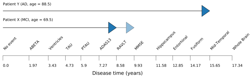
Figure 1: AD timeline inferred by EB-HMM. The order of events on the horizontal axis is given by $\overline{S}$, and the time between events is calculated from $\overline{Q}$. Baseline stage (solid arrow) and predicted next stage (shaded arrow) estimated by EB-HMM for two example patients are shown, chosen from the MCI and AD sub-groups.

3.2 Comparative model performance

We train EB-HMM and a continuous-time hidden Markov model (CT-HMM) to infer individual-level stage sequences and hence compare predictive accuracy on a common task. Specifically, we use baseline stage as a predictor of conversion from CN to MCI, or MCI to AD, over a period of two years. Here predicted converters are defined as people with a stage greater than a threshold stage, which is iterated across all possible stages. We calculate the area under receiver operating characteristic curve (AU-ROC), and perform 5-fold cross-validation. Table LABEL:tab:comp shows that EB-HMM performs substantially better than CT-HMM in both the full (including individuals with missing data) and subset data (only individuals with complete data).

tab:comp 2.2exModel AU-ROC EB-HMM (full) $\mathbf{0.804\pm 0.07}$ EB-HMM (subset) $0.737\pm 0.09$ CT-HMM (subset) $0.579\pm 0.12$

Table 1: EB-HMM and CT-HMM performance for the task of predicting conversion, using either the full or subset data.

3.3 Performance with missing data

Finally, we demonstrate the ability of EB-HMM to handle missing data. We randomly discard $25\%$, $50\%$, and $75\%$ of the feature data from each individual in the subset data and re-train EB-HMM. As in sec:comp, we use prediction of conversion as the task and 5-fold cross-validation to obtain out-of-sample estimates of the AU-ROC. Table LABEL:tab:miss shows that EB-HMM maintains consistent performance up to $50\%$ missing data, and drops off only moderately for $75\%$.

tab:miss 2.2ex$\%$ missing AU-ROC $25\%$ $0.722\pm 0.09$ $50\%$ $0.719\pm 0.13$ $75\%$ $0.669\pm 0.15$

Table 2: EB-HMM performance for the task of predicting conversion with missing data.

4 Discussion

Future work on EB-HMM will be focused on relaxing its assumptions, namely $i)$ monotonic biomarker change; $ii)$ a consistent event sequence across the whole sample; and $iii)$ Markov (memoryless) stage transitions. Assumption $i)$ is both a limitation and a strength: it allows us to simplify our model at the expense of requiring monotonic biomarker change; as shown here, for truly monotonic clinical, imaging and biofluid markers it only provides benefits. However for non-monotonic markers – such as heart rate – either the model or data would need to be adapted. Assumptions $ii)$ and $iii)$ could be relaxed by combining our EB-HMM framework with (for example) subtype modelling Young et al. (2018) and semi-Markov modelling Alaa and van der Schaar (2018), respectively. In particular, EB-HMM can be directly integrated into the subtyping and staging framework proposed by Young et al. (2018), which would allow us to capture the well-reported heterogeneity in AD and produce timelines such as Figure LABEL:fig:timeline for separate subtypes. This opens up the prospect of developing a probabilistic model that can infer interpretable longitudinal subtypes from limited datasets. We thank all the ADNI study participants.

Appendix A Appendix

A.1 Event-Based Hidden Markov Model

We can write the EB-HMM joint distribution over all variables in a hierarchical Bayesian framework:

$$\begin{split}P(S,\theta,k,Y)=P(S)\cdot P(\theta|S)\\ \cdot P(k|\theta,S)\cdot P(Y|k,\theta,S).\end{split}$$ (6)

Here $S$ is the hidden sequence of events, $\theta$ are the distribution parameters generating the data, $k$ is the hidden disease state, and $Y$ are the observed data. Graphical models of CT-HMM and EB-HMM are shown in Figure LABEL:fig:graphs. Note that we have assumed conditional independence of $S$ from $k$; that is, the complete set of disease progression states is independent of the time of observation.

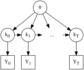
fig:graphs [CT-HMM]  [EB-HMM]

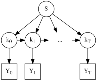
Figure 2: Graphical models for (a) CT-HMM and (b) EB-HMM. Hidden variables are denoted by circles, observations by squares. $S$: sequence of events; $\theta$: distribution parameters; $k$: disease state; $Y$: observed data; $T$: observed time.

Assuming independence between observed features $i=1,...,I$, if a patient $j=1,...,J$ is at latent state $k_{j,t}=0,...,N$ at time $t=1,...,T_{j}$ in the progression model, the likelihood of their data $Y_{j,t}$ is given by:

$$\begin{split}P(Y_{j,t}|k_{j,t},\theta,S)=\prod_{i=1}^{I}P(Y_{i,j,t}|k_{j,t},\theta_{i},S).\end{split}$$ (7)

Here $\theta_{i}$ are the distribution parameters for feature $i$, defined by a hidden sequence of events $S=(s(1),...,S(N))$. Following Fonteijn et al. (2012), we enforce the monotonicity hypothesis by requiring $S$ to be ordered, meaning individuals at stage $k_{j,t}$ cannot revert back to an earlier stage. This assumption is necessary to allow snapshots from different individuals to inform on the full event ordering. Next, we assume a Markov jump process between discrete time-points:

$$\begin{split}P(Y_{j}|k_{j},\theta,S)=P(k_{j,t=0})\prod_{t=1}^{T_{j}}P(k_{j,t}|k_{j,t-1})\\ \prod_{t=0}^{T_{j}}\prod_{i=1}^{I}P(Y_{i,j,t}|k_{j,t},\theta_{i},S).\end{split}$$ (8)

To obtain an event-based model, we now define prior values for the distribution parameters $\theta$ for each state $k$ in sequence $S$. Following Fonteijn et al. (2012) we choose a two-component Gaussian mixture model to describe the data likelihood:

$$\begin{split}\prod_{i=1}^{I}P(Y_{i,j,t}|k_{j,t},\theta_{i},S)=\prod_{i=1}^{k_{j,t}}P(Y_{i,j,t}|k_{j,t},\theta^{p}_{i},S)\\ \prod_{i=k_{j,t}+1}^{I}P(Y_{i,j,t}|k_{j,t},\theta^{c}_{i},S)\end{split}$$ (9)

Here $\theta^{p}_{i}=[\mu^{p}_{i},\sigma^{p}_{i},w^{p}_{i}]$ and $\theta^{c}_{i}=[\mu^{c}_{i},\sigma^{c}_{i},w^{c}_{i}]$ are the mean, $\mu$, standard deviation, $\sigma$, and mixture weights, $w$, for the patient and control distributions, respectively. Note that these distributions are fit prior to inference, which requires our data to contain labels for patients and controls; however, once $\theta^{p}_{i}$ and $\theta^{c}_{i}$ have been fit, the model can infer $S$ without any labels. One of the strengths of the mixture model approach is that when feature data are missing, the two probabilities on the RHS of Equation 9 can simply be set equal.

To obtain the total data likelihood, we marginalize over the hidden state $k$ and assume independence between measurements from different individuals $j$ (dropping indices $j,t$ in the sum for notational simplicity):

$$\begin{split}P(Y|\theta,S)=\prod_{j=1}^{J}\left[\sum_{k=0}^{N}P(k_{j,t=0})\prod_{t=1}^{T_{j}}P(k_{j,t}|k_{j,t-1})\right.\\ \left.\prod_{t=0}^{T_{j}}\prod_{i=1}^{k_{j,t}}P(Y_{i,j,t}|k_{j,t},\theta^{p}_{i},S)\right.\\ \left.\prod_{i=k_{j,t}+1}^{I}P(Y_{i,j,t}|k_{j,t},\theta^{c}_{i},S)\right].\end{split}$$ (10)

We can now use Bayes’ theorem to obtain the posterior distribution over $S$. We note that Equation 10 is the time generalisation of the model presented by (Fonteijn et al., 2012), and for $T_{j}=1$ it reduces to that model. We further note that Equation 8 looks like a CT-HMM  Ghahramani (2001). The mathematical innovation of our work is to reformulate the EBM in a CT-HMM framework. To our knowledge this is the first such model of its type.

A.2 Inference scheme

We use a nested inference scheme based on iteratively optimising the sequence $S$, and fitting the initial probability $\pi_{a}$ and transition matrix $Q_{a,b}$, to find a local maximum via a nested application of the Expectation-Maximisation (EM) algorithm. At the first EM step, $S$ is optimised for the current values of the initial probability $\pi^{\prime}_{a}$ and transition matrix $Q^{\prime}_{a,b}$, by permuting the position of every event separately while keeping the others fixed. At the second step, $\pi_{a}$ and $Q_{a,b}$ are fitted for the current sequence $S^{\prime}$ using the standard forward-backward algorithm Rabiner (1989). Here we apply only a single pass, as iterative updating of $\pi_{a}$ and $Q_{a,b}$ while keeping $S$ (and hence $\theta_{i}$) fixed effectively turns the optimisation problem into repeated scaling of the posterior, which causes over-fitting of $\pi_{a}$ and $Q_{a,b}$.

Input : $Y$

Output : $S$, $\pi$, $Q$

Initialise $S$;

while not $S$ converged do

       // E-step of sequence optimisation

       while not every event permuted do

             Initialise $\pi$, $Q$;

             // E-step of transition and initial probability optimisation

             Compute $\gamma_{a,t}=P(k_{t}=a|Y,S=S^{\prime};\pi,Q)$;

             Compute $\xi_{a,b,t}=P(k_{t}=a,k_{t+1}=b|Y,S=S^{\prime};Q)$;

             // M-step of transition and initial probability optimisation

             Update $\pi_{a}\leftarrow\gamma_{a,0}$;

             Update $Q_{a,b}\leftarrow\dfrac{\sum_{t=1}\xi_{a,b,t}}{\sum_{t=1}\gamma_{a,t-1}}$;

             Compute $\mathcal{L}(S)=\mathrm{log}P(Y|S;\pi^{\prime},Q^{\prime})$;

            

       end while

      // M-step of sequence optimisation

       Update $S\leftarrow\mathrm{arg\,max}_{S}\mathcal{L}(S)$;

      

end while

Algorithm 1 EB-HMM inference

A.3 Alzheimer’s disease data

We use data from the ADNI study, a longitudinal multi-centre observational study of AD Mueller et al. (2005). We select 468 participants (119 CN: cognitively normal; 297 MCI: mild cognitive impairment; 29 AD: manifest AD; 23 NA: not available), and three time-points per participant (baseline and follow-ups at 12 and 24 months). Individuals were allowed to have missing data at any time-point. Note that we use a subset of 368 individuals with no missing data in Sections 3.2 and 3.3. We train on a mix of 12 clinical, imaging and biofluid features. The clinical data are three cognitive markers: ADAS-13, Rey Auditory Verbal Learning Test (RAVLT) and Mini-Mental State Examination (MMSE). The imaging data are T1-weighted 3T structural magnetic resonance imaging (MRI) scans, post-processed to produce regional volumes using the GIF software tool Cardoso et al. (2015). We select a subset of sub-cortical and cortical regional volumes with reported sensitivity to AD pathology, namely the hippocampus, ventricles, entorhinal, mid-temporal, and fusiform, and the whole brain Frisoni et al. (2010). The biofluid data are three cerebrospinal fluid markers: amyloid-$\beta_{1-42}$ (ABETA), phosphorylated tau (PTAU) and total tau (TAU). The TADPOLE challenge dataset Marinescu et al. (2020) used in this paper is freely available upon registering with an ADNI account.

A.4 Model training

We compare EB-HMM and CT-HMM algorithms. To ensure fair comparison, we impose a constraint on both models by placing a 2nd order forward-backward prior on the transition matrix. For EB-HMM, we fit Gaussian mixture models to the distributions of AD (patients) and CN (controls) sub-groups prior to running Algorithm 1. For CT-HMM, we apply the standard forward-backward algorithm and iterate the likelihood to convergence within $10^{-2}$ of the total model likelihood. We initialise the CT-HMM prior mean and covariance matrices from the training data, using standard $k$-means and the feature covariance, respectively. EB-HMM is implemented and parallelised in Python; open-source code will be provided upon full journal publication at the author’s repository: https://github.com/pawij/tebm.

References

- Alaa and van der Schaar (2018) A. M. Alaa and M. van der Schaar. A hidden absorbing semi-markov model for informatively censored temporal data: Learning and inference. Journal of Machine Learning Research, 70:60–69, 2018. http://dx.doi.org/10.5555/3305381.3305388.
- Cardoso et al. (2015) M. J. Cardoso, M. Modat, R. Wolz, et al. Geodesic information flows: Spatially-variant graphs and their application to segmentation and fusion. IEEE Transactions on Medical Imaging, 34:1976–1988, 2015. https://doi.org/10.1109/TMI.2015.2418298.
- Cummings et al. (2019) J. Cummings, G. Lee, A. Ritter, M. Sabbagh, and K. Zhong. Alzheimer’s disease drug development pipeline: 2019. Alzheimer’s Dement, 5:272–293, 2019. http://dx.doi.org/10.1016/j.trci.2019.05.008.
- Dorsey et al. (2015) E. R. Dorsey, C. Venuto, V. Venkataraman, D. A. Harris, and K. Kieburtz. Novel methods and technologies for 21st-century clinical trials. JAMA Neurol, 72(5):582–588, 2015. http://dx.doi.org/10.1001/jamaneurol.2014.4524.
- Dubois et al. (2016) B. Dubois, H. Hampel, H. H. Feldman, et al. Preclinical alzheimer’s disease: definition, natural history, and diagnostic criteria. Alzheimers Dement, 12(3):292–323, 2016. http://dx.doi.org/10.1016/j.jalz.2016.02.002.
- Fonteijn et al. (2012) H. M. Fonteijn, M. Modat, M. J. Clarkson, and colleagues. An event-based model for disease progression and its application in familial alzheimer’s disease and huntington’s disease. NeuroImage, 60:1880–1889, 2012. https://doi.org/10.1016/j.neuroimage.2012.01.062.
- Frisoni et al. (2010) G. B. Frisoni, N. C. Fox, C. R. Jack, P. Scheltens, and P. M. Thompson. The clinical use of structural mri in alzheimer disease. Nat Rev Neurol, 6(2):67–77, 2010. http://dx.doi.org/10.1038/nrneurol.2009.215.
- Ghahramani (2001) Z. Ghahramani. An introduction to hidden markov models and bayesian networks. Journal of Pattern Recognition and Artificial Intelligence, 15:9–42, 2001.
- Huang and Alexander (2012) J. Huang and D. C. Alexander. Probabilistic event cascades for alzheimer’s disease. Advances in Neural Information Processing Systems, 25, 2012.
- Jack and Holtzman (2013) C. R. Jack and D. M. Holtzman. Biomarker modeling of alzheimer’s disease. Neuron, 80(6):1347–1358, 2013. http://dx.doi.org/10.1016/j.neuron.2013.12.003.
- Marinescu et al. (2020) R. V. Marinescu, N. P. Oxtoby, A. L. Young, et al. The alzheimer’s disease prediction of longitudinal evolution (tadpole) challenge: Results after 1 year follow-up. arXiv, 2020. URL https://arxiv.org/abs/2002.03419.
- Masters et al. (2015) C. L. Masters, R. Bateman, K. Blennow, C. C. Rowe, R. A. Sperling, and J. L. Cummings. Alzheimer’s disease. Nat Rev Dis Primers, 1(15056), 2015. http://dx.doi.org/10.1038/nrdp.2015.5.
- Mueller et al. (2005) S. G. Mueller, M. W. Weiner, L. J. Thal, et al. The alzheimer’s disease neuroimaging initiative. Neuroimaging Clin N Am, 15:869–877, 2005. https://doi.org/10.1016/j.nic.2005.09.008.
- Oxtoby and Alexander (2017) N. P. Oxtoby and D. C. Alexander. Imaging plus x: multimodal models of neurodegenerative disease. Curr Opin Neurol, 30(4):371–379, 2017. http://dx.doi.org/10.1097/WCO.0000000000000460.
- Oxtoby et al. (2018) N. P. Oxtoby, A. L. Young, D. M. Cash, and colleagues. Data-driven models of dominantly-inherited alzheimer’s disease progression. Brain, 141:1529–1544, 2018. https://doi.org/10.1093/brain/awy050.
- Rabiner (1989) L.R. Rabiner. A tutorial on hidden markov models and selected applications in speech recognition. IEEE, 77:257–286, 1989. https://doi.org/10.1109/5.18626.
- Wang et al. (2014) X. Wang, D. Sontag, and F. Wang. Unsupervised learning of disease progression models. Proceedings of the 20th ACM SIGKDD International Conference on Knowledge Discovery and Data Mining, 2014. http://dx.doi.org/10.1145/2623330.2623754.
- Young et al. (2014) A. L. Young, N. P. Oxtoby, P. Daga, and colleagues. A data-driven model of biomarker changes in sporadic alzheimer’s disease. Brain, 137:2564–2577, 2014. https://doi.org/10.1093/brain/awu176.
- Young et al. (2018) A. L. Young, R. V. Marinescu, N. P. Oxtoby, and colleagues. Uncovering the heterogeneity and temporal complexity of neurodegenerative diseases with subtype and stage inference. Nature Communications, 9, 2018. https://doi.org/10.1038/s41467-018-05892-0.