Chess2vec: Learning Vector Representations for Chess

Abstract

We conduct the first study of its kind to generate and evaluate vector representations for chess pieces. In particular, we uncover the latent structure of chess pieces and moves, as well as predict chess moves from chess positions. We share preliminary results which anticipate our ongoing work on a neural network architecture that learns these embeddings directly from supervised feedback.

The fundamental challenge for machine learning based chess programs is to learn the mapping between chess positions and optimal moves [5, 3, 7]. A chess position is a description of where pieces are located on the chessboard. In learning, chess positions are typically represented as bitboard representations [1].

A bitboard is a $8\times 8$ binary matrix, same dimensions as the chessboard, and each bitboard is associated with a particular piece type (e.g. pawn) and player color (e.g. black). On the bitboard, an entry is $1$ if a piece associated with the bitboard’s type and color exists on the corresponding chessboard location, and $0$ otherwise. Each chess position is represented using $12$ bitboards, where each bitboard corresponds to a different piece type (i.e. king, queen, rook, bishop, knight, or pawn) and player color (i.e. white or black). More formally, each chess position is represented as a $8\times 8\times 12$ binary tensor.

The bitboard representation can alternatively be specified by assigning a $12$-dimensional binary vector to each piece type and color. Under this interpretation, given a chess position, each of the $64$ chessboard locations is assigned a $12$-dimensional vector based on the occupying piece. If the location has no piece, it is assigned the zero vector, and if it has a piece, it is assigned the sparse indicator vector corresponding to the piece type and color. Note that, with this representation, all black pawns would be represented using the same vector.

In this paper, our goal is to explore new $d$-dimensional vector representations for chess pieces to serve as alternatives to the $12$-dimensional binary bitboard representation.

1 Latent structure of pieces and moves

In this section, we analyze the latent structure of chess pieces and moves using principal components analysis. We conduct the analysis on two different datasets: one which contains legal moves and another which contains expert moves. Aside from gaining qualitative insights about chess, we also obtain our first vector representations.

1.1 Principal component analysis (PCA)

PCA is a method for linearly transforming data into a lower-dimensional representation [4]. In particular, let data be represented as the matrix $X\in\mathbb{R}^{n\times p}$ whose columns have zero mean and unit variance. Each row of $X$ can be interpreted as a data point with $p$ features. Then, PCA computes the transformation matrix $C^{\star}\in\mathbb{R}^{p\times d}$ by solving the optimization problem

$$\begin{aligned} &\underset{C}{\text{minimize}}&&\left\|X-XCC^{T}\right\|_{F}^{2}\\ &\text{subject to}&&C^{T}C=I\end{aligned}.$$ (1)

Intuitively, $C^{\star}$ linearly transforms the data from a $p$-dimensional space to a $d$-dimensional space in such a way that the inverse transformation (i.e. reconstruction) minimizes the Frobenius norm. The mapping of $X$ into the $d$-dimensional space is given by $W=XC^{\star}$. The importance of minimizing reconstruction error will be clear when we quantitatively evaluate the embeddings obtained via PCA.

In order to apply PCA to chess, we need an appropriate way to represent chess data as $X\in\mathbb{R}^{n\times p}$. Ideally, we would like pieces with similar movement patterns to have similar low-dimensional representations, so we represent each piece by its move counts. In its simplest form, a chess move is specified via a source board location that a piece is picked from and a target board location that the piece is moved into. This formulation allows us to avoid specifying the type of the moving piece or whether the target location already contained another piece. There are $64$ board locations, thus all move counts can be represented via a $4096$-dimensional vector, and since there are $6$ piece types, we let $X\in\mathbb{R}^{6\times 4096}$.

1.2 Stockfish moves

We generate the count matrix $X\in\mathbb{R}^{n\times p}$ by pitting two Stockfish [2] engines against each other and logging their moves. In order to investigate how pieces of the same type are similar to or different from each other, we let each row of $X$ correspond to a piece rather than a piece type. Hence, we set $n$ to $16$, which is the number of white pieces.

We let the engines play against each other for $4{,}000{,}000$ turns, resulting in $23{,}096$ games with an average length of $173$ turns. White player wins $45\%$ of the time, black player wins $10\%$ of the time, and a draw occurs $45\%$ of the time. We observe a high percentage of draws because repeating the same move three times causes a draw, and the black player frequently uses that strategy. We only log moves by the white player from the games which the white player won, yielding a total of $881{,}779$ moves, which we use to construct the $X\in\mathbb{R}^{16\times 4096}$ matrix. We then normalize each row by its total counts, scale the columns to have zero mean and unit variance, and apply PCA.

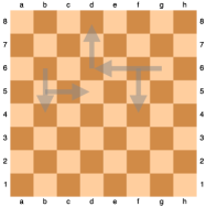
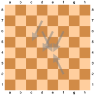
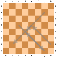
Figure 1: The top five moves associated with the Stockfish loading vectors.

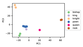
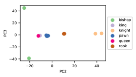
Figure 2: Principal component scores of chess pieces (Stockfish moves). Left: the first principal component versus the second. Right: the second principal component versus the third.

We visualize the first three components in Figure 2. Each loading vector can be interpreted as a fundamental building block of expert chess moves, and the principal component scores depict how each piece can be described in terms of these building blocks. The first five principal components explain $81.0\%$ of the variance in the movement data, at which point adding more principal components does not increase the explained variance by much. This is because, as seen in Figure 2, pieces of same type have similar principal component scores, and they share the same loading vectors to construct their movement patterns. This is surprising, since PCA has no explicit information that these pieces belong to the same type, and despite their similarities, individual pieces such as pawns do have their own unique movement patterns within the $4096$-dimensional movement space.

In figure 1, we display the highest scored moves associated with the loading vectors. The third dimension is the first dimension in which pieces of the same type, namely bishops, are not clustered together with respect to their component scores. In fact, the bishop which moves among black squares has a high component score, and the bishop which moves among white squares has a low component score.

These decompositions are helpful in uncovering fundamental movement patterns and understanding the relationship between pieces with respect to these patterns. To the best of our knowledge, this is the first attempt to use machine learning to conduct such an analysis. In the process, we have also obtained our first $d$-dimensional vector representations, namely $W=XC^{\star}$.

2 Position-dependent piece vectors

In this section, we attempt to improve upon the vector representations we have obtained so far. In particular, one potential issue is that the piece vectors we constructed are constant with respect to chess positions. For example, the vector representation of a pawn does not vary based on the remaining pieces on the board. We propose a hash-based method to address this issue. We also conduct our first quantitative evaluation.

2.1 Zobrist hashing

Zobrist hashing [8] is a method for constructing a universal hash function that was originally developed for abstract board games. It is typically used to build transposition tables which prevent game agents from analyzing the same position more than once.

A natural way to generate position-dependent piece vectors is to modify the construction of the count matrix $X\in\mathbb{R}^{n\times p}$. Previously, each row of $X$ corresponded to a piece or piece type. This time, we expand the rows to correspond to the Cartesian product of pieces and hash buckets. The hash buckets partition the space of all chess positions via Zobrist hashing. Thus, instead of generating a unique vector representation for each piece, we generate it for each piece given a hash bucket, where each bucket represents a random collection of chess positions. In our experiments, we let the number of hash buckets go up to $32{,}768$. Since there are $16$ pieces, this yields the sparse count matrix $X\in\mathbb{R}^{524{,}288\times 4096}$.

2.2 Non-negative matrix factorization (NMF)

In addition to expanding the count matrix, we also switch our matrix factorization method from PCA to NMF [6]. NMF is specified by the optimization problem

$$\begin{aligned} &\underset{W,H}{\text{minimize}}&&\left\|X-WH\right\|_{F}^{2}\\ &\text{subject to}&&W\geq 0,H\geq 0\end{aligned}.$$ (2)

In the NMF objective (2), $W\in\mathbb{R}^{n\times d}$ encodes the $d$-dimensional vector representations and $H\in\mathbb{R}^{d\times p}$ encodes the $p$-dimensional basis vectors. The corresponding matrices in the PCA objective (1) are $W\simeq XC$ and $H\simeq C^{T}$, where $\simeq$ simply denotes a semantic (but not a numeric) similarity.

We switch from PCA to NMF for a couple of reasons. First, even though both PCA and NMF attempt to minimize the reconstruction error, the positivity constraints of NMF are more flexible than the orthonormality constraints of PCA. In fact, NMF yields lower reconstruction error than PCA, and as we shall see below, reconstruction error plays an important role in predicting chess moves. Second, NMF yields a different set of vectors than PCA which are also worth investigating.

We demonstrate how matrix reconstruction can be used to predict chess moves from chess positions. As discussed, each row of $W\in\mathbb{R}^{n\times d}$ encodes a $d$-dimensional vector representation, denoted as $w_{i,j}^{T}\in\mathbb{R}^{1\times d}$, that is associated with a white piece $i\in\left\{1,\ldots,16\right\}$ and a hash bucket $j$. Each hash bucket $j$ corresponds to a random collection of chess positions. Let $w_{0,.}$ be the vector representation for the special piece $0$ that is always assigned to the zero vector. Let $s\in\mathcal{S}$ represent a chess position, which is a description of the locations of all the pieces on a chess board. Let $f_{l}:\mathcal{S}\to\{0,...,16\}$ be a function that maps a chess position to one of the $17$ pieces that can be located on board location $l\in\{1,...,64\}$, where $f_{l}\left(s\right)=i$ if board location $l$ contains a white piece $i$, and $f_{l}\left(s\right)=0$ if $l$ is empty or contains a black piece. Let $h:\mathcal{S}\to\mathcal{J}$ be the Zobrist hash function that maps a chess position to a hash bucket. Then, given a chess position $s$, $y\left(s\right)=\sum_{j=1}^{64}H^{T}w_{f_{j}\left(s\right),h\left(s\right)}$ is the $4096$-dimensional prediction vector, and $\operatorname*{arg\,max}_{{}_{i}}y\left(s\right)_{i}$ is the index of the predicted move.

The intuition behind this prediction is as follows. Each row of $X$, denoted as $x_{i,j}^{T}\in\mathbb{R}^{1\times 4096}$, represents the number of times a white piece $i$ has been associated with a particular move for chess positions in $\mathcal{S}_{j}=\left\{s\in\mathcal{S}\mid h\left(s\right)=j\right\}$. Since equation 2 minimizes reconstruction error, given a chess position $s$, $H^{T}w_{f_{j}\left(s\right),h\left(s\right)}\approx x_{f_{j}\left(s\right),h\left(s\right)}$. Thus, $y\left(s\right)\approx\sum_{j=1}^{64}x_{f_{j}\left(s\right),h\left(s\right)}$ approximates the number of times a move has been selected for all the chess positions that are hashed into bucket $j$.

2.3 Quantitative evaluation

In this subsection, we evaluate the accuracy of making move predictions using matrix reconstruction and position-dependent piece vectors. We split the Stockfish data, which consists of $881{,}779$ moves, into $80\%$ train and $20\%$ test. We use the train data to generate the count matrix $X\in\mathbb{R}^{524{,}288\times 4096}$, apply NMF, and obtain $W_{\text{train}}$ and $H_{\text{train}}$. We then iterate over each chess position $s$ in test data, replace their bitboard vectors with the relevant rows from $W_{\text{train}}$, and compute $y\left(s\right)$.

Figure 3: Test multiclass accuracy of matrix reconstruction with position-dependent piece vectors.

In figure 3, we display the multiclass accuracy on held-out test data. As we increase the number of hash buckets, the held-out accuracy improves. With $32768$ hash buckets, this method predicts $8.8\%$ of Stockfish moves correctly, on a task with $4096$ classes.

References

- [1] Wikipedia contributors. Bitboard — Wikipedia, The Free Encyclopedia. https://en.wikipedia.org/w/index.php?title=Bitboard&oldid=841136708, 2018.
- [2] Wikipedia contributors. Stockfish (chess) — Wikipedia, The Free Encyclopedia. https://en.wikipedia.org/w/index.php?title=Stockfish_(chess)&oldid=855275247, 2018.
- [3] Omid E. David, Nathan S. Netanyahu, and Lior Wolf. DeepChess: End-to-end deep neural network for automatic learning in chess. In ICANN, 2016.
- [4] Gareth James, Daniela Witten, Trevor Hastie, and Robert Tibshirani. An Introduction to Statistical Learning. 2013.
- [5] Matthew Lai. Giraffe: Using deep reinforcement learning to learn to play chess. arXiv, 2015.
- [6] Daniel D. Lee and H. Sebastian Seung. Learning the parts of objects by non-negative matrix factorization. Nature, 1999.
- [7] David Silver, Thomas Hubert, Julian Schrittwieser, Ioannis Antonoglou, Matthew Lai, Arthur Guez, Marc Lanctot, Laurent Sifre, Dharshan Kumaran, Thore Graepel, Timothy Lillicrap, Karen Simonyan, and Demis Hassabis. Mastering Chess and Shogi by Self-Play with a General Reinforcement Learning Algorithm. arXiv, 2017.
- [8] Albert L Zobrist. A new hashing method with application for game playing. ICCA Journal, 13(2):69–73, 1970.