Out of Control: Reducing Probabilistic Models by Control-State Elimination

Abstract

State-of-the-art probabilistic model checkers perform verification on explicit-state Markov models defined in a high-level programming formalism like the PRISM modeling language. Typically, the low-level models resulting from such program-like specifications exhibit lots of structure such as repeating subpatterns. Established techniques like probabilistic bisimulation minimization are able to exploit these structures; however, they operate directly on the explicit-state model. On the other hand, methods for reducing structured state spaces by reasoning about the high-level program have not been investigated that much. In this paper, we present a new, simple, and fully automatic program-level technique to reduce the underlying Markov model. Our approach aims at computing the summary behavior of adjacent locations in the program’s control-flow graph, thereby obtaining a program with fewer “control states”. This reduction is immediately reflected in the program’s operational semantics, enabling more efficient model checking. A key insight is that in principle, each (combination of) program variable(s) with finite domain can play the role of the program counter that defines the flow structure. Unlike most other reduction techniques, our approach is property-directed and naturally supports unspecified model parameters. Experiments demonstrate that our simple method yields state-space reductions of up to 80% on practically relevant benchmarks.

1 Introduction

Modelling Markov models.

Probabilistic model checking is a fully automated technique to rigorously prove correctness of a system model with randomness against a formal specification. Its key algorithmic component is computing reachability probabilities on stochastic processes such as (discrete- or continuous-time) Markov chains and Markov Decision Processes. These stochastic processes are typically described in some high-level modelling language. State-of-the-art tools like PRISM [34], storm [27] and mcsta [25] support input models specified in e.g., the PRISM modeling language, PPDDL [42], a probabilistic extension of the planning domain definition language [23], the process algebraic language MoDeST [9], the jani model exchange format [11], or the probabilistic guarded command language pGCL [35]. The recent tool from [22] even supports verification of probabilistic models written in Java.

Model construction.

Prior to computing reachability probabilities, existing model checkers explore all the program’s reachable variable valuations and encode them into the state space of the operational Markov model. Termination is guaranteed as variables are restricted to finite domains. This paper proposes a simple reduction technique for this model construction phase that avoids unfolding the full model prior to the actual analysis, thereby mitigating the state explosion problem. The basic idea is to unfold variables one-by-one—rather than all at once as in the standard pipeline—and apply analysis steps after each unfolding. We detail this control-state reduction technique for probabilistic control-flow graphs and illustrate its application to the PRISM modelling language. Its principle is however quite generic and is applicable to the aforementioned modelling formalisms. Our technique is thus to be seen as a model simplification front-end for general purpose probabilistic model checkers.

Approach.

Technically our approach works as follows. The principle is to unfold a (set of) variable(s) into the control state space, a technique inspired by static program analyses such as abstract interpretation [29]. The selection of which variables to unfold is property-driven, i.e., depending on the reachability or reward property to be checked. We define the unfolding on probabilistic control-flow programs [20] (PCFPs, for short) and simplify them using a technique that generalizes state elimination in (parametric) Markov chains [14]. Our elimination technique heavily relies on classical weakest precondition reasoning [17]. This enables the elimination of several states at once from the underlying “low-level” Markov model while preserving exact reachability probabilities or expected rewards. Figure 1 provides a visual intuition on the resulting model compression.

The choice of the variables and locations for unfolding and elimination, resp., is driven by heuristics. In a nutshell, our unfolding heuristics prefers the variables that lead to a high number of control-flow locations without self-loops. These loop-free locations are then removed by the elimination heuristics which gives preference to locations whose removal does not blow up the transition matrix of the underlying model. Unfolding and elimination steps are performed in an alternating fashion, but only until the PCFP size reaches a certain threshold. After this, the reduction phase is complete and the transformed PCFP can be fed into a standard probabilistic model checker.

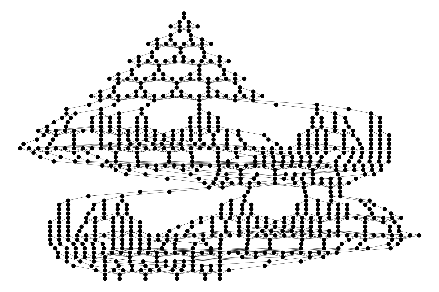
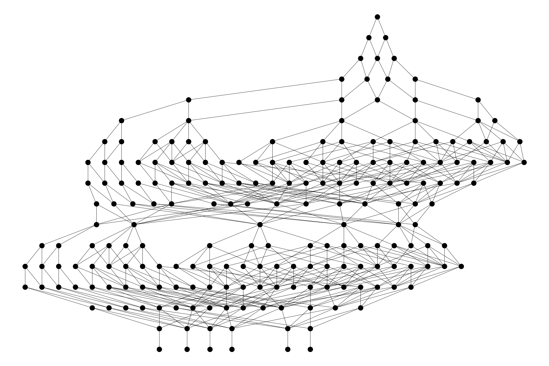
Figure 1: Left: Visualization of the original nand model from [36] (930 states, parameters 5/1). Transitions go from top to bottom. Right: The same model after our reduction ($207$ states). A single “program counter variable” taking at most 5 different values was unfolded and a total of three locations were eliminated thereafter. Note that the overall structure is preserved but several local substructures such as the pyramidal shape at the top are compressed significantly. This behavior is typical for our approach.

Contributions.

In summary, the main contributions of this paper are:

• A simple, widely applicable reduction technique that considers each program variable with finite domain as a “program counter” and selects suitable variables for unfolding into the control state space one-by-one.

• A sound rule to eliminate control-flow locations in PCFPs in order to shrink the state space of the underlying Markov model while preserving exact reachability probabilities or expected rewards.

• Elimination in PCFPs—in contrast to Markov chains—is shown to have an exponential worst-case complexity.

• An implementation in the probabilistic model checker storm demonstrating the potential to significantly compress practically relevant benchmarks.

Related work.

The state explosion problem has been given top priority in both classical and probabilistic model checking. Techniques similar to ours have been known for quite some time in the non-probabilistic setting [19, 33]. Regarding probabilistic model checking, reduction methods on the state-space level include symbolic model checking using MTBDDs [1], SMT/SAT techniques [41, 7], bisimulation minimization [31, 39, 28], Kronecker representations [10, 1] and partial order reduction [4, 13]. Language-based reductions include symmetry reduction [18], bisimulation reduction using SMT on PRISM modules [16], as well as abstraction-refinement techniques [32, 24, 40]. Our reductions on PCFPs are inspired by state elimination [14]. Similar kinds of reductions on probabilistic workflow nets have been considered in [21]. Despite all these efforts, it is somewhat surprising that simple probabilistic control-flow reductions as proposed in this paper have not been investigated that much. A notable exception is the recent work by Dubslaff et al. that applies existing static analyses to control-flow-rich PCFPs [20]. In contrast to our method, their technique yields bisimilar models and exploits a different kind of structure.

Organization of the paper.

Section 2 starts off by illustrating the central aspects of our approach by example. Section 3 defines PCFPs and their semantics in terms of MDPs. Section 4 formalizes the reductions, proves their correctness and analyzes the complexity. Our implementation in storm is discussed in Section 5. We present our experimental evaluation in Section 6 and conclude in Section 7.

2 A Bird’s Eye View

This section introduces a running example to illustrate our approach. Consider a game of chance where a gambler starts with an initial budget of $\mathtt{x=N/2}$ tokens. The game is played in rounds, each of which either increases or decreases the budget. The game is lost once the budget has dropped to zero and won once it exceeds $\mathtt{N}$ tokens. In each round, a fair coin is tossed: If the outcome is tails, then the gambler loses one token and proceeds to the next round; on the other hand, if heads occurs, then the coin is flipped again. If tails is observed in the second coin flip, then the gambler also loses one token; however, if the outcome is again heads then the gambler receives two tokens.

In order to answer questions such as “Is this game fair?” (for a fixed $\mathtt{N}$), probabilistic model checking can be applied. To this end, we model the game as the PRISM program in Figure 2. We briefly explain its central components: The first two lines of the module block are variable declarations. Variable $\mathtt{x}$ is an integer with bounded domain and $\mathtt{f}$ is a Boolean. The idea of $\mathtt{x}$ and $\mathtt{f}$ is to represent the current budget and whether the coin has to be flipped a second time, respectively. The next three lines that each begin with [] define commands which are interpreted as follows: If the guard on the left-hand side of the arrow -> is satisfied, then one of the updates on the right side is executed with its corresponding probability. For instance, in the first command, $\mathtt{x}$ is decremented by one (and $\mathtt{f}$ is left unchanged) with probability $1/2$. Otherwise $\mathtt{f}$ is set to true. The order in which the commands occur in the program text is irrelevant. If there is more than one command enabled for a specific valuation of the variables, then one of them is chosen non-deterministically. Our example is, however, deterministic in this regard since the three guards are mutually exclusive.

dtmc const int N; module coingame x : [0..N+1] init N/2; f : bool init false; [] 0¡x & x¡N !f -¿ 1/2: (x’=x-1) + 1/2: (f’=true); [] 0¡x x¡N f -¿ 1/2: (x’=x-1) (f’=false) + 1/2: (x’=x+2) (f’=false); [] x=0 — x¿=N -¿ 1: (f’=false); endmodule

Figure 2: The coin game as a PRISM program. Variable $\mathtt{x}$ stands for the current budget.

Probabilistic model checkers like PRISM and storm expand the above program as a Markov chain with approximately $2\mathtt{N}$ states. This is depicted for $\mathtt{N}=6$ at the top of Figure 3. Given that we are only interested in the winning probability (i.e., to reach one of the two rightmost states), this Markov chain is equivalent to the smaller one on the bottom of Figure 3. Indeed, eliminating each dashed state in the lower row individually yields that the overall probability per round to go one step to the left is $3/4$ and $1/4$ to go two steps to the right. On the program level, this simplification could have been achieved by summarizing the first two commands to [] 0¡x & x¡N -¿ 3/4: (x’=x-1) + 1/4: (x’=x+2);

so that variable $\mathtt{f}$ is effectively removed from the program.

Figure 3: Top: The Markov chain of the original coin game for $\mathtt{N}=6$. All transition probabilities (except on the self-loops) are $1/2$. Bottom: The Markov chain of the simplified model.

Obtaining such simplifications in an automated manner is the main purpose of this paper. In summary, our proposed solution works as follows:

1. First, we view the input program as a probabilistic control flow program (PCFP), which can be seen as a generalization of PRISM programs from a single to multiple control-flow locations (Figure 4, left). A PRISM program (with a single module) is a PCFP with a unique control location. Imperative programs such as pGCL programs [35] can be regarded as PCFPs with roughly one location per line of code.

2. We then unfold one or several variables into the location space, thereby interpreting them as “program counters”. We will discuss in Section 4.1 that—in principle—every variable can be unfolded in this way. The distinction between program counters and “data variables” is thus an informal one. This insight renders the approach quite flexible. In the example, we unfold $\mathtt{f}$ (Figure 4, middle), but we stress that it is also possible to unfold $\mathtt{x}$ instead (for any fixed $\mathtt{N}$), even though this is not as useful in this case.

3. The last and most important step is elimination. Once sufficiently unfolded, we identify locations in the PCFP that can be eliminated. Our elimination rules are inspired by state elimination in Markov chains [14]. In the example, we eliminate the location labeled $\mathtt{f}$. To this end, we try to eliminate all ingoing transitions of location $\mathtt{f}$. Applying the rules described in detail in Section 4, we obtain the PCFP shown in Figure 4 (right). This PCFP generates the reduced Markov chain in Figure 3 (bottom). Here, location elimination has also reduced the size of the PCFP, but this is not always the case. In general, elimination adds more commands to the program while reducing the size of the generated Markov chain or MDP (cf. Section 6).

These unfolding and elimination steps may be performed in an alternating fashion following the principle “unfold a bit, eliminate reasonably”. Here, “reasonably” means that in particular, we must be careful to not blow up the underlying transition matrix (cf. Section 5).

Figure 4: Left: The coin game as a single-location PCFP $\mathfrak{P}_{\mathit{game}}$. Middle: The PCFP after unfolding variable $\mathtt{f}$. Right: The PCFP after eliminating the location labeled $\mathtt{f}$.

Despite its simplicity, we are not aware of any other automatic technique that achieves the same or similar reductions on the coin game model. In particular, bisimulation minimization is not applicable: The bisimulation quotient of the Markov chain in Figure 3 (top) is already obtained by merging just the two rightmost goal states.

Arguably, the program transformations in the above example could have been done by hand. However, automation is crucial for our technique because the transformation makes the program harder to understand and obfuscates the original model’s mechanics due to the removed intermediate control states. Indeed, simplification only takes place from the model checker’s perspective but not from the programmer’s. Moreover, our transformations are rather tedious and error-prone, and may not always be that obvious for more complicated programs. To illustrate this, we mention the work [36] where a PRISM model of the von Neumann NAND multiplexing system was presented. Optimizations with regard to the resulting state space were applied manually already at modeling time . Despite these (successful) manual efforts, our fully automatic technique can further shrink the state-space of the same model by $\approx 80\%$ (cf. Section 6).

3 Technical Background on PCFPs

In this section, we review the necessary definitions of Markov Decision Processes (MDPs), Probabilistic Control Flow Programs (PCFPs), and reachability properties. The set of probability distributions on a finite set $S$ is denoted $\operatorname{Dist}(S)=\left\{\,p\colon S\to[0,1]\,\mid\,\sum_{s\in S}p(s)=1\,\right\}$. The set of (total) functions $A\to B$ is denoted $B^{A}$.

3.0.1 Basic Markov Models

An MDP is tuple $\mathcal{M}=(S,\,\mathsf{Act},\,\iota,\,P)$ where $S$ is a finite set of states, $\iota\in S$ is an initial state, $\mathsf{Act}$ is a finite set of action labels and $P\colon S\times\mathsf{Act}\dashrightarrow\operatorname{Dist}(S)$ is a (partial) probabilistic transition function. We say that action $a\in\mathsf{Act}$ is available at state $s\in S$ if $P(s,a)$ is defined. We use the notation $s\xrightarrow{a,~{}p}s^{\prime}$ to indicate that $P(s,a)(s^{\prime})=p$. In the following, we write $P(s,a,s^{\prime})$ rather than $P(s,a)(s^{\prime})$.

A Markov chain is an MDP with exactly one available action at every state. We omit action labels when considering Markov chains, i.e., the transition function of a Markov chain has type $P\colon S\to\operatorname{Dist}(S)$. Given a Markov chain $\mathcal{M}$ together with a goal set $G\subseteq S$, we define the set of paths reaching $G$ as $\mathsf{Paths}(G)=\left\{\,s_{0}\ldots s_{n}\in S^{n}\,\mid\,n\geq 0,s_{0}=\iota,s_{n}\in G,\forall i<n\colon s_{i}\notin G\,\right\}$. The reachability probability of $G$ is $\mathbb{P}_{\mathcal{M}}(\lozenge G)=\sum_{\pi\in\mathsf{Paths}(G)}\prod_{i=0}^{l(\pi)-1}P(\pi_{i},\pi_{i+1})$ where $l(\pi)$ denotes the length of a path $\pi$ and $\pi_{i}$ is the $i$-th state along $\pi$. $\mathbb{P}(\lozenge G)$ is always a well-defined probability (see e.g. [5, Ch. 10] for more details).

A (memoryless deterministic) scheduler of an MDP is a mapping $\sigma\in\mathsf{Act}^{S}$ with the restriction that action $\sigma(s)$ is available at $s$. Each scheduler $\sigma$ induces a Markov chain $\mathcal{M}^{\sigma}$ by retaining only the action $\sigma(s)$ at every $s\in S$. Scheduler $\sigma$ is called optimal if $\sigma=\operatorname{argmax}_{\sigma^{\prime}}\mathbb{P}_{{\mathcal{M}}^{\sigma^{\prime}}}(\lozenge G)$ (or $\operatorname{argmin}$, depending on the context). In finite MDPs as considered here, there always exists an optimal memoryless and deterministic scheduler, even if the above $\operatorname{argmax}$ is taken over more general schedulers that may additionally use memory and/or randomization [37].

3.0.2 PCFP Syntax and Semantics

We first define (guarded) commands. Let $\mathsf{Var}=\{x_{1},\ldots,x_{n}\}$ be a set of integer-valued variables. An update is a set of assignments

$$u\quad=\quad\left\{\,x_{1}^{\prime}~{}=~{}f_{1}(x_{1},\ldots,x_{n}),\quad\ldots\,,\quad x_{n}^{\prime}~{}=~{}f_{n}(x_{1},\ldots,x_{n})\,\right\}$$

that are executed simultaneously. We assume that the expressions $f_{i}$ always yield integers. An update $u$ transforms a variable valuation $\nu\in\mathbb{Z}^{\mathsf{Var}}$ into a valuation $\nu^{\prime}=u(\nu)$. For technical reasons, we also allow chaining of updates, that is, if $u_{1}$ and $u_{2}$ are updates, then $u_{1}\fatsemi u_{2}$ is the update that corresponds to executing the updates in sequence: first $u_{1}$ and then $u_{2}$. A command is an expression

$$\varphi\quad\rightarrow\quad p_{1}\colon u_{1}~{}+~{}\ldots~{}+~{}p_{k}\colon u_{k}~{},$$

where $\varphi$ is a guard, i.e., a Boolean expression over program variables, $u_{i}$ are updates, and $p_{i}$ are non-negative real numbers such that $\sum_{i=1}^{k}p_{i}=1$, i.e., they describe a probability distribution over the updates. We further define location-guided commands which additionally depend on control-flow locations $l$ and $l_{1},\ldots,l_{k}$:

$$\varphi,\,l\quad\rightarrow\quad p_{1}\colon u_{1}\colon l_{1}~{}+~{}\ldots~{}+~{}p_{k}\colon u_{k}\colon l_{k}~{}.$$

The intuitive meaning of a location-guided command is as follows: It is enabled if the system is at location $l$ and the current variable valuation satisfies $\varphi$. Based on the probabilities $p_{1},\ldots,p_{k}$, the system then randomly executes one of the updates $u_{i}$ and transitions to the next location $l_{i}$. We use the notation $l\xrightarrow{\varphi\,\rightarrow\,p_{i}\colon u_{i}}l_{i}$ to refer to such a possible transition between locations. We call location-guided commands simply commands in the rest of the paper.

Probabilistic Control Flow Programs (PCFPs) combine several commands into a probabilistic program and constitute the formal basis of our approach:

Definition 1 (PCFP)

A PCFP is a tuple $\mathfrak{P}=(\mathsf{Loc},\,\mathsf{Var},\,\mathsf{dom},\,\mathsf{Cmd},\,\iota)$ where $\mathsf{Loc}$ is a non-empty set of (control-flow) locations, $\mathsf{Var}$ is a set of integer-valued variables, $\mathsf{dom}\in\mathcal{P}(\mathbb{Z})^{\mathsf{Var}}$ is a domain for each variable, $\mathsf{Cmd}$ is a set of commands as defined above, and $\iota=(l_{\iota},\nu_{\iota})$ is the initial location/valuation pair.

This definition and our notation for commands are similar to [20]. We also allow Boolean variables as syntactic sugar by identifying $\mathtt{false}\equiv 0$ and $\mathtt{true}\equiv 1$. We generally assume that $\mathsf{Loc}$ and all variable domains are finite sets. For a variable valuation $\nu\in\mathbb{Z}^{\mathsf{Var}}$, we write $\nu\in\mathsf{dom}$ if $\nu(x)\in\mathsf{dom}(x)$ for all $x\in\mathsf{Var}$. In some occasions, we consider only partial valuations $\nu\in\mathbb{Z}^{\mathsf{Var}^{\prime}}$, where $\mathsf{Var}^{\prime}\subsetneq\mathsf{Var}$. We use the notations $\varphi[\nu]$ and $u[\nu]$ to indicate that all variables occurring in the guard $\varphi$ (the update $u$, respectively) are replaced according to the given (partial) valuation $\nu$. For updates, we also remove assignments whose left-hand side variables become a constant. Recall that the notation $u(\nu)$ has a different meaning; it denotes the result of executing the update $u$ on valuation $\nu$.

The straightforward operational semantics of a PCFP is defined in terms of a Markov Decision Process (MDP).

Definition 2 (MDP Semantics)

For a PCFP $\mathfrak{P}=(\mathsf{Loc},\,\mathsf{Var},\,\mathsf{dom},\,\mathsf{Cmd},\,\iota)$, we define the semantic MDP $\mathcal{M}_{\mathfrak{P}}=(S,\,\mathsf{Act},\,\iota,\,P)$ as follows:

$$S~{}=~{}\mathsf{Loc}\,\times\,\{\nu\in\mathsf{dom}\}\,\cup\,\{\bot\},\qquad\mathsf{Act}~{}=~{}\left\{\,a_{\gamma}\,\mid\,\gamma\in\mathsf{Cmd}\,\right\},\qquad\iota~{}=~{}\langle l_{\iota},\nu_{\iota}\rangle$$

and the probabilistic transition relation $P$ is defined according to the rules

$$\frac{l_{1}\xrightarrow{\varphi\rightarrow p:u}l_{2}\,\wedge\,\nu\models\varphi\,\wedge\,u(\nu)\in\mathsf{dom}}{\langle l_{1},\nu\rangle\xrightarrow{a_{\gamma},p}\langle l_{2},u(\nu)\rangle},\hskip 14.22636pt\frac{l_{1}\xrightarrow{\varphi\rightarrow p:u}l_{2}\,\wedge\,\nu\models\varphi\,\wedge\,u(\nu)\notin\mathsf{dom}}{\langle l_{1},\nu\rangle\xrightarrow{a_{\gamma},p}\bot}$$

where $a_{\gamma}\in\mathsf{Act}$ is an action label that uniquely identifies the command $\gamma$ containing transition $l_{1}\xrightarrow{\varphi\rightarrow p:u}l_{2}$.

An element $\langle l,\nu\rangle\in\mathsf{Loc}\times\{\nu\in\mathsf{dom}\}$ is called a configuration. A PCFP is deterministic if the MDP $\mathcal{M}_{\mathfrak{P}}$ is a Markov chain. Moreover, we say that a PCFP is well-formed if the out-of-bounds state $\bot$ is not reachable from the initial state and if there is at least one action available at each state of $\mathcal{M}_{\mathfrak{P}}$. From now on, we assume that PCFPs are always well-formed.

Example 1

The semantic MDP—a Markov chain in this case—of the two PCFPs in Figure 4 (left and middle) is given in Figure 3 (top), and the one of the PCFP in Figure 4 (right) is depicted in Figure 3 (bottom).  $\triangle$

3.0.3 Reachability in PCFPs

It is natural to describe a set of good (or bad) PCFP configurations by means of a predicate $\vartheta$ over the program variables which defines a set of target states in the semantic MDP $\mathcal{M}_{\mathfrak{P}}$. We slightly extend this to account for information available from previous unfolding steps. To this end, we will sometimes consider a labeling function $L\colon\mathsf{Loc}\to\mathbb{Z}^{\mathsf{Var}^{\prime}}$ that assigns to each location an additional variable valuation $\nu^{\prime}$ over $\mathsf{Var}^{\prime}$, a set of variables disjoint to the actual programs variables $\mathsf{Var}$. The idea is that $\mathsf{Var}^{\prime}$ contains the variables that have already been unfolded (see Section 4.1 below for the details). A predicate $\vartheta$ over $\mathsf{Var}\uplus\mathsf{Var}^{\prime}$ describes the following goal set in the MDP $\mathcal{M}_{\mathfrak{P}}$:

$$G_{\vartheta}\quad=\quad\{\,\langle l,\nu\rangle\,\mid\,l\in\mathsf{Loc},~{}\nu\in\mathsf{dom},\,(\nu,L(l))\models\vartheta\,\}$$

where $(\nu,L(l))$ is the variable valuation over $\mathsf{Var}\uplus\mathsf{Var}^{\prime}$ that results from combining $\nu$ and $L(l)$.

Definition 3 (Potential Goal)

Let $(\mathsf{Loc},\,\mathsf{Var},\,\mathsf{dom},\,\mathsf{Cmd},\,\iota)$ be a PCFP labeled with valuations $L:\mathsf{Loc}\to\mathbb{\mathbb{Z}}^{\mathsf{Var}^{\prime}}$ and let $\vartheta$ be a predicate over $\mathsf{Var}\uplus\mathsf{Var}^{\prime}$. A location $l\in\mathsf{Loc}$ is called a potential goal w.r.t. $\vartheta$ if $\vartheta[L(l)]$ is satisfiable in $\mathsf{dom}$.

Example 2

Consider the PCFP in Figure 4 (middle) with $\mathtt{N}=6$. Note that here, $\mathsf{Var}=\{\mathtt{x}\}$ and $\mathsf{Var}^{\prime}=\{\mathtt{f}\}$. Let $\vartheta=(\texttt{x}\geq 6\land\texttt{f}=\mathtt{false})$. Assume the labeling function $L(\mathtt{!f})=\{f\mapsto\mathtt{false}\}$ and $L(\mathtt{f})=\{f\mapsto\mathtt{true}\}$. Then the location labeled $\mathtt{!f}$ is a potential goal w.r.t. $\vartheta$ because $\vartheta[\mathtt{f}\mapsto\mathtt{false}]\equiv\mathtt{x\geq 6}$ is satisfiable. The other location $\mathtt{f}$ is no potential goal.  $\triangle$

In Section 4 below, we introduce PCFP transformation rules that preserve reachability probabilities. This is formally defined as follows:

Definition 4 (Reachability Equivalence)

Let $\mathfrak{P}_{1}$ and $\mathfrak{P}_{2}$ be PCFPs over the same set of variables $\mathsf{Var}$. For $i\in\{1,2\}$, let $L_{i}\colon\mathsf{Loc}_{i}\to\mathbb{Z}^{\mathsf{Var}^{\prime}}$ be labeling functions on $\mathfrak{P}_{i}$. Further, let $\vartheta$ be a predicate over $\mathsf{Var}\uplus\mathsf{Var}^{\prime}$. Then $\mathfrak{P}_{1}$ and $\mathfrak{P}_{2}$ are $\vartheta$-reachability equivalent if

$$\underset{\sigma}{\operatorname{opt}}~{}\mathbb{P}_{\mathcal{M}^{\sigma}_{\mathfrak{P}_{1}}}(\lozenge G_{\vartheta})\quad=\quad\underset{\sigma}{\operatorname{opt}}~{}\mathbb{P}_{\mathcal{M}^{\sigma}_{\mathfrak{P}_{2}}}(\lozenge G_{\vartheta})$$

for both $\operatorname{opt}\in\{\min,\max\}$ and where $\sigma$ ranges of the class of memoryless deterministic schedulers for the MDPs $\mathcal{M}^{\sigma}_{\mathfrak{P}_{1}}$ and $\mathcal{M}^{\sigma}_{\mathfrak{P}_{2}}$, respectively.

Example 3

For all $\mathtt{N}\geq 0$, the PCFPs in Figure 4 (middle) and Figure 4 (right) with labeling functions as in Example 2 are reachability equivalent w.r.t. to $\vartheta=(\texttt{x}\geq\mathtt{N}\land\texttt{f}=\mathtt{false})$. This follows from our intuitive explanation in Section 2, or alternatively from the formal rules to be presented in the folowing Section 4.  $\triangle$

4 PCFP Reduction

We now describe our two main ingredients in detail: variable unfolding and location elimination. Throughout this section, $\mathfrak{P}=(\mathsf{Loc},\,\mathsf{Var},\,\mathsf{dom},\,\mathsf{Cmd},\,\iota)$ denotes an arbitrary well-formed PCFP.

4.1 Variable Unfolding

Let $\mathsf{Asgn}$ be the set of all assignments that occur anywhere in the updates of $\mathfrak{P}$. For an assignment $\alpha\in\mathsf{Asgn}$, we write $\mathsf{lhs}(\alpha)$ for the variable on the left-hand side and $\mathsf{rhs}(\alpha)$ for the expression on the right-hand side. Let $x,y\in\mathsf{Var}$ be arbitrary. Define the relation $x\rightarrow y$ (“$x$ depends on $y$”) as

$$x\rightarrow y\qquad\iff\qquad\exists\alpha\in\mathsf{Asgn}\colon\quad x=\mathsf{lhs}(\alpha)\quad\wedge\quad\mathsf{rhs}(\alpha)\text{ contains }y~{}.$$

This syntactic dependency relation only takes updates but no guards into account. This is, however, sufficient for our purpose. We say that $x$ is (directly) unfoldable if $\forall y\colon\,x\rightarrow y\implies x=y$, that is, $x$ depends at most on itself.

Example 4

Variables x and f in the PCFP in Figure 4 (left) are unfoldable.  $\triangle$

The rationale of this definition is as follows: If variable $x$ is to be unfolded into the location space, then we must make sure that any update assigning to $x$ yields an explicit numerical value and hence an unambiguous location. Formally, unfolding is defined as follows:

Definition 5 (Unfolding)

Let $x\in\mathsf{Var}$ be unfoldable. The unfolding $\mathsf{Unf}(\mathfrak{P},x)$ of $\mathfrak{P}$ with respect to $x$ is the PCFP $(\mathsf{Loc}^{\prime},\,\mathsf{Var}\setminus\{x\},\,\mathsf{dom},\,\mathsf{Cmd}^{\prime},\,\iota^{\prime})$ where

$$\mathsf{Loc}^{\prime}~{}=~{}\mathsf{Loc}\,\times\,\mathsf{dom}(x),\qquad\iota^{\prime}~{}=~{}(\,\langle\,l_{\iota},\,\nu_{\iota}(x)\,\rangle,\,\nu_{\iota}^{\prime}\,)$$

where $\nu_{\iota}^{\prime}(x)=\nu_{\iota}(x)$ for all $x\in\mathsf{Var}^{\prime}$, and $\mathsf{Cmd}^{\prime}$ is defined according to the rule

$$\frac{l\xrightarrow{\varphi\to p:u}l^{\prime}\text{ in }\mathfrak{P}\quad\wedge\quad\nu\colon\{x\}\to\mathsf{dom}(x)}{\langle\,l,\,\nu(x)\,\rangle\,\xrightarrow{\varphi[\nu]\,\to\,p:u[\nu]}\,\langle\,l^{\prime},\,u(\nu)(x)\,\rangle}~{}.$$

Recall that $u[\nu]$ substitutes all $x$ in $u$ for $\nu(x)$ while $u(\nu)$ applies $u$ to valuation $\nu$. Note that even though $\nu$ only assigns a value to $x$ in the above rule, we nonetheless have that $u(\nu)(x)$ is a well-defined integer in $\mathsf{dom}(x)$. This is ensured by the definition of unfoldable and because $\mathfrak{P}$ is well-formed. Unfolding preserves the semantics of a PCFP (up to renaming of states and action labels):

Lemma 1

For every unfoldable $x\in\mathsf{Var}$, we have $\mathcal{M}_{\mathsf{Unf}(\mathfrak{P},x)}=\mathcal{M}_{\mathfrak{P}}$.

Example 5

The PCFP in Figure 4 (middle) is the unfolding $\mathsf{Unf}(\mathfrak{P}_{\mathit{game}},\mathtt{f})$ of the PCFP $\mathfrak{P}_{\mathit{game}}$ in Figure 4 (left) with respect to variable $\mathtt{f}$.  $\triangle$

In general, it is possible that no single variable of a PCFP is unfoldable. We offer two alternatives for such cases:

• There always exists a set $U\subseteq\mathsf{Var}$ of variables that can be unfolded at once ($U=\mathsf{Var}$ in the extreme case). Definition 5 can be readily adapted to this case. Preferably small sets of unfoldable variables can be found by considering the bottom SCCs of the directed graph $(\mathsf{Var},\rightarrow)$.

• In principle, each variable can be made unfoldable by introducing further commands. Consider for instance a command $\gamma$ with an update $x^{\prime}=y$. We may introduce $|\mathsf{dom}(y)|$ new commands by strengthening $\gamma$’s guard with condition “$y=z$” for each $z\in\mathsf{dom}(y)$ and substituting all occurrences of $y$ for the constant $z$. This transformation is mostly of theoretical interest as it may create a large number of new commands.

4.2 Elimination

For the sake of illustration, we first recall state elimination in Markov chains. Let $s$ be a state of the Markov chain. The first step is to eliminate all self-loops of $s$ by rescaling the probabilities accordingly (Figure 5, left). Afterwards, all ingoing transitions are redirected to the successor states of $s$ by multiplying the probabilities along each possible path (Figure 5, right). The state $s$ is then not reachable anymore and can be removed. This preserves reachability probabilities in the Markov chain provided that $s$ was neither an initial nor goal state. Note that state elimination may increase the total number of transitions. In essence, state elimination in Markov chains is an automata-theoretic interpretation of solving a linear equation system by Gaussian elimination [30].

Figure 5: State elimination in Markov chains. Left: Elimination of a self-loop. Right: Elimination of a state without self-loops. These rules preserve reachability probabilities provided that $s$ is neither initial nor a goal state.

In the rest of this section, we develop a location elimination rule for PCFPs that generalizes state elimination in Markov chains. Updates and guards are handled by weakest precondition reasoning which is briefly recalled below. We then introduce a rule to remove single transitions, and show how it can be employed to eliminate self-loop-free locations. For the (much) more difficult case of self-loop elimination, we refer to Appendix 0.C for the treatment of some special cases. Handling general loops requires finding loop invariants which is notoriously difficult to automize. Instead, the overall idea of this paper is to create self-loop-free locations by suitable unfolding.

4.2.1 Weakest Preconditions

As mentioned above, our elimination rules rely on classical weakest preconditions which are defined as follows. Fix a set $\mathsf{Var}$ of program variables with domains $\mathsf{dom}$. Further, let $u$ be an update and $\varphi,\psi$ be predicates over $\mathsf{Var}$. We call $\left\{\,\psi\,\right\}\,u\,\left\{\,\varphi\,\right\}$ a valid Hoare-triple if

$$\forall\nu\in\mathsf{dom}\colon\quad\nu\models\psi\quad\implies\quad u(\nu)\models\varphi~{}.$$

The predicate $\mathsf{wp}(u,\varphi)$ is defined as the weakest $\psi$ such that $\left\{\,\psi\,\right\}\,u\,\left\{\,\varphi\,\right\}$ is a valid Hoare-triple and is called the weakest precondition of $u$ with respect to postcondition $\varphi$. Here, “weakest” is to be understood as maximal in the semantic implication order on predicates. Note that $u(\nu)\models\varphi$ iff $\nu\models\mathsf{wp}(u,\varphi)$. It is well known [17] that for an update $u=\left\{\,x_{1}^{\prime}=f_{1},~{}\ldots,~{}x_{n}^{\prime}=f_{n}\,\right\}$, the weakest precondition is given by

$$\mathsf{wp}(\,u,\,\varphi\,)\quad=\quad\varphi[\,x_{1},\ldots,x_{n}\,\mapsto\,f_{1},\ldots,f_{n}\,]~{},$$

i.e., all free occurrences of the variables $x_{1},\ldots,x_{n}$ in $\varphi$ are simultaneously replaced by the expressions $f_{1},\ldots,f_{n}$. For example,

$$\mathsf{wp}(\,\left\{\,x^{\prime}=y^{2},y^{\prime}=5\,\right\},\,x\geq y\,)\quad=\quad y^{2}\geq 5~{}.$$

For chained updates $u_{1}\fatsemi u_{2}$, we have $\mathsf{wp}(u_{1}\fatsemi u_{2},\varphi)=\mathsf{wp}(u_{1},\mathsf{wp}(u_{2},\varphi))$ [17].

4.2.2 Transition Elimination

Figure 6: Transition elimination in PCFPs. Transition $l\xrightarrow{\varphi\to p_{1}:u_{1}}l_{1}$ is eliminated. The rule is correct even if the depicted locations are not pairwise distinct.

To simplify the presentation, we focus on the case of binary PCFPs where locations have exactly two commands and commands have exactly two transitions (the general case is treated in Appendix 0.A). The following construction is depicted in Figure 6. Let $l\xrightarrow{\varphi\to p_{1}:u_{1}}l_{1}$ be the transition we want to eliminate and suppose that it is part of a command

$$\gamma:\qquad l,~{}\varphi\quad\to\quad p_{1}\colon u_{1}\colon l_{1}~{}+~{}p_{2}\colon u_{2}\colon l_{2}~{}.$$ (1)

Suppose that the PCFP is in a configuration $\langle l,\nu\rangle$ where guard $\varphi$ is enabled, i.e., $\nu\models\varphi$. Intuitively, to remove the desired transition, we must jump with probability $p_{1}$ directly from $l$ to one of the possible destinations of $l_{1}$, i.e., either $l_{11},l_{12},l_{21}$ or $l_{22}$. Moreover, we need to anticipate the—possibly non-deterministic—choice at $l_{1}$ already at $l$. Note that guard $\psi_{1}$ will be enabled at $l_{1}$ iff $u_{1}(\nu)\models\psi_{1}$. The latter is true iff $\nu\models\mathsf{wp}(u_{1},\psi_{1})$. Hence, if $\nu\models\varphi\land\mathsf{wp}(u_{1},\psi_{1})$, then we can choose to jump from $l$ directly to $l_{11}$ or $l_{12}$ with probability $p_{1}$. The exact probabilities $p_{1}q_{11}$ and $p_{1}q_{12}$, respectively, are obtained by simply multiplying the probabilities along each path. To preserve the semantics, we must also execute the updates found on these paths in the right order, i.e., either $u_{1}\fatsemi v_{11}$ or $u_{1}\fatsemi v_{12}$. The situation is completely analogous for the other command with guard $\psi_{2}$.

In summary, we apply the following transformation: We remove the command $\gamma$ in (1) completely (and hence not only the transition $l\xrightarrow{\varphi\to p_{1}:u_{1}}l_{1}$) and replace it by two new commands $\gamma_{1}$ and $\gamma_{2}$ which are defined as follows:

$$\gamma_{i}:\quad l,~{}\varphi\wedge\mathsf{wp}(u_{1},\psi_{i})~{}\to~{}p_{2}\colon u_{2}\colon l_{2}~{}+~{}\sum_{j=1}^{2}p_{1}q_{ij}\colon(u_{1}\fatsemi v_{ij})\colon l_{ij},\quad i\in\{1,2\}~{}.$$

Note that in particular, this operation preserves deterministic PCFPs: If $\psi_{1}$ and $\psi_{2}$ are mutually exclusive, then so are $\mathsf{wp}(u_{1},\psi_{1})$ and $\mathsf{wp}(u_{1},\psi_{2})$. If the guards are not exclusive, then the construction transfers the non-deterministic choice from $l_{1}$ to $l$.

Example 6

In the PCFP in Figure 4 (middle), we eliminate the transition

$$\mathtt{!f\xrightarrow{0<x<N~{}\to~{}1/2:nop}f~{}.}$$

The above transition is contained in the command

$$\texttt{!f, 0\,<\,x\,<\,N}\quad\to\quad\texttt{1/2}:\texttt{nop}:\texttt{f}~{}+~{}\texttt{1/2}:\texttt{x--}:\texttt{!f}~{}~{}.$$

The following two commands are available at location $\mathtt{f}$:

f, x=0 | x >= N $$\quad\to\quad\texttt{1}:\texttt{nop}:\texttt{!f}$$

f, 0 < x < N $$\quad\to\quad\texttt{1/2}:\texttt{x+=2}:\texttt{!f}~{}+~{}\texttt{1/2}:\texttt{x--}:\texttt{!f}~{}~{}.$$

Note that $\mathsf{wp}(\mathtt{nop},\psi)=\psi$ for any guard $\psi$. According to the construction in Figure 6, we add the following two new commands to location $\mathtt{!f}$:

!f, 0 < x < N & ( x=0 | x >= N ) $$\quad\to\quad\texttt{1/2}:\texttt{nop}:\texttt{!f}~{}+~{}\texttt{1/2}:\texttt{x--}:\texttt{!f}$$

!f, 0 < x < N & 0 < x < N $$\quad\to\quad\texttt{1/2}:\texttt{x--}:\texttt{!f}~{}+~{}\texttt{1/4}:\texttt{x--}:\texttt{!f}$$

$$\quad\phantom{\to}\quad~{}+~{}\texttt{1/4}:\texttt{x=x+2}:\texttt{!f}~{}~{}.$$

The guard of the first command is unsatisfiable so that the whole command can be discarded. The second command can be further simplified to

$$\texttt{!f, 0\,<\,x\,<\,N}\quad\to\quad\texttt{3/4}:\texttt{x--}:\texttt{!f}~{}+~{}\texttt{1/4}:\texttt{x=x+2}:\texttt{!f}~{}~{}.$$

Removing unreachable locations yields the PCFP in Figure 4 (right).  $\triangle$

Regarding the correctness of transition elimination, the intuitive idea is that the rule preserves reachability probabilities if location $l_{1}$ is not a potential goal. Recall that potential goals are locations for which we do not know whether they contain goal states when fully unfolded. Formally, we have the following:

Lemma 2

Let $l_{1}\in\mathsf{Loc}\setminus\{l_{\iota}\}$ be no potential goal with respect to goal predicate $\vartheta$ and let $\mathfrak{P}^{\prime}$ be obtained from $\mathfrak{P}$ by eliminating transition $l\xrightarrow{\varphi\to p_{1}:u_{1}}l_{1}$ according to Figure 6. Then $\mathfrak{P}$ and $\mathfrak{P}^{\prime}$ are $\vartheta$-reachability equivalent.

Proof (Sketch)

This follows by extending Markov chain transition elimination to MDPs and noticing that the semantic MDP $\mathcal{M}_{\mathfrak{P}^{\prime}}$ is obtained from $\mathcal{M}_{\mathfrak{P}}$ by applying transition elimination repeatedly (see Section 0.B.2).  $\square$

4.2.3 Location Elimination

We say that location $l\in\mathsf{Loc}$ has a self-loop if there exists a transition $l\xrightarrow{\varphi\to p:u}l$. In analogy to state elimination in Markov chains, we can directly remove any location without self-loops by applying the elimination rule to its ingoing transitions. However, the case $l_{1}=l_{2}$ in Figure 6 needs to be examined carefully as eliminating $l\xrightarrow{\varphi\to p_{1}:u_{1}}l_{1}$ actually creates two new ingoing transitions to $l_{1}=l_{2}$. Termination of the algorithm is thus not immediately obvious. Nonetheless, even for general (non-binary) PCFPs, the following holds:

Theorem 4.1 (Correctness of Location Elimination)

If $l\in\mathsf{Loc}\setminus\{l_{\iota}\}$ has no self-loops and is not a potential goal w.r.t. goal predicate $\vartheta$, then the algorithm

$$\emph{{while }}(\exists~{}l^{\prime}\xrightarrow{\varphi\to p:u}l\text{ in }\mathfrak{P})~{}~{}\{~{}\text{eliminate }l^{\prime}\xrightarrow{\varphi\to p:u}l~{}\}$$

terminates with a $\vartheta$-reachability equivalent PCFP $\mathfrak{P}^{\prime}$ where $l$ is unreachable.

The following notion is helpful for proving termination of the above algorithm:

Definition 6 (Transition Multiplicity)

Given a transition $l^{\prime}\xrightarrow{\varphi\to p:u}l$ contained in command $\gamma$, we define its multiplicity $m$ as the total number of transitions in $\gamma$ that also have destination $l$.

For instance, if $l_{1}=l_{2}$ in Figure 6, then transition $l\xrightarrow{\varphi\to p_{1}:u_{1}}l_{1}$ has multiplicity $m=2$. If $l_{1}\neq l_{2}$, then it has multiplicity $m=1$.

Proof (of Theorem 4.1)

With Lemma 2 it only remains to show termination. We directly prove the general case where $\mathfrak{P}$ is non-binary. Suppose that $l$ has $k$ commands. Eliminating a transition entering $l$ with multiplicity $1$ does not create any new ingoing transitions (as $l$ has no self-loops). On the other hand, eliminating a transition with multiplicity $m>1$ creates $k$ new commands, each with $m-1$ ingoing transitions to $l_{1}$. Thus, as the multiplicity strictly decreases, the algorithm terminates.  $\square$

We now analyze the complexity of the algorithm in Theorem 4.1 in detail.

Theorem 4.2 (Complexity of Location Elimination)

Let $l\in\mathsf{Loc}\setminus\{l_{\iota}\}$ be a location without self-loops. Let $k$ be the number of commands available at $l$. Further, let $n$ be the number of distinct commands in $\mathsf{Cmd}$ that have a transition with destination $l$, and suppose that each such transition has multiplicity at most $m$. Then the location elimination algorithm in Theorem 4.1 applied to $l$ has the following properties:

• It terminates after at most $n(k^{m}{-}1)/(k{-}1)$ iterations.

• It creates at most $\mathcal{O}(nk^{m})$ new commands.

• There exist PCFPs where it creates at least $\Omega(n2^{m})$ new distinct commands with satisfiable guards.

Proof (Sketch)

We only consider the case $n=1$ here, the remaining details are treated in Section 0.B.3. We show the three items independently:

• The number $I(m)$ of iterations of the algorithm in Theorem 4.1 applied to location $l$ satisfies the recurrence $I(1)=1$ and $I(m)=1+kI(m-1)$ for all $m>1$ since eliminating a transition with multiplicity $m>1$ yields $k$ new commands with multiplicity $m-1$ each. The solution of this recurrence is $I(m)=\sum_{i=0}^{m-1}k^{i}=(k^{m}{-}1)/(k{-}1)$ as claimed.

• For the upper bound on the number of new commands, we consider the execution of the algorithm in the following stages: In stage 1, there is a single command with multiplicity $m$. In stage $j$ for $j>1$, the commands from the previous stage are transformed into $k$ new commands with multiplicity $m-j+1$ each. In the final stage $m$, there are thus $k^{m-1}$ commands with multiplicity $1$ each. Eliminating all of them yields $k\cdot k^{m-1}=k^{m}$ new commands after which the algorithm terminates.

• Consider the PCFP $\mathfrak{P}$ in Figure 7 where $k=2$. Intuitively, location elimination must yield a PCFP $\mathfrak{P}^{\prime}$ with $2^{m}$ commands available at location $l^{\prime}$ because every possible combination of the updates $y_{i}^{\prime}=1$, $i=1,\ldots,m$, may result in enabling either of the two guards at $l$. Indeed, for each such combination, the guard which is enabled depends on the values of $x_{1},\ldots,x_{m}$ at location $l^{\prime}$. Thus in the semantic MDP $\mathcal{M}_{\mathfrak{P}^{\prime}}$, for every variable valuation $\nu$ with $\nu(y_{i})=0$ for all $i=1,\ldots,m$, the probabilities $P(\langle l^{\prime},\nu\rangle,\langle l_{1},\vec{0}\rangle)$ are pairwise distinct. This implies that $\mathfrak{P}^{\prime}$ must have $2^{m}$ commands (with satisfiable guards) at $l^{\prime}$.  $\square$

Figure 7: The PCFP $\mathfrak{P}$ used for the lower bound in Theorem 4.2. The transitions from $l^{\prime}$ to $l$ have multiplicity $m$ each. Variables $x,y$ have Boolean domain, $c$ is a normalizing constant.

5 Implementation

5.0.1 Overview

We have implemented our approach in the probabilistic model checker storm [27]. Technically, instead of defining custom data structures for our PCFPs, we operate directly on models in the jani model exchange format [11]. storm accepts jani models as input and also supports conversion from PRISM to jani. The PCFPs described in this paper are a subset of the models expressible in jani. Other jani models such as timed or hybrid automata are not in the scope of our implementation. In practice, we use our algorithms as a simplification front-end, i.e., we apply just a handful of unfolding and elimination steps and then fall back to storm’s default engine. This is steered by heuristics that we explain in detail further below.

5.0.2 Features

Apart from the basic PCFPs treated in the previous sections, our implementation supports the following more advanced jani features:

• Parameters. It is common practice to leave key quantities in a high-level model undefined and then analyze it for various instantiations of those parameters (as done in most of the PRISM case studies); or synthesize in some sense suitable parameters [15, 38, 30]. Examples include undefined probabilities or undefined variable bounds like N in the PRISM program in Figure 2. Our approach can naturally handle such parameters and is therefore particularly useful in situations where the model is to be analyzed for several parameter configurations. Virtually, the only restriction is that we cannot unfold variables with parametric bounds.

• Rewards. Our framework can be easily extended to accommodate expected-reward-until-reachability properties (see e.g. [5, Def. 10.71] for a formal definition). The latter are also highly common in the benchmarks used in the quantitative verification literature [26]. Formally, in a reward PCFP, each transition is additionally equipped with a non-negative reward that can either be a constant or given as an expression in the program variables. Technically, the treatment of rewards is straightforward: Each time we multiply the probabilities of two transitions in our transition elimination rule (Figure 6), we add their corresponding rewards.

• Parallel composition. PCFPs can be extended by action labels to allow for synchronization of various parallel PCFPs. This is standard in model checking (e.g. [5, Sec. 2.2.2]). We have implemented two approaches for dealing with this: (1) A “flat” product model is constructed first. This functionality is already shipped with the storm checker. This approach is restricted to compositions of just a few modules as the size of the resulting product PCFP is in general exponential in the number of modules. Nonetheless, in many practical cases, flattening leads to satisfactory results (cf. Section 6). (2) Control-flow elimination is applied to each component individually. Here, we may only eliminate internal, i.e. non-synchronizing commands, and we forbid shared variables. Otherwise, we would alter the resulting composition.

• Probability expressions. Without changes, all of the theory presented so far can be applied to PCFPs with probability expressions like $|x|/(|x|+1)$ over the program variables instead of constant probabilities only. Expressions that do not yield correct probabilities are considered modeling errors.

5.0.3 Heuristics

The choice of the next variable to be unfolded and the next location to be eliminated is driven by heuristics. The overall goal of the heuristics is to eliminate as many locations as possible while maintaining a reasonably sized PCFP. This is controlled by two configurable parameters, $L$ and $T$. The heuristics alternates between unfolding and elimination (see the diagram in Figure 8).

To find a suitable variable for unfolding, the heuristics first analyzes the dependency graph defined in Section 4.1. It then selects a variable based on the following static analysis: For each unfoldable variable $x$, the heuristics considers each command $\gamma$ in the PCFP and determines the percentage $p(\gamma,x)$ of $\gamma$’s transitions that have an update with writing access to $x$. Each variable is then assigned a score which is defined as the average percentage $p(\gamma,x)$ over all commands of the PCFP. The intuition behind this technique is that variables which are changed in many commands are more likely to create self-loop free locations when unfolded. We consider the percentage for each command individually in order to not give too much weight to commands with many transitions. Unfolding is only performed if the current PCFP has at most $L$ locations. By default, $L=10$ which in practice often leads to unfolding just two or three variables with small domains.

After unfolding a variable, the heuristics tries to eliminate self-loop-free locations that are no potential goals. The next location to be eliminated is selected by estimating the number of new commands that would be created by the algorithm. Here, we rely on the theoretical results from Theorem 4.2: In particular, we take the multiplicity (cf. Definition 6) of ingoing transitions into account which may cause an exponential blowup. We use the estimate $\mathcal{O}(nk^{m})$ from Theorem 4.2 as an approximation for the elimination complexity; determining the exact complexity of each possible elimination is highly impractical. We only eliminate locations whose estimated complexity is at most $T$, and we eliminate those with lowest complexity first. By default, $T=10^{4}$.

Figure 8: Our heuristics alternates between unfolding and elimination steps. The next unfold is determined by selecting a variable with maximal score as computed by a static analysis (see main text). Loop-free non-potential goal locations are then eliminated until the next elimination has a too high estimated complexity.

6 Experiments

In this section, we report on our experimental evaluation of the implementation described in the previous section.

Table 1: Reductions achieved by our control-flow elimination. Times are in ms.

Name Type Prop. Red. Params. States Transitions Build time Check time Total time type time orig. red. orig. red. orig. red. orig. red. orig. red. brp dtmc P 134 $2^{10}$/5 78.9K -44% 106K -33% 261 -33% 22 -38% 16,418 -46% $2^{11}$/10 291K -45% 397K -33% 1,027 -39% 101 -46% $2^{12}$/20 1.11M -46% 1.53M -33% 3,945 -48% 462 -48% $2^{13}$/25 2.76M -46% 3.8M -33% 9,413 -47% 1,187 -47% coingame dtmc P 35 $10^{4}$ 20K -50% 40K -50% 53 -24% 18,500 -79% 18,553 -78% dice5 mdp P 671 n/a 371K -84% 2.01M -83% 1,709 -82% 9,538 -99% 11,247 -91% eajs mdp R 223 $10^{3}$ 194K -28% 326K -1% 1,242 -43% 220 -32% 18,397 -42% $10^{4}$ 2M -28% 3.38M -1% 13,154 -46% 3,780 -31% grid dtmc P 117 $10^{4}$ 300K -47% 410K -34% 1,062 -57% 17 -52% 11,716 -52% $10^{5}$ 3M -47% 4.1M -34% 10,430 -53% 207 -54% hospital mdp P 57 n/a 160K -66% 396K -27% 502 -50% 19 -56% 521 -39% nand dtmc P 80 20/4 308K -79% 476K -52% 589 -45% 108 -75% 86,060 -56% 40/4 4M -80% 6.29M -51% 8,248 -50% 1,859 -77% 60/2 9.42M -80% 14.9M -50% 19,701 -49% 4,685 -76% 60/4 18.8M -80% 29.8M -50% 40,168 -53% 10,703 -77% nd-nand mdp P 106 20/4 308K -79% 476K -52% 618 -36% 127 -74% 96,956 -52% 40/4 4M -80% 6.29M -51% 8,783 -42% 2,270 -77% 60/2 9.42M -80% 14.9M -50% 21,792 -47% 5,646 -75% 60/4 18.8M -80% 29.8M -50% 44,409 -46% 13,312 -76% negotiation dtmc P 148 $10^{4}$ 129K -32% 184K -26% 481 -39% 22 -49% 5,631 -39% $10^{5}$ 1.29M -32% 1.84M -26% 4,930 -43% 197 -30% pole dtmc R 208 $10^{2}$ 315K -46% 790K -4% 1,496 -46% 26 -42% 17,431 -45% $10^{3}$ 3.16M -46% 7.9M -4% 15,503 -47% 406 -33%

Benchmarks.

We have compiled a set of 10 control-flow intensive DTMC and MDP benchmarks from the literature. Each benchmark model is equipped with a reachability or expected reward property.

brp models a bounded retransmision protocol and is taken from the PRISM benchmark suite. coingame is our running example from Figure 2. dice5 is an example shipped with storm and models rolling several dice, five in this case, that are themselves simulated by coinflips in parallel. eajs models energy-aware job scheduling and was first presented in [3]. grid is taken from [2] and represents a robot moving in a partially observable grid world. hospital is adapted from [8] and models a hospital inventory management problem. nand is the von Neumann NAND multiplexing system mentioned near the end of Section 2. nd-nand is a custom-made adaption of nand where some probabilistic behavior has been replaced by non-determinism. negotiation is an adaption of the Alternating Offers Protocol from [6] which is also included in the PRISM case studies. pole is also from [2] and models balancing a pole in a noisy and unknown environment. The problems brp, eajs, and nand are part of the QComp benchmark set [26].

For all examples except dice5, we have first flattened parallel compositions (if there were any) into a single module, cf. Section 5.

Setup.

We report on two experiments. In the first one, we compare the number of states and transitions as well as the model build and check times of the original and the reduced program (columns ‘States’, ‘Transitions’, ‘Build time’, and ‘Check time’ of Table 1). We work with storm’s default settings. We also report the time needed for the reduction itself, including the time consumed by flattening (column ‘Red. time’). We always use the default configuration for our heuristics, i.e., we do not manually fine-tune the heuristics for each benchmark. We report on some additional experimental results obtained with fine-tuned heuristics in Appendix 0.E. For the benchmarks where this is applicable, we consider the different parameter configurations given in column ‘Params.’. Recall that in these cases, we need to compute the reduced program only once. We report the amortized runtime of storm on all parameter configurations vs. the runtime on the reduced models, including the time needed for reduction in the rightmost column ‘Total time’. In the second, less extensive experiment, we compare our reductions to bisimulation minimization (Table 2 below). All experiments were conducted on a notebook with a 2.4GHz Quad-Core Intel Core i5 processor and 16GB of RAM. The script for creating the table is available.

Results.

Our default heuristics was able to reduce all considered models in terms of states (by 28-84%) and transitions (by 1-83%). The total time for building and checking these models was decreased by 39-91%. The relative decrease in the number of states is usually more striking than the decrease in the number of transitions. This is because, as explained in Section 4, location elimination always removes states but may add more commands to the PCFP and hence more transitions to the underlying Markov model. Similarly, the time savings for model checking are often higher than the ones for model building; here, this is mostly because building our reduced model introduces some overhead due to the additional commands. The reduction itself was always completed within a fraction of a second and is independent of the size of the underlying state space.

Bisimulation and control-flow reduction.

In Table 2, we compare the compression achieved by storm’s probabilistic bisimulation engine, our method and both techniques combined. We also include the total time needed for reduction, model building and checking. For the comparison, we have selected three benchmarks representing three different situations: (1) for brp, the two techniques achieve similar reductions, (2) for nand, our reduced model is smaller than the bisimulation quotient, and (3) for pole, the situation is the other way around, i.e., the bisimulation quotient is (much) smaller than our reduced model. Interestingly, combining the two techniques yields an even smaller model in all three cases. This demonstrates the fact that control-flow reduction and bisimulation are orthogonal to each other. In the examples, control-flow reduction was also faster than bisimulation as the latter has to process large explicit state spaces. It is thus an interesting direction for future work to combine program-level reduction techniques that yield bisimilar models with control-flow reduction.

Table 2: Comparison of bisimulation minimization and our control-flow reduction (‘CFR’). Column ‘Total time’ includes building, reducing and checking the model.

Name Params. States Transitions Total time Bisim. CFR both Bisim. CFR both Bisim. CFR both brp $2^{12}$/20 598K 606K 344K 852K 1.02M 598K 4,767 2,883 2,965 nand 40/4 3.21M 816K 678K 5M 3.1M 2.46M 17,868 5,588 8,199 pole $10^{3}$ 4.06K 1.72M 1.2K 12.2K 7.54M 9.82K 19,443 10,305 10,801

When does control-flow reduction work well?

Our technique works best for models that use one or more explicit or implicit program counters. Such program counters often come in form of a variable that determines which commands are currently available and that is updated after most execution steps. Unfolding such variables typically yields several loop-free locations. For example, the variable $\mathtt{f}$ in Figure 2 is of this kind. However, we again stress that there is no formal difference between program counter variables and “data variables” in our framework. The distinction is made automatically by our heuristics; no additional user input is required. Control-flow reduction yields especially good results if it can be applied compositionally such as in the dice5 benchmark.

Limitations.

Finally, we remark that our approach is less applicable to extensively synchronizing parallel compositions of more than just a handful of modules. The flattening approach then typically yields large PCFPs which are not well suited for symbolic techniques such as ours. Larger PCFPs also require a significantly higher model building time. Another limiting factor are dense variable dependencies in the sense of Section 4.1, i.e., the variable dependency graph has relatively large BSCCs. The latter, however, seems to rarely occur in practice.

7 Conclusion

This paper presented a property-directed “unfold and eliminate” technique on probabilistic control-flow programs which is applicable to state-based high-level modeling languages. It preserves reachability probabilities and expected rewards exactly and can be used as a simplification front-end for any probabilistic model checker. It can also handle parametric DTMC and MDP models where some key quantities are left open. On existing benchmarks, our implementation achieved model compressions of up to an order of magnitude, even on models that have much larger bisimulation quotients. Future work is to amend this approach to continuous-time models like CMTCs and Markov automata, and to further properties such as LTL.

Appendix 0.A Transition Elimination: The General Case

We show how ingoing transition can be eliminated in the general case. This generalizes the case of binary PCFPs covered by Figure 6.

Let $\hat{l}\xrightarrow{\varphi\to p:u}l$ be an ingoing transition of $l\in\mathsf{Loc}$ that we wish to eliminate. Suppose that the transition is part of a command

$$\gamma~{}:=\qquad\hat{l},\,\varphi\quad\to\quad p\colon u\colon l~{}+~{}\sum_{j=1}^{n}p_{j}\colon u_{j}\colon l_{j}$$

where we use the sum notation in the obvious way (note that $n=0$ is possible when $p=1$). Our goal is to remove $\gamma$ completely (and thus not only the above transition) and replace it by a collection of $m$ new commands $\gamma_{i}^{\prime}$, where $m$ is the number of commands available at location $l$. More specifically, let

$$\gamma_{i}~{}:=\qquad l,\,\psi_{i}\quad\to\quad\sum_{j=1}^{m_{i}}q_{ij}\colon v_{ij}\colon l_{ij}$$

for $1\leq i\leq m$ be one of those $m$ commands. For all $1\leq i\leq m$, we define the following new commands:

$$\gamma_{i}^{\prime}~{}:=\qquad\hat{l},\,\varphi\wedge\mathsf{wp}(u,\psi_{i})\quad\to\quad\sum_{j=1}^{n}p_{j}\colon u_{j}\colon l_{j}~{}+~{}\sum_{j=1}^{m_{i}}p\,q_{ij}\colon(u\fatsemi v_{ij})\colon l_{ij}~{}.$$

After this operation, there will be a total of at most $m-1$ additional commands and $(m-1)n+\sum_{i=1}^{m}m_{i}-1$ additional transitions.

Appendix 0.B Full Proofs

0.B.1 Proof of Lemma 1 (Unfolding preserves the MDP semantics)

Let $\mathfrak{P}=(\mathsf{Loc},\,\mathsf{Var},\,\mathsf{dom},\,\mathsf{Cmd},\,\iota)$, $\mathsf{Unf}(\mathfrak{P},x)=(\mathsf{Loc}^{\prime},\,\mathsf{Var}^{\prime},\,\mathsf{dom}^{\prime},\,\mathsf{Cmd}^{\prime},\,\iota^{\prime})$, $\mathcal{M}_{\mathfrak{P}}=(S,\,\mathsf{Act},\,\iota,\,P)$ and $\mathcal{M}_{\mathsf{Unf}(\mathfrak{P},x)}=(S^{\prime},P^{\prime},\mathsf{Act}^{\prime},\iota^{\prime})$.

For the proof, we identify MDP states named $\langle\langle l,\nu(x)\rangle,\nu\rangle$ and $\langle l,(\nu(x),\nu)\rangle$ and denote the extension of a valuation as $(\nu(x),\nu^{\prime})=\nu$ if $\nu^{\prime}$ is the restriction of $\nu$ to $\mathsf{Var}\setminus\{x\}$. Consequently,

$$S=\mathsf{Loc}\times\{\nu\in\mathsf{dom}\}=\mathsf{Loc}\times\mathsf{dom}(x)\times\{\nu\in\mathsf{dom}^{\prime}\}=\mathsf{Loc}^{\prime}\times\{\nu\in\mathsf{dom}^{\prime}\}=S^{\prime}~{}.$$

In the following, we show that $P=P^{\prime}$. To this end, we regard $P$ and $P^{\prime}$ as the sets of transitions they describe.

We first show $P\subseteq P^{\prime}$. Let $\langle l,\nu\rangle\xrightarrow{a_{\gamma},p}\langle l^{\prime},u(\nu)\rangle$ be a transition in $\mathcal{M}_{\mathfrak{P}}$. Then, by Definition 2, we have $l\xrightarrow{\varphi\rightarrow p:u}l^{\prime}\wedge\nu\models\varphi\wedge u(\nu)\in\mathsf{dom}$ in $\mathfrak{P}$. We define $\nu_{x}:\{x\}\to\mathsf{dom}(x)$ with $\nu_{x}(x)=\nu(x)$. By the rule from Definition 5 it follows that

$$\langle\,l,\nu_{x}(x)\,\rangle\xrightarrow{\varphi[\nu_{x}]\,\to\,p\,:\,u[\nu_{x}]}\langle\,l^{\prime},u(\nu_{x})(x)\,\rangle$$

holds in $\mathsf{Unf}(\mathfrak{P},x)$. Let $\nu^{\prime}$ be the restriction of $\nu$ to $\mathsf{Var}\setminus\{x\}$. From $\nu\models\varphi$, it follows that $\nu^{\prime}\models\varphi[\nu_{x}]$. Since $u(\nu)\in\mathsf{dom}$ holds in $\mathfrak{P}$, $u(\nu^{\prime})\in\mathsf{dom}^{\prime}$ holds in $\mathsf{Unf}(\mathfrak{P},x)$. Applying the rule from Definition 2 yields that

$$\langle\,\langle\,l,\nu_{x}(x)\,\rangle,\nu^{\prime}\,\rangle\xrightarrow{a_{\gamma},p}\langle\,\langle\,l^{\prime},u(\nu_{x})(x)\,\rangle,u(\nu)\,\rangle$$

holds in $\mathsf{Unf}(\mathfrak{P},x)$. As $\langle\langle l,\nu_{x}(x)\rangle,\nu^{\prime}\rangle=\langle l,\nu\rangle$ and $\langle\langle l^{\prime},u(\nu_{x})(x)\rangle,u(\nu^{\prime})\rangle=\langle l^{\prime},u(\nu)\rangle$, we have thus shown that $P\subseteq P^{\prime}$.

We now show $P^{\prime}\subseteq P$. Let $\langle\langle l,\nu_{x}(x)\rangle,\nu^{\prime}\rangle\xrightarrow{a_{\gamma},p}\langle\langle l^{\prime},u(\nu_{x})(x)\rangle,u(\nu^{\prime})\rangle$ be a transition in $\mathsf{Unf}(\mathfrak{P},x)$. This implies that there exists a guard $\varphi^{\prime}$ over $\mathsf{Var}^{\prime}$ such that

$$\langle\,l,\nu_{x}(x)\,\rangle\xrightarrow{\varphi^{\prime}\rightarrow p\,:\,u}\langle\,l^{\prime},u(\nu_{x})(x)\,\rangle~{}\wedge~{}\nu^{\prime}\models\varphi^{\prime}~{}\wedge~{}u(\nu^{\prime})\in\mathsf{dom}$$

holds in $\mathsf{Unf}(\mathfrak{P},x)$. We have $u(\nu_{x})(x)\in\mathsf{dom}(x)$ because otherwise $\langle l^{\prime},u(\nu_{x})(x)\rangle\in\mathsf{Loc}^{\prime}$ would not hold. We have already shown that $u(\nu^{\prime})\in\mathsf{dom}^{\prime}$ holds, so for the combination $\nu=(\nu_{x},\nu^{\prime})$, $\nu\in\mathsf{dom}$ also holds. As $\langle l,\nu_{x}(x)\rangle\xrightarrow{\varphi^{\prime}\rightarrow p:u}\langle l^{\prime},u(\nu_{x})(x)\rangle$ is a transition in $\mathsf{Unf}(\mathfrak{P},x)$, by Definition 5 there is a $\varphi$ with $\varphi^{\prime}=\varphi[\nu_{x}]$ such that $l\xrightarrow{\varphi\rightarrow p:u}l^{\prime}$ holds in $\mathfrak{P}$. Additionally, because $\nu^{\prime}\models\varphi^{\prime}$ and $\varphi^{\prime}=\varphi[\nu_{x}]$, it holds that $\nu\models\varphi$. By the rule from Definition 2, $\langle l,\nu\rangle\xrightarrow{a_{\gamma},p}\langle l^{\prime},u(\nu)\rangle$ must therefore be a transition in $\mathcal{M}_{\mathfrak{P}}$.

Finally, notice that $\iota=\langle l_{\iota},\nu_{\iota}\rangle=\langle l_{\iota},\nu_{\iota}(x),\nu^{\prime}_{\iota}\rangle=\langle\langle l_{\iota},\nu_{\iota}(x)\rangle,\nu^{\prime}_{\iota}\rangle=\iota^{\prime}$.

 $\square$

0.B.2 Proof of Lemma 2 (Transition elimination is correct)

We formally prove that the transition elimination rule from Figure 6 is correct in the sense of Lemma 2, i.e., that it yields a reachability equivalent PCFP.

First, we argue that state elimination in Markov chains (Figure 5) can also be extended to MDPs. We explain the corresponding rule for binary MDPs (each state has two available actions and each action leads to at most 2 two distinct successor states; the generalization to arbitrary MDPs is straightforward). Let $\mathcal{M}=(S,\,\mathsf{Act},\,\iota,\,P)$ be a (binary) MDP. Let $s_{1}\in S$ and suppose we want to eliminate the ingoing transition $s\xrightarrow{\alpha,~{}p_{1}}s_{1}$ (see Figure 9). To this end, we also remove the other transition $s\xrightarrow{\alpha,~{}p_{2}}s_{2}$, and introduce the new action labels $\alpha;\gamma$ and $\alpha;\delta$ and the following new transitions:

$$s\xrightarrow{\alpha;\gamma,~{}p_{2}}s_{2}\qquad s\xrightarrow{\alpha;\gamma,~{}p_{1}q_{11}}s_{11}\qquad s\xrightarrow{\alpha;\gamma,~{}p_{1}q_{12}}s_{12}$$

$$s\xrightarrow{\alpha;\delta,~{}p_{2}}s_{2}\qquad s\xrightarrow{\alpha;\delta,~{}p_{1}q_{21}}s_{21}\qquad s\xrightarrow{\alpha;\delta,~{}p_{1}q_{22}}s_{22}~{}.$$

Let $G\subseteq S$ and let $\mathcal{M}^{\prime}$ be the MDP resulting from $\mathcal{M}$ by applying the above transformation. We claim that $\max_{\sigma}\mathbb{P}_{\mathcal{M}^{\sigma}}(\lozenge G)=\max_{\sigma}\mathbb{P}_{\mathcal{M}^{\prime\sigma}}(\lozenge G)$ provided that $s_{1}\notin G$ and $s_{1}\neq\iota$, i.e., $s_{1}$ is neither an initial state nor a goal state (the proof is analogous for minimal reachability probabilities). Here, the maximum ranges over all memoryless and deterministic schedulers of $\mathcal{M}$ and $\mathcal{M}^{\prime}$, respectively. Recall from Section 3 and [37] that this class of schedulers suffices for maximal and minimal reachability probabilities. To show our claim let $\sigma$ be a maximizing scheduler in $\mathcal{M}$. W.l.o.g. assume that $\sigma(s)=\alpha$ since otherwise there is nothing to show because the transition we eliminate is never actually chosen. Further, suppose that $\sigma(s_{1})=\gamma$ (the other case $\sigma(s_{1})=\delta$ is symmetric). We now define a scheduler $\sigma^{\prime}$ in $\mathcal{M}^{\prime}$ that is like $\sigma$ but selects action $\sigma^{\prime}(s)=\alpha;\gamma$. Then it is easy to see that the induced Markov chain $\mathcal{M}^{\prime\sigma^{\prime}}$ is obtained from $\mathcal{M}^{\sigma}$ by applying Markov chain transition elimination to the transition $s\xrightarrow{p_{1}}s_{1}$. Since $s_{1}$ was neither initial nor contained in the goal set $G$, this preserves reachability probabilities w.r.t. $G$.

Now let $\mathfrak{P}=(\mathsf{Loc},\,\mathsf{Var},\,\mathsf{dom},\,\mathsf{Cmd},\,\iota)$ be a (binary, well-formed) PCFP. Let $l_{1}\in\mathsf{Loc}\setminus\{l_{\iota}\}$ be no potential goal with respect to goal predicate $\vartheta$ over $\mathsf{Var}$ and let $\mathfrak{P}^{\prime}$ be obtained from $\mathfrak{P}$ by eliminating transition $l\xrightarrow{\varphi\to p_{1}:u_{1}}l_{1}$ according to the rule in Figure 6. We have to show that $\mathfrak{P}$ and $\mathfrak{P}^{\prime}$ are reachability equivalent w.r.t. $\vartheta$. To this end, we show that the semantic MDP $\mathcal{M}^{\prime}:=\mathcal{M}_{\mathfrak{P}^{\prime}}$ can be obtained from $\mathcal{M}:=\mathcal{M}_{\mathfrak{P}}$ by applying MDP transition elimination as in Figure 9 repeatedly.

By Definition 2 we have for all $\nu\models\varphi$, $\nu^{\prime}\models\psi_{1}$ and $\nu^{\prime\prime}\models\psi_{2}$ the following transitions $(\star)$ in the MDP $\mathcal{M}$:

$$\langle\,l,\nu\,\rangle\xrightarrow{a_{\alpha},~{}p_{1}}\langle\,l_{1},u_{1}(\nu)\,\rangle$$

$$\langle\,l,\nu\,\rangle\xrightarrow{a_{\alpha},~{}p_{2}}\langle\,l_{2},u_{2}(\nu)\,\rangle$$

$$\langle\,l_{1},\nu^{\prime}\,\rangle\xrightarrow{a_{\gamma},~{}q_{11}}\langle\,l_{11},v_{11}(\nu^{\prime})\,\rangle \star$$ ()

$$\langle\,l_{1},\nu^{\prime}\,\rangle\xrightarrow{a_{\gamma},~{}q_{12}}\langle\,l_{12},v_{12}(\nu^{\prime})\,\rangle$$

$$\langle\,l_{1},\nu^{\prime\prime}\,\rangle\xrightarrow{a_{\delta},~{}q_{21}}\langle\,l_{21},v_{21}(\nu^{\prime\prime})\,\rangle$$

$$\langle\,l_{1},\nu^{\prime\prime}\,\rangle\xrightarrow{a_{\delta},~{}q_{22}}\langle\,l_{22},v_{22}(\nu^{\prime\prime})\,\rangle~{}.$$

Here, $\alpha$, $\beta$, and $\delta$ refer to the commands containing transitions $l\xrightarrow{\varphi\to p_{1}:u_{1}}l_{1}$, $l_{1}\xrightarrow{\psi_{1}\to q_{11}:v_{11}}l_{11}$, and $l_{1}\xrightarrow{\psi_{2}\to q_{21}:v_{21}}l_{21}$, respectively.

On the other hand, again by Definition 2, in $\mathcal{M}^{\prime}$ for all $\nu\models\varphi\land\mathsf{wp}(u_{1},\psi_{1})$ and $\nu^{\prime}\models\varphi\land\mathsf{wp}(u_{1},\psi_{2})$ there exist the transitions $(\star\star)$

$$\langle\,l,\nu\,\rangle\xrightarrow{a_{\alpha;\gamma},~{}p_{1}q_{11}}\langle\,l_{11},(u_{1}\fatsemi v_{11})(\nu)\,\rangle$$

$$\langle\,l,\nu\,\rangle\xrightarrow{a_{\alpha;\gamma},~{}p_{1}q_{12}}\langle\,l_{12},(u_{1}\fatsemi v_{12})(\nu)\,\rangle$$

$$\langle\,l,\nu\,\rangle\xrightarrow{a_{\alpha;\gamma},~{}p_{2}}\langle\,l_{2},u_{2}(\nu)\,\rangle \star\star$$ ()

$$\langle\,l,\nu^{\prime}\,\rangle\xrightarrow{a_{\alpha;\delta},~{}p_{1}q_{21}}\langle\,l_{21},(u_{1}\fatsemi v_{21})(\nu^{\prime})\,\rangle$$

$$\langle\,l,\nu^{\prime}\,\rangle\xrightarrow{a_{\alpha;\delta},~{}p_{1}q_{22}}\langle\,l_{22},(u_{1}\fatsemi v_{22})(\nu^{\prime})\,\rangle$$

$$\langle\,l,\nu^{\prime}\,\rangle\xrightarrow{a_{\alpha;\delta},~{}p_{2}}\langle\,l_{2},u_{2}(\nu^{\prime})\,\rangle~{}.$$

Here, $\alpha;\gamma$ and $\alpha;\delta$ denote the two commands available at $l$ in $\mathfrak{P}^{\prime}$. We claim that all the transitions $(\star\star)$ in $\mathcal{M}^{\prime}$ are obtained from the transitions $(\star)$ in $\mathcal{M}$ by applying the rule in Figure 9. To see this, note that the condition $\nu\models\varphi\land\mathsf{wp}(u_{1},\psi_{1})$ holds iff $\nu\models\varphi$ and $u_{1}(\nu)\models\psi_{1}$. Therefore, for all $\nu$ and $i\in\{1,2\}$ we have that

$$\langle\,l,\nu\,\rangle\xrightarrow{a_{\alpha;\gamma},~{}p_{1}q_{1i}}\langle\,l_{1i},(u_{1}\fatsemi v_{1i})(\nu)\,\rangle \mathcal{M}^{\prime}$$ (is a transition in )

$$\iff \langle\,l,\nu\,\rangle\xrightarrow{a_{\alpha},~{}p_{1}}\langle\,l_{1},u_{1}(\nu)\,\rangle$$

and $$\langle\,l_{1},u_{1}(\nu)\,\rangle\xrightarrow{a_{\gamma},~{}q_{1i}}\langle\,l_{1i},v_{1i}(u_{1}(\nu))\,\rangle~{}. \mathcal{M}$$ (are transitions in )

Similarly, the condition $\nu\models\varphi\land\mathsf{wp}(u_{1},\psi_{2})$ holds iff $\nu\models\varphi$ and $u_{1}(\nu)\models\psi_{2}$. Therefore, for all $\nu$ and $i\in\{1,2\}$ we have that

$$\langle\,l,\nu^{\prime}\,\rangle\xrightarrow{a_{\alpha;\delta},~{}p_{1}q_{2i}}\langle\,l_{2i},(u_{1}\fatsemi v_{2i})(\nu^{\prime})\,\rangle \mathcal{M}^{\prime}$$ (is a transition in )

$$\iff \langle\,l,\nu\,\rangle\xrightarrow{a_{\alpha},~{}p_{1}}\langle\,l_{1},u_{1}(\nu)\,\rangle$$

and $$\langle\,l_{1},u_{1}(\nu)\,\rangle\xrightarrow{a_{\gamma},~{}q_{2i}}\langle\,l_{2i},v_{2i}(u_{1}(\nu))\,\rangle~{}. \mathcal{M}$$ (are transitions in )

We now show that the transitions $(\star\star)$ in $\mathcal{M}^{\prime}$ can be constructed from the transitions $(\star)$ by MDP transition elimination. To this end, we make the following case distinction for all $\nu\in\mathsf{dom}$:

• $\nu\models\varphi\land\mathsf{wp}(u_{1},\psi_{1})$ and $\nu\models\varphi\land\mathsf{wp}(u_{1},\psi_{2})$. In this case, by the previous observation we can apply the MDP transition elimination rule as in Figure 9 with

  • $s=\langle\,l,\nu\,\rangle$,

  • $s_{1}=\langle\,l_{1},u_{1}(\nu)\,\rangle$, $s_{2}=\langle\,l_{2},u_{2}(\nu)\,\rangle$,

  • $s_{11}=\langle\,l_{11},v_{11}(u_{1}(\nu))\,\rangle$, $s_{12}=\langle\,l_{12},v_{12}(u_{1}(\nu))\,\rangle$

  • $s_{21}=\langle\,l_{21},v_{21}(u_{1}(\nu))\,\rangle$, $s_{22}=\langle\,l_{22},v_{22}(u_{1}(\nu))\,\rangle$, and

  • $\alpha=a_{\alpha}$, $\gamma=a_{\gamma}$, $\delta=a_{\delta}$

  to obtain the desired transitions $\langle\,l,\nu\,\rangle\xrightarrow{a_{\alpha;\gamma},~{}p_{1}q_{1i}}\langle\,l_{1i},(u_{1}\fatsemi v_{1i})(\nu)\,\rangle$ and $\langle\,l,\nu^{\prime}\,\rangle\xrightarrow{a_{\alpha;\delta},~{}p_{1}q_{2i}}\langle\,l_{2i},(u_{1}\fatsemi v_{2i})(\nu^{\prime})\,\rangle$, $i\in\{1,2\}$ in $\mathcal{M}^{\prime}$.

• $\nu\models\varphi\land\mathsf{wp}(u_{1},\psi_{1})$ and $\nu\nvDash\varphi\land\mathsf{wp}(u_{1},\psi_{2})$. In this case, we apply the MDP transition elimination rule just “partially” as follows:

  • $s=\langle\,l,\nu\,\rangle$,

  • $s_{1}=\langle\,l_{1},u_{1}(\nu)\,\rangle$, $s_{2}=\langle\,l_{2},u_{2}(\nu)\,\rangle$,

  • $s_{11}=\langle\,l_{11},v_{11}(u_{1}(\nu))\,\rangle$, $s_{12}=\langle\,l_{12},v_{12}(u_{1}(\nu))\,\rangle$, and

  • $\alpha=a_{\alpha}$, $\gamma=a_{\gamma}$,

  i.e., at $s_{2}$ there is just a single action $\gamma$ available, but the other action $\delta$ as in Figure 9 is not present.

• The case $\nu\models\varphi\land\mathsf{wp}(u_{1},\psi_{2})$ and $\nu\nvDash\varphi\land\mathsf{wp}(u_{1},\psi_{1})$ is symmetric to the previous case.

• For the remaining case $\nu\nvDash\varphi\land\mathsf{wp}(u_{1},\psi_{1})$ and $\nu\nvDash\varphi\land\mathsf{wp}(u_{1},\psi_{2})$ there is nothing to show.

Overall, the claim follows as the MDP transition elimination rule preserves reachability probabilities and because $\langle\,l_{1},\nu\,\rangle\notin G_{\vartheta}$ for all $\nu\in\mathsf{dom}$ as $l_{1}$ is no potential goal w.r.t. $\vartheta$ by assumption.

Figure 9: Transition elimination in binary MDPs. The rule preserves reachability probabilities provided that $s_{1}$ is neither initial nor a goal state. The transformation also works if there is just one action available at $s_{1}$.

 $\square$

0.B.3 Proof of Theorem 4.2 (Complexity of Location Elimination)

We restate the theorem for convenience:

See 4.2

We now prove the theorem by discussing each item individually:

• Let $\gamma_{1},\ldots,\gamma_{n}$ be the $n$ distinct commands in $\mathsf{Cmd}$ that have a transition leading to $l$, i.e., for $i=1,\ldots,n$ we have at least one transition of the form

  $$l_{i}\xrightarrow{\varphi_{i}\,\rightarrow\,p_{i}\colon u_{i}}l$$

  contained in $\gamma_{i}$ . Moreover, the multiplicity of these transitions is at most $m$ by assumption. We process each of these commands as follows: We apply transition elimination to an arbitrary $\gamma_{1}$-transition first and then to all new ingoing transitions to $l$ created by this. We iterate this until no new ingoing transitions are created. After that, we process the other commands $\gamma_{2},\ldots,\gamma_{n}$.

  The number $I(m)$ of iterations of the algorithm in Theorem 4.1 (which is equal to the number of times we apply transition elimination) for processing a single command with transitions leading to $l$ with multiplicity $m$ satisfies the recurrence $I(1)=1$ and $I(m)=1+kI(m-1)$ for all $m>1$ since eliminating a transition with multiplicity $m>1$ yields $k$ new commands with multiplicity $m-1$ each. The solution of this recurrence is $I(m)=\sum_{i=0}^{m-1}k^{i}=(k^{m}{-}1)/(k{-}1)$. Thus, to process all $n$ commands, $n(k^{m}{-}1)/(k{-}1)$ iterations suffice.

• As in the previous item, we process each command $\gamma_{1},\ldots,\gamma_{n}$ one after another. We may think of the following stages when processing one such command: In stage 1, there is a the single command $\gamma_{i}$ with multiplicity $m$. In stage $j$ for $j>1$, the commands from the previous stage are transformed into $k$ new commands with multiplicity $m-j+1$ each. In the final stage $m$, there are thus $k^{m-1}$ commands with multiplicity $1$ each. Eliminating all of them yields $k\cdot k^{m-1}=k^{m}$ new commands, but no new commands with a transition leading to $l$. Hence, the algorithm creates a total of at most $nk^{m}$ new commands after processing all $n$ commands $\gamma_{1},\ldots,\gamma_{n}$.

• We first give an example for $n=1$ and $k=2$. Consider the deterministic PCFP $\mathfrak{P}$ with $\mathsf{Var}=\{x_{i},y_{i}\mid 1\leq i\leq m\}$ and $\mathsf{dom}(x_{i})=\mathsf{dom}(y_{i})=\{0,1\}$ depicted in Figure 7. Let $\mathfrak{P}^{\prime}$ be the result of applying the location elimination algorithm from Theorem 4.1 to the loop-free location $l$ of $\mathfrak{P}$. As eliminating $l$ with our rule preserves reachability, in the Markov chain $\mathcal{M}_{\mathfrak{P}^{\prime}}$ it holds that

  $$P(\langle l^{\prime},\nu\rangle,\langle l_{1},\vec{0}\rangle)=c\sum_{i}\delta_{1,\nu(x_{i})}\frac{1}{2^{i}}$$

  for all $\nu\in\mathsf{dom}$ with $\nu(y_{i})=0$ for all $i$ and where $\delta$ is the Kronecker-Delta. Note that all these $2^{m}$ probabilities are pairwise distinct: In each case, the probability is equal to the binary decimal $0.\nu(x_{1})\ldots\nu(x_{m})$ multiplied by the normalizing constant $c$.

  This implies that $\mathfrak{P}^{\prime}$ must have at least $2^{m}$ commands available at $l^{\prime}$ as otherwise there would be at most $2^{m}-1$ pairwise distinct probabilities $P(\langle l^{\prime},\nu\rangle,\langle l_{1},\vec{0}\rangle)$ in $\mathcal{M}_{{\mathfrak{P}^{\prime}}}$, where $\nu\in\mathsf{dom}$ with $\nu(y_{i})=0$ for all $i=1,\ldots,m$. Moreover, it is clear that these commands have satisfiable guards and are pairwise distinct.

  The example can be extended to $n>1$ as well: We simply make $n$ copies of the location $l^{\prime}$.

  It is less obvious how to adapt the example to $k>2$, and we shall content ourselves with the exponential lower bound that is already implied by the $k=2$ case.

Figure 10: The PCFP $\mathfrak{P}$ used in the proof of Theorem 4.2. The transitions from $l^{\prime}$ to $l$ have multiplicity $m$ each. Variables $x,y$ have Boolean domain, $\wedge$ denotes logical conjunction, and $c$ is a normalizing constant.

 $\square$

Appendix 0.C Eliminating Self-Loops

Analyzing loops is notoriously difficult—even in non-probabilistic programs—and usually boils down to finding loop-invariants. The general idea of this paper is to fall back to further variable unfolding (Section 4.1) if no location without self-loops exists. However, in several special cases, we can eliminate self-loops.

First, we observe that there are “lucky cases” where the transition elimination rule is sufficient even for locations with self-loops: Assume that location $l$ has a self-loop and an ingoing transition from source location $\hat{l}\neq l$, to which we apply transition elimination. Our rule then yields (among others) transitions of the form

$$\hat{l}\,\xrightarrow{\varphi\wedge\mathsf{wp}(u,\psi)\,\to\,pq:\,v\fatsemi u}\,l$$

where $l$ remains a target due to its self-loop. However, it is possible that the guards $\varphi\wedge\mathsf{wp}(u,\psi)$ in these transitions are all unsatisfiable. Likewise, transition elimination can be applied directly to self-loops to eliminate similar lucky cases.

We develop one further loop elimination rule. As a first observation, suppose that location $l$ has a self-loop $l\xrightarrow{\varphi\to p:u}l$ with $u=\mathsf{nop}$ (an effectless update) and $p<1$. Then the probability $p$ can be redistributed over the remaining probabilistic choices in the corresponding command by multiplying their respective probabilities with $(1-p)^{-1}$, just like in Markov chain self-loop elimination (Figure 5, left). Now suppose that $u$ is idempotent, that is $u(u(\nu))=u(\nu)$ for all variable valuations $\nu$. For instance, the update $x^{\prime}=y$ is idempotent, but the update $x^{\prime}=x+1$ is not. In this case, we can also formulate an elimination rule:

Proposition 1

Let $\mathfrak{P}$ be a PCFP with self-loop $l\xrightarrow{\varphi\to p:u}l$ where $u$ is idempotent and $p<1$. Further, suppose that $l$ is no potential goal w.r.t. goal predicate $\vartheta$ or that $\mathsf{wp}(u_{1},\vartheta)$ is unsat. Let $\mathfrak{P}^{\prime}$ be the resulting PCFP after applying the rule in Figure 11. Then $\mathfrak{P}$ and $\mathfrak{P}^{\prime}$ are $\vartheta$-reachability equivalent.

Proof

This rule is seen to be correct by introducing a “temporal location” $\hat{l}$ with $l\xrightarrow{\varphi\to p_{1}:u_{1}}\hat{l}$ and that is otherwise like $l$ except $\hat{l}\xrightarrow{\varphi\to p_{1}:\mathsf{nop}}\hat{l}$ is a $\mathsf{nop}$ self-loop. The intuitive meaning of $\hat{l}$ is that it encodes the state that results from applying $u_{1}$ in location $l$. Since $u_{1}$ is idempotent, $\hat{l}$ has a $\mathsf{nop}$ self-loop that can be immediately eliminated by redistributing the probability $p_{1}$ over the other choices. Applying the transition elimination rule (Lemma 2) to $l\xrightarrow{\varphi\to p_{1}u_{1}}\hat{l}$ then yields the result as claimed.  $\square$

Notice though that this rule only effectively removes a self-loop if the four locations in Figure 11 are pairwise distinct as it otherwise introduces new self-loops.

Figure 11: Elimination rule for idempotent self-loops. Self-loop $l\xrightarrow{p_{1}:u_{1}}l$ is eliminated. In the figure, $\varphi_{1}:=\varphi\wedge\mathsf{wp}(u_{1},\psi)$ and $\varphi_{2}:=\varphi\wedge\mathsf{wp}(u_{1},\varphi)$

Appendix 0.D Benchmarks Details

In the following list, the “short descriptions” formatted as quotes are literal quotes from the previously listed references.

brp

Bounded retransmission protocol

• From: [12], PRISM benchmark suite, QComp [26] benchmark set

• Short description: “The BRP protocol sends a file in a number of chunks, but allows only a bounded number of retransmissions of each chunk.”

• Verified property: P=? [F s=5]

• Parameters: N (positive integer): number of chunks in a file, MAX: (positive integer) maximum number of retransmissions.

coingame

Coin game used as running example in this paper

• From: this paper

• Short description: See Section 2.

• Verified property: P=? [F (x>= N) & (f=false) ]

• Parameters: N number of rounds.

dice5

Rolling several dice in parallel

• From: Example shipped with storm.

• Short description: This benchmark models rolling several dice, five in this case, in parallel. The individual dice are themselves simulated by coin flips similar to the Knuth-Yao die.

• Verified property: Pmax=? [F s1=7 & s2=7 & s3=7 & s4=7 & s5=7 & d1+d2+d3+d4+d5=15]

• Parameters: n/a

eajs

Energy-aware job scheduling

• From: [3], QComp [26] benchmark set

• Short description: “A system of N processes which need to enter a critical section in order to perform tasks, each within a given deadline. Access to the critical section is exclusively granted by a scheduler, which selects processes only if they have requested to enter.”

• Verified property: R{"utilityLocal"}min=? [F localFailure]

• Parameters: energy_capacity (positive integer): The amount of available energy.

grid

Partially observable grid world

• From: [2]

• Short description: Models a robot moving in a partially observable grid world.

• Verified property: P=? [F (o=2) ]

• Parameters: CMAX (positive integer): maximum counter value.

• Remarks: This is a random instance of the original template benchmark from [2].

hospital

Hospital inventory management

• From: [8]

• Short description: “[The model represents] daily drug ordering in a ward of an Italian public hospital, where patient admission/discharge and drug consumption during the sojourn are subject to uncertainty.”

• Verified property: Pmax=? [ F s=7 ]

• Parameters: n/a

• Remarks: We have extended the planning horizon to 6 weeks and used random probabilities for the daily drug consumption.

nand

von Neumann NAND multiplexing system

• From: [36], PRISM benchmark suite, QComp [26] benchmark set

• Short description: “The case study concerns NAND multiplexing, a technique for constructing reliable computation from unreliable devices.”

• Verified property: P=? [ F s=4 & z/N<0.1 ]

• Parameters: N (positive integer) number of inputs in each bundle, K: (positive integer) number of restorative stages

nd-nand

MDP version of the previous benchmark

• From: [36], PRISM benchmark suite, QComp [26] benchmark set

• Short description: (see above)

• Verified property: P=? [ F s=4 & z/N<0.1 ]

• Parameters: N (positive integer) number of inputs in each bundle, K: (positive integer) number of restorative stages

• Remark: In the original PRISM program, we have replaced the command

  [] s=2 & u>1 & zy<(N-c) & zy>0 ->

  p1 : <choice A> + p2: <choice B>

  by two commands to resolve the above probabilistic choice in a non-deterministic way.

negotiation

Alternating Offers Protocol

• From: [6], PRISM benchmark suite

• Short description: “This case study is about the analysis of a Negotiation Framework known as Rubinstein’s Alternating Offers Protocol. In such a framework two agents, the Buyer (B) and the Seller (S), bargain over an item. ”

• Verified property:
  P=? [F s=2 & b=3 & (bid=TIMELINE/2 | cbid=TIMELINE/2)]

• Parameters: TIMELINE (positive integer).

pole

Balancing a pole

• From: [2]

• Short description: Models balancing a pole in a noisy and unknown environment.

• Verified property: R{"rounds"}=? [F x = 0 | x = MAXX ]

• Parameters: CMAX (positive integer): maximum counter value.

• Remarks: This is a random instance of the original template benchmark from [2].

tireworld

Navigation of a vehicle

• From: IPPC 2006 benchmark set, QComp [26] benchmark set

• Short description: Navigation of a vehicle which can only recover from faults at specific service stations.

• Verified property: Pmax=? [F var15 = 10]

• Parameters: n/a

• Originally specified in PPDDL.

Appendix 0.E Experiments with fine-tuned Heuristics

We have also encountered examples in the literature (see Table 3) where our default heuristics does not lead to substantial reductions. However, by increasing either the number of maximally permitted locations (as in tireworld) or decreasing the allowed elimination complexity (as in negotitation), we could nonetheless achieve noticeable reduction on these models, too.

Moreover, it is occasionally possible to improve performance by fine-tuning the heuristics, even if the default settings already yield good results. This is the case for, e.g., brp.

Table 3: Further experimental results with manually tuned benchmark settings. Recall that the default is 10, 10000.

Name Type Prop. Red. Heuristics Params. States Transitions Build time [ms] Check time [ms] Total time [ms] type time $L\,,\,T$ orig. red. orig. red. orig. red. orig. red. orig. red. brp dtmc P 134 10,10000 $2^{10}$/5 78.9K -44% 106K -33% 261 -33% 22 -38% 16,418 -46% $2^{11}$/10 291K -45% 397K -33% 1,027 -39% 101 -46% $2^{12}$/20 1.11M -46% 1.53M -33% 3,945 -48% 462 -48% $2^{13}$/25 2.76M -46% 3.8M -33% 9,413 -47% 1,187 -47% brp dtmc P 705 50,2500 $2^{10}$/5 78.9K -75% 106K -43% 270 -39% 23 -68% 16,590 -55% $2^{11}$/10 291K -76% 397K -43% 969 -55% 99 -72% $2^{12}$/20 1.11M -76% 1.53M -42% 4,003 -58% 450 -72% $2^{13}$/25 2.76M -76% 3.8M -42% 9,636 -59% 1,140 -71% negotiation dtmc P 148 10,1000 $10^{4}$ 129K -32% 184K -26% 481 -39% 22 -49% 5,631 -39% $10^{5}$ 1.29M -32% 1.84M -26% 4,930 -43% 197 -30% tireworld mdp P 134 55,10000 n/a 197K -24% 851K +10% 923 -21% 412 -47% 1,335 -19%

References

- [1] de Alfaro, L., Kwiatkowska, M.Z., Norman, G., Parker, D., Segala, R.: Symbolic model checking of probabilistic processes using MTBDDs and the Kronecker representation. In: TACAS 2000, Proceedings. pp. 395–410 (2000), https://doi.org/10.1007/3-540-46419-0_27
- [2] Andriushchenko, R., Ceska, M., Junges, S., Katoen, J., Stupinský, S.: PAYNT: A tool for inductive synthesis of probabilistic programs. In: CAV 2021, Proceedings, Part I. Lecture Notes in Computer Science, vol. 12759, pp. 856–869. Springer (2021), https://doi.org/10.1007/978-3-030-81685-8_40
- [3] Baier, C., Daum, M., Dubslaff, C., Klein, J., Klüppelholz, S.: Energy-utility quantiles. In: NFM 2014, Proceedings. Lecture Notes in Computer Science, vol. 8430, pp. 285–299. Springer (2014), https://doi.org/10.1007/978-3-319-06200-6_24
- [4] Baier, C., Größer, M., Ciesinski, F.: Partial order reduction for probabilistic systems. In: QEST 2004. pp. 230–239 (2004), https://doi.org/10.1109/QEST.2004.1348037
- [5] Baier, C., Katoen, J.: Principles of model checking. MIT Press (2008)
- [6] Ballarini, P., Fisher, M., Wooldridge, M.J.: Automated Game Analysis via Probabilistic Model Checking: a case study. Electron. Notes Theor. Comput. Sci. 149(2), 125–137 (2006), https://doi.org/10.1016/j.entcs.2005.07.030
- [7] Batz, K., Junges, S., Kaminski, B.L., Katoen, J., Matheja, C., Schröer, P.: PrIC3: Property directed reachability for MDPs. In: CAV 2020, Proceedings, Part II. Lecture Notes in Computer Science, vol. 12225, pp. 512–538. Springer (2020), https://doi.org/10.1007/978-3-030-53291-8_27
- [8] Biagi, M., Carnevali, L., Santoni, F., Vicario, E.: Hospital Inventory Management Through Markov Decision Processes @runtime. In: QEST 2018, Proceedings. Lecture Notes in Computer Science, vol. 11024, pp. 87–103. Springer (2018), https://doi.org/10.1007/978-3-319-99154-2_6
- [9] Bohnenkamp, H.C., D’Argenio, P.R., Hermanns, H., Katoen, J.: MODEST: A compositional modeling formalism for hard and softly timed systems. IEEE Trans. Software Eng. 32(10), 812–830 (2006), https://doi.org/10.1109/TSE.2006.104
- [10] Buchholz, P., Katoen, J., Kemper, P., Tepper, C.: Model-checking large structured Markov chains. J. Log. Algebraic Methods Program. 56(1-2), 69–97 (2003), https://doi.org/10.1016/S1567-8326(02)00067-X
- [11] Budde, C.E., Dehnert, C., Hahn, E.M., Hartmanns, A., Junges, S., Turrini, A.: JANI: quantitative model and tool interaction. In: TACAS 2017, Proceedings, Part II. Lecture Notes in Computer Science, vol. 10206, pp. 151–168 (2017), https://doi.org/10.1007/978-3-662-54580-5_9
- [12] D’Argenio, P., Jeannet, B., Jensen, H., Larsen, K.: Reachability analysis of probabilistic systems by successive refinements. In: Proc. 1st Joint International Workshop on Process Algebra and Probabilistic Methods, Performance Modelling and Verification (PAPM/PROBMIV’01). LNCS, vol. 2165, pp. 39–56. Springer (2001)
- [13] D’Argenio, P.R., Niebert, P.: Partial order reduction on concurrent probabilistic programs. In: QEST 2004. pp. 240–249 (2004), https://doi.org/10.1109/QEST.2004.1348038
- [14] Daws, C.: Symbolic and parametric model checking of discrete-time Markov chains. In: ICTAC 2004. Lecture Notes in Computer Science, vol. 3407, pp. 280–294. Springer (2004), https://doi.org/10.1007/978-3-540-31862-0_21
- [15] Dehnert, C., Junges, S., Jansen, N., Corzilius, F., Volk, M., Bruintjes, H., Katoen, J., Ábrahám, E.: Prophesy: A probabilistic parameter synthesis tool. In: CAV 2015, Proceedings, Part I. Lecture Notes in Computer Science, vol. 9206, pp. 214–231. Springer (2015), https://doi.org/10.1007/978-3-319-21690-4_13
- [16] Dehnert, C., Katoen, J., Parker, D.: SMT-based bisimulation minimisation of Markov models. In: VMCAI 2013, Proceedings. Lecture Notes in Computer Science, vol. 7737, pp. 28–47. Springer (2013), https://doi.org/10.1007/978-3-642-35873-9_5
- [17] Dijkstra, E.W.: A Discipline of Programming. Prentice-Hall (1976)
- [18] Donaldson, A.F., Miller, A., Parker, D.: Language-Level Symmetry Reduction for Probabilistic Model Checking. In: QEST 2009, Proceedings. pp. 289–298 (2009), https://doi.org/10.1109/QEST.2009.21
- [19] Dong, Y., Ramakrishnan, C.R.: An Optimizing Compiler for Efficient Model Checking. In: FORTE XII/PSTV XIX. IFIP Conference Proceedings, vol. 156, pp. 241–256. Kluwer (1999)
- [20] Dubslaff, C., Morozov, A., Baier, C., Janschek, K.: Reduction methods on probabilistic control-flow programs for reliability analysis. In: 30th European Safety and Reliability Conference, ESREL (2020), https://www.rpsonline.com.sg/proceedings/esrel2020/pdf/4489.pdf
- [21] Esparza, J., Hoffmann, P., Saha, R.: Polynomial analysis algorithms for free choice probabilistic workflow nets. Perform. Evaluation 117, 104–129 (2017), https://doi.org/10.1016/j.peva.2017.09.006
- [22] Fatmi, S.Z., Chen, X., Dhamija, Y., Wildes, M., Tang, Q., van Breugel, F.: Probabilistic Model Checking of Randomized Java Code. In: SPIN 2021, Proceedings. Lecture Notes in Computer Science, vol. 12864, pp. 157–174. Springer (2021), https://doi.org/10.1007/978-3-030-84629-9_9
- [23] Fox, M., Long, D.: PDDL2.1: an extension to PDDL for expressing temporal planning domains. J. Artif. Intell. Res. 20, 61–124 (2003), https://doi.org/10.1613/jair.1129
- [24] Hahn, E.M., Hermanns, H., Wachter, B., Zhang, L.: PASS: Abstraction Refinement for Infinite Probabilistic Models. In: TACAS 2010, Proceedings. Lecture Notes in Computer Science, vol. 6015, pp. 353–357. Springer (2010), https://doi.org/10.1007/978-3-642-12002-2_30
- [25] Hartmanns, A., Hermanns, H.: The Modest Toolset: An Integrated Environment for Quantitative Modelling and Verification. In: TACAS 2014, Proceedings. Lecture Notes in Computer Science, vol. 8413, pp. 593–598. Springer (2014), https://doi.org/10.1007/978-3-642-54862-8_51
- [26] Hartmanns, A., Klauck, M., Parker, D., Quatmann, T., Ruijters, E.: The quantitative verification benchmark set. In: TACAS 2019, Proceedings, Part I. pp. 344–350 (2019), https://doi.org/10.1007/978-3-030-17462-0_20
- [27] Hensel, C., Junges, S., Katoen, J.P., Quatmann, T., Volk, M.: The probabilistic model checker storm. International Journal on Software Tools for Technology Transfer pp. 1–22 (2021)
- [28] Jansen, D.N., Groote, J.F., Timmers, F., Yang, P.: A near-linear-time algorithm for weak bisimilarity on Markov chains. In: CONCUR 2020. LIPIcs, vol. 171, pp. 8:1–8:20. Schloss Dagstuhl - Leibniz-Zentrum für Informatik (2020), https://doi.org/10.4230/LIPIcs.CONCUR.2020.8
- [29] Jeannet, B.: Dynamic partitioning in linear relation analysis: Application to the verification of reactive systems. Formal Methods in System Design 23(1), 5–37 (2003)
- [30] Junges, S., Ábrahám, E., Hensel, C., Jansen, N., Katoen, J., Quatmann, T., Volk, M.: Parameter synthesis for Markov models. CoRR abs/1903.07993 (2019), http://arxiv.org/abs/1903.07993
- [31] Katoen, J., Kemna, T., Zapreev, I.S., Jansen, D.N.: Bisimulation minimisation mostly speeds up probabilistic model checking. In: TACAS 2007, Proceedings. Lecture Notes in Computer Science, vol. 4424, pp. 87–101. Springer (2007), https://doi.org/10.1007/978-3-540-71209-1_9
- [32] Kattenbelt, M., Kwiatkowska, M.Z., Norman, G., Parker, D.: A game-based abstraction-refinement framework for Markov Decision Processes. Formal Methods Syst. Des. 36(3), 246–280 (2010), https://doi.org/10.1007/s10703-010-0097-6
- [33] Kurshan, R.P., Levin, V., Yenigün, H.: Compressing Transitions for Model Checking. In: Brinksma, E., Larsen, K.G. (eds.) CAV 2002, Proceedings. Lecture Notes in Computer Science, vol. 2404, pp. 569–581. Springer (2002), https://doi.org/10.1007/3-540-45657-0_48
- [34] Kwiatkowska, M.Z., Norman, G., Parker, D.: PRISM 4.0: Verification of Probabilistic Real-Time Systems. In: CAV 2011, Proceedings. Lecture Notes in Computer Science, vol. 6806, pp. 585–591. Springer (2011), https://doi.org/10.1007/978-3-642-22110-1_47
- [35] McIver, A., Morgan, C.: Abstraction, Refinement and Proof for Probabilistic Systems. Monographs in Computer Science, Springer (2005), https://doi.org/10.1007/b138392
- [36] Norman, G., Parker, D., Kwiatkowska, M.Z., Shukla, S.K.: Evaluating the reliability of NAND multiplexing with PRISM. IEEE Trans. Comput. Aided Des. Integr. Circuits Syst. 24(10), 1629–1637 (2005), https://doi.org/10.1109/TCAD.2005.852033
- [37] Puterman, M.L.: Markov Decision Processes: Discrete Stochastic Dynamic Programming. Wiley Series in Probability and Statistics, Wiley (1994), https://doi.org/10.1002/9780470316887
- [38] Quatmann, T., Dehnert, C., Jansen, N., Junges, S., Katoen, J.: Parameter Synthesis for Markov Models: Faster Than Ever. In: ATVA 2016, Proceedings. Lecture Notes in Computer Science, vol. 9938, pp. 50–67 (2016), https://doi.org/10.1007/978-3-319-46520-3_4
- [39] Valmari, A., Franceschinis, G.: Simple O(m logn) time Markov chain lumping. In: TACAS 2010, Proceedings. Lecture Notes in Computer Science, vol. 6015, pp. 38–52. Springer (2010), https://doi.org/10.1007/978-3-642-12002-2_4
- [40] Wachter, B., Zhang, L.: Best probabilistic transformers. In: VMCAI 2010, Proceedings. Lecture Notes in Computer Science, vol. 5944, pp. 362–379. Springer (2010), https://doi.org/10.1007/978-3-642-11319-2_26
- [41] Wimmer, R., Braitling, B., Becker, B.: Counterexample Generation for Discrete-Time Markov Chains Using Bounded Model Checking. In: VMCAI 2009, Proceedings. Lecture Notes in Computer Science, vol. 5403, pp. 366–380. Springer (2009), https://doi.org/10.1007/978-3-540-93900-9_29
- [42] Younes, H.L., Littman, M.L.: PPDDL1.0: An extension to PDDL for expressing planning domains with probabilistic effects. Techn. Rep. CMU-CS-04-162 2, 99 (2004)