Influence of lunisolar tides on plants.
Parametric resonance induced by periodic variations of gravity.

Abstract

Recent experiments conducted in the International Space Station highlight the apparent periodicity of leaf oscillations and other biological phenomena associated with rhythmic variations of lunisolar forces. These events are similar to those occurring on Earth, but with greater effects over a shorter period of time.
Among the possible disturbances, other than forced or self-existing oscillations, parametric resonances appear caused by a small periodic term; such is the case of fluids subjected to small periodic variations in gravitational forces in microscopic or mesoscopic plant channels filled with sap and air-vapor. The interface instabilities verify a Mathieu’s second order differential equation resulting from a Rayleigh-Taylor stability model. These instabilities appear during the Moon’s rotation around the Earth and during the revolution of the International Space Station. They create impulses of pressure and sap movements in the network of roots, stems and leaves. The model can explain the effects of the lunar tide on plant growth. The eccentricity of the lunar orbit around the Earth creates an important difference between the apogee and perigee of the Moon’s trajectory and therefore the tidal effects can depend on the distance between the Moon and the Earth.

PACS Numbers: 87.10.Ed, 87.18Yt, 87.16.dj, 96.20.Jz, 96.25De

I Introduction and experimental evidences

The mechanisms involved in the treatment of lunisolar field on plants are not fully understood or even accepted Moran (2007). The existence of a diurnal rhythm of leaf movement has been observed since ancient times and has been considered for a long time as a circadian cycle Bünning (1973); Tavenner (1918); Engelmann (2009).

About 30 per cent of tidal forces is due to the Sun and 60 per cent is due to the Moon. The variation in gravitational forces creates these lunisolar tides on Earth. In literature, two competing models currently exist on how the motion of water in and out of cells may create leaf motions: the first is based on Dorda’s hypothesis in which gravity, mass and time are treated in quantified form Fisahn, Barlow, Dorda (2018); in the second, Jurin’s law of capillarity is used Gonen, Walz (2006). However, it seems these models do not create strong enough impulses due to gravitational variations.
Barlow examined bean-leaf movement data from the 1920s to 2015 Barlow (2015). Even when light and dark periods overlap the time intervals, the duration of a cycle of motions is 24.8 hours Klein (2007); Fisahn, Yazdanbakhsh, Klingelé, Barlow (2012). Due to the relative orbital motions of the Earth and the Moon around the Sun, the Earth’s gravitational field is continuously changing Konopliv, Binder, Hood, Kucinskas, Sjogren, Williams (1998); Konopliv, Asmar, Carranza, Sjogren, Yuan (2001). These modulations induce the diurnal rise and fall of ocean tides, small elastic deformations of the Earth’s crust Gallep, Moraes, dos Santos, Barlow (2012); Gallep, Moraes, Cervinkova, Cifra, Katsumata, Barlow (2012); Harmer (2009) and for expanding shoots and roots James, Monreal, Nimmo, Kelly, Herzyk, Jenkins, Nimmo (2008). The influence is noticeable on plant growth and stem elongations, as well as variation in root diameters Beeson (1946); Sorbetti-Guerri, Michel (1998); Zajaczhowska, Barlow (2017); Xu, Sun, Ducarme (2004); Crossley, Hinderer, Boy (2005). The Moon distance to the Earth varies along its orbit and is perceptible on living organisms Palmer (1995); Miles, Raynal, Wilson (1977); Gluckman, Netoff, Neel, Ditto, Spano, Schiff (1996).

Modern tools allow observations in the International Space Station (ISS). The cycles of leaf motions are aligned with the revolution time on its orbit Brinckman (2005); Bobst (2015); Jacob (2015). The rhythm of lunisolar tidal forces in the ISS is very different from the rhythm on Earth: the ISS orbits the Earth approximatively every 90 minutes. Rhythms inside the ISS with two high and two low lunisolar tides per orbit create oscillations of Arabidopsis thaliana leaves with periods of 45 minutes Solheim, Johnson, Iversen (2009); Fisahn, Klingelé, Barlow (2015).

Our study consists of toy models made of cylindrical microscopic or mesoscopic tubes with diameters a few tenths to a few tens of microns corresponding to the diameters of the xylem channels in roots and stems. Channels are filled with sap and gas. The first toy model consists of horizontal microscopic or mesoscopic channels. Thanks to capillary energy, the sap wets channel edges. The fluid consisting of gas is located in central part of the cylinder, creating an interface. The second toy model consists of vertical microscopic or mesoscopic tubes, simulating on Earth xylem-channels of plant stems. According to Jurin’s law the lower part of the tube is filled with sap and the upper part with air-vapor.
A Rayleigh–Taylor model at constant gravity can study the stability of liquid-sap/air-vapor interfaces in the channels at equilibrium Chandrasekhar (1961); Charru (2011).
To better understand the purpose of the article, let us give an example of instability: a vertical pendulum of period $T_{0}$ can be set in motion by rhythmically increasing and decreasing its length with a period commensurable with $T_{0}$. The length $\ell$ of the pendulum varies according to $\ell=\ell_{0}(1+f(t))$, ($\ell_{0}$ constant), where $|f(t)|\ll 1$ is a periodic function of period $T_{0}/q$ when $q$ is a small integer. This amazing phenomenon is called parametric resonance Arnold (1992).
As in the example of the pendulum, but due to small periodic variations in gravity, the harmonic-oscillator equations obtained by the Rayleigh-Taylor model taken for toy models are modified and create parametric resonances. These results come from Mathieu’s equations whose points of instability are analyzed in relation to the revolutions of the Moon and the ISS around the Earth.
In this paper, we theoretically prove parametric resonances associated with gravity variations induce sap and pressure impulses corresponding to plant observations made on Earth and in the ISS.

II Stability of fluid-interfaces in microscopic or mesoscopic tubes submitted to constant gravity

II.0.1 Equilibrium preliminaries

To understand gravity effects on stability of microscopic or mesoscopic channels, we first consider the simple toy-model of a cylindric tube filled with liquid and gas separated by a liquid/gas interface. The liquid is crude or elaborated sap; the gas is air and vapor. The tube is assumed to be horizontal on Earth and in any position inside the ISS. We first consider the case of tubes on Earth (see Fig. 1).
Because the fluid energy decreases when crude or elaborated saps wet xylem walls, the sap wets channel walls Mattia, Gogotsi (2008); Gouin (2012). As in case of stability problems for the Rayleigh-Taylor model, the fluids are supposed to be incompressible Chandrasekhar (1961); Charru (2011).

The reference state is equilibrium, where a quantity $\beta$ is then referred as $\overline{\beta}$. We have:

$$\overline{P_{a}}=\overline{P_{a0}}-\rho_{a}\,g\,y\quad{\rm and}\quad\overline{P_{b}}=\overline{P_{b0}}-\rho_{b}\,g\,y$$

where $\overline{P_{a}}$ and $\overline{P_{b}}$ are the fluid pressures in $(a)$ and $(b)$ domains at $y$ level, $\rho_{a}$ and $\rho_{b}$ are the fluid densities, $\overline{P_{a0}}$ and $\overline{P_{b0}}$ are the pressures at level $y=0$, and $g$ is the gravity acceleration assumed constant. At level $y=0$, we have Laplace’s relationship $\overline{P_{a0}}-\overline{P_{b0}}={\gamma}/{r_{a0}}$ where $r_{a0}$ is the associated radius at level $y=0$, ${\gamma}$ is the surface energy of the liquid-sap /air-vapor interface; $\overline{P_{b0}}=\overline{P_{0}}$ denotes the reference pressure. In $(a)$ and $(b)$ domains, equilibrium equations are written:

$$\overline{P_{a}}-\overline{P_{0}}=\displaystyle\frac{\gamma}{r_{a0}}-\rho_{a}\,g\,y\quad{\rm and}\quad\overline{P_{b}}-\overline{P_{0}}=-\rho_{b}\,g\,y$$ (1)

II.0.2 Linear perturbations at interface

Out from equilibrium, we denote by ${\bm{u}_{a}}$ and ${\bm{u}_{b}}$ the fluid velocities in $(a)$ and $(b)$ domains, and we write the pressure perturbations $p_{j}$:

$$P_{j}=\overline{P_{j}}+p_{j}\qquad j\in\{a,b\}$$

For Rayleigh–Taylor’s model, the stability problem can be solved by perturbations of velocities. As demonstrated in Chandrasekhar (1961); Charru (2011), it is enough to consider irrotational velocities:

$${\bm{u}_{j}}={\rm grad}\,\phi_{j}\qquad j\in\{a,b\}$$ (2)

where functions $\phi_{j}$ are expressed in cylindrical coordinate system $(r,\theta,z)$. The conditions of incompressibility of fluids are written:

$$\frac{1}{r}\frac{\partial\phi_{j}}{\partial r}+\frac{\partial^{2}\phi_{j}}{\partial r^{2}}+\frac{1}{r^{2}}\frac{\partial^{2}\phi_{j}}{\partial\theta^{2}}+\frac{\partial^{2}\phi_{j}}{\partial z^{2}}=0\qquad j\in\{a,b\}$$ (3)

To consider mass transfert, we can refer to Seadawy (2016). We also assume that the viscosities are negligible Chandrasekhar (1961); Charru (2011). Effect of viscosity are considered in Hu (2019). The conservation of fluid momenta in $(a)$ and $(b)$ domains are given by Bernoulli’s equations which are first integrals of Euler’s equations Landau, Lifchitz (1958):

$$\left\{\begin{array}[]{l}\displaystyle\rho_{a}\frac{\partial\phi_{a}}{\partial t}+\frac{1}{2}({\rm grad}\phi_{a})^{2}+\overline{P_{a}}+p_{a}+\rho_{a}\,g\,y=\overline{P_{0}}+\displaystyle\frac{\gamma}{r_{a0}}\\ \\ \displaystyle\rho_{b}\frac{\partial\phi_{b}}{\partial t}+\frac{1}{2}({\rm grad}\phi_{b})^{2}+\overline{P_{b}}+p_{b}+\rho_{b}\,g\,y=\overline{P_{0}}\\ \end{array}\right.$$ (4)

The equations are satisfied at equilibrium, terms $\overline{P_{0}}$ and $\displaystyle\overline{P_{0}}+\displaystyle{\gamma}/{r_{a0}}$  appear in (4). Difference between (1) and (4) yields:

$$\left\{\begin{array}[]{l}\displaystyle\rho_{a}\frac{\partial\phi_{a}}{\partial t}+\frac{1}{2}({\rm grad}\phi_{a})^{2}+p_{a}=0\\ \\ \displaystyle\rho_{b}\frac{\partial\phi_{b}}{\partial t}\,+\frac{1}{2}({\rm grad}\phi_{b})^{2}\,+p_{b}=0\\ \end{array}\right.$$ (5)

The magnitude order of tube diameters is a few tenths to a few tens of microns. Due to channel sizes much less than the capillary length, the shapes of interfaces are independent of the gravity de Gennes, Brochard-Wyart, Quéré (2004). Therefore, the shapes of liquid-sap/air-vapor interfaces are cylindrical around $z$–axis (see Fig. 1).

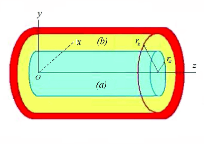
Figure 1: Cylindrical microscopic or mesoscopic tube: domain (a) of radius $r_{a}$ is occupied by air-vapor; domain (b) of external radius $r_{b}$ and internal radius $r_{a}$ is occupied by liquid-sap; the liquid-sap/air-vapor interface is the cylinder separating (a) and (b). Axis $x$ is horizontal, axis $y$ gives the upward direction of gravity and axis $z$ is the cylinder axis.

The perturbed liquid-sap/air-vapor interface $H$ of equation $H(r,\theta,z,t)=0$ can be written:

$$H(r,\theta,z,t)=r-r_{a}-\eta$$

where $\eta=\eta(\theta,z,t)$ denotes the dynamical displacement of the liquid-sap/air-vapor interface. From calculations obtained in Appendix A.1, we obtain Laplace’s relationship expanded to first order with respect to $\eta$ :

$$P_{a}(\eta)-P_{b}(\eta)=\gamma\left\{\frac{1}{r_{a}}-\frac{1}{r_{a}^{2}}\left(\eta+\eta^{\prime\prime}_{\theta^{2}}\right)-\eta^{\prime\prime}_{z^{2}}\right\}+\mathcal{O}(\eta^{2})$$ (6)

where ^′′ denotes the second order partial derivative with respect to $\theta$ or $z$,

II.0.3 Study of perturbations

The linearization of (3) and (5) at interface $r=r_{a}$ leads to a system with constant coefficients in $(z,t)$. The dependence of solutions in $z$ and $t$ is therefore exponential, and disturbances can be researched in normal modes of form Ruggeri (1995):

$$\left\{\begin{array}[]{l}{\phi_{j}}=\hat{\phi_{j}}(r,\theta)\,e^{i(kz-\omega t)}\\ \\ {p_{j}}=\hat{p_{j}}(r,\theta)\,e^{i(kz-\omega t)}\quad\qquad j\in\{a,b\}\\ \\ {\eta}=\hat{\eta}(\theta)\,e^{i(kz-\omega t)}\quad\,\,\ \quad\qquad{\rm at}\quad r=r_{a}\\ \end{array}\right.$$ (7)

where $k\in\mathbb{R}^{+\star}$ is the wave number, $\omega\in\mathbb{R}^{+\star}$ is the wave frequency. We denote by $\lambda=\displaystyle{2\pi}/{k}$ the wavelength.
At interface, we look for perturbations $\eta$  corresponding to wave frequency $\omega$ and we deduce:

$${\eta}(z,t)=\hat{\eta}\left(\theta\right)\,e^{i(kz-\omega t)}\quad\Longrightarrow\quad\ddot{\eta}(z,t)=-\omega^{2}{\eta}(z,t)$$

where  $\ddot{}=d^{2}/dt^{2}$  denotes the second order particular derivative. Then, perturbation ${\eta}$ verifies the differential equation:

$$\ddot{\eta}+\omega^{2}\,\eta=0$$ (8)

Likewise, we denote $[p]$ the discontinuity at interface liquid-sap/air-vapor of pressure $p$:

$$[p(z,t)]=\left(\,\hat{p_{a}}(r_{a},\theta)-\hat{p_{b}}(r_{a},\theta)\right)\,e^{i(kz-\omega t)}$$

Then,

$$[\ddot{p}]+\omega^{2}\,[p]=0$$ (9)

To be complete, in Appendix A.2, we prove that the velocities $\bm{u}_{j}$  in relation (2) and perturbations $\eta$  are compatible with motion equations (5) and boundary conditions.

II.0.4 Numerical applications and their consequences

The fluid in $(a)$ domain is air and vapor; the fluid in $(b)$ domain is crude or elaborated sap. The temperature is generally about $20\degree$ Celsius. In C.G.S. units, we have Weast (1984):

For the crude sap (which is mainly water with some salts):

$$\rho_{a}\simeq 0,\quad\rho_{b}\simeq 1,\quad\gamma\simeq 70$$

For the elaborated sap (for example maple syrup):

$$\rho_{a}\simeq 0,\quad\rho_{b}\simeq 1,34,\quad\gamma\simeq 70$$

For example, the sizes in the micro-channel are assumed to be:

$$r_{a}=2\times 10^{-3}{\rm cm}=20\,\mu{\rm m},\quad r_{b}=4\times 10^{-3}{\rm cm}=40\,\mu{\rm m}$$

For mesoscopic diameters, the obtained results will be even more accurate. The equation verified by values $k$ and $\omega$ of perturbations (7) is the result of Appendix A.2; we obtain:

$$\begin{array}[]{l}\displaystyle\omega^{2}\,\left(r_{a}\,\rho_{a}+\frac{r_{b}^{2n}r_{a}^{-n}+r_{a}^{n}}{r_{b}^{2n}r_{a}^{-n-1}-r_{a}^{n-1}}\,\rho_{b}\right)=\\ \displaystyle\qquad\qquad\qquad\gamma\,n\,\left(k^{2}+\frac{n^{2}-1}{r_{a}^{2}}\right)-n\,\left(\rho_{b}-\rho_{a}\right)\,g\,{\rm sin}\theta\end{array}$$ (10)

which is an extension of the Rayleigh–Taylor equation for planar interfaces Charru (2011).

$\bullet\quad$ if $n\geq 2,\ n\in\mathbb{N}$, then ${(n^{2}-1)}/{r_{a}^{2}}>7.5\,\times 10^{5}$. For any value of $g\ ({\rm where}\ g<10^{3}\ {\rm cm.s}^{-2})$,

$$(n^{2}-1)\,\frac{\gamma}{r_{a}^{2}}>5\times 10^{7}\gg\left(\rho_{b}-\rho_{a}\right)g\,\mid{\rm sin}\theta\mid$$

Consequently, for $n\geq 2$, in (10), the gravity has no influence on the perturbations along the interface. From (10) we obtain:

$$\gamma\,n\,k^{2}=\omega^{2}\left(\frac{r_{b}^{2n}r_{a}^{-n}+r_{a}^{n}}{r_{b}^{2n}r_{a}^{-n-1}-r_{a}^{n-1}}\,\rho_{b}\right)-\gamma\,n\,\left(\frac{n^{2}-1}{r_{a}^{2}}\right)$$

The values of $\omega$ such that

$$\omega^{2}\left(\frac{r_{b}^{2n}r_{a}^{-n}+r_{a}^{n}}{r_{b}^{2n}r_{a}^{-n-1}-r_{a}^{n-1}}\,\rho_{b}\right)-\gamma\,n\,\left(\frac{n^{2}-1}{r_{a}^{2}}\right)>0$$

are only possible. It can be immediately seen that $\omega$ corresponds to a period $T\ll 1$ s. As we will see in Section III, this period is not in our study range.

$\bullet\quad$ if $n=1$, the equation (10) yields:

$$\omega^{2}\,r_{a}\frac{r_{b}^{2}+r_{a}^{2}}{r_{b}^{2}-r_{a}^{2}}\,\rho_{b}=\gamma\,k^{2}-\,\rho_{b}\,g\,{\rm sin}\,\theta$$ (11)

It is necessary that $\gamma\,k^{2}$ and $\rho_{b}\,g\,{\rm sin}\,\theta$ are of the same order of magnitude. The most significant case corresponds to the micro-tube top where the effect of gravity is maximum:

$${\rm sin}\,\theta=1\quad\Longleftrightarrow\quad\theta=\frac{\pi}{2}$$

In this case, the terms $\gamma\,k^{2}$ and $\textbf{\,}\rho_{b}\,g$ are equal when the value $k=2\pi/\lambda$ is minimum equal to $k_{m}$ corresponding to $\lambda$ maximum and equal to $\lambda_{M}$, i.e.:

$$k_{m}=\sqrt{\frac{\rho_{b}\,g}{\gamma}}\quad\Longleftrightarrow\quad\lambda_{M}=2\pi\sqrt{\frac{\gamma}{\rho_{b}\,g}}$$

For a stable equilibrium position when $g$ is constant, $\omega^{2}$ must be positive. Consequently, due to the fact $r_{b}>r_{a}$ and $\omega^{2}>0$,

$$\gamma\,k^{2}-\rho_{b}\,g>0$$

For a liquid–gas plug length of less than $\lambda_{M}$, the fluids are stable in the Rayleigh–Taylor model. The oscillations have an angular frequency $\omega$ given by (11). The period of oscillation is $T=2\pi/\omega$. We obtain from equation (10):

$$k^{2}={\frac{\rho_{b}g}{\gamma}\left(1+\frac{\omega^{2}\,\gamma\,r_{a}\left(r_{b}^{2}+r_{a}^{2}\right)}{g\left(r_{b}^{2}-r_{a}^{2}\right)}\right)}\equiv{\frac{\rho_{b}g}{\gamma}\left(1+\frac{4\pi^{2}\,\gamma\,r_{a}\left(r_{b}^{2}+r_{a}^{2}\right)}{g\,T^{2}\left(r_{b}^{2}-r_{a}^{2}\right)}\right)}$$

Let us consider the case of an horizontal micro-channel on Earth. For $T>10^{3}$ s, $r_{a}<0.01$ cm, $r_{b}=1.1\,r_{a}$, then

$$\frac{\displaystyle 4\pi^{2}\gamma\,r_{a}}{\displaystyle g\,T^{2}}\frac{\displaystyle r_{b}^{2}+r_{a}^{2}}{\displaystyle r_{b}^{2}-r_{a}^{2}}<3\times 10^{-7}$$

is negligible with respect to 1. On Earth, $g=981\,{\rm cm.s}^{-2}$, we obtain $\lambda_{M}\simeq 1.68$ cm. This is the maximum size of fluid plug lengths.

We may extend the previous results for micro-channels inside the ISS. In ISS revolutions, the apparent gravity is less than $150\,\mu{\rm Gal}$ Barlow (2015). It is easy to verify that $\lambda_{M}$ is over hundred meters and the interface is always stable in Rayleigh–Taylor’s model. The perturbation of interfaces are always in form (7); calculations are similar, and (8) and (9) are always satisfied.

II.1 Stability of vertical micro-tubes

This case corresponds to stem xylem-channels on Earth. We consider a second toy-model constituted by a vertical cylindrical tube (with diameters a few tenths to a few tens of microns), filled with liquid-sap and air-vapor. The tube is connected with a liquid-sap reservoir (see Fig. 2). The liquid-sap rises at level $h$ and creates a liquid-sap/air-vapor interface (meniscus). Jurin’s law of capillarity writes:

$$h=\frac{2\,\gamma\,{\rm cos}\,\Theta}{r_{0}\,\rho_{b}\,g}$$ (12)

where $\rho_{b}$ is the liquid density and $\gamma$ is the sap surface tension. We note that if $g$ varies infinitesimally, this has no consequence on $h$-height of the meniscus. In fact (12) is only the equilibrium equation for fluids in tubes. Dynamic perturbations of the meniscus must be studied from equations of motions. We again assume that fluids are incompressible and with negligible viscosities; we consider meniscus perturbations $\eta$ in vertical direction. The calculus are simpler than in Section 2.1; we refer to Chapter 2 in Charru (2011).
The linearization of perturbation equations yields a similar form as (3) and (6) for meniscus displacements; it comes a system with coefficients independent of $r$ and $t$, where $r$ is the radial coordinate. The dependence of solutions in $r$ and $t$ is therefore exponential, and disturbances can be researched in form of normal modes. We obtain a representation in a form similar to Eq. (2.34) in Charru (2011), but with $r$ in place of $x$:

$$\left\{\begin{array}[]{l}{\phi_{j}}=\hat{\phi_{j}}(y),\,e^{i(kr-\omega t)}\\ \\ {p_{j}}=\hat{p_{j}}(y)\,e^{i(kr-\omega t)}\qquad j\in\{a,b\},\ k\in\mathbb{R}^{+\star}\ {\rm and}\,\ \omega\in\mathbb{R}^{+\star}\\ \\ {\eta}=\hat{\eta}(y)\,e^{i(kr-\omega t)}\\ \end{array}\right.$$

where domain $(a)$ corresponds to air-vapor and domain $(b)$ to liquid-sap.

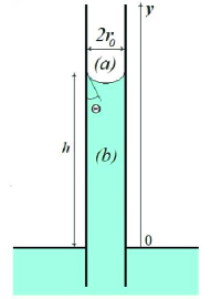
Figure 2: A vertical cylindrical micro-tube of radius $r_{0}$ is filled until level $h$ by the crude sap. Sap constant density is $\rho_{b}$; $\Theta$ is the Young contact angle of the meniscus with the micro-tube’s wall.

Perturbations ${\eta}$ at the interface again verify the differential equation:

$$\ddot{\eta}+\omega^{2}\,\eta=0$$

Discontinuity of pressure $[p]$ through the meniscus verifies: $[p(z,t)]=\left(\,\hat{p_{a}}-\hat{p_{b}}\right)\,e^{i(kz-\omega t)}$ and consequently:

$$[\ddot{p}]+\omega^{2}\,[p]=0$$

In the case of revolution of the Moon around the Earth, $g=981\,{\rm cm.s}^{-2}$ and we always obtain the capillary length $\lambda_{M}\simeq 1.68$ cm Charru (2011). Due to radius sizes of micro-channels, when $g$ is assumed constant, liquid-sap plugs always exist and meniscus is stable for the Rayleigh–Taylor model.

III Variations of gravity due to
the Moon and Sun

Relatively to fixed directions with respect to stars, the period $T$ of a satellite around the Earth and its corresponding angular frequency $\displaystyle\omega$ can be written Brouwer, Clemence (1961):

$$T=2\pi\sqrt{\frac{a^{3}}{R^{2}g}}\qquad{\rm and}\qquad\omega=\sqrt{\frac{R^{2}g}{a^{3}}}$$ (13)

where $g$ is the associated averaged acceleration of gravity on Earth, $R$ the Earth radius and $a$ the apogee lenght of the satellite orbit.

III.1 Variations of gravity on the Earth

On Earth, when the Moon is at its zenith, the gravity decreases by $110\,\mu$Gal (1 $\mu$Gal $=10^{-6}$ cm.s^-2); when the Moon is at the horizon, it decreases by 170 $\mu$Gal. The action of the Sun, which is 2.17 times weaker than the Moon action, causes a maximum variation of $80\,\mu$Gal under similar conditions. In the most favorable case the gravity undergoes a variation of $250\,\mu$Gal, corresponding to a variation of about 1/4 000 000 th of its intensity Gougenheim (1953); Longman (1959). The actual estimation of gravimetric–tide is provided by Kingelé’s Etide program Volkov (2012). However, due to the circulation of the Moon around the Earth over one month, the distance from Moon to Earth varies. The spacing between the two bodies does not significantly vary during one day; the value is given for a position along the lunar orbit (see Fig. 3).
The Moon moves around the Earth axis $O\bm{k}_{0}$ relatively to fixed directions with respect to stars during $T_{L}=27.3$ days. The associated angular frequency is $\displaystyle\omega_{L}=2\pi\times 4.24\times 10^{-7}$ rad.s^-1.
Relatively to fixed directions with respect to stars, the Earth rotates around axis $O\bm{k}_{0}$ during $T_{E}=$ 24 hours. The associated angular frequency is $\omega_{{}_{E}}=2\pi\times 1.16\times 10^{-5}$ rad.s^-1.
Relatively to Earth-bound axes of third axis $O\bm{k}_{0}$, the apparent Moon motion has a period of $\displaystyle T_{L_{E}}=24.8$ hours Barlow (2015). The associated angular frequency is $\omega_{L_{E}}=2\pi\times 1.12\times 10^{-5}$ rad.s^-1.
The gravity on Earth is not constant and its perturbation has a period which is associated with the apparent motion of the Moon around the Earth. A simple expression of the gravity variation on Earth can be written in periodic form as:

$$g(t)=g_{{}_{E}}\left(1+\varepsilon_{{}_{E}}{\rm cos}\left(\omega_{L_{E}}\,(t-t_{0})\right)\right),\quad g_{{}_{E}}=\frac{1}{T_{L_{E}}}\int_{0}^{T_{L_{E}}}g(t)dt$$

where $\varepsilon_{{}_{E}}=1.25\times 10^{-7}=$ 1/8 000 000 with $g_{{}_{E}}=9.81\times 10^{8}\mu$Gal. Because $g$ is associated with the Moon orbit in axes centered at the Earth and fixed directions with respect to stars, we obtain from (13):

$$\omega_{L}^{2}=\frac{R^{2}g(t)}{a^{3}}=\frac{R^{2}g_{{}_{E}}\left(1+\varepsilon_{{}_{E}}{\rm cos}\left(\omega_{L_{E}}\,(t-t_{0})\right)\right)}{a^{3}}$$

where $a$ is the Moon apogee relative to the Earth.

$$\omega_{L}^{2}=\omega_{L_{e}}^{2}\left(1+\varepsilon_{{}_{E}}{\rm cos}\left(\omega_{L_{E}}\,(t-t_{0})\right)\right)\quad{\rm with}\quad\omega_{L_{e}}^{2}=\frac{R^{2}g_{{}_{E}}}{a^{3}}$$

The revolutions being associated with the rotation around the axis $O\bm{k}_{0}$ of the plane containing $O\bm{k}_{0}$ and the Moon center, then   $\omega_{L_{E}}+\omega_{L}=\omega_{{}_{E}}$ and due to $\varepsilon_{{}_{E}}\ll 1$:

$$\omega_{L_{E}}=\omega_{{}_{E}}-\omega_{L}\equiv\omega_{{}_{E}}-\omega_{L_{e}}\left(1+\frac{\varepsilon_{{}_{E}}}{2}{\rm cos}\left(\omega_{L_{E}}\,(t-t_{0})\right)\right)$$

We denote $\omega_{L_{E_{0}}}=\omega_{{}_{E}}-\omega_{L_{e}}$. Due to the fact that $\omega_{L_{E_{0}}}\simeq\omega_{L_{E}}$, we obtain:

$$\omega_{L_{E}}^{2}=\omega_{L_{E_{0}}}^{2}\left(1+\varepsilon_{{}_{E_{0}}}{\rm cos}\left(\omega_{L_{E_{0}}}\,(t-t_{0})\right)\right)$$

where $\displaystyle\varepsilon_{{}_{E_{0}}}=\left(\omega_{L_{e}}/{\omega_{L_{E_{0}}}}\right)\varepsilon_{{}_{E}}=0.47\times 10^{-8}$.

III.2 Variations of gravity at the ISS altitude

Relatively to Earth-bound axes of third axis $O\bm{k}_{0}$, the ISS revolution has a period $T_{I_{E}}=93\ {\rm minutes}$. The ISS moves around axis $O\bm{k}_{0}$ with the same orientation than the Earth (trigonometric rotation), but $15.8$ times faster. The associated angular frequency is $\omega_{I_{E}}=2\pi\times 1.79\times 10^{-4}$ rad.s^-1.

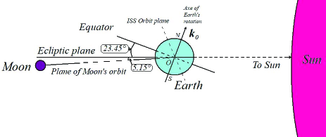
Figure 3: The Earth’s rotation around axis $\bm{k}_{0}$. The ISS orbit, the Moon and Sun positions are indicated on the figure.

Relative to fixed directions with respect to stars, the Earth rotates around axis $O\bm{k}_{0}$ in $T_{E}=$ 24 hours. The revolutions being associated with the rotation around the axis $O\bm{k}_{0}$ of the plane containing $O\bm{k}_{0}$ and the ISS, the ISS has a sidereal angular frequency (frequency relative to axes of fixed direction with respect to stars) $\omega_{I}=\omega_{I_{E}}+\omega_{E}=2\pi\times 1.91\times 10^{-4}$ rad.s^-1.

Variations of the lunisolar tidal acceleration in the ISS are closely sinusoidal Fisahn, Yazdanbakhsh, Klingelé, Barlow (2012); Fisahn, Klingelé, Barlow (2015). The gravitational oscillations expressed by the Etide program proposed by Klingelé, can be first found in Volkov (2012). The Etide program shows that the period of gravitational variations is about 45 minutes with two maxima of about $150\ \mu$Gal and two minima of about $-70\ \mu$Gal.

However, due to the circulation of the Moon around the Earth relative to axes of fixed directions with respect to stars during one month, the distance from Moon to Earth varies. Because the spacing between the two bodies does not significantly vary during 93 minutes, the value is given for a position when the ISS is at an altitude of 410 km. The perturbation term has a period which is the half of the revolution period around the Earth. We can write a simple expression of gravity at the ISS level (it is not the micro-gravity inside the ISS but the gravity due to the Earth-Moon-Sun):

$$g(t)=g_{I}\left(1+\varepsilon_{I}{\rm cos}\left(2\,\omega_{I_{E}}\,(t-t_{1})\right)\right),\ \ \,g_{I}=\frac{1}{T_{I_{E}}}\int_{0}^{T_{I_{E}}}g(t)\,dt$$

$g(t)$ is a periodic function of $t$ of period $T_{I_{E}}/2$ where $g_{I}=8.83\times 10^{8}\mu$Gal and $\varepsilon_{I}=1.25\times 10^{-7}$.
The gravity variation effect on $\omega_{I}$ is associated with the ISS orbit around the Earth relatively to axes of fixed directions with respect to stars (see Fig. 3):

$$\omega_{I}^{2}=\frac{g(t)}{a}=\frac{g_{I}\left(1+\varepsilon_{I}\,{\rm cos}\left(2\,\omega_{I_{E}}(t-t_{1})\right)\right)}{a}$$

where $a$ is the apogee length of the ISS with respect to the Earth and here $g(t)$ is the value of gravity at ISS level.

$$\omega_{I}^{2}=\omega_{I_{e}}^{2}\left(1+\varepsilon_{I}\,{\rm cos}\left(2\,\omega_{I_{E}}(t-t_{1})\right)\right)\quad{\rm with}\quad\omega_{I_{e}}^{2}=\frac{g_{I}}{a}$$

Due to the fact that $\varepsilon_{I}\ll 1$:

$$\omega_{I_{E}}=\omega_{I_{e}}\left(1+\frac{\varepsilon_{I}}{2}{\rm cos}\left(2\,\omega_{I_{E}}\,(t-t_{1})\right)\right)-\omega_{E}$$

We denote $\omega_{I_{E_{0}}}=\omega_{I_{e}}-\omega_{{}_{E}}$. From $\omega_{I_{E_{0}}}\simeq\omega_{I_{E}}$, we obtain:

$$\omega_{I_{E}}^{2}=\omega_{I_{E_{0}}}^{2}\left(1+\varepsilon_{I_{0}}{\rm cos}\left(2\,\omega_{I_{E_{0}}}(t-t_{1})\right)\right)$$

where $\varepsilon_{I_{0}}=\left({\omega_{I_{e}}}/{\omega_{I_{E_{0}}}}\right)\varepsilon_{I}$   and   $\varepsilon_{I_{0}}=1.34\times 10^{-7}$.

IV Instability of fluid-interfaces in microscopic or mesoscopic tubes submitted to periodic gravitational forces

IV.1 The Mathieu parametric resonance

Hill’s equation is the differential equation $\ddot{x}+f(t)\,x=0$, where $f(t)$ is a periodic function. Depending of $f(t)$, solutions may stay bounded at all times or the amplitude of oscillations may grow exponentially as described by Floquet’s theory Arnold (1989). An important case is Mathieu’s equation Mathieu (1868):

$$\ddot{x}+\omega_{0}^{2}\left(1+\varepsilon\cos(q\,\omega_{0}\,t)\right)\,x=0,$$ (14)

where $\omega_{0}\in\mathbb{R}^{+\star}$ is eigenfrequency of the system, $\varepsilon\in\mathbb{R}^{\star}$ is a small real parameter ($\left|\varepsilon\right|\ll 1$ ) and $q\in\mathbb{R}^{+\star}$ (we use the term $\omega_{0}$ as angular frequency and $\varepsilon$ with the same meaning than in Section III). This case corresponds to a differential equation of motion of a pendulum whose frequency $\omega=\omega_{0}\sqrt{1+\varepsilon\cos(q\,\omega_{0}\,t)}$ varies over time. The fundamental pendulum period is $\displaystyle T_{0}={2\pi}/{\omega_{0}}$. The system of Hamilton equations corresponding to (14) can be associated with a point of the plane constituted of couples $\left\{q,\varepsilon\right\}$ (see Fig. 4). We have the fundamental Mathieu theorem:

Theorem: Points of $q$-axis corresponding to $\varepsilon=0$ are stable, except points $\displaystyle q={2}/{p}$, where $\,p\in\mathbb{N}$, which are unstable.

The proof of the theorem is given in Arnold (1989); Gouin (2020). As small as $\varepsilon$ is, the theorem proves that the amplitude of oscillations of $x$ exponentially growths when $\displaystyle q={2}/{p},\ p\in\{1,2\}$.

The domain of instability of Mathieu’s equation in plane of couples $\left\{{1}/{q},\varepsilon\right\}$ contacts ${1}/{q}$-axis at points $\left\{\displaystyle{1}/{q}={p}/{2},\ p\in\mathbb{N}\right\}$. The corresponding values of ${p}/{2}$ on ${1}/{q}$-axis are called points of parametric resonance. For plane red domains in Fig. 4 the solutions of (14) become unstable. This parametric resonance is strongest manifesting when $p=1$ or ($q=2$). Parametric resonance really manifests for $q=2,\,q=1$ and more rarely for $q=2/3$.

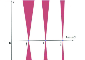
Figure 4: Instability domains in the parametric resonance case.

IV.2 Influence of the lunisolar-tidal’s resonance on plants

As seen in Section 3, the gravity is not constant during revolutions of the Moon and the ISS around the Earth. The liquid considered in toy-models is sap. On Earth, horizontal microscopic or mesoscopic tubes schematize plant root channels; vertical tubes schematizes stem channels. Inside the ISS, toy-model of Section II.1 schematizes roots and stems filled by sap. The channels are tubes of xylem or cells conducting water, crude sap, or elaborated sap, mixed with air-vapor. Equations (8) and (9) are modified by lunisolar-tides to obtain Mathieu’s equations.

IV.2.1 Resonances on the Earth

From Section 3,  $\omega_{L_{E_{0}}}=2\pi\times 1.12\times 10^{-5}$ rad.s^-1, $\displaystyle T_{L_{E}}=24.8$ hours and $\displaystyle\varepsilon_{{}_{E_{0}}}=0.47\times 10^{-8}$.
Perturbations ${\eta}$ associated with Moon revolutions around Earth-bound axes verifies $\ddot{\eta}+\omega_{L_{E}}^{2}\,\eta=0,$ but angular frequency $\omega_{L_{E}}$ is not constant and the differential equation (8) writes:

$$\ddot{\eta}+\omega_{L_{{}_{E0}}}^{2}\left(1+\varepsilon_{{}_{E_{0}}}{\rm cos}\left(\omega_{L_{E_{0}}}\,(t-t_{0})\right)\right)\,\eta=0$$

The perturbations of pressure through the liquid-sap/air-vapor interface verify the differential equation (9):

$$[\ddot{p}]+\omega_{L_{E_{0}}}^{2}\left(1+\varepsilon_{{}_{E_{0}}}{\rm cos}\left(\omega_{L_{E_{0}}}\,(t-t_{0})\right)\right)\,[p]=0$$

We are in the case $q=1$ of Eq. (14) corresponding to a small but effective impulsion.

IV.2.2 Resonances inside the ISS

From Section 3,  $\omega_{I_{E_{0}}}=2\pi\times 1.79\times 10^{-4}$ rad.s^-1, $T_{I_{E}}=93\ {\rm minutes}$ and $\varepsilon_{I_{0}}=1.34\times 10^{-7}$.
Perturbation ${\eta}$ associated with revolutions of the ISS around Earth-bound axes verifies $\ddot{\eta}+\omega_{I_{E}}^{2}\,\eta=0,$ but frequency $\omega_{I_{E}}$ is not constant and the differential equation (8) writes:

$$\ddot{\eta}+\omega_{I_{E_{0}}}^{2}\left(1+\varepsilon_{I_{0}}{\rm cos}\left(2\,\omega_{I_{E_{0}}}\,(t-t_{1})\right)\right)\,\eta=0$$

The perturbations of pressure through the liquid-sap/air-vapor interface verify the differential equation:

$$[\ddot{p}]+\omega_{I_{E_{0}}}^{2}\left(1+\varepsilon_{I_{0}}{\rm cos}\left(2\,\omega_{I_{E_{0}}}\,(t-t_{1})\right)\right)\,[p]=0$$

We are in case $q=2$ of Eq. (14) corresponding to a bigger impulsion than for Earth case.

The results come from periodic gravity variations of period commensurable with period of revolution of the Moon around Earth-bound axes. It can be seen in papers by Barlow et al that the effect of gravity variations on plants is steeper for the ISS since bean leaves oscillate dramatically. This observation is in accordance with Mathieu’s equations: the period of revolution of the ISS is much shorter than period of revolution of the Moon around the Earth and coefficient $\varepsilon$ in Mathieu’s equation is 35 times larger than the one associated with gravity variations on Earth. In addition, the resonance coefficient $q$ is optimum since the period of gravity variations in the ISS is half of its circumterrestrial revolution.

V Discussion and conclusion

The instabilities of fluid interfaces in microscopic or mesoscopic tubes subjected to periodic gravity come from Mathieu’s equations. As the variations of gravity are periodic and commensurable with the periods of revolution of the Moon or the ISS around the Earth’s axes, the instabilities always appear during rotation of the Earth and revolution of the ISS.
Inside the ISS, it can be seen that effects on plants are stronger than on Earth since leaves dramatically oscillate depending along the ISS’ cycle. Despite its extreme smallness, the variation of gravity on Earth has great consequences on ocean tides. The effect is less spectacular on plants. It is proven that disturbances of Mathieu’s equation exponentially increase over time Arnold (1989); then, the successive rotations of the ISS and Moon around the Earth amplify observed perturbations.

The lunar orbit relative to the Earth is not circular but elliptical with apogee of 405 400 km and perigee of 362 600 km. This fact was not taken into account in our calculations because the spacing between the two bodies does not vary significantly during $93$ minutes or one day. The gravity variation depending on this distance, we can assume that effects on plants and living organisms depend on the rising Moon and the falling Moon as Tavener’s gardener thinks Tavenner (1918).

Also at a mesoscopic level, interfacial capillarity is one of the main drivers of the rise of crude sap in trees Gouin (2015, 2017). It provokes, by pressure variations and time-exponential disturbances, lengthening of stems and swelling of roots. It can be assumed that the same phenomenon occurs in cells and thus explains the influence of lunisolar tide on all living organisms including animals and humans as predicted by Miles, Raynal, Wilson (1977); Gluckman, Netoff, Neel, Ditto, Spano, Schiff (1996). In astronomy, orbital resonances appear; the periodic gravitational influence may destabilize the orbits of asteroids Brouwer, Clemence (1961). Thus, in the whole of nature, at nanoscopic, microscopic, metric, terrestrial and sidereal scales, materials and creatures are subject to gravitational resonance phenomena.

We have only considered instabilities due to lunisolar tides without developing information on the dynamics of the induced flows. Such an important development could be the subject of voluminous numerical computations. One could thus apply the Rayleigh-Taylor model for compressible fluids Bian (2020) or for incompressible fluid turbulence Boffetta (2017).

Data Availability Statement: The data that supports the findings of this study are available within the article and its bibliography.

Acknowledgments: The author is partially supported by CNRS, GDR PhyP: Bio-mécanique et biophysique des plantes and by Agence Nationale de la Recherche, France (project SNIP ANR–19–ASTR–0016–01).
I would like to thank Robert Findling, Sergey Gavrilyuk, and anonymous referees for their helpful comments and remarks.

Appendix A Compatibility with equations of motion and boundary conditions

The purpose of this appendix is to show that the system (7) and the equations (8) and (9) are compatible with the equations of motion (5).

A.1 Interfacial perturbations

From

$$dH=\frac{\partial H}{\partial t}dt+{\rm grad}H\,\bm{.}\,d\bm{M}\quad{\rm with}\quad d\bm{M}=\bm{w}\,dt$$

where $\bm{w}$ is the fluid velocity along the interface, we get:

$$\frac{\partial H}{\partial t}=-{\rm grad}H\,\bm{.}\,\bm{w}\qquad{\rm with}\qquad\frac{\partial H}{\partial t}=-\frac{\partial\eta}{\partial t}$$ (15)

In cylindrical coordinates:

$${\rm grad}\,H=\bm{e}_{r}-\frac{1}{r}\frac{\partial\eta}{\partial\theta}\bm{e}_{\theta}-\frac{\partial\eta}{\partial z}\bm{e}_{z}$$

where $\bm{e}_{r}$, $\bm{e}_{\theta}$ and $\bm{e}_{z}$ are the unit vectors of coordinate-lines. The external unit normal-vector to the interface is:

$$\bm{n}=\displaystyle\frac{\displaystyle\bm{e}_{r}-\frac{1}{r}\frac{\partial\eta}{\partial\theta}\bm{e}_{\theta}-\frac{\partial\eta}{\displaystyle\partial z}\bm{e}_{z}}{\displaystyle\sqrt{1+\frac{1}{r^{2}}\left(\frac{\partial\eta}{\partial\theta}\right)^{2}+\left(\frac{\partial\eta}{\partial z}\right)^{2}}}$$

From (15) we deduce:

$$\bm{w}\,.\,\bm{n}=\frac{\displaystyle\frac{\partial\eta}{\partial t}}{\displaystyle\sqrt{1+\frac{1}{r^{2}}\left(\frac{\partial\eta}{\partial\theta}\right)^{2}+\left(\frac{\partial\eta}{\partial z}\right)^{2}}}$$ (16)

For fluids in $(a)$ and $(b)$ domains, we write:

$$\bm{u}_{j}=\frac{\partial\phi_{j}}{\partial r}\bm{e}_{r}+\frac{1}{r}\frac{\partial\phi_{j}}{\partial\theta}\bm{e}_{\theta}+\frac{\partial\phi_{j}}{\partial z}\bm{e}_{z}\qquad j\in\{a,b\}$$

and from (15), (16), we get interfacial conditions:

$$\frac{\partial\phi_{j}}{\partial r}-\frac{1}{r^{2}}\frac{\partial\phi_{j}}{\partial\theta}\frac{\partial\eta}{\partial\theta}-\frac{\partial\phi_{j}}{\partial z}\frac{\partial\eta}{\partial z}=\frac{\partial\eta}{\partial t}\qquad j\in\{a,b\}$$ (17)

The sum $\mathcal{H}$ of principal curvature radii of liquid-sap/air-vapor interface is ${\mathcal{H}}={\rm div}\,\bm{n}$  Aleksandrov, Zalgaller (1967). Therefore,

$$\mathcal{H}=\frac{2}{\left(r^{2}+\eta^{\prime 2}_{\theta}+r^{2}\eta^{\prime 2}_{z}\right)^{0.5}}-\frac{r^{2}\left(1+\eta^{\prime 2}_{z}\right)}{\left(r^{2}+\eta^{\prime 2}_{\theta}+r^{2}\eta^{\prime 2}_{z}\right)^{1.5}}$$

$$-\frac{\eta^{\prime\prime}_{\theta^{2}}}{r\left(r^{2}+\eta^{\prime 2}_{\theta}+r^{2}\eta^{\prime 2}_{z}\right)^{0.5}}+\frac{\eta^{\prime}_{\theta}}{r}\frac{\eta^{\prime}_{\theta}\eta^{\prime\prime}_{\theta^{2}}+r^{2}\eta^{\prime}_{z}\eta^{\prime\prime}_{z\theta}}{\left(r^{2}+\eta^{\prime 2}_{\theta}+r^{2}\eta^{\prime 2}_{z}\right)^{1.5}}$$

$$-\frac{r\eta^{\prime\prime}_{z^{2}}}{\left(r^{2}+\eta^{\prime 2}_{\theta}+r^{2}\eta^{\prime 2}_{z}\right)^{0.5}}+\frac{r\eta^{\prime}_{z}\left(\eta^{\prime}_{\theta}\eta^{\prime\prime}_{\theta z}+r^{2}\eta^{\prime}_{z}\eta^{\prime\prime}_{z^{2}}\right)}{\left(r^{2}+\eta^{\prime 2}_{\theta}+r^{2}\eta^{\prime 2}_{z}\right)^{1.5}}$$

By expanding to first order with respect to $\eta$ expression of $\mathcal{H}$, we obtain for total curvature on the perturbed interface:

$$\mathcal{H}=\frac{1}{r_{a}}-\frac{1}{r_{a}^{2}}\left(\eta+\eta^{\prime\prime}_{\theta^{2}}\right)-\eta^{\prime\prime}_{z^{2}}+\mathcal{O}(\eta^{2})$$

A.2 Compatibility with motion equations

A.2.1 The incompressibility

Equation of incompressibility (3) yields:

$$\left(\frac{1}{r}\,\frac{\partial{\hat{\phi_{j}}}}{\partial r}+\frac{\partial^{2}{\hat{\phi_{j}}}}{\partial r^{2}}+\frac{1}{r^{2}}\frac{\partial^{2}{\hat{\phi_{j}}}}{\partial\theta^{2}}-k^{2}\hat{\phi_{j}}\right)\,e^{i(kz-\omega t)}=0$$

which is equivalent to:

$$r^{2}\,\frac{\partial^{2}{\hat{\phi_{j}}}}{\partial r^{2}}+r\frac{\partial{\hat{\phi_{j}}}}{\partial r}-k^{2}r^{2}\hat{\phi_{j}}+\frac{\partial^{2}{\hat{\phi_{j}}}}{\partial\theta^{2}}=0$$ (18)

Classically, we look for solutions of (18) in form:

$$\hat{\phi_{j}}(r,\theta)=\varphi_{j}(r)\,\psi_{j}(\theta)$$

We obtain:

$$\frac{r^{2}\,{\varphi_{j}}^{\prime\prime}(r)+r{\varphi_{j}}^{\prime}(r)-k^{2}r^{2}\,{\varphi_{j}}(r)}{{\varphi_{j}}(r)}+\frac{{\psi_{j}}^{\prime\prime}(\theta)}{{\psi_{j}}(\theta)}=0$$

$\bullet\quad$ Consequently, there exist two real constants $\alpha_{j},\ j\in\{a,b\}$ such that:

$$\frac{{\psi_{j}}^{\prime\prime}(\theta)}{{\psi_{j}}(\theta)}=-\alpha_{j}\quad\Longleftrightarrow\quad{\psi_{j}}^{\prime\prime}(\theta)+\alpha_{j}{\psi_{j}}(\theta)=0$$

Due to the cylindrical geometry of tubes, ${\psi_{j}}(\theta)$ must be periodic with a period which is a divider of $2\pi$. Then, $\alpha_{j}=n_{j}^{2}$ where $n_{j}\in\mathbb{N}^{\star}$, and

$${\psi_{j}}(\theta)=A_{j}{\rm sin}(n_{j}(\theta-\theta_{0j}))\quad{\rm with}\quad\theta_{0j}\,\ {\rm and}\,\ A_{j}\in\mathbb{R}$$

$\bullet\quad$ Furthermore:

$$r^{2}\,{\varphi_{j}}^{\prime\prime}(r)+r{\varphi_{j}}^{\prime}(r)-(n_{j}^{2}+k^{2}r^{2})\,{\varphi_{j}}(r)=0$$ (19)

with $\displaystyle k\,r\leq k\,r_{b}$. Due to diameter channel sizes, we assume that $r_{b}\ll\lambda$, and consequently $k^{2}r^{2}\ll 1$. So, (19) can be linearized in the form:

$$r^{2}\,{\varphi_{j}}^{\prime\prime}(r)+r{\varphi_{j}}^{\prime}(r)-n_{j}^{2}\,{\varphi_{j}}(r)=0$$ (20)

Solutions of (18) are:

$${\hat{\phi_{j}}}(r,\theta)=\left(A_{j}\,r^{n_{j}}+B_{j}\,r^{-n_{j}}\right)\,{\rm sin}\left(n_{j}\left(\theta-\theta_{0j}\right)\right)$$ (21)

with $A_{j}\,\ {\rm and}\,\ B_{j}\in\mathbb{R}$. Terms ${\partial\eta}/{\partial\theta},\ {\partial{\phi_{j}}}/{\partial\theta},\ {\partial\eta}/{\partial z},\ {\partial{\phi_{j}}}/{\partial z}$ are small quantities and consequently their products are negligible. From (17) we deduce ${\partial{\phi_{j}}}/{\partial r}={\partial{\eta}}/{\partial t},\ j\in\{a,b\}$. From

$$\frac{\partial{\phi_{j}}}{\partial r}=\frac{\partial{\hat{\phi_{j}}}}{\partial r}\,e^{i(kz-\omega t)}\quad{\rm and}\quad\displaystyle\frac{\partial{\eta}}{\partial t}=-\eta\,i\,\omega\equiv-\hat{\eta}\,i\,\omega\,e^{i(kz-\omega t)}$$

we deduce for $r=r_{a}$:

$$\ \frac{\partial{\hat{\phi_{j}}}}{\partial r}=-\hat{\eta}\,i\,\omega\qquad\quad j\in\{a,b\}$$ (22)

From (5) linearized, $\rho_{j}\,({\partial\phi_{j}}/{\partial t})+p_{j}=0$ and we obtain:

$$-i\,\omega\,\rho_{j}{\hat{\phi_{j}}}+{\hat{p_{j}}}=0\qquad\quad j\in\{a,b\}$$ (23)

As in Charru (2011), to linearize Laplace’s relationship near $r=r_{a}$, we consider a Young–Taylor expansion at $\eta=0$. For a given value of $\theta$, we obtain:

$$P_{j}(\eta)=\overline{{P_{j}}(\eta)}+p_{j}(\eta)=\overline{{P_{j}}(0)}+\eta\frac{\partial}{\partial r}\left({{P_{j}}(\eta)}\right)_{\eta=0}+p_{j}(0)+\mathcal{O}(\eta^{2})$$

From ${{P_{j}}(\eta)}={\overline{{P_{j}}(0)}}-\rho_{j}g\,y\equiv{\overline{{P_{j}}(0)}}-\rho_{j}g\,r\,{\rm sin}\theta$, we get ${\partial{{P_{j}}(\eta)}}/{\partial r}=-\rho_{j}g\,{\rm sin}\theta$ and finally:

$${{P_{j}}(\eta)}={\overline{{P_{j}}(0)}}-\eta\,\rho_{j}g\,{\rm sin}\theta+p_{j}(0)$$

We denote $p_{a}$ and $p_{b}$ for $p_{a}(0)$ and $p_{b}(0)$. Consequently,

$$P_{a}(\eta)-P_{b}(\eta)={\overline{{P_{a}}(0)}}-{\overline{{P_{b}}(0)}}-\eta\,\rho_{a}g\,{\rm sin}\theta+\eta\,\rho_{b}g\,{\rm sin}\theta+p_{a}-p_{b}$$

From (6), ${\overline{{P_{a}}(0)}}-{\overline{{P_{b}}(0)}}={\gamma}/{r_{a}}$, and we obtain the equation:

$$\left(\eta\,\rho_{b}g\,{\rm sin}\theta-p_{b}\right)-\left(\eta\,\rho_{a}g\,{\rm sin}\theta-p_{a}\right)=-\gamma\left\{\frac{1}{r_{a}^{2}}\left(\eta+\eta^{\prime\prime}_{\theta^{2}}\right)+\eta^{\prime\prime}_{z^{2}}\right\}$$ (24)

From $\left({\partial{\hat{\phi_{j}}}}/{\partial r}\right)_{r=r_{a}}=f(r_{a})\,{\rm sin}\left(n_{j}\left(\theta-\theta_{j0}\right)\right)$ where $f$ is solution of (20) and from (22), we obtain:

$$\hat{\eta}=h(\omega,r_{a})\,{\rm sin}\left(n_{j}\left(\theta-\theta_{j0}\right)\right)$$

where $h$ is a convenient function related to $f$. Displacement ${\hat{\eta}}$ being independent of $j\in\{a,b\}$, we have $n_{a}=n_{b}\equiv n$ and $\theta_{a0}=\theta_{b0}=\theta_{0}$. Then,

$$\hat{\eta}^{\prime\prime}_{\theta^{2}}=-n^{2}h(\omega,r_{a})\,{\rm sin}\left(n\left(\theta-\theta_{0}\right)\right)\quad\Longrightarrow\quad\hat{\eta}^{\prime\prime}_{\theta^{2}}=-n^{2}\,\hat{\eta}$$

A.2.2 Boundary conditions

In cylindrical coordinates:

$$\bm{u}_{j}={\rm grad}\,\phi_{j}=\frac{\partial\phi_{j}}{\partial r}\,\bm{e}_{r}+\frac{1}{r}\,\frac{\partial\phi_{j}}{\partial\theta}\,\bm{e}_{\theta}+\frac{\partial\phi_{j}}{\partial z}\,\bm{e}_{z}$$

where $j\in\{a,b\}$, and with expression (21):

$$\left\{\begin{array}[]{l}\displaystyle\frac{\partial{\phi_{j}}}{\partial r}=n\,\left(\,A_{j}\,r^{n-1}-\,B_{j}\,r^{-n-1}\right)\,{\rm sin}\left(n(\theta-\theta_{0})\right)e^{i(kz-\omega t)}\\ \\ \displaystyle\frac{1}{r}\,\frac{\partial{\phi_{j}}}{\partial\theta}=\left(\,A_{j}\,r^{n-1}+B_{j}\,r^{-n-1}\right)\,n\,{\rm cos}\left(n(\theta-\theta_{0})\right)e^{i(kz-\omega t)}\\ \\ \displaystyle\frac{\partial{\phi_{j}}}{\partial z}=\left(\,A_{j}\,r^{n}+\,B_{j}\,r^{-n}\right)\,{\rm sin}\left(n(\theta-\theta_{0})\right)i\,k\,e^{i(kz-\omega t)}\end{array}\right.$$

The components of $\bm{u}_{a}$ must be bounded in $(a)$ domain. Then $B_{a}=0$ and $\phi_{a}=A_{a}\,r^{n}\,{\rm sin}\left(n(\theta-\theta_{0})\right)e^{i(kz-\omega t)}\ {\rm with}\ n\in\mathbb{N}^{\star}$.
On the micro-tube’s wall $r=r_{b}$, the normal component of liquid velocity in domain $(b)$ is zero: on $r=r_{b}$, $\bm{u}_{b}\,\bm{.}\,\bm{e}_{r}=0$. Then, $\displaystyle\left({\partial{\phi_{b}}}/{\partial r}\right)_{r=r_{b}}=0$.
From  ${\partial{\phi_{b}}}/{\partial r}=n\,\left(\,A_{b}\,r^{n-1}-\,B_{b}\,r^{-n-1}\right)\,{\rm sin}\left(n(\theta-\theta_{0})\right)e^{i(kz-\omega t)}$, we obtain $B_{b}=A_{b}\,r_{b}^{2n}$. Condition (22) at $r=r_{a}$ implies:

$$\left(\frac{\partial{\phi_{a}}}{\partial r}\right)_{r=r_{a}}=\left(\frac{\partial{\phi_{b}}}{\partial r}\right)_{r=r_{a}}\,\ \Longrightarrow\,\ A_{a}\,r_{a}^{n-1}=A_{b}\,\left(r_{a}^{n-1}-r_{b}^{2n}r_{a}^{-n-1}\right)$$

and finally with $A=A_{b}$, $A_{a}=A\,\left(1-r_{a}^{-2n}r_{b}^{2n}\right)$:

$$\left\{\begin{array}[]{l}\displaystyle{\phi_{a}}=A\,\left(1-r_{a}^{-2n}r_{b}^{2n}\right)\,r^{n}{\rm sin}\left(n(\theta-\theta_{0})\right)e^{i(kz-\omega t)}\\ \\ \displaystyle{\phi_{b}}=A\,\left(1+r^{-2n}r_{b}^{2n}\right)\,r^{n}{\rm sin}\left(n(\theta-\theta_{0})\right)e^{i(kz-\omega t)}\end{array}\right.$$ (25)

A.2.3 Equation of pertubations

From (23) we have $\hat{p_{a}}=i\,\omega\,\rho_{a}\,\hat{\phi_{a}}$; from (LABEL:instabil) we obtain $\hat{\phi_{a}}=A_{a}\,r^{n}{\rm sin}\left(n(\theta-\theta_{0})\right)$, and from (22), for $r=r_{a}$:

$$A_{a}=-\frac{i\,\omega\,\hat{\eta}}{n\,r_{a}^{n-1}{\rm sin}\left(n\,(\theta-\theta_{0})\right)}$$

and from $\hat{p_{a}}=i\,\omega\,\rho_{a}A_{a}\,r^{n}{\rm sin}\left(n(\theta-\theta_{0})\right)$, we deduce at $r=r_{a}$:

$$\hat{p_{a}}=\frac{\omega^{2}\rho_{a}}{n}\,r_{a}\hat{\eta}$$

Likewise, from (23), we have $\hat{p_{b}}=i\,\omega\,\rho_{b}\,\hat{\phi_{b}}$; from (LABEL:instabil):

$$\hat{\phi_{b}}=A(r^{n}+r_{b}^{2n}r^{-n})\,{\rm sin}\left(n(\theta-\theta_{0})\right)$$

From (22), for $r=r_{a}$:

$$A=-\frac{i\,\omega\,\hat{\eta}}{n(r^{n-1}_{a}-r_{b}^{2n}r^{-n-1}_{a})\,{\rm sin}\left(n\,(\theta-\theta_{0})\right)}$$

From $\hat{p_{b}}=i\,\omega\,\rho_{b}A\,(r^{n}+r_{b}^{2n}r^{-n})\,{\rm sin}\left(n(\theta-\theta_{0})\right)$, we deduce at $r=r_{a}$:

$$\hat{p_{b}}=\frac{\omega^{2}\rho_{b}}{n}\frac{r_{a}^{n}+r_{b}^{2n}r_{a}^{-n}}{r_{a}^{n-1}-r_{b}^{2n}r_{a}^{-n-1}}\,\hat{\eta}$$

and from (24), we obtain the equation (10) of II.4 for possible perturbations at the interface in cylindrical micro-tubes.

References

- Moran (2007) N. Moran, FEBS Letters, 581, 2337 (2007).
- Bünning (1973) E. Bünning, The physiological clock. Circadian rhythms and biological chronometry, 3rd edition, English Universities Press, London (1973).
- Tavenner (1918) E. Tavenner E, Transactions and Proceedings of the American Philological Association, 49, 67, 1918. Published by The Johns Hopkins University Press, Baltimore, https://www.jstor.org/stable/282995
- Engelmann (2009) W. Engelmann, Clocks which run according to the moon influence of the moon on the earth and its life, 4th edition, Tobias-lib, University library, Tübingen (2009). http://tobias-lib.ub.uni-tuebingen.de/doku/lizenzen/xx.html
- Fisahn, Barlow, Dorda (2018) J. Fisahn, P. W. Barlow and G. Dorda, Annals of Botany, 122, 725 (2018).
- Gonen, Walz (2006) T. Gonen and T. Walz, Quarterly Review of Biophysics, 39, 361 (2006).
- Barlow (2015) P.W. Barlow, Annals of Botany, 116, 149 (2015).
- Klein (2007) G. Klein G, Farewell to the internal clock. A contribution in the field of chronobiology. Springer, New York (2007).
- Fisahn, Yazdanbakhsh, Klingelé, Barlow (2012) J. Fisahn, N. Yazdanbakhsh, E. Klingelé and P.W. Barlow, New Phytologist, 195, 346 (2012).
- Konopliv, Binder, Hood, Kucinskas, Sjogren, Williams (1998) A.S. Konopliv, A.B. Binder, L.L. Hood, A.B. Kucinskas, L. Sjogren and J.G. Williams, Science, 281, 1476 (1998).
- Konopliv, Asmar, Carranza, Sjogren, Yuan (2001) A.S. Konopliv, S.W. Asmar, E. Carranza, W.L. Sjogren and D.N. Yuan, Icarus, 150, 1 (2001).
- Gallep, Moraes, dos Santos, Barlow (2012) C.M. Gallep, T.A. Moraes, S.R. dos Santos and P.W. Barlow Protoplasma, 250, 793 (2012).
- Gallep, Moraes, Cervinkova, Cifra, Katsumata, Barlow (2012) C.M. Gallep, T.A. Moraes, K. Cervinkova, M. Cifra, M. Katsumata and P.W. Barlow. Plant Signaling and Behavior, 9, e28671 (2012).
- Harmer (2009) S.M. Harmer, Ann. Rev. Plant Biol., 60, 357 (2009).
- James, Monreal, Nimmo, Kelly, Herzyk, Jenkins, Nimmo (2008) A.B. James, J.A. Monreal, G.A. Nimmo, C.L. Kelly, P. Herzyk, G.I. Jenkins and H.G. Nimmo, Science, 322, 1832 (2008).
- Beeson (1946) C.F.C. Beeson Nature, 58, 572 (1946).
- Sorbetti-Guerri, Michel (1998) F. Sorbetti-Guerri and D. Michel, Nature, 392, 665 (1998).
- Zajaczhowska, Barlow (2017) U. Zajaczhowska and P.W. Barlow, Plant Biology, 19, 630 (2017).
- Xu, Sun, Ducarme (2004) J. Xu, H. Sun, B.A. Ducarme, Journal of Geodynamics, 38, 293 (2004).
- Crossley, Hinderer, Boy (2005) D. Crossley, J. Hinderer and J.P. Boy, Geophysical Journal International, 161, 257 (2005).
- Palmer (1995) J.D. Palmer, Chronobiology International, 12, 299 (1995).
- Miles, Raynal, Wilson (1977) L.E.M. Miles, D.M. Raynal and M.A. Wilson, Science, 198, 421 (1977).
- Gluckman, Netoff, Neel, Ditto, Spano, Schiff (1996) B.J Gluckman, T.I. Netoff, E.J. Neel, W.L. Ditto, M.L. Spano and S.J Schiff, Phys. Rev. Letters, 77, 4098 (1996).
- Brinckman (2005) E. Brinckman, Adv. Space. Res., 36, 1162 (2005).
- Bobst (2015) K. Bobst, How the Moon’s gravity influences Earth. Mother nature network. https://www.mnn.com/earth-matters/space/stories/how-moons-gravityinfluences-earth
- Jacob (2015) A. Jacob, Moon’s gravity could govern plant movement like the tides. New Scientist Daily News. https://www.newscientist.com/article/dn28051-moons-gravity-could-govern-plant-movement-like-the-tides/
- Fisahn, Klingelé, Barlow (2015) J. Fisahn, E. Klingelé and P.W. Barlow, Planta, 241, 1509 (2015).
- Solheim, Johnson, Iversen (2009) B.G.B. Solheim, A. Johnson and T.H. Iversen, New Phytol., 183, 1043 (2009).
- Chandrasekhar (1961) S. Chandrasekhar, Hydrodynamic and Hydromagnetic Stability. Dover Pub., New York (1961).
- Charru (2011) F. Charru, Hydrodynamic Instabilities. Cambridge Univ. Press (2011).
- Arnold (1992) V.I. Arnold, Ordinary Differential Equations, Springer, Berlin (1992).
- Mattia, Gogotsi (2008) D. Mattia and Y. Gogotsi Y, Microfluid-Nanofluid, 5, 289 (2008).
- Gouin (2012) H. Gouin, Note Mat., 32, 105 (2012).
- Seadawy (2016) A.R. Seadawy and K. El-Rashidy, Pramana, Springer, 87, 20 (2016).
- Hu (2019) Z.X. Hu, Y.S. Zhang, B. Tian, Z. He and L. Li, Physics of Fluids, 31, 104108 (2019).
- Landau, Lifchitz (1958) L. Landau and E. Lifchitz, Fluid Mechanics, Mir Edition, Moscow (1958).
- de Gennes, Brochard-Wyart, Quéré (2004) P.G. de Gennes, F. Brochard-Wyart and D. Quéré, Capillarity and Wetting Phenomena: Drops, Bubbles, Pearls, Waves, Springer, New York (2004).
- Ruggeri (1995) T. Ruggeri, Stability and wave propagation in fluids and solids, CISM Courses and Lectures N0 344, Ed. G.P. Galdi, p.p. 105-154, Springer, New York (1995).
- Weast (1984) Weast RC (Ed.), Handbook of Chemistry and Physics, 65th edition, CRC Press, Boca Raton, FLorida (1984).
- Brouwer, Clemence (1961) D. Brouwer and G.M. Clemence, Methods of Celestial Mechanics, Academic Press, New York (1961).
- Gougenheim (1953) A. Gougenheim, Lecture at Sixth International Hydrographic Conference, Monaco, pp. 22-27, (April–May 1952).
- Longman (1959) I.M. Longman, Journal of Geophysical Research, 64,2351 (1959).
- Volkov (2012) A.G. Volkov (Ed.), Plant Electrophysiology – Signaling an Responses, p.p. 249-279, Springer, Heidelberg (2012).
- Arnold (1989) V.I. Arnold, Mathematical Methods of Classical Mechanics, Springer, Berlin (1989).
- Mathieu (1868) E. Mathieu, Journal de mathématiques pures et appliquées, 13, 137 (1868).
- Gouin (2020) H. Gouin, Introduction to Mathematical Methods of Analytical Mechanics, Elsevier & ISTE Editions, London (2020).
- Gouin (2015) H. Gouin, Journal of Theoretical Biology, 369, 42 (2015).
- Gouin (2017) H. Gouin, Rend. Lincei Mat. Appl., 28, 415 (2017).
- Bian (2020) X. Bian, H. Aluie, D. Zhao, H. Zhang and D. Livescu, Physica D, 403, 132250 (2020).
- Boffetta (2017) G. Boffetta and A. Mazzino, Annual Review of Fluid Mechanics, 49, 119 (2017).
- Aleksandrov, Zalgaller (1967) A.D. Aleksandrov and V.A.Zalgaller, Intrinsic geometry of surfaces, Translations of Mathematical Monographs 15, American Mathematical Society, Providence, R.I. (1967).