Lattice continuum-limit study of nucleon quasi-PDFs

Abstract

The quasi-PDF approach provides a path to computing parton distribution functions (PDFs) using lattice QCD. This approach requires matrix elements of a power-divergent operator in a nucleon at high momentum and one generically expects discretization effects starting at first order in the lattice spacing $a$. Therefore, it is important to demonstrate that the continuum limit can be reliably taken and to understand the size and shape of lattice artifacts. In this work, we report a calculation of isovector unpolarized and helicity PDFs using lattice ensembles with $N_{f}=2+1+1$ Wilson twisted mass fermions, a pion mass of approximately 370 MeV, and three different lattice spacings. Our results show a significant dependence on $a$, and the continuum extrapolation produces a better agreement with phenomenology. The latter is particularly true for the antiquark distribution at small momentum fraction $x$, where the extrapolation changes its sign.

I Introduction

The calculation of parton distribution functions (PDFs) using lattice QCD has seen renewed interest in recent years [1, 2, 3, 4], driven in part by the introduction of the quasi-PDF method [5, 6]. This method requires nucleon matrix elements of a nonlocal operator containing a Wilson line, which must be computed on the lattice. Previous calculations of quasi-PDFs and related observables using the same operator by ETMC are given in Refs. [7, 8, 9, 10, 11, 12, 13, 14, 15] and by other collaborations in Refs. [16, 17, 18, 19, 20, 21, 22, 23, 24, 25, 26, 27, 28, 29, 30, 31, 32, 33, 34, 35, 36, 37, 38, 39, 40, 41, 42, 43, 44].

The presence of a Wilson line in the nonlocal operator introduces a power divergence. This divergence must be exactly removed by the renormalization procedure so that a finite continuum limit can be obtained. Furthermore, in contrast to the case of local operators, the use of a lattice action with exact chiral symmetry or at maximal twist does not eliminate all discretization effects linear in the lattice spacing $a$ [45, 46, 47]. This means that in a lattice setup where most observables have only $O(a^{2})$ lattice artifacts, quasi-PDFs can nevertheless have $O(a)$ contributions. For both of these reasons, it is important to numerically study the approach to the continuum limit so that future calculations will be better equipped to control all sources of systematic uncertainty.

There exist some previous studies using more than one lattice spacing. Ref. [45] includes an early analysis using two of the three lattice spacings used in this work. Nonperturbative renormalization was studied using two lattice spacings in Ref. [30], and the same two lattice spacings were used for studying pion PDFs in Ref. [42]. After the first version of this paper was submitted, two more works appeared. Ref. [48] presents a study of nucleon PDFs using three lattice spacings and three different pion masses, in which the lowest two pion masses were each studied using a single lattice spacing and the highest pion mass was studied using two lattice spacings. Finally, zero-momentum pion matrix elements were computed in Ref. [49] using multiple actions and up to four lattice spacings per action.

In this paper, we present a study of the approach to the continuum limit of isovector nucleon unpolarized and helicity parton distributions using three lattice ensembles, each having a different lattice spacing but with otherwise similar parameters. Section II describes the ensembles and the observables we compute. A dedicated study on one ensemble of systematic effects from excited-state contamination is reported in Section III. Renormalization factors are obtained using two different methods in Section IV; in addition, we study a ratio of matrix elements that cancels the renormalization. In Section V, we take the continuum limit, both for position-space matrix elements and for PDFs. Finally, conclusions are given in Section VI.

II Lattice setup

Name	$\beta$	$a\mu_{l}$	size	$a$ (fm)	$m_{\pi}$ (MeV)	$p_{z}L/(2\pi)$	$p_{z}$ (GeV)	$t_{s}/a$	$t_{s}$ (fm)	$N_{\text{conf}}$	$N_{\text{samp}}$
A60	1.90	0.0060	$24^{3}\times 48$	0.0934(13)(35)	365	3	1.66	10	0.934	1260	40320
B55	1.95	0.0055	$32^{3}\times 64$	0.0820(10)(36)	373	4	1.89	12	0.984	1829	58528
D45	2.10	0.0045	$32^{3}\times 64$	0.0644(07)(25)	371	3	1.80	15	0.966	1259	40288

Table 1: Parameters of the three $N_{f}=2+1+1$ lattice ensembles: gauge coupling $\beta$, bare light quark mass $a\mu_{l}$, and size. The pion mass $m_{\pi}$ and lattice spacing $a$ (determined via the nucleon mass) are taken from Ref. [50]. Nucleon three-point functions are computed with momentum $\vec{p}=(0,0,p_{z})$ and source-sink time separation $t_{s}$. The total number of gauge configurations is given by $N_{\text{conf}}$; on each one, we use an evenly-spaced grid of 32 source positions, with a random overall displacement, yielding $N_{\text{samp}}=32N_{\text{conf}}$ samples.

We use three lattice ensembles that differ primarily in their lattice spacings $a=0.0644$, 0.0820, and 0.0934 fm. These have dynamical degenerate up and down quarks with pion mass approximately 370 MeV and dynamical strange and charm quarks with near-physical masses, i.e. $N_{f}=2+1+1$. The gauge action is Iwasaki [51, 52] and the fermions use Wilson twisted mass tuned to maximal twist. These ensembles were generated by ETMC [53]; parameters for the three used in this work are given in Table 1. The ensemble with intermediate lattice spacing, B55, was previously used by some of us for studying quasi-PDFs in Refs. [7, 8, 9].

Isovector quasi-PDFs are obtained from nucleon matrix elements of the nonlocal operator

$$\mathcal{O}_{\Gamma}(\boldsymbol{x},z)=\bar{\psi}(\boldsymbol{x}+z\boldsymbol{\hat{z}})\Gamma\tau_{3}W(\boldsymbol{x}+z\boldsymbol{\hat{z}},\boldsymbol{x})\psi(\boldsymbol{x}),$$ (1)

where bold symbols denote Euclidean four-vectors, $\psi$ is the doublet of light quarks, $W$ is a Wilson line, $\tau_{3}$ selects the isovector $u-d$ flavor combination, and we have chosen to extend the operator in the third spatial direction. We employ five steps of stout smearing [54] in the definition of $W$. The operator’s nucleon matrix elements can be written as

$$\left\langle\boldsymbol{p},s^{\prime}\middle|\mathcal{O}_{\Gamma}(\boldsymbol{0},z;\mu)\middle|\boldsymbol{p},s\right\rangle=h_{\Gamma}(p_{z},z;\mu)\bar{u}(\boldsymbol{p},s^{\prime})\Gamma u(\boldsymbol{p},s),$$ (2)

where $\mu$ represents the scale at which $\mathcal{O}$ is renormalized. Taking the Fourier transform, we obtain the unpolarized and helicity quasi-PDFs,

$$\tilde{q}(x,p_{z};\mu) =\frac{p_{z}}{2\pi}\int dz\,e^{-ixp_{z}z}h_{\gamma_{0}}(p_{z},z;\mu),$$ (3)

$$\Delta\tilde{q}(x,p_{z};\mu) =\frac{p_{z}}{2\pi}\int dz\,e^{-ixp_{z}z}h_{\gamma_{3}\gamma_{5}}(p_{z},z;\mu).$$

These are related to physical PDFs through factorization,

$$\tilde{q}(x,p_{z};\mu)=\int\frac{d\xi}{|\xi|}C\left(\xi,\frac{\mu}{p_{z}}\right)q\left(\frac{x}{\xi};\mu\right)+O\left(\frac{m_{N}^{2}}{p_{z}^{2}},\frac{\Lambda_{\text{QCD}}^{2}}{p_{z}^{2}}\right),$$ (4)

and a similar expression applies to the helicity case.

The details of our calculation are similar to Ref. [12], although we use nucleon momenta only in the $+\hat{z}$ direction and do not improve statistics by averaging over equivalent directions. The proton interpolating operator is defined using Wuppertal-momentum-smeared quark fields [55, 56], with the smearing performed using APE-smeared gauge links [57].

III Excited-state effects

$t_{s}/a$	$N_{\text{conf}}$	$N_{\text{src}}$	$N_{\text{samp}}$
$\{4,5,6,7\}$	315	4	1260
8	315	8	2520
9	315	16	5040
10	1260	32	40320

Table 2: Statistics used for excited-state study on ensemble A60.

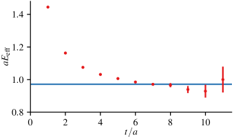
Figure 1: Nucleon effective energy on ensemble A60 with momentum $p_{z}=3(2\pi/L)$. The horizontal line indicates the predicted energy using the nucleon mass from Ref. [50] and the continuum dispersion relation.

On ensemble A60, we performed a dedicated study of excited-state effects by varying the source-sink separation $t_{s}/a$ from 4 to 10. The nucleon effective energy on this ensemble is shown in Fig. 1; although momentum smearing yields a good signal at moderate source-sink separations, the statistical uncertainty still grows rapidly at large separations. Therefore, we use much larger statistics for the larger separations, as given in Table 2.

Matrix elements are obtained from two-point and three-point correlation functions $C_{\text{2pt}}(t_{s})$ and $C_{\text{3pt}}^{\Gamma,z}(\tau,t_{s})$, where $t_{s}$ is the Euclidean time separation between the source and the sink and $\tau$ is the Euclidean time separation between the source and $\mathcal{O}_{\Gamma}(z)$. We consider two estimators for the matrix element $h_{\Gamma}(z)$:

$$\begin{aligned} h_{\Gamma,\text{eff}}^{\text{ratio}}(z;t_{s})&\equiv\frac{C_{\text{3pt}}^{\Gamma,z}(\tfrac{t_{s}}{2},t_{s})}{C_{\text{2pt}}(t_{s})}\\ &=h_{\Gamma}(z)+O\left(e^{-\Delta Et_{s}/2}\right),\\ h_{\Gamma,\text{eff}}^{\text{summ}}(z;t_{s})&\equiv\frac{S_{\Gamma,z}(t_{s}+a)-S_{\Gamma,z}(t_{s})}{a}\\ &=h_{\Gamma}(z)+O\left(e^{-\Delta Et_{s}}\right),\end{aligned}$$ (5)

$$\text{where}\quad S_{\Gamma,z}(t_{s})\equiv a\sum_{\tau/a=1}^{t_{s}/a-1}\frac{C_{\text{3pt}}^{\Gamma,z}(\tau,t_{s})}{C_{\text{2pt}}(t_{s})}$$ (6)

and $\Delta E$ is the energy gap to the lowest excited state.

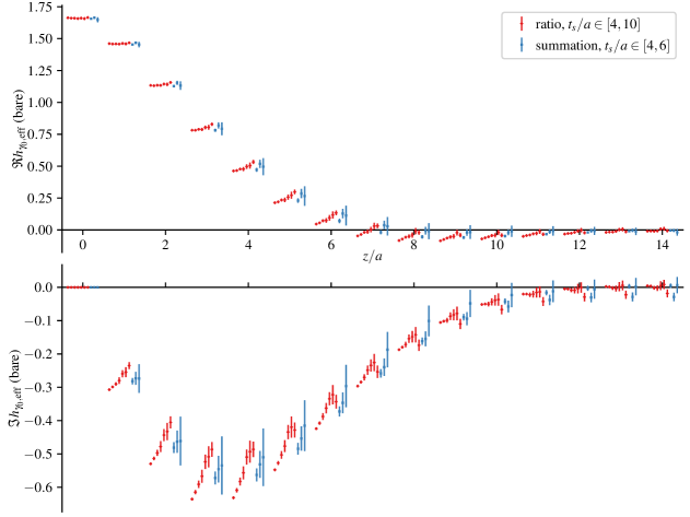
Figure 2: Effective $h_{\gamma_{0}}$ versus $z$: real part (top) and imaginary part (bottom). For each $z$, the ratio-midpoint results are shown using seven source-sink separations, increasing from left to right (red), and the summation-method results are shown using the shortest three source-sink separations (blue).

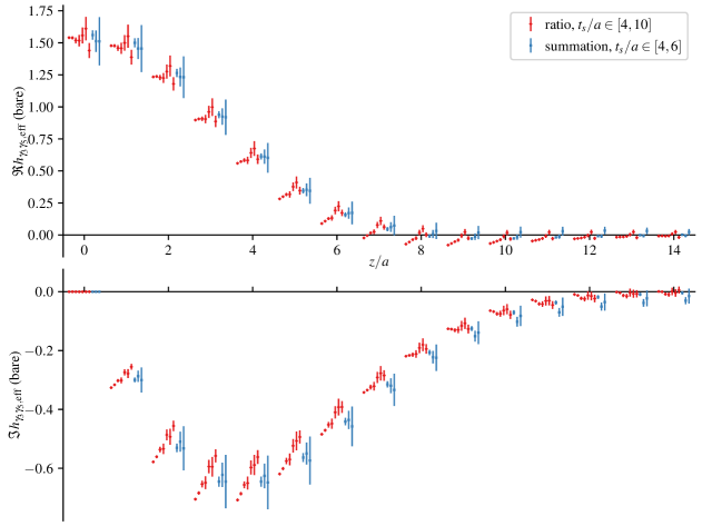
Figure 3: Effective $h_{\gamma_{3}\gamma_{5}}$ versus $z$. See the caption of Fig. 2.

Results are shown for the unpolarized and helicity matrix elements in Figs. 2 and 3. For both observables the excited-state effects are similar. In the real part at small $z$, the dependence on $t_{s}$ is weak, especially for the unpolarized case where $h_{\gamma_{0}}(0)$ is a conserved charge. For $z>6a$, $h_{\text{eff}}$ dips below zero at small $t_{s}$ and this negative part is substantially reduced when $t_{s}$ is increased. In the imaginary part, the negative peak around $z=3a$ is reduced in magnitude when $t_{s}$ is increased.

For most values of $z$, $h_{\text{eff}}^{\text{ratio}}(z)$ with $t_{s}=10a$ is consistent with the value for $t_{s}=8a$ and $9a$ and also with $h_{\text{eff}}^{\text{summ}}(z)$ for $t_{s}=5a$ and $6a$. Therefore we conclude that excited-state effects are reasonably under control using the ratio method with the largest time separation, and we choose to use similar separations for the two other ensembles. However, the analysis in the rest of this paper differs slightly from the excited-state study: instead of simply taking the midpoint $\tau=t_{s}/2$ in $C_{\text{3pt}}^{\Gamma,z}(\tau,t_{s})$, we average over several central values of $\tau$ to reduce the statistical uncertainty. The resulting bare matrix elements for all three ensembles are shown in Fig. 4.

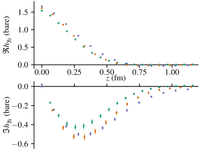
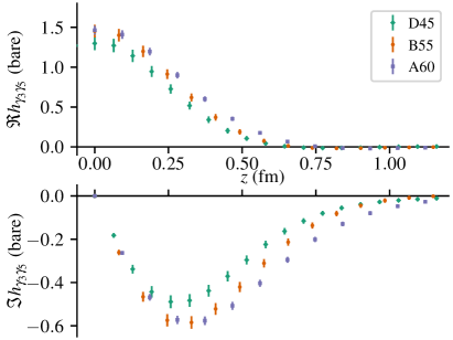
Figure 4: Bare matrix elements: real part (top) and imaginary part (bottom) for the unpolarized (left) and helicity (right) operators.

One risk of studying excited-state effects using just one ensemble is that insufficiently controlled excited-state contributions on the other ensembles could be mistakenly interpreted as discretization effects. To reduce this possibility, $t_{s}$ was chosen to be slightly larger on the two ensembles that lack an excited-states study. Furthermore, our findings in Section IV.3, that accounting for the leading effect of small differences in $p_{z}$ improves the approach to the continuum, and in Section V, that the dependence on $a$ is typically monotonic, are both consistent with discretization effects and not excited-state effects playing the dominant role in this study.

IV Renormalization

Renormalization of the nonlocal operator $\mathcal{O}(z)$ was a stumbling block in rigorously calculating quasi-PDFs and was absent in the earliest lattice QCD calculations [16, 7, 17, 8]. In contrast with local quark bilinears that diverge logarithmically, $\mathcal{O}(z)$ contains a Wilson line that introduces a power divergence. In order to obtain a continuum limit, it is essential that this divergence be removed exactly, meaning that lattice perturbation theory is inadequate. Nonperturbative renormalization prescriptions [9, 19, 45], introduced more than three years after the first lattice quasi-PDF calculations, are necessary.

We employ two different methods for nonperturbative renormalization, both of which involve imposing renormalization conditions on Green’s functions evaluated on Landau-gauge-fixed lattices. For this, we use the $N_{f}=4$ twisted mass ensembles from Ref. [59] listed in Table 3. These have the same action and bare coupling as the ensembles used for computing nucleon matrix elements. However, because of the difficulty in reaching maximal twist with four degenerate light fermions, we instead average over pairs of ensembles with opposite PCAC masses. After renormalizing $\mathcal{O}_{\Gamma}(z)$ in a nonperturbative intermediate scheme, perturbation theory is used to convert first to the $\overline{\text{MS}}$ scheme and then to a modified $\overline{\text{MS}}$ ($\text{M}\overline{\text{MS}}$) scheme [12]. The latter cancels a $\log(z^{2})$ divergence in the $\overline{\text{MS}}$-renormalized matrix element at short distance and enables a matching between quasi-PDF and PDF that conserves charge.

The first method is the whole operator approach, where renormalization conditions are imposed independently on $\mathcal{O}_{\Gamma}(z)$ for each $z$, producing a separate renormalization factor for each $z$. The procedure is very similar to methods commonly used for local quark bilinears, and the nonperturbative intermediate scheme is RI^′-MOM.

The second method is the auxiliary field approach, where the nonlocal operator is rewritten as a pair of local operators in an extended theory. Renormalization conditions are imposed on those local operators and on the action of the extended theory, producing a minimal set of renormalization parameters. The nonperturbative intermediate scheme, RI-xMOM, uses a mixture of momentum space and position space.

When $z=0$, it is a special case where $\mathcal{O}_{\Gamma}(z)$ is a local operator, namely a vector or axial current. For this point, we use the renormalization factor for the corresponding local operator determined in Ref. [59].

In the next two subsections we discuss each method and their sources of systematic uncertainty. In a third subsection, we form a ratio of nucleon matrix elements to cancel the renormalization of $\mathcal{O}_{\Gamma}(z)$ and study the continuum limit of the ratio.

$a\mu$	$\kappa$	$a\mu^{\text{sea}}_{\rm PCAC}$	$aM_{PS}$	lattice size	used in
		$\beta=1.90$, $a=0.0934$ fm
0.0080	0.162689	$+$0.0275(4)	0.280(1)	$24^{3}\times 48$	A
	0.163476	$-$0.0273(2)	0.227(1)
0.0080	0.162876	$+$0.0398(1)	0.279(2)	$24^{3}\times 48$	A,B
	0.163206	$-$0.0390(1)	0.241(1)
		$\beta=1.95$, $a=0.0820$ fm
0.0020	0.160524	$+$0.0363(1)		$24^{3}\times 48$	A,B
	0.161585	$-$0.0363(1)
0.0085	0.160826	$+$0.0191(2)	0.277(2)	$24^{3}\times 48$	A
	0.161229	$-$0.0209(2)	0.259(1)
		$\beta=2.10$, $a=0.0644$ fm
0.0030	0.156042	$+$0.0042(1)	0.127(2)	$32^{3}\times 64$	B
	0.156157	$-$0.0040(1)	0.129(3)
0.0046	0.156017	$+$0.0056(1)	0.150(2)	$32^{3}\times 64$	A
	0.156209	$-$0.0059(1)	0.160(4)
0.0064	0.155983	$+$0.0069(1)	0.171(1)	$32^{3}\times 64$	A
	0.156250	$-$0.0068(1)	0.180(4)

Table 3: Simulation parameters for the $N_{f}=4$ ensembles [59] used in the calculation of the renormalization. The last column indicates which ensembles were used in Sections IV.1 (for the whole-operator renormalization) and IV.2 (for the auxiliary-field renormalization).

IV.1 Whole operator approach and RI^′-MOM scheme

The Rome-Southampton approach [60] and its RI^(′)-MOM schemes are commonly used to determine renormalization factors of local operators. Our prescription for the nonlocal operator $\mathcal{O}_{\Gamma}(z)$ closely follows Refs. [61, 9] and the improvements from Ref. [12] for controlling systematic uncertainties; we refer the reader to those references for a more detailed discussion.

In Landau gauge and in momentum space, we compute the fermion propagator $S_{q}$ [Eq. (13)] and the amputated vertex function $\mathcal{V}_{\mathcal{O}}$, with the operator $\mathcal{O}$ inserted at zero momentum transfer. We impose the conditions

$$\frac{Z^{\text{RI}}_{\cal O}(z,\mu_{0},m_{\pi})}{Z^{\text{RI}}_{q}(\mu_{0},m_{\pi})}\frac{1}{12}{\rm Tr}\left[{\cal V}_{\mathcal{O}}(z,\boldsymbol{p},m_{\pi})\left({\cal V}_{\mathcal{O}}^{\rm Born}(z,\boldsymbol{p})\right)^{-1}\right]\Bigr{|}_{p^{2}{=}\mu_{0}^{2}}{=}1\,,$$ (7)

$$Z^{\text{RI}}_{q}(\mu_{0},m_{\pi})=\frac{1}{12}{\rm Tr}\left[(S_{q}(\boldsymbol{p},m_{\pi}))^{-1}\,S_{q}^{\rm Born}(\boldsymbol{p})\right]\Bigr{|}_{p^{2}=\mu_{0}^{2}}\,,\quad$$ (8)

at each value of $z$, where $X^{\text{Born}}$ is the tree-level value of $X$. As a shorthand, we write $Z_{V}$ for the renormalization of the unpolarized operator $\mathcal{O}_{\gamma_{0}}$ and $Z_{A}$ for the helicity operator $\mathcal{O}_{\gamma_{3}\gamma_{5}}$. We choose the RI^′ renormalization scale, $\mu_{0}$, so that the vertex momentum $\boldsymbol{p}$ has the same components in all spatial directions, that is, $a\boldsymbol{p}=\frac{2\pi}{L_{s}}(n_{t}+\frac{1}{4},n,n,n)$ with integer $n$ and $n_{t}$. More precisely, we choose momenta with $P_{4}\equiv(\sum_{i}p_{i}^{4})/(\sum_{i}p_{i}^{2})^{2}\leq 0.32$, in order to suppress finite-$a$ effects that break rotational symmetry [62, 59].

The renormalization factors are calculated on the $N_{f}=4$ ensembles given in Table 3; these have the same bare coupling $\beta$ as the $N_{f}=2+1+1$ ensembles used for the bare matrix elements. The renormalization procedure can be summarized in the following steps:

1. Calculation of $Z_{\cal O}$ for each ensemble of Table 3, and for several values of the renormalization scale $\mu_{0}$. We use $n_{t}\in[3,9]$, $n\in[2,4]$ for the $24^{3}\times 48$ ensembles, and $n_{t}\in[3,10]$, $n\in[3,5]$ for the $32^{3}\times 64$ ensembles, and restrict to the momenta satisfying $P_{4}\leq 0.3$. The range of values for $(a\mu_{0})^{2}$ is $[1,5]$ and $[1,4]$, for $24^{3}\times 48$ and $32^{3}\times 64$, respectively.

2. Averaging of the two ensembles at opposite $a\mu_{\rm PCAC}^{sea}$ values followed by chiral extrapolation of the form $Z_{0}+(a\mu)Z_{1}$ (or quadratic in $am_{\pi}$) for each lattice spacing. For $\beta=1.90$ we take the average of the four ensembles, as there is only one $a\mu$ value available. For all three $\beta$ values, we find a very mild dependence on the pion mass, similarly to what was found for other ensembles [12].

3. Conversion to the $\overline{\text{MS}}$ scheme and simultaneous evolution to the scale 2 GeV, using the expressions from Ref. [61].

4. Elimination of residual dependence on the RI^′ scale by fitting to extrapolate $(a\mu_{0})^{2}\to 0$. An extensive study on the choice of the renormalization scale and the corresponding systematic uncertainties can be found in Ref. [12]. The optimal fit range for all $\beta$ values is $(a\mu_{0})^{2}\in[1,3]$.

5. Conversion to the $\text{M}\overline{\text{MS}}$ scheme, which is necessary in order to apply a matching formula that satisfies particle number conservation.

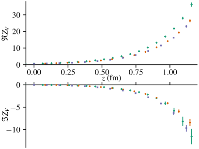
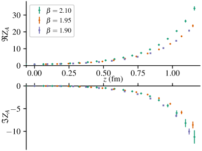
Figure 5: Real part (top) and imaginary part (bottom) of the renormalization factors for the unpolarized (left) and helicity (right) operators in the $\rm M\overline{\text{MS}}$ scheme at 2 GeV, determined using the whole-operator approach via the RI^′-MOM intermediate scheme. Data at $\beta=2.10$, $\beta=1.95$ and $\beta=1.90$ are shown with green diamonds, orange circles, and blue squares, respectively.

The final estimates for renormalization factors are shown in Fig. 5. For the real part, the results with $\beta=1.90$ and 1.95 are very similar, but the latter has a smaller imaginary part. The finest lattice spacing, $\beta=2.10$, has a larger real part. The renormalized matrix elements from the three lattice spacings are shown in Fig. 11 and their approach to the continuum limit is discussed in Section V.1.

IV.2 Auxiliary field approach and RI-xMOM scheme

The auxiliary field approach [63, 64, 65, 45] introduces a new field $\zeta(z)$ whose propagator is a Wilson line along the $\boldsymbol{\hat{z}}$ direction. This allows the nonlocal operator in QCD to be represented using the local operator $\phi\equiv\bar{\zeta}\psi$ in the extended theory:

$$\mathcal{O}_{\Gamma}(\boldsymbol{x},z)=\left\langle\bar{\phi}(\boldsymbol{x}+z\boldsymbol{\hat{z}})\Gamma\tau_{3}\phi(\boldsymbol{x})\right\rangle_{\zeta}.$$ (9)

The problem becomes that of renormalizing the action for $\zeta$ and the composite operator $\phi$; one finds that three parameters are sufficient to renormalize all operators $\mathcal{O}_{\Gamma}(z)$ [45]:

$$\mathcal{O}_{\Gamma}^{R}(z)=Z_{\phi}^{2}e^{-m|z|}\left[\mathcal{O}_{\Gamma}(z)+\operatorname{sgn}(z)r_{\text{mix}}\mathcal{O}_{\{\gamma_{z},\Gamma\}}+r_{\text{mix}}^{2}\mathcal{O}_{\gamma_{z}\Gamma\gamma_{z}}\right],$$ (10)

where $m$ is linearly divergent, $Z_{\phi}$ is logarithmically divergent, and $r_{\text{mix}}$ is finite and associated with chiral symmetry breaking on the lattice. For our choices of $\Gamma$, the anticommutator vanishes and the expression simplifies to

$$\mathcal{O}_{\Gamma}^{R}(z)=Z_{\phi}^{2}(1-r_{\text{mix}}^{2})e^{-m|z|}\mathcal{O}_{\Gamma}(z).$$ (11)

We follow the approach in Refs. [45, 47] to determine $m$ and $Z_{\phi}^{2}(1-r_{\text{mix}}^{2})$, using the RI-xMOM intermediate scheme and converting to $\overline{\text{MS}}$. Calculations are performed using the most chiral $N_{f}=4$ twisted mass ensembles from Ref. [59], averaging over pairs of ensembles with opposite PCAC masses rather than directly working at maximal twist. In addition to the operator with stout-smeared links used for the bare nucleon matrix elements, we also employ unsmeared links, which are expected to have reduced discretization effects, in some intermediate steps. After fixing to Landau gauge, we compute the position-space $\zeta$ propagator

$$S_{\zeta}(z)\equiv\langle\zeta(z\boldsymbol{\hat{z}})\bar{\zeta}(\boldsymbol{0})\rangle_{\text{QCD}+\zeta}=\langle W(z\boldsymbol{\hat{z}},\boldsymbol{0})\rangle_{\text{QCD}};$$ (12)

the momentum-space quark propagator,

$$S_{q}(\boldsymbol{p})\equiv\int d^{4}\boldsymbol{x}e^{-i\boldsymbol{p}\cdot\boldsymbol{x}}\langle\chi(\boldsymbol{x})\bar{\chi}(\boldsymbol{0})\rangle,$$ (13)

where $\chi$ is a quark field in the twisted basis; and the mixed-space Green’s function for $\phi$,

$$G_{\phi}(z,\boldsymbol{p})\equiv\int d^{4}xe^{i\boldsymbol{p}\cdot\boldsymbol{x}}\langle\zeta(z\boldsymbol{\hat{z}})\phi(\boldsymbol{0})\bar{\chi}(\boldsymbol{x})\rangle_{\text{QCD}+\zeta}.$$ (14)

These renormalize as

$$S_{\zeta}^{R}(z) =Z_{\zeta}e^{-m|z|}S_{\zeta}(z),$$ (15)

$$S_{q}^{R}(\boldsymbol{p}) =Z_{q}S_{q}(\boldsymbol{p}),$$ (16)

$$G_{\phi}^{R}(z,\boldsymbol{p}) =Z_{\phi}\sqrt{Z_{\zeta}Z_{q}}e^{-m|z|}G_{\phi}(z,\boldsymbol{p}).$$ (17)

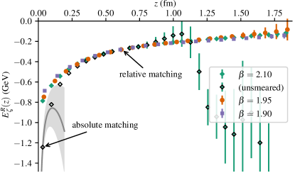
Figure 6: Renormalized $E_{\zeta}(z)$ versus $z$. Filled blue squares, orange circles, and green diamonds show the data with stout-smeared links on the coarse, medium, and fine lattice spacings, respectively. Diamonds with black outlines show the data on the fine lattice spacing without smearing. Note that a hypercubic rotation has been used to orient the Wilson line in the temporal direction to reduce finite-volume effects at large $z$. The curve shows the perturbative result based on the analytic three-loop calculation [66, 67], the analytic partial four-loop calculations [68, 69, 69, 70, 71, 72, 73, 74], and the numerical full four-loop calculation [72]; its error band indicates the size of the $O(\alpha_{s}^{4})$ contribution.

To fix $m$, we evaluate the effective energy of the $\zeta$ propagator,

$$E_{\zeta}(z)\equiv-\frac{d}{dz}\log\operatorname{Tr}S_{\zeta}(z),$$ (18)

which is renormalized by adding $m$. We use the nearest-neighbor lattice derivative. The relative matching among the three lattice spacings is done at $z\approx 0.61$ fm. The absolute value of $m$ is determined using unsmeared links on the finest lattice spacing, which is expected to produce the smallest discretization effects, and matching to the perturbative results for the static quark propagator known to $O(\alpha_{s}^{4})$ [47, 66, 67, 68, 69, 69, 70, 71, 72, 73, 74]. The results are shown in Fig. 6. Except at short distance where discretization effects are significant, the three lattice spacings are in good agreement for the renormalized effective energy.

The other renormalization factors are determined using conditions designed to eliminate dependence on $m$:

$$\frac{-i}{12p^{2}Z_{q}^{\text{RI}}}\operatorname{Tr}\left[S_{q}^{-1}(\boldsymbol{p})\not{\boldsymbol{p}}\right]=1,$$ (19)

$$\frac{Z_{\zeta}^{\text{RI}}}{3}\frac{[\operatorname{Tr}S_{\zeta}(z)]^{2}}{\operatorname{Tr}S_{\zeta}(2z)}=1,$$ (20)

$$\frac{1}{12}\frac{Z_{\phi}^{\text{RI}}(1\pm r_{\text{mix}})}{\sqrt{Z_{\zeta}^{\text{RI}}Z_{q}^{\text{RI}}}}\Re\operatorname{Tr}\left[(1\pm\gamma_{z})S_{\zeta}^{-1}(z)G_{\phi}(z,\boldsymbol{p})S_{q}^{-1}(\boldsymbol{p})\right]=1.$$ (21)

These are evaluated at the scale $\mu^{2}=p^{2}$, choosing $\boldsymbol{p}=p_{z}\boldsymbol{\hat{z}}$. This defines a family of renormalization schemes that depend on the dimensionless quantity $y\equiv p_{z}z$. From the above, we extract the relevant overall renormalization factor, $Z_{\phi}^{2}(1-r_{\text{mix}}^{2})$, at fixed kinematics. We then convert $Z_{\phi}$ to the $\overline{\text{MS}}$ scheme using the one-loop expression from Refs. [45, 47] and evolve to the scale 2 GeV using the two-loop anomalous dimension of the static-light current [75, 76].

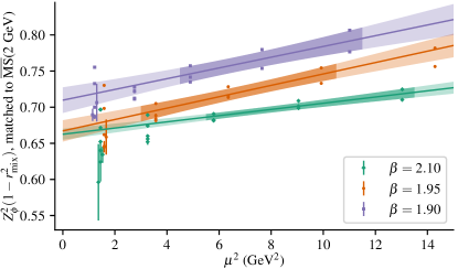
Figure 7: Renormalization factor $Z_{\phi}^{2}(1-r_{\text{mix}}^{2})$ determined using unsmeared links in the RI-xMOM scheme, matched to $\overline{\text{MS}}$, and evolved to scale 2 GeV. A hypercubic rotation has been used to orient the Wilson line and the quark momentum in the temporal direction. The multiple points at the same $\mu^{2}$ have different values of the RI-xMOM scheme parameter $y$. The lines with error bands give the extrapolation to $a^{2}\mu^{2}=0$ and the darker part of each error band indicates the fit range.

The determination of $Z_{\phi}^{2}(1-r_{\text{mix}}^{2})$ is shown in Fig. 7. As this is done at relatively high scales where the perturbative matching and evolution are applicable, we do this using unsmeared gauge links. Except at low $\mu^{2}$, the statistical uncertainty is negligible compared with systematics. At each $\mu^{2}$, we estimate the latter such that the spread of results for different scheme parameters $y$ is covered. For each lattice spacing, we extrapolate $a^{2}\mu^{2}$ to zero assuming a linear dependence; the systematic uncertainty is propagated assuming a 50% correlation between every pair of points. Following the approach used in Ref. [45], we match between unsmeared and smeared links in the infrared regime at large $z$ and small $p^{2}$.

$\beta$	$am$	$Z_{\phi}^{2}(1-r_{\text{mix}}^{2})$
1.90	$-0.392(1)(57)$	0.986(25)
1.95	$-0.373(1)(50)$	0.908(20)
2.10	$-0.305(1)(37)$	0.907(11)

Table 4: Renormalization parameters from the auxiliary-field approach, determined via the RI-xMOM intermediate scheme. The second uncertainty for the auxiliary field mass comes from the absolute matching onto perturbation theory and is fully correlated across the three ensembles.

Final parameters for operators with stout-smeared links are given in Table 4. The large uncertainty for the mass parameter is caused by the absolute matching onto perturbation theory. At each $z$, this absolute matching produces an overall factor applied to $h_{\Gamma}(z)$ at all three lattice spacings. Therefore it can be ignored when studying the approach to the continuum limit. However, this uncertainty must be included when comparing continuum-limit results against other renormalization approaches.

An additional perturbative conversion [12] yields results in the $\text{M}\overline{\text{MS}}$ scheme; this cancels a $\log(z^{2})$ divergence in the $\overline{\text{MS}}$-renormalized matrix element at short distance. However, this conversion has only been computed at one-loop order, meaning that the cancellation may be inexact and some part of the divergence may still remain. The renormalized nucleon matrix elements for the three lattice spacings are shown in Fig. 10.

IV.3 Ratio with zero-momentum matrix element

Ensemble	$N_{\text{conf}}$	$N_{\text{samp}}$
A60	79	316
B55	54	216
D45	65	260

Table 5: Statistics used for the nucleon matrix elements at zero momentum.

The simplest way to cancel ultraviolet divergences is to compute matrix elements of the same operator in different hadronic states and then take their ratio. Here we choose to take the ratio of matrix elements in a nucleon at nonzero momentum (i.e. those used throughout this paper) with the same in a nucleon at rest,

$$R_{\Gamma}(p_{z},z)\equiv\frac{h_{\Gamma}(p_{z},z;\mu)}{h_{\Gamma}(0,z;\mu)}.$$ (22)

As the signal-to-noise problem is much milder in a nucleon at rest, this requires a relatively inexpensive additional calculation: see Table 5.

This ratio is similar to the reduced Ioffe-time distribution used in the pseudo-PDF approach for parton distributions [77]. Although it is a different observable than the $\text{M}\overline{\text{MS}}$-renormalized matrix elements used for quasi-PDFs, it provides the opportunity to study the approach to the continuum limit in a clean, controlled setting. As such, this section can be seen as a preview of the continuum extrapolations of the renormalized matrix element $h_{\Gamma}$ in Section V.1.

We consider variations of the continuum extrapolation in two different ways. First: precisely which points should be used to obtain $R_{\Gamma}(p_{z},z)$ at zero lattice spacing? One option is to ignore small differences in $p_{z}$ among the three ensembles, interpolate the lattice data to a common value of $z$ in physical units, and then perform the extrapolation. Alternatively, noting that parameter $x$ of quasi-PDFs is Fourier-conjugate to the product $zp_{z}$, we can choose to interpolate to a common value of $zp_{z}$ before extrapolating; this could be more reliable because it accounts at leading order for the small differences in $p_{z}$.

Second: what fit form should be used? As we have three lattice spacings, we restrict ourselves to two-parameter fits. At $z=0$, the operator $\mathcal{O}$ is local, namely a vector or axial current; since we work at maximal twist, this calculation benefits from automatic $O(a)$ improvement [78, 79] and we extrapolate using an affine function of $a^{2}$. For $z\neq 0$ (i.e. for the bulk of our data), $\mathcal{O}$ is nonlocal and there can be $O(a)$ contributions that are not eliminated by automatic improvement [47]. In practice, it is not clear whether we are in the regime where $O(a)$ contributions dominate; therefore, we extrapolate using both affine functions of $a$ and of $a^{2}$.

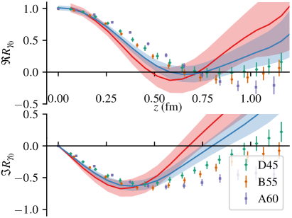
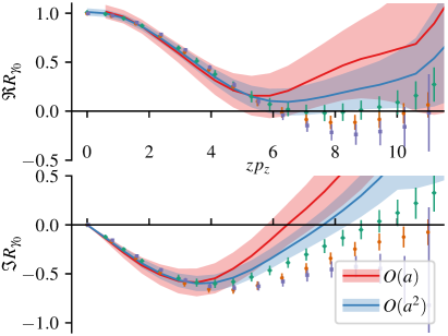
Figure 8: Real part (top) and imaginary part (bottom) of the ratio of unpolarized matrix elements $R_{\gamma_{0}}$ versus $z$ in physical units (left) and versus $zp_{z}$ (right). The curves with error bands depict the results from the continuum extrapolations assuming leading artifacts linear in $a$ (red) and quadratic in $a$ (blue).

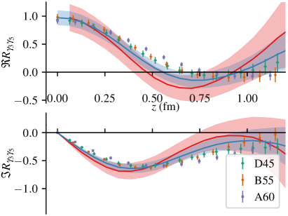
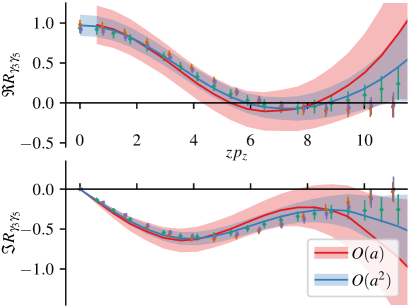
Figure 9: Ratio of helicity matrix elements $R_{\gamma_{3}\gamma_{5}}$. See the caption of Fig. 8.

The ratio data and their extrapolations are shown in Figs. 8 and 9. When plotted versus $z$ in physical units, clear discrepancies between the three ensembles are visible and for most of the parameter space, the lattice data from the coarsest ensemble are more than one standard deviation away from the extrapolations. These discrepancies are reduced when plotting the data versus $zp_{z}$, although they remain significant for the unpolarized data at large $z$.

From this study, it appears that performing the extrapolation at fixed values of $zp_{z}$ is a better approach. For the unpolarized matrix elements with $zp_{z}<5$ and for the helicity matrix elements, lattice artifacts have a modest effect and are well under control, with the $O(a)$ and $O(a^{2})$ extrapolations in good agreement. For the unpolarized matrix elements with $zp_{z}>5$, there is a stronger dependence on $a$ and worse agreement between the two extrapolations; this suggests that at longer distances the lattice artifacts are less well controlled.

V Continuum limit

V.1 Renormalized matrix elements

Based on our study of the ratios of matrix elements in the previous section, we choose to linearly interpolate our $\text{M}\overline{\text{MS}}$-scheme renormalized matrix elements to common values of $zp_{z}$ and then perform continuum extrapolations at each interpolated point. We again extrapolate in two ways, assuming lattice artifacts are either linear or quadratic in the lattice spacing.

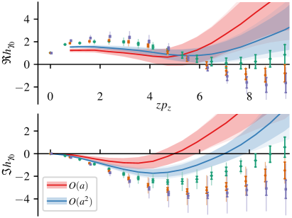
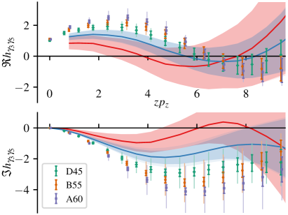
Figure 10: Matrix elements renormalized using the auxiliary field approach via matching from the intermediate RI-xMOM scheme: real part (top) and imaginary part (bottom) of the unpolarized (left) and helicity (right) matrix elements, converted to the $\text{M}\overline{\text{MS}}$ scheme at scale 2 GeV. The curves with error bands depict the results from the continuum extrapolations assuming leading artifacts linear in $a$ (red) and quadratic in $a$ (blue). The outer error bars (without endcaps) and outer error bands include the uncertainty from the absolute matching of the auxiliary field mass onto perturbation theory, which is fully correlated among the three ensembles.

Figure 10 shows the matrix elements renormalized using the auxiliary field approach and their continuum extrapolations. For most values of $zp_{z}$, there is a large dependence on the lattice spacing and the extrapolated values are far from those of the individual ensembles. The extrapolations tend to reduce the magnitude of the matrix element, except for the unpolarized case at large $zp_{z}$, where both the real and imaginary parts are positive and growing. For the unpolarized matrix element, the $O(a)$ and $O(a^{2})$ extrapolations are not in good agreement, particularly in the real part at small $zp_{z}$ and the imaginary part at medium $zp_{z}$.

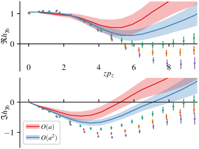
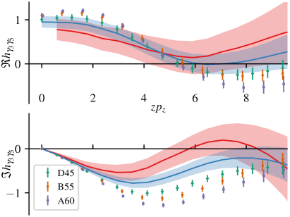
Figure 11: Matrix elements renormalized using the whole operator approach via matching from the intermediate RI^′-MOM scheme: real part (top) and imaginary part (bottom) of the unpolarized (left) and helicity (right) matrix elements, converted to the $\text{M}\overline{\text{MS}}$ scheme at scale 2 GeV. The curves with error bands depict the results from the continuum extrapolations assuming leading artifacts linear in $a$ (red) and quadratic in $a$ (blue).

Matrix elements renormalized using the whole-operator approach are shown in Fig. 11, along with their continuum extrapolations. Qualitatively, the picture is similar to the auxiliary-field renormalization approach, except that at small $zp_{z}$, the real part of the matrix elements from the three lattice spacings are in better agreement, producing a milder effect from the continuum extrapolation and a better agreement between the two extrapolations. The latter is especially true for the unpolarized matrix element. Details of these continuum extrapolations for selected values of $zp_{z}$ are shown in Figs. 12 and 13. Clearly, our lever arm in $a$ is limited, which makes it difficult to detect a preference for either of the two fits; this also produces a large uncertainty for the $O(a)$ extrapolations.

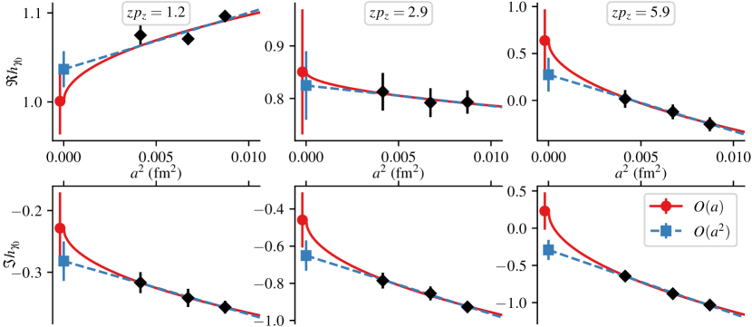
Figure 12: Continuum extrapolation of unpolarized matrix elements renormalized using the whole operator approach: real part (top) and imaginary part (bottom), versus $a^{2}$. Results are shown for $zp_{z}=1.2$ (left), 2.9 (center), and 5.9 (right). Black diamonds show the data from ensemble D45 and interpolated data from ensembles B55 and A60. The solid red curve and red circle show the $O(a)$ extrapolation; the dashed blue line and blue square show the $O(a^{2})$ extrapolation.

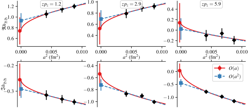
Figure 13: Continuum extrapolation of helicity matrix elements renormalized using the whole operator approach. See the caption of Fig. 12.

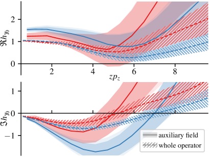
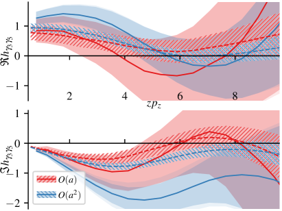
Figure 14: Comparison of continuum-extrapolated matrix elements: real part (top) and imaginary part (bottom) of the unpolarized (left) and helicity (right) matrix elements, in the $\text{M}\overline{\text{MS}}$ scheme at scale 2 GeV. Solid bands show data using the auxiliary field approach via the RI-xMOM intermediate scheme and hatched bands show results using the whole-operator approach via the RI^′-MOM intermediate scheme.

Results from the two renormalization approaches are compared in Fig. 14. The whole operator approach tends to produce a smaller central value and a smaller uncertainty than the auxiliary field method. For the imaginary part of the matrix elements, the $O(a^{2})$ auxiliary-field extrapolation is in significant disagreement with both of the whole-operator extrapolations. In contrast, the $O(a)$ result using the auxiliary field method is largely compatible with both whole-operator extrapolations, for low to medium values of $zp_{z}$. This suggests that there may be significant $O(a)$ lattice artifacts in the determination of the auxiliary field renormalization parameters and that it is necessary to account for them when taking the continuum limit.

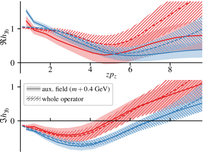
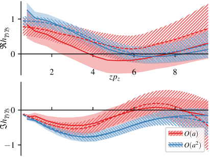
Figure 15: Comparison of continuum-extrapolated matrix elements, after reducing the magnitude of the auxiliary-field mass renormalization by 0.4 GeV. See the caption of Fig. 14.

Since renormalization in the auxiliary field approach is determined by just two parameters, one might ask whether there exist parameters that produce results compatible with the whole operator method. Figure 15 shows the effect of reducing the magnitude of the auxiliary-field mass renormalization parameter by $\delta m=0.4$ GeV. Although this adjustment is hard to justify from the analysis in Section IV.2, in Ref. [58] it was shown that its effect on quasi-PDFs is suppressed by the factor $\delta m/p_{z}$ at large momentum. This change produces good agreement for the imaginary part of the matrix elements. However, some discrepancies remain for the real part, particularly in the unpolarized case at small $zp_{z}$, where the slope of the auxiliary-field result is considerably steeper than the whole-operator data.

In the rest of this paper where we examine the effect on parton distributions, we will focus on the more precise data renormalized using the whole-operator method. However, we will continue to compare $O(a)$ and $O(a^{2})$ extrapolations since they are not in complete agreement and we have no a priori reason to prefer one over the other.

V.1.1 Comparison with phenomenology

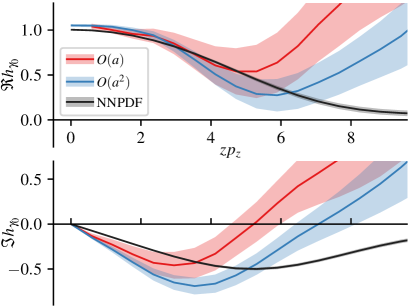
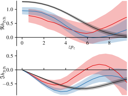
Figure 16: Unpolarized (left) and helicity (right) matrix elements from continuum extrapolation of lattice data renormalized using the whole operator approach via the RI^′-MOM intermediate scheme (blue, red) and from the inverse Fourier transform of the quasi-PDFs obtained by applying inverse matching to phenomenological PDFs from NNPDF [80, 81] (dark gray). Note that in the lattice calculation, the pion mass is much larger than in nature, so that exact agreement should not be expected.

Before transforming the position-space matrix elements to obtain PDFs and comparing directly with phenomenology, we perform the reverse exercise. Starting with phenomenological parton distributions determined by NNPDF [80, 81], we invert the matching and the Fourier transform to determine the position-space matrix elements that yield those PDFs, up to higher-order corrections in the matching. Figure 16 compares this with the continuum-extrapolated lattice matrix elements. Full agreement cannot be expected, since the lattice calculation was done at a heavy pion mass and other systematics such as the dependence on $p_{z}$ and finite-volume effects have not been included in this study.

The real part of the unpolarized matrix elements show reasonable agreement for $zp_{z}<5$; in the same range, the helicity matrix elements from the lattice lie below those from phenomenology. The helicity case can be partly understood by recalling that at heavy pion masses, the nucleon axial charge (i.e. the helicity matrix element at $z=0$) lies below its physical value. At short distances, the imaginary parts of the lattice data have larger (more negative) slopes than phenomenology; the $O(a)$ extrapolations are consistent with the latter at the $1\sigma$ level whereas the $O(a^{2})$ extrapolations are not. At nonzero lattice spacing, the slope is even larger and in worse agreement with NNPDF, so that the continuum extrapolation produces results that lie closer to phenomenology.

At larger values of $zp_{z}$, there is a qualitative difference: the phenomenological curves tend steadily toward zero, whereas the lattice data do not. This is especially true for the unpolarized lattice matrix elements, of which both the real and imaginary parts are positive and increasing at large distances. At the coarsest lattice spacing, the lattice data lie well below zero (see Fig. 11), so it appears that the continuum extrapolation may be an overcorrection. Another way to characterize the imaginary part is via the position of the minimum of the curve: in the lattice data, it lies at a shorter distance than in phenomenology. This is consistent with the general expectation that correlation functions are shorter ranged at heavier pion masses.

V.2 Parton distributions

In this section, we present the main results of this paper, namely the effect of the continuum extrapolation on PDFs. However, we first discuss another source of systematic uncertainty: how to perform the Fourier transform in the definition of the quasi-PDF using a finite set of position-space data. We illustrate this using data on the finest ensemble, D45. Next, we perform the continuum extrapolation at fixed $x$, using the PDFs determined on each ensemble, and compare the result with the PDF determined from the continuum-limit matrix elements obtained in the previous section. Finally, we compare our continuum-limit PDFs with phenomenology.

V.2.1 Reconstruction techniques

As given in Eq. (3), the quasi-PDF $\tilde{q}(x)$ is obtained from a Fourier transform (FT) of the renormalized matrix elements $h(z)$. In practice, we obtain $h(z)$ at intervals of the lattice spacing, i.e. $z/a\in\mathbb{Z}$. It is also necessary to truncate the FT at $|z|\leq z_{\text{max}}$, both because of the finite lattice size, which imposes $z_{\text{max}}\lesssim L/2$, and because of growing statistical uncertainty at large $|z|$. Together, these have the effect of replacing the continuous FT by a truncated discrete FT (DFT):

$$\frac{p_{z}}{2\pi}\int_{-\infty}^{\infty}dz\,e^{-ixp_{z}z}\rightarrow\frac{p_{z}}{2\pi}a\sum_{z/a=-z_{\text{max}}/a}^{z_{\text{max}}/a}e^{-ixp_{z}z}.$$ (23)

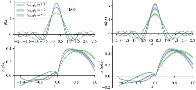
Figure 17: Unpolarized (left) and helicity (right) quasi-PDFs (top panels) and PDFs (bottom panels) of the D45 ensemble for different values of the cutoff $z_{\text{max}}$. The curves with cutoff at $z_{\text{max}}p_{z}=\{3.5,4.7,5.9\}$ are depicted in green, blue and gray.

The discrete sampling makes the result formally periodic, so that it must be cut off at $|x|\leq\pi/(ap_{z})$, which is at least 4 in our setup. The truncation introduces an additional systematic uncertainty [12], as shown using ensemble D45 in Fig. 17 for quasi-PDFs and PDFs. The latter are obtained by applying the matching procedure and nucleon mass corrections [17]. For the quasi-PDF, the effect of truncation is that one obtains a convolution of the desired result:

$$\tilde{q}^{\text{DFT}}(x) =\frac{ap_{z}}{2\pi}\int_{-\pi/(ap_{z})}^{\pi/(ap_{z})}dx^{\prime}\,\frac{\sin((x-x^{\prime})p_{z}(z_{\text{max}}+a/2))}{\sin((x-x^{\prime})p_{z}a/2)}\tilde{q}(x^{\prime})$$ (24)

$$\xlongrightarrow{a\to 0}\frac{1}{\pi}\int_{-\infty}^{\infty}dx^{\prime}\,\frac{\sin((x-x^{\prime})z_{\text{max}}p_{z})}{(x-x^{\prime})}\tilde{q}(x^{\prime}),$$

so that any features narrower in $x$ than $(z_{\text{max}}p_{z})^{-1}$ are smeared out. This is clearly visible in Fig. 17, where smaller values of $z_{\text{max}}p_{z}$ are associated with broader quasi-distributions. The effect is reduced after applying the matching to obtain PDFs: results with $z_{\text{max}}p_{z}=4.7$ and 5.9 are very similar. However, for $z_{\text{max}}p_{z}=3.5$, both the unpolarized and helicity PDFs have qualitatively quite different behaviour, with a higher value for $x$ between roughly $-0.7$ and $-0.1$ and a larger slope for $x$ less than $-0.3$ as well as a smaller slope at small positive $x$ and a peak at larger $x$ in the positive region.

Since the Fourier transform introduces a systematic uncertainty, we supplement the naïve truncated FT with more sophisticated reconstruction techniques [82, 83]. In these approaches, obtaining the Fourier transform from a finite number of data points is seen as an ill-defined inverse problem. Its solution is not unique and one approach is to use explicit models for the shape of the (quasi-)PDF. By contrast, we choose to use two approaches that do not contain an explicit model: the Backus-Gilbert method, first applied for PDFs calculations in [82] and the Bayes-Gauss-Fourier Transform (BGFT) [83]. These two procedures address the reconstruction problem as follows.

Backus-Gilbert (BG)

The inverse problem is obtained by inverting Eq. (3) to write the real and imaginary parts of the unpolarized matrix element in terms of the quasi-PDF:

$$\Re h_{\gamma_{0}}(p_{z},z;\mu) =\int_{0}^{\infty}dx\,\cos(xp_{z}z)\,\tilde{q}_{+}(x,p_{z};\mu),$$ (25)

$$\Im h_{\gamma_{0}}(p_{z},z;\mu) =\int_{0}^{\infty}dx\,\sin(xp_{z}z)\,\tilde{q}_{-}(x,p_{z};\mu),$$

where for $x\geq 0$, $\tilde{q}_{\pm}(x)=\tilde{q}(x)\pm\tilde{q}(-x)$, and likewise for the helicity case. The reconstruction is applied independently to $\tilde{q}_{+}$ and $\tilde{q}_{-}$, so for brevity we describe the procedure applied to $\tilde{q}_{+}$. We also omit the labels $p_{z}$ and $\mu$. For each $x$, the solution is assumed to be a linear combination of the finite set of lattice data:

$$\tilde{q}_{+}^{\text{BG}}(x)=\sum_{z/a=0}^{z_{\text{max}}/a}\textbf{a}_{+}(x,z)\Re h_{\gamma_{0}}(z),$$ (26)

where $\textbf{a}_{+}$ can be understood as an approximation to the inverse of the Fourier transform in Eq. (25). The accuracy of this approximation is governed by the function

$$\Delta_{+}(x,x^{\prime})=\sum_{z/a=0}^{z_{\text{max}}/a}\textbf{a}_{+}(x,z)\cos(x^{\prime}p_{z}z)$$ (27)

that approximates $\delta(x-x^{\prime})$. Specifically, the result is an integral over the quasi-PDF:

$$\tilde{q}_{+}^{\text{BG}}(x)=\int_{0}^{\infty}dx^{\prime}\,\Delta_{+}(x,x^{\prime})\tilde{q}_{+}(x^{\prime}).$$ (28)

The function $\textbf{a}_{+}$ is determined by the Backus-Gilbert procedure [84], which minimizes the width of $\Delta_{+}(x,x^{\prime})$. For more details, see Refs. [82, 40].

Bayes-Gauss-Fourier Transform (BGFT)

Rather than directly reconstructing $\tilde{q}$ from the lattice data, this procedure reconstructs a continuous form of the position-space matrix elements for all values of $z$:

$$h(z),\,z/a\in\{0,\pm 1,\pm 2,\dots,\pm z_{\text{max}}/a\}\longrightarrow h^{\text{GPR}}(z),\,z\in\mathbb{R}.$$ (29)

For this, we apply a nonparametric regression technique, based on Bayesian inference, called Gaussian process regression (GPR) [85]. This allows us to incorporate into the prior distribution the asymptotic behavior of the matrix elements (expected to decay to zero), as well as their smoothness properties. The result is continuous, defined for all real $z$, and has a Fourier transform computable in closed form. Taking the FT of $h^{\text{GPR}}(z)$, we refer to the result as $\tilde{q}^{\text{BGFT}}(x)$. More details are given in Ref. [83].

Figure 18: Comparison of quasi-PDFs (top panels) and PDFs (bottom panels) of the D45 ensemble obtained from Bayes-Gauss-Fourier Transform (BGFT), Backus-Gilbert (BG) and discrete FT (DFT) for the unpolarized (left) and helicity (right).

In Fig. 18, we compare results from the truncated discrete Fourier transform, Eq. (23), and the BG and BGFT reconstruction methods described above, again using ensemble D45 as our reference data set. For a fair comparison, in all cases we use $z_{\text{max}}p_{z}=4.7$. We begin by discussing the quasi-PDFs (upper two panels). The most striking difference is that the Backus-Gilbert result has a discontinuity at $x=0$ that is not present in the other results. This is because $\tilde{q}_{-}^{\text{BG}}(x)$ is not constrained to vanish at $x=0$. Such a discontinuity could occur if $\Im h(z)$ has a slowly decaying tail $\sim 1/z$. For $x$ between $-0.5$ and $1.0$, the DFT and BGFT results are similar, although the BGFT distribution is slightly narrower. For larger values of $|x|$, the DFT produces stronger oscillations, which are suppressed by the BGFT. The BG result is the outlier, being considerably smaller at small negative $x$ and also having a smaller dip below zero.

We next discuss the physically relevant parton distributions, obtained after matching and nucleon mass corrections (lower two panels). For most values of $x$, the DFT and BGFT method produce very similar results, although for BGFT the the dip below zero in the antiquark region occurs at smaller negative $x$ and the magnitude is smaller at $x=-1$ and $+1$. Again, the BG result is somewhat different: in the antiquark region at small negative $x$, the small positive bump is gone and the result is either consistent with zero (unpolarized) or slightly negative (helicity). This discrepancy at small $x$ may be associated with a lack of data for the matrix element at large $|z|$; better data or a more rigorous understanding of the large-$|z|$ behavior could help to improve this situation. In the quark region for $x$ greater than about 0.5, the BG result has a much weaker downward trend than the other two methods. Given that the DFT produces a result not substantially different from BGFT, we exclude the DFT from further analyses presented in the next sections.

V.2.2 Continuum extrapolation

In what follows, we compare the distributions at finite lattice spacings with continuum extrapolations. In the reconstruction of the quasi-PDFs we use the lattice data with $|zp_{z}|\leq z_{\text{max}}p_{z}=4.7$, at which point either the real part or the imaginary part of the continuum matrix element is compatible with zero, as shown in Fig. 11. Moreover, we estimate the systematic uncertainty from this choice of the cutoff by varying $z_{\text{max}}$:

$$\varepsilon_{\rm cutoff}(x)=\frac{|q_{z_{\text{max}}p_{z}=5.9}(x)-q_{z_{\text{max}}p_{z}=3.5}(x)|}{2}.$$ (30)

Finally, we estimate the combined uncertainty as the quadrature sum of $\varepsilon_{\rm cutoff}(x)$ and the statistical uncertainty.

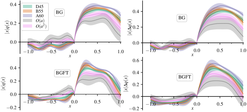
Figure 19: Matched unpolarized (left) and helicity (right) PDFs obtained using the gauge ensembles A60 (blue), B55 (orange), D45 (green), whose lattice spacings are reported in Table 1. The PDF in the continuum, after $O(a)$ extrapolation (gray) and $O(a^{2})$ extrapolation (pink), is also shown.

One approach for obtaining continuum-limit PDFs is to take the PDF determined on each ensemble and then perform an $O(a)$ or $O(a^{2})$ extrapolation of the data at each $x$. This is shown in Fig. 19, for both unpolarized and helicity PDFs determined using the BG and BGFT methods. In the quark region with $x$ between roughly 0 and 0.7, the PDFs decrease monotonically with the lattice spacing; at larger $x$, the D45 data (with the finest lattice spacing) move relatively upward to lie between those of the other two ensembles. For all $x>0$, the $O(a^{2})$ extrapolation lies below all of the individual lattice spacings and the $O(a)$ extrapolation is even lower. Using the BGFT approach, both of the extrapolations are consistent with the expected value of zero at $x=1$, whereas for BG, this is true only of the $O(a)$ extrapolation. In the antiquark region, the extrapolated results lie above the PDFs determined at finite lattice spacing, except for the BGFT unpolarized distribution near $x=-1$. This produces a more prominent positive region at small negative $x$, particularly in the unpolarized case. At larger negative $x$, the extrapolations are generally closer to zero.

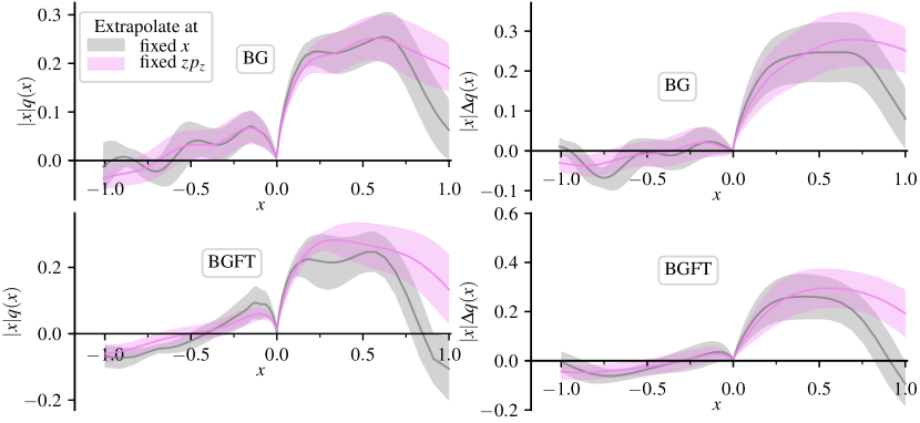
Figure 20: Comparison between the results for the unpolarized (left) and helicity (right) PDFs in the continuum limit obtained with the $O(a)$ extrapolation at fixed $x$ (gray; see Fig. 19) and at fixed $zp_{z}$ (pink, based on the continuum-limit data in Fig. 11). The distributions has been obtained using the BG (top panels) and BGFT (bottom panels) reconstruction techniques.

Another approach is to obtain PDFs from the continuum limit of $h(z)$ as determined in Section V.1 by extrapolating data at fixed $zp_{z}$. By changing the order in which the continuum limit and the combination of the Fourier transform and PDF matching are performed, we obtain results affected by different systematic effects. The comparison of the $O(a)$ extrapolations from both approaches is shown in Fig. 20. They are consistent within uncertainties, except near $x=1$, where the fixed-$x$ extrapolation is in all cases lower than the fixed-$zp_{z}$ extrapolation and only the former is consistent with zero at $x=1$.

For comparing with phenomenology in the next section, we take the fixed-$x$ extrapolation as our central value and add an additional systematic uncertainty in quadrature, namely half the difference with the fixed-$zp_{z}$ extrapolation.

V.2.3 Comparison with phenomenology

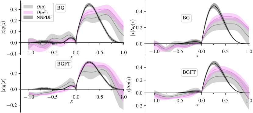
Figure 21: Unpolarized (left) and helicity (right) distributions in the continuum, using BG (top) and BGFT (bottom) methods. $O(a)$ and $O(a^{2})$ extrapolations are shown in gray and pink, respectively. PDFs extracted through global fits from the releases NNPDF [80, 81] (dark gray) are included for qualitative comparison.

In Fig. 21, we compare the distributions obtained using $O(a)$ and $O(a^{2})$ extrapolations with those obtained from phenomenology by NNPDF [80, 81]. This comparison is intended to be qualitative, since our calculation was not done at the physical pion mass and does not include a study of other sources of systematic uncertainty such as finite-volume effects or the dependence on $p_{z}$.

In the antiquark region ($x<0$), the NNPDF result is slightly positive for $x>-0.25$, particularly in the unpolarized case. Focusing on the latter case, both of the extrapolations using both BG and BGFT methods reproduce this feature, although the $O(a)$ extrapolation (which has a larger uncertainty) prefers a wider and larger positive region. This agreement with NNPDF is only present after the continuum extrapolation and does not appear in the analyses of any of the individual ensembles. For larger negative $x$, the NNPDF distributions are close to zero. However, the BGFT result is below zero, particularly when using an $O(a^{2})$ extrapolation.

In the quark region ($x>0$), the distributions obtained from our data tend to have smaller peaks at larger $x$ than phenomenology and fall off more slowly at large $x$. All of the analyses are consistent with zero at $x=1$, except for the $O(a^{2})$-extrapolated BG data. For small $x$, the lattice unpolarized distributions are consistent with phenomenology, whereas the lattice helicity distributions have smaller slopes. In the unpolarized case, the agreement holds for a wider range of $x$ when using the BGFT approach, and this approach also produces less disagreement in the helicity distribution.

VI Conclusions

In this work we performed a lattice QCD calculation of isovector parton distributions via the quasi-PDF approach, using three twisted mass ensembles with different lattice spacings. This enabled a study of discretization effects, which can first appear at linear order in the lattice spacing, and the approach to the continuum limit.

Although our data are unable to clearly distinguish $O(a)$ from $O(a^{2})$ contributions, we nevertheless observed significant discretization effects, both in the position-space matrix elements and in the final parton distributions. In the antiquark region, taking the continuum limit produces a reasonable agreement with phenomenology. Previous calculations, such as the one at the physical pion mass in Ref. [12], have failed to reproduce the phenomenological behaviour at small negative $x$; our work suggests that discretization effects contribute significantly to this discrepancy. At larger negative $x$, the agreement is better when using the Backus-Gilbert method, although the uncertainty is also larger. In the quark region, the continuum extrapolation also has a significant effect, although large disagreements with phenomenology remain. The latter is unsurprising, as we have not controlled other sources of systematic uncertainty.

Going beyond the naïve truncated discrete Fourier transform, we have compared two reconstruction techniques for obtaining quasi-PDFs from a finite set of lattice data. We found that the Bayes-Gauss-Fourier-Transform method produces a somewhat better agreement with phenomenology in the quark region and worse agreement in the antiquark region, although for the latter the Backus-Gilbert method has a larger uncertainty. Given the uncontrolled systematic effects, these observations should be treated with caution.

We have also compared two different approaches for nonperturbative renormalization of the nonlocal operator $\mathcal{O}_{\Gamma}(z)$. The auxiliary-field approach tends to produce significantly larger renormalized matrix elements than the whole-operator approach, particularly at large $z$. In this work we chose to study PDFs using the latter because its results are more precise, but it will be important to continue studying different renormalization approaches to understand their different systematics and whether they all produce the same continuum limit.

While we have demonstrated the importance of discretization effects, more work will be needed to understand the relative importance of $O(a)$ and $O(a^{2})$ effects in typical calculations. This could be done by performing calculations using a wider range of lattice spacings or by applying Symanzik improvement to remove $O(a)$ effects [47].