An Empirical Study of Contextual Data Augmentation for
Japanese Zero Anaphora Resolution

Abstract

One critical issue of zero anaphora resolution (ZAR) is the scarcity of labeled data. This study explores how effectively this problem can be alleviated by data augmentation. We adopt a state-of-the-art data augmentation method, called the contextual data augmentation (CDA), that generates labeled training instances using a pretrained language model. The CDA has been reported to work well for several other natural language processing tasks, including text classification and machine translation [Kobayashi, 2018, Wu et al., 2019, Gao et al., 2019]. This study addresses two underexplored issues on CDA, that is, how to reduce the computational cost of data augmentation and how to ensure the quality of the generated data. We also propose two methods to adapt CDA to ZAR: [MASK]-based augmentation and linguistically-controlled masking. Consequently, the experimental results on Japanese ZAR show that our methods contribute to both the accuracy gain and the computation cost reduction. Our closer analysis reveals that the proposed method can improve the quality of the augmented training data when compared to the conventional CDA.

1 Introduction

In pro-drop languages, such as Japanese and Chinese, the arguments of a predicate are frequently omitted in sentences. Automatic recognition of such omitted arguments plays an important role in understanding the predicate-argument structure of a sentence. This task is referred to as zero anaphora resolution (ZAR). Figure 1a depicts an example of the task. In the sentence, the nominative argument of the predicate was acquitted is omitted. Such an omitted argument is referred to as a zero pronoun often represented as $\phi$. In Figure 1a, $\phi$ refers to the man.

One critical issue of ZAR is the scarcity of labeled data. To compensate for the scarcity, several studies have explored the direction of exploiting unlabeled data [Sasano et al., 2008, Sasano and Kurohashi, 2011, Chen and Ng, 2014, Chen and Ng, 2015, Liu et al., 2017, Yamashiro et al., 2018, Kurita et al., 2018]. Another promising direction is to automatically augment labeled data (data augmentation). One state-of-the-art data augmentation method is contextual data augmentation (CDA), which augments labeled data by replacing an arbitrary token(s) with another token(s) predicted to be plausible in the surrounding context by a pretrained language model (LM). CDA works well in several natural language processing (NLP) tasks, such as text classification [Kobayashi, 2018, Wu et al., 2019] and machine translation [Gao et al., 2019]. However, unlike the direction of exploiting unlabeled data, the potential of data augmentation in the context of ZAR has largely remained underexplored. This study investigates how the idea of CDA can be effectively employed in ZAR, taking the task of Japanese ZAR as a case study.

Figure 1 illustrates a straightforward approach of applying the idea of CDA to ZAR. For each given training instance (i.e., input sentence (a) paired with its gold labels (L)), a standard CDA method would use a pretrained LM to generate a variant(s) of the original sentence, say sentence (b). The new sentence (b) is then paired with the original gold labels (L) and is added to the training set (detailed in Section 4.1). This straightforward approach raises two critical issues. One is that the computational cost of CDA can be non-trivial because it runs a huge pretrained LM for each input sentence in the training set. Note that even with a relatively small training set, this cost can be enormous when one wants to repeatedly conduct experiments with a large variety of settings. The second issue is that CDA may produce improper instances. Figure 1b shows that the original noun man is properly replaced with another noun criminal. By saying that a word is properly replaced with another, we mean that the replacement does not affect the anaphoric relation labels of the original sentence. This requirement is critical because we want to use produced instances with the original ZAR signals to train our model. However, if not appropriately controlled, CDA may disrupt the original anaphoric relations, as in Figure 1c, where replacing the verb sued with struck affects the anaphoric relation between $\phi$ and boy. These issues can be crucial when applying CDA to ZAR, but they have not been addressed in previous works with CDA for other NLP tasks.

To address these two issues, we newly design a CDA variant with two directions of extension: (i) [MASK]-based augmentation and (ii) linguistically-controlled masking. Unlike a standard CDA method, which replaces tokens with other tokens, the [MASK]-based augmentation replaces tokens with the [MASK] token (Section 4.2). This simple extension halves the cost of running a pretrained LM. Our experiments show that it also improves the performance of ZAR. The second extension, which is linguistically-controlled masking, provides a means of controlling the types of tokens to be replaced to inhibit improper token replacements (Section 4.3). The token replacement quality must be considered even in the [MASK]-based augmentation scheme because replacing a token with the [MASK] token may also affect the anaphoric relations. Our experiments demonstrate that controlling token replacement by part-of-speech (POS) tags effectively inhibits improper token replacements and improves the performance of ZAR (see Section 6 for details).

Through extensive experiments, we reveal the relationship between performance gain and replacement of each token type with various masking probabilities. We deepen our understanding of the change of antecedents through a detailed analysis on actual augmented data. In summary, our main contributions are as follows:

• Two technical modifications to a standard CDA method;

• Extensive empirical results indicating which type of tokens should (or should not) be the target for replacement; and

• In-depth analysis on the change of antecedents of zero pronouns, suggesting a direction for future improvements.

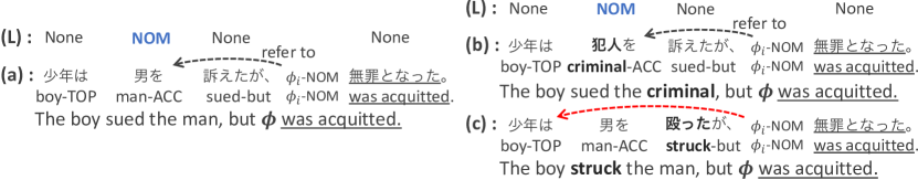
Figure 1: Examples of anaphoric relations in augmented sentences by CDA. “(L)”: the gold labels. “(a)”: the original sentence. “(b)”: successfully augmented sentence. “(c)”: undesirable augmented sentence.

2 Related Work

ZAR has been studied in the Asian languages, such as Chinese [Converse, 2005, Zhao and Ng, 2007, Kong and Zhou, 2010, Chen and Ng, 2016, Yin et al., 2018], Japanese [Seki et al., 2002, Isozaki and Hirao, 2003, Iida et al., 2003, Iida et al., 2006, Iida et al., 2007, Iida et al., 2015, Iida et al., 2016], and Korean [Han, 2006], and Romance languages, such as Italian [Rodríguez et al., 2010, Iida and Poesio, 2011] and Spanish [Ferrández and Peral, 2000, Palomar et al., 2001]. While many recent studies adopted supervised learning methods, the amount of labeled data is not sufficient to teach a model about knowledge for accurately resolving anaphoric relations. Some studies tried extracting and exploiting such knowledge from large-scale unlabeled data (e.g., case frame construction [Sasano et al., 2008, Sasano and Kurohashi, 2011, Yamashiro et al., 2018], pseudo training data generation  [Liu et al., 2017], and semi-supervised adversarial training [Kurita et al., 2018]). Although findings on using unlabeled data for ZAR have been accumulated, the automatic augmentation of labeled data has been underinvestigated. One reason for this is the difficulty in producing high-quality pseudo data from its original labeled data.

Some existing methods of text data augmentation take advantage of hand-crafted resources [Zhang et al., 2015, Wang and Yang, 2015] and rules [Fürstenau and Lapata, 2009, Kafle et al., 2017]. With the recent advances of LMs [Peters et al., 2018, Devlin et al., 2019], CDA, which is a new method using LMs, has been proposed and reported to effectively increase labeled data in several NLP tasks [Kobayashi, 2018, Wu et al., 2019, Gao et al., 2019]. This method offers a variety of good substitutes of original tokens without any hand-crafted resources. In ZAR, a key to performance improvement is training a model on anaphoric relations in various contexts. However, the original labeled data over a limited portion of contextual diversity. Here, CDA is a promising tool for producing good contextual variations of each original sentence. Considering this advantage, we introduce CDA to ZAR and provide extensive empirical results to encourage the future exploration of this direction.

3 Japanese Zero Anaphora Resolution

3.1 Problem Formulation and Notation

Japanese ZAR is often formulated as a part of the predicate-argument structure (PAS) analysis, which includes the task of detecting syntactically depending arguments (DEPs), in addition to ZAR. Given a sentence $\bm{X}$ and a list of predicates $\bm{p}$, the Japanese PAS analysis task aims to identify the head words of nominative (NOM), accusative (ACC), and dative (DAT) arguments for each predicate. Our task definition strictly follows that of previous studies [Iida et al., 2015, Ouchi et al., 2017, Matsubayashi and Inui, 2017, Matsubayashi and Inui, 2018], making our results comparable with those published previously.

In the following sections we consider that the input sentence $\bm{X}=(\bm{x}_{1},\dots,\bm{x}_{I})$ consists of a sequence of one-hot vectors $\bm{x}_{i}\in\{0,1\}^{|\mathcal{V}|}$, each of which represents a word in the sentence. $\mathcal{V}$ denotes a vocabulary set. Each sentence comprises $J$ predicates $\bm{p}=(p_{1},\dots,p_{J})$, where $p_{j}\in\mathbb{N}$ is a natural number indicating a predicate position.

3.2 Baseline Model

The baseline model employed in our experiments (hereinafter referred to as MP-masked language model (MP-MLM)) is based on the multi-predicate (MP) model proposed by Matsubayashi and Inui [Matsubayashi and Inui, 2018]. Figure 2 depicts an overview of the MP-MLM. The only difference is that our MP-MLM uses a sequence of the final hidden states of a pretrained MLM, such as BERT [Devlin et al., 2019], as the input for the MP model, whereas the original MP model uses conventional non-contextual word embeddings as the input layer. The MP-MLM is a sequential labeling model. Given a sentence $\bm{X}$, predicate positions $\bm{p}$ and a target predicate position $p_{j}\in\bm{p}$ formally. The MP-MLM models a conditional probability $P({y}_{i,j}|\bm{X},\bm{p},i,j)$. Here, ${y}_{i,j}\in\{\texttt{NOM},\texttt{ACC},\texttt{DAT},\texttt{NONE}\}$ is an argument label for a pair of $i$th word $\bm{x}_{i}$ and $j$th predicate.

The MP-MLM encodes an input $\bm{X}$ as follows:

$$\bm{E}=\operatorname*{\mathrm{MLM}}(\bm{X}),$$ (1)

where $\operatorname*{\mathrm{MLM}}$ represents a function computing its final hidden states $\bm{E}=(\bm{e}_{1},\dots,\bm{e}_{I})$. Here, $\bm{e}_{i}\in\mathbb{R}^{D}$, and $D$ is the hidden state size. Each state $\bm{e}_{i}$ is then concatenated with two binary values $b^{target}_{i}$ and $b^{others}_{i}$, where $b^{target}_{i}$ represents whether or not the word is the target predicate, and $b^{others}_{i}$ represents whether or not the word is the predicate. This concatenation operation is presented as follows:

$$\bm{h}^{0}_{i,j}=\bm{e}_{i}\oplus b^{\mathrm{target}}_{i}\oplus b^{\mathrm{others}}_{i},$$ (2)

$$b^{\mathrm{target}}_{i}= \begin{cases}1&(\mbox{if}\quad i=p_{j})\\ 0&(\mbox{otherwise}),\end{cases}$$ (3)

$$b^{\mathrm{others}}_{i}= \begin{cases}1&(\mbox{if}\quad i\in\bm{p})\\ 0&(\mbox{otherwise}),\end{cases}$$ (4)

where $\oplus$ denotes the concatenation operation, and $\bm{h}^{0}_{i,j}\in\mathbb{R}^{D+2}$ denotes the output of this concatenation operation. The obtained vectors are then fed into the $k$-layer bi-directional RNN (BiRNN) with residual connections [He et al., 2016] and alternating directions [Zhou and Xu, 2015] as follows:

$$\bm{h}^{1}_{i,j}= \textrm{RNN}^{1}(\bm{h}^{0}_{i,j},\bm{h}^{1}_{i-1,j}),$$ (5)

$$\bm{h}^{k}_{i,j}= \begin{cases}\bm{h}^{k-1}_{i,j}+\textrm{RNN}^{k}(\bm{h}^{k-1}_{i,j},\bm{h}^{k}_{i-1,j})&(k\mbox{ is odd})\\ \bm{h}^{k-1}_{i,j}+\textrm{RNN}^{k}(\bm{h}^{k-1}_{i,j},\bm{h}^{k}_{i+1,j})&(k\mbox{ is even})\end{cases}(k\geq 2),$$ (6)

where $\bm{h}^{k}_{i,j}\in\mathbb{R}^{M}$ denotes the output of the $k$th RNN layer, and $\textrm{RNN}^{k}$ denotes the function representing the $k$th RNN layer. Gated recurrent units [Cho et al., 2014] are used for RNN cells. A four-dimensional vector representing a probability distribution $P({y}_{i,j}|\bm{X},\bm{p},i,j)\in\mathbb{R}^{4}$ is then obtained as follows by applying a softmax layer to the output $\bm{h}^{K}_{i,j}\in\mathbb{R}^{M}$:

$$P({y}_{i,j}|\bm{X},\bm{p},i,j)=\mathrm{softmax}(\bm{W}\bm{h}^{K}_{i,j}),$$ (7)

where $\bm{W}\in\mathbb{R}^{4\times M}$ is a classification layer. For each argument slot $l\in\{\texttt{NOM},\texttt{ACC},\texttt{DAT}\}$ of each predicate, we eventually select a word $\bm{x}_{i}$ with the maximum probability of $P({y}_{i,j}=l|\bm{X},\bm{p},i,j)$ as an argument if the probability exceeds a threshold $\theta_{l}\in\mathbb{R}$; otherwise, the slot remains empty.

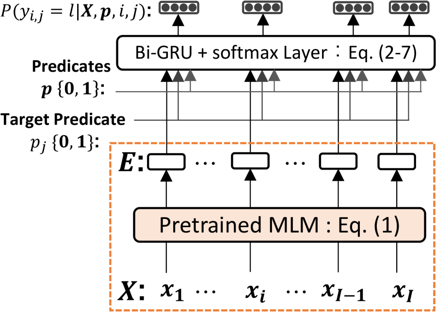
(a) Baseline

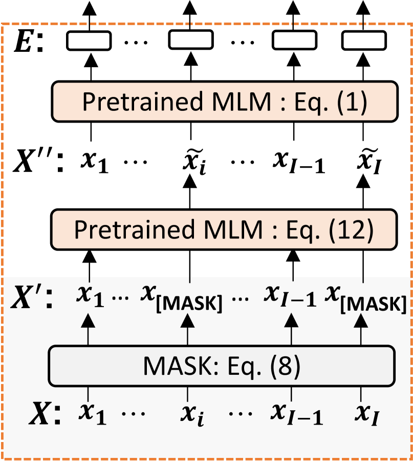
(b) CDA

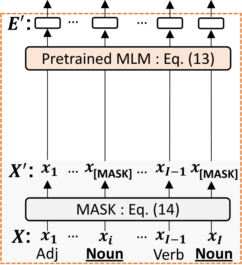
(c) Masking

Figure 2: Overview of our models. (a): the baseline model (MP-MLM) for Japanese ZAR. (b): the integration of a standard CDA method into the baseline. (c): proposed data augmentation method.

4 Method

In this section, we first review an existing standard CDA method (Section 4.1), which is our starting point of data augmentation for ZAR. We then discuss the quantitative and qualitative aspects of CDA: (i) computational inefficiency of symbolic replacement and (ii) change of antecedents. Considering these aspects, we improve a standard CDA method with two methods, namely [MASK]-based augmentation (Section 4.2) and linguistically-controlled masking (Section 4.3).

4.1 Contextual Data Augmentation (CDA)

The idea underlying CDA aims to replace token(s) in a given sentence with other token(s) that seem probable in a given context. Sentences that contain some replaced tokens are regarded as new training instances. The alternative tokens for the replacement are selected on the basis of the probability distribution output from a pretrained LM. For example, in existing studies, bi-directional RNN-based LMs [Kobayashi, 2018] and MLM [Wu et al., 2019] have been used to compute the distribution. Our CDA formulation closely follows that proposed by Wu et al. [Wu et al., 2019]. We first replace token(s) in $\bm{X}$ with [MASK] and obtain $\bm{X}^{\prime}$ as follows:

$$\bm{X}^{\prime}=(\bm{x}_{1}^{\prime},\dots,\bm{x}_{I}^{\prime})\quad\mbox{where}\quad\bm{x}^{\prime}_{i}= \begin{cases}\bm{x}_{i}&(r_{i}=0)\\ \bm{x}_{\texttt{[MASK]}{}}&(r_{i}=1),\end{cases}$$ (8)

$$r_{i}\sim \mathrm{Bernoulli(\alpha)},$$ (9)

where $\alpha$ is the probability of the replacement with [MASK]. We then feed $\bm{X}^{\prime}$ to MLM to obtain a sequence of the final hidden states $(\bm{e}^{\prime}_{1},\dots,\bm{e}^{\prime}_{I})$, where $\bm{e}^{\prime}_{i}\in\mathbb{R}^{D}$. The MLM then computes the token for replacement $\tilde{\bm{x}}_{i}$ as

$$P_{i} =\mathrm{softmax}(\bm{W}_{\textrm{MLM}}\bm{e}^{\prime}{}_{i}),$$ (10)

$$\tilde{\bm{x}}_{i} =\mathrm{F}(P_{i}),$$ (11)

where $\bm{W}_{\textrm{MLM}}\in\mathbb{R}^{\lvert V\rvert\times D}$ denotes a classification layer of the pretrained MLM; $P_{i}\in\mathbb{R}^{\lvert V\rvert}$ denotes the probability distribution over the vocabulary; and $\mathrm{F}$ denotes a function for selecting one word from $P_{i}$. [MASK]s are then replaced with the predicted tokens to obtain a new sequence $\bm{X}^{\prime\prime}$ as follows:

$$\bm{X}^{\prime\prime}=(\bm{x}_{1}^{\prime\prime},\dots,\bm{x}_{I}^{\prime\prime})\quad\mbox{where}\quad\bm{x}_{i}^{\prime\prime} =\begin{cases}\bm{x}_{i}&(\mbox{if}\quad\bm{x}_{i}^{\prime}\neq\bm{x}_{\texttt{[MASK]}{}})\\ \tilde{\bm{x}}_{i}&(\mbox{otherwise}),\end{cases}$$ (12)

Finally, $\bm{X}^{\prime\prime}$ is paired with the original gold labels of $\bm{X}$ and regarded as a new training instance.

As we mentioned in Section 1, we improved the above CDA method. First, we improved the computational efficiency. While good substitutes of the original tokens can be produced by using a gigantic MLM, the computational cost for training the model increases, and this cost cannot be ignored. Although the amount of training data of the Japanese ZAR is relatively small, the computational cost can be enormous when one wants to conduct multiple experiments with various settings. In Section 5, we indeed conduct extensive experiments to explore the use of CDA for ZAR. We design a technique that halves the computational cost of incorporating the abovementioned CDA method into the baseline model. This technique improves the performance of ZAR more effectively than a standard CDA on the same amount of augmented training data. Second, we improved the controllability. Our preliminary experiments suggested that replacing certain types of tokens is likely to change the antecedent of each zero pronoun. If another token (a token different from the original one) can be interpreted as the antecedent after the replacement, the original label will make no sense, which leads to a model being confused. We design herein a method that enables controlling the types of tokens to be replaced (Section 4.3).

4.2 [MASK]-based Augmentation

We present the [MASK]-based augmentation and simplify the integration of the original CDA into the baseline model (Section 3.2) for computational efficiency. Figure 2 shows an overview of the method. Instead of using the sequence $\bm{X}^{\prime\prime}$ with token-replacement, we used the masked sequence $\bm{X}^{\prime}$ (Equation 8) as the new training data. That is, while an MLM has to be run over each input sequence twice (for predicting substitutes and computing their feature representations) when using the original CDA, the MLM has to be run only once in our simplified one. This one-pass running of the MLM halves the computational cost of the original CDA. In particular, the masked sequence $\bm{X}^{\prime}$ is fed into the MLM, and a sequence of the final hidden states of MLM $\bm{E}^{\prime}$ is obtained:

$$\bm{E}^{\prime} =\operatorname*{\mathrm{MLM}}(\bm{X}^{\prime}).$$ (13)

The remaining computations are the same as those for the MP-MLM described in Section 3.2. Note that the MLM is pretrained to fill the [MASK] with a token that is probable in a given context. We can expect that the final hidden state of the [MASK] is an abstract and a mixture of contextually possible word representations for a given context. This is not the case for the original CDA approach (Figure 2), where the tokens are symbolically replaced with other tokens.

4.3 Linguistically-controlled Masking

We introduce and add a new function, called linguistically-controlled masking, to the abovementioned framework [MASK]-based augmentation. This function enables us to freely choose which types of tokens will be the target for replacement. As explained in Figure 1 in Section 1, replacing certain types of tokens is likely to change the antecedent of each zero pronoun. Here, instead of replacing arbitrary tokens, we utilize POS tags to control the types of tokens to be replaced. We particularly add the POS constraint to Equation 8:

$$\bm{X}^{\prime}=(\bm{x}_{1}^{\prime},\dots,\bm{x}_{I}^{\prime})\quad\mbox{where}\quad\bm{x}^{\prime}_{i}= \begin{cases}\bm{x}_{i}&(r_{i}=0)\\ \bm{x}_{\texttt{[MASK]}{}}&(r_{i}=1\quad\mbox{and}\quad s_{i}\in\mathcal{S}),\end{cases}$$ (14)

$$r_{i}\sim \mathrm{Bernoulli(\alpha)},$$ (15)

$$s_{i}= \psi(\bm{X},i),$$ (16)

where $\mathcal{S}$ denotes a set of target POS tags to be replaced, and $\psi$ denotes a function for obtaining the POS tag $s_{i}$ of the $i$th word $\bm{x}_{i}$. In other words, $\bm{x}_{i}$ is replaced with [MASK] only if its POS tag belongs to the set of target POS tags to be replaced. The remaining operations are the same as those for the MP-MLM described in Section 3.2.

5 Experiments

Split		NOM	ACC	DAT
Training	DEP	36,877	24,624	5,741
	ZAR	12,201	2,130	464
Validation	DEP	7,414	5,044	1,611
	ZAR	2,660	443	138
Test	DEP	13,982	9,395	2,488
	ZAR	4,990	903	260

Table 1: Statistics on NAIST Text Corpus 1.5

Set of POS tags	Ratio (%)	#Tokens
$\mathcal{S}_{\mathrm{noun}}$	43.54	954,816
$\mathcal{S}_{\mathrm{verb}}$	11.34	248,777
$\mathcal{S}_{\mathrm{particle}}$	25.37	556,296
$\mathcal{S}_{\mathrm{symbol}}$	11.78	258,393
$\mathcal{S}_{\mathrm{all}}$	100.00	2,192,900

Table 2: Number of tokens whose POS tag belongs to a set of POS tags: each number is counted on the training set of NTC 1.5.

Configurations	Values
RNN Cell	Bi-GRU [Matsubayashi and Inui, 2018], $k=10$
Optimizer	Adam [Kingma and Ba, 2015] ($\beta_{1}=0.9,\beta_{2}=0.98,\epsilon=1\times 10^{-8}$)
Learning Rate Schedule	Same as described in Appendix A of Matsubayashi and Inui [Matsubayashi and Inui, 2018]
Number of Epochs	150
Stopping Criterion	Same as described in Appendix A of Matsubayashi and Inui [Matsubayashi and Inui, 2018]
Gradient Clipping	1.0
BERT Fine-tuning	None: All BERT parameters are fixed

Table 3: List of hyper-parameters

In this section, we first investigate the effectiveness of [MASK]-based augmentation by comparing it with the baseline CDA (Section 4.1) on the validation set (Section 5.2). We then investigate the relationships between performance gain and each POS category to be replaced with some masking probability to find the best configuration of linguistically-controlled masking over the validation set (Section 5.3). Finally, we compare the best configured model with the other existing models over a test set (Section 5.4).

5.1 Experimental Configuration

The NAIST Text Corpus (NTC) 1.5 [Iida et al., 2010, Iida et al., 2017] with the standard dataset splits proposed by Taira et al. [Taira et al., 2008] was used for the experiments. NTC 1.5 is a benchmark dataset commonly adopted by previous studies [Ouchi et al., 2017, Matsubayashi and Inui, 2018, Omori and Komachi, 2019]. Table 2 presents the number of instances in NTC 1.5, and Table 2 presents the number of tokens whose POS tag appears in the NTC 1.5 training set.

We used both the modified sentence $\bm{X}^{\prime}$ and the original sentence $\bm{X}$ in a 1:1 ratio for training. Each model was trained using 10 different random seeds. The POS tags from the NTC gold standard tags were used in the experiments. The $\operatorname*{arg\,max}$ function was employed as $\mathrm{F}$ in Equation (11), which denotes the function for selecting the most probable word from the probability distribution. The average $\mathrm{F}_{1}$-scores were reported for both ZAR and DEP. The BERT [Devlin et al., 2019] pretrained using the Japanese Wikipedia [Shibata et al., 2019] was employed as the MLM. The BERT parameters were kept fixed throughout the experiments. The target predicate was never masked. Table 3 shows the set of employed hyper-parameters.

5.2 Effectiveness of [MASK]-based Augmentation

Method	ZAR $\mathrm{F}_{1}$	DEP $\mathrm{F}_{1}$	ALL $\mathrm{F}_{1}$
Baseline	64.08	92.82	87.43 $\pm$0.14
Baseline (2x)	63.55	92.75	87.24 $\pm$0.17
CDA	64.30	92.79	87.42 $\pm$0.18
Masking	64.89	92.94	87.64 $\pm$0.09

Table 4: $\mathrm{F}_{1}$ scores on the NTC 1.5 validation set. Bold values indicate best results in the same column.

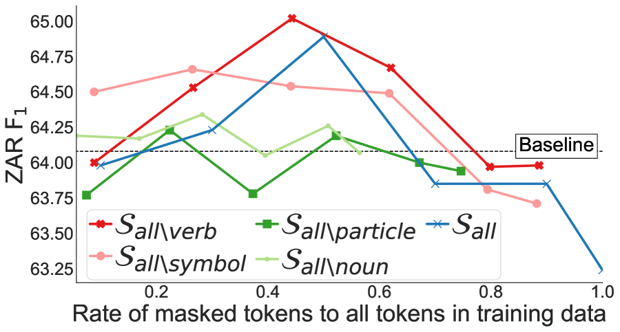
Figure 3: The effect of changing masking probability $\alpha$ on ZAR $\mathrm{F}_{1}$

We investigated the effectiveness of the [MASK]-based augmentation, where all tokens were considered as targets for replacement. The best masking probability $\alpha$ was identified from {0.1, 0.3, 0.5, 0.7, 0.9, 1.0}. The masking positions were fixed for each epoch to reduce the computational cost. Hereafter, we refer to the proposed method as Masking, which was compared to the base CDA. In the CDA, all [MASK] tokens were filled simultaneously. We also report herein on the performance of the Baseline (i.e., MP-MLM) with double amount of training data, namely, Baseline (2x). Baseline (2x) aims to conduct a fair comparison using the same amount of labeled data as those used by CDA and Masking.

Table 3 shows the results. Masking achieved the best F₁ scores for all the categories. Note that Baseline (2x) did not outperform Baseline, indicates that the improvement was achieved due to Masking rather than the increased amount of the same training instances. Masking also outperformed the base CDA, illustrating that our simplification applied to the base CDA contributed to the prediction performance and the computational efficiency.

5.3 Effectiveness of Linguistically-controlled Masking

We varied a target POS tagset for the masking and the masking probability to investigate the relationships between performance gain and each POS category. We left each one out of all the POS categories and treated the rest as targets for replacement. Let $\mathcal{S}_{all\backslash\mathrm{verb}}$ denote that all POS categories, except for the verb, are targets for replacement (i.e., “all-but-verb masking,”). We will refer to the others in the same manner. The models were trained with every possible combination of the following settings: (i) POS category {$\mathcal{S}_{all\backslash\mathrm{noun}}$, $\mathcal{S}_{all\backslash\mathrm{verb}}$, $\mathcal{S}_{all\backslash\mathrm{particle}}$, $\mathcal{S}_{all\backslash\mathrm{symbol}}$, $\mathcal{S}_{\mathrm{all}}$} and (ii) masking probability $\alpha$: {0.1, 0.3, 0.5, 0.7, 0.9, 1.0}.

Figure 3 shows the relationships between ZAR $\mathrm{F}_{1}$ and the number of masked tokens using each POS-controlled masking. The horizontal axis represents the proportion of masked tokens to all tokens in the training data. Here, all-but-verb masking $\mathcal{S}_{all\backslash\mathrm{verb}}$ tended to achieve the best results, and all-but-symbol masking $\mathcal{S}_{all\backslash\mathrm{symbol}}$ was on par or slightly better than $\mathcal{S}_{\mathrm{all}}$. While these three outperformed Baseline in most cases, the others (i.e., $\mathcal{S}_{all\backslash\mathrm{noun}}$ and $\mathcal{S}_{all\backslash\mathrm{particle}}$) did not. These performance differences were also observed under the condition of the same number of masked tokens. Controlling masked tokens by their POS category affected the performance. Moreover, a relatively high masking probability of approximately $0.5$ tends to allow the realization of a better performance.

Table 5 shows the result of the model achieving the highest ZAR $\mathrm{F}_{1}$ for each POS-controlled masking. Here, we also trained masking models with a single target POS category (e.g., $\mathcal{S}_{\mathrm{verb}}$). The results show that all-but-verb masking $\mathcal{S}_{all\backslash\mathrm{verb}}$ achieved a better ZAR $\mathrm{F}_{1}$ than Baseline. By contrast, only-verb masking $\mathcal{S}_{\mathrm{verb}}$ did not improve the performance compared with Baseline. These results imply that verbs should not be the targets for replacement. In this way, the POS category-based analysis and observation are facilitated by our linguistically-controlled masking. A more detailed analysis is provided in Section 6.

5.4 Comparison with the Existing Models

Method	ZAR $\mathrm{F}_{1}$	DEP $\mathrm{F}_{1}$	ALL $\mathrm{F}_{1}$
Baseline	64.08	92.82	87.43 $\pm$0.14
$\mathcal{S}_{\mathrm{all}}$	64.89	92.94	87.64 $\pm$0.09
$\mathcal{S}_{\mathrm{noun}}$	64.62	92.87	87.53 $\pm$0.09
$\mathcal{S}_{\mathrm{verb}}$	64.15	92.78	87.35 $\pm$0.09
$\mathcal{S}_{\mathrm{particle}}$	64.31	92.82	87.43 $\pm$0.19
$\mathcal{S}_{\mathrm{symbol}}$	64.12	92.74	87.29 $\pm$0.16
$\mathcal{S}_{all\backslash\mathrm{noun}}$	64.34	92.85	87.44 $\pm$0.16
$\mathcal{S}_{all\backslash\mathrm{verb}}$	65.02	92.96	87.67 $\pm$0.11
$\mathcal{S}_{all\backslash\mathrm{particle}}$	64.23	92.83	87.44 $\pm$0.15
$\mathcal{S}_{all\backslash\mathrm{symbol}}$	64.66	92.98	87.59 $\pm$0.19
$\mathcal{S}_{all\backslash(\mathrm{verb}\cup\mathrm{symbol})}$	64.81	92.97	87.72 $\pm$0.16

Table 5: $\mathrm{F}_{1}$ scores for each POS-controlled masking on the NTC 1.5 validation set. The method names denote a set of target POS for masking. Bold values indicate best results in the same column.

	ZAR				DEP
Method	ALL	NOM	ACC	DAT	ALL	ALL	SD
Single Model
Matsubayashi and Inui [Matsubayashi and Inui, 2018]	55.55	57.99	48.9	23	90.26	83.94	$\pm$0.12
Omori and Komachi [Omori and Komachi, 2019]	53.50	56.37	45.36	8.70	90.15	83.82	$\pm$0.10
Baseline†	63.89	66.45	57.2	27	92.24	86.85	$\pm$0.11
CDA†	63.87	66.16	58.5	29	92.27	86.84	$\pm$0.19
Masking ($\mathcal{S}_{all\backslash\mathrm{verb}}$)†	64.15	66.60	57.9	29	92.46	86.98	$\pm$0.13
Ensemble Model
Matsubayashi and Inui [Matsubayashi and Inui, 2018]∗	58.07	60.21	52.5	26	91.26	85.34	-
Baseline†∗	66.45	68.91	60.1	30	93.07	88.06	-
Masking ($\mathcal{S}_{all\backslash\mathrm{verb}}$)†∗	67.35	69.85	61.2	28	93.32	88.43	-

Table 6: $\mathrm{F}_{1}$ scores on the NTC 1.5 test set. Bold value indicate the best results in the same column group. $\dagger$: result from our experiment. $*$: ensemble models. The improvement of Masking over the Baseline is statistically significant in both overall F1 score and ZAR F1 score ($p<0.05$) with a permutation test.

We compared the model built by all-but-verb masking $\mathcal{S}_{all\backslash\mathrm{verb}}$, which achieved the best ZAR $\mathrm{F}_{1}$ on the validation set (Table 5), with state-of-the-art models [Matsubayashi and Inui, 2018, Omori and Komachi, 2019] on the test set. Table 6 shows the results. We refer to our method of combining [MASK]-based augmentation and linguistically-controlled masking in the optimal setting as Masking ($\mathcal{S}_{all\backslash\mathrm{verb}}$). Our Baseline already outperformed the state-of-the-art results by a large margin. When new techniques are only evaluated on very basic models, determining how much (if any) improvement will carry over to stronger models can be difficult [Denkowski and Neubig, 2017, Suzuki et al., 2018]. In contrast to this concern, Masking ($\mathcal{S}_{all\backslash\mathrm{verb}}$) consistently achieved the statistically significant improvements over the strong Baseline in both single and ensemble-model settings. This solid finding is likely to be generalizable to other strong models. On the contrary, the ZAR $\mathrm{F}_{1}$ of the CDA was on par with that of Baseline, which shows that the symbolic replacement of tokens is not effective.

6 Analysis of Augmented Data

In this section, we analyze the actual instances augmented by linguistically-controlled masking. The model built by all-but-verb masking $\mathcal{S}_{all\backslash\mathrm{verb}}$ achieved the best ZAR $\mathrm{F}_{1}$; hence, we further investigated the negative effect of verb replacement. We did this by observing the actual instances produced by $\mathcal{S}_{all\backslash\mathrm{verb}}$ and verb-only masking $\mathcal{S}_{\mathrm{verb}}$. Figure 4 depicts the three types of sentences of these two models, that is, the original ones $\bm{X}$, the masked ones $\bm{X}^{\prime}$, and those with some symbolically replaced tokens $\bm{X}^{\prime\prime}$. Note that although our method did not use any symbolic substitutions $\bm{X}^{\prime\prime}$ for predicting the of zero anaphora (Section 4.2), they were produced only for the analysis. Looking at the symbolic token generated from each mask provides us an intuition on the feature vector of each mask. For example, if the token exist is generated from a mask, we can interpret that its corresponding vector approximately represents the meaning of exist.

In the original sentence $\bm{X}$, the nominative argument of the target predicate noticeable was realized as a zero pronoun $\phi$, and its antecedent was The scratches. In the sentence generated by $\mathcal{S}_{\mathrm{verb}}$, the symbolic token exist filled the [MASK] ($\bm{X}_{1}^{\prime\prime}$), and the semantic structure of the sentence, especially the original relation between the two predicates (verbs) be fixed and noticeable, was changed. The antecedent can be interpreted as null, which was changed from the original one The scratches. In contrast, in the sentence generated by $\mathcal{S}_{all\backslash\mathrm{verb}}$ ($\bm{X}_{2}^{\prime\prime}$), the antecedent of the zero pronoun was not changed, even though half of the tokens in the sentence has been replaced. The antecedent was that, which aligned with the original token (position), scratches. The original relation between the two predicates, be fixed and noticeable, still remained. In addition, the pretrained MLM generated the tokens surrounding these predicates, such that the context drastically changed from the original one the scratches can’t be repaired, but … to if that gets fixed, …. Such a contextual variation plays an important role for improving the robustness and the coverage of a ZAR model, even if the meaning is slightly unnatural. This can be a reason for the results in Section 4.3, indicating that the setting of a high masking probability (approximately $0.5$) and all-but-verb masking $\mathcal{S}_{all\backslash\mathrm{verb}}$ achieves a better performance.

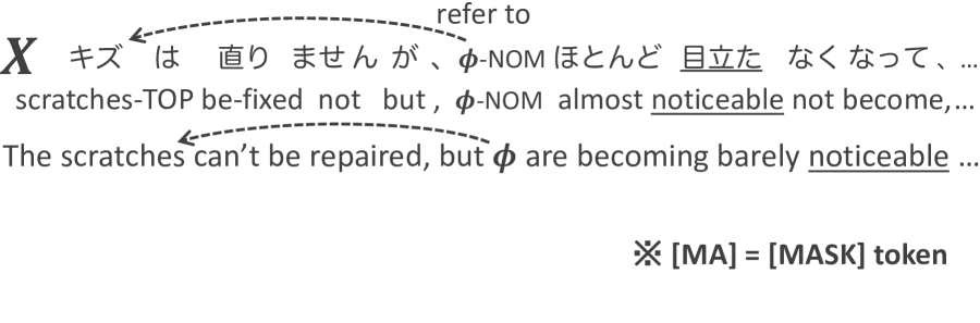
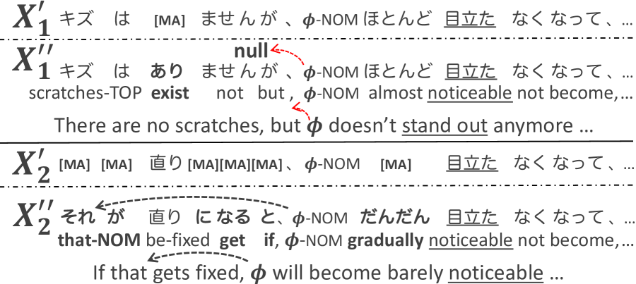
Figure 4: Examples of pseudo data created by data augmentation. $\bm{X}^{\prime}$ indicates the pseudo data in Masking. $\bm{X}^{\prime\prime}$ indicates the pseudo data in CDA. $\bm{X}_{1}^{\prime}$ and $\bm{X}_{1}^{\prime\prime}$ are output of $\mathcal{S}_{\mathrm{verb}}$. $\bm{X}_{2}^{\prime}$ and $\bm{X}_{2}^{\prime\prime}$ are output of $\mathcal{S}_{all\backslash\mathrm{verb}}$.

7 Discussion

We tackled a data scarcity problem on the Japanese ZAR through data augmentation. We specifically improved the CDA for the ZAR from the quantitative and qualitative aspects: [MASK]-based augmentation (Section 4.2) and linguistically-controlled masking (Section 4.3).

Summary of Empirical Results    We obtained the following results from the extensive experiments (Section 5):

• Effectiveness of [MASK]-based augmentation: efficiently enables integrating a gigantic MLM and achieves statistically significant improvements over a strong baseline and standard CDA (Table 3);

• Effects of masking probability: a relatively high masking probability leads to a performance gain (Figure 3);

• Advantage of linguistically-controlled masking: this enables controlling which types of tokens to be replaced. Verbs should not be targets for replacement (Table 5).

Suggestions from In-depth Analysis    The analysis on the actual augmented data (Section 6) provided the future ZAR research with two suggestions:

• Keep the original semantic structure, especially the relation between the predicates (verbs); otherwise, the original antecedent of a zero pronoun is likely to be changed.

• Generate contextual variations relatively far from an original sentence by adjusting the masking probability while keeping its original semantic structure.

Future Work    We found herein the interesting phenomenon of change of antecedents and analyzed it by observing several actual instances. One interesting direction of the future research is the quantitative investigation of this phenomenon and the revelation of the relationships between the change of antecedents and the types of tokens to be replaced. We controlled the token replacement positions by POS tags. The other possible method of determining these positions is to use a syntactic structure, such as dependency relations, and relative distances from the target predicate. We plan to explore such linguistic features to control the replacement.

Appendix A Word Replacement Approaches

This section compares alternative approaches of the CDA method described in Section 4.1. We compare several different procedures for filling [MASK] tokens using the pretrained MLM. Specifically, we consider two aspects: (i) how many [MASK] tokens to fill simultaneously and (ii) how to determine a word symbol in each time step.

For (i) how many [MASK] tokens to fill simultaneously, we compare the following two methods:

• Single: The overview of this method is presented in Figure 5. Suppose that a masked sentence $\bm{X}^{\prime}$ contains $N$ [MASK] tokens, we first create $(\bm{X}_{1}^{\prime},\dots,\bm{X}_{N}^{\prime})$ from $\bm{X}^{\prime}$. Here, each $\bm{X}_{n}^{\prime}$ contains a single [MASK] token and the rest of tokens are from the original sentence $\bm{X}$. Note that the position of the [MASK] token is unique for each $\bm{X}_{n}^{\prime}$. We then feed $(\bm{X}_{1}^{\prime},\dots,\bm{X}_{N}^{\prime})$ to MLM independently and fill each [MASK] token with another token to obtain $(\bm{X}_{1}^{\prime\prime},\dots,\bm{X}_{N}^{\prime\prime})$. Finally, we merge the outputs $(\bm{X}_{1}^{\prime\prime},\dots,\bm{X}_{N}^{\prime\prime})$ to construct a symbolically modified sentence $\bm{X}^{\prime\prime}$.

• Multi: The overview of this method is presented in Figure 5. Given a masked sentence $\bm{X}^{\prime}$, we feed $\bm{X}^{\prime}$ to MLM and fill all [MASK] tokens simultaneously. The output of MLM is a symbolically modified sentence $\bm{X}^{\prime\prime}$.

For (ii) how to determine a word symbol in each time step, we compare the following two methods:

• Sample: Following Wang and Cho [Wang and Cho, 2019], we determine the output symbol by sampling a word from the probability distribution over vocabulary that is computed by pretrained MLM.

• Argmax: From the probability distribution over the vocabulary, we determine the output symbol by choosing the token with the highest probability.

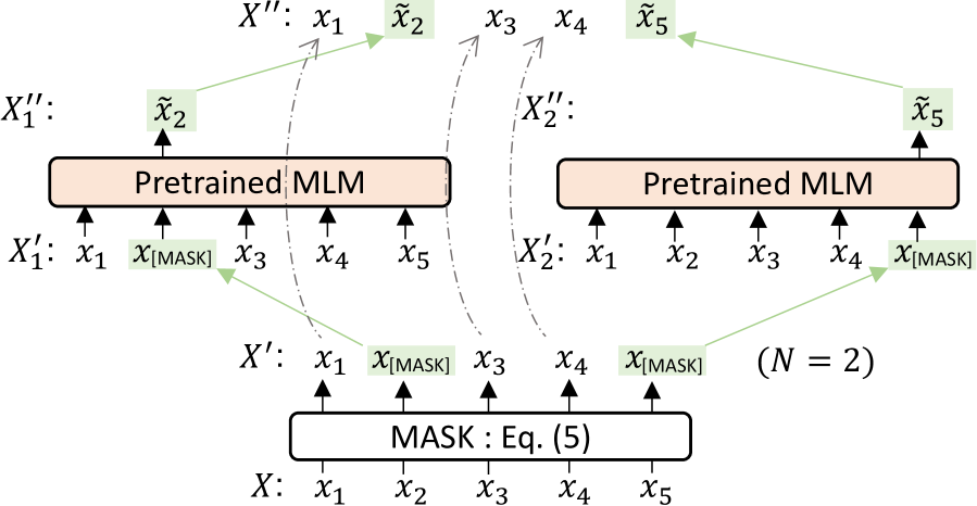
(a) SINGLE

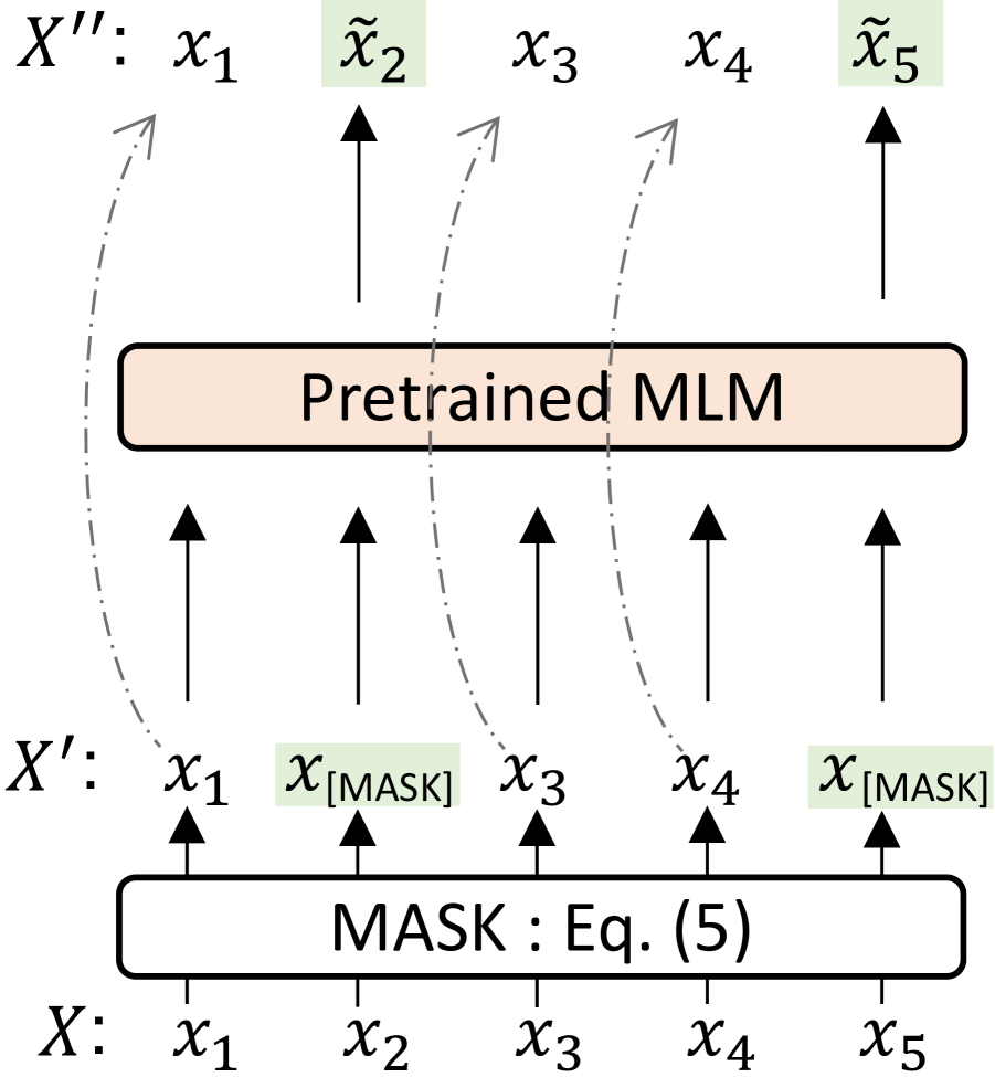
(b) MULTI

Figure 5: Overview of two replacement approaches.

Method	ZAR $\mathrm{F}_{1}$	DEP $\mathrm{F}_{1}$	ALL $\mathrm{F}_{1}$	SD
Single+Argmax	63.59	92.62	87.16	$\pm$0.12
Single+Sample	63.58	92.55	87.14	$\pm$0.16
Multi+Argmax	64.47	92.70	87.37	$\pm$0.15
Multi+Sample	63.18	92.25	86.84	$\pm$0.21

Table 7: $\mathrm{F}_{1}$ scores on the NTC 1.5 validation set. Bold values indicate the best results in the same column group.

Table 7 shows the result of the combinations of these two aspects. In this experiment, the conditions of the POS category are identical across all models with the setting of $\mathcal{S}_{all\backslash(\mathrm{verb}\cup\mathrm{symbol})}$, which achieves the best overall $\mathrm{F}_{1}$ in Table 5. The Table 7 presents that the combination of Multi and Argmax, namely, Multi+Argmax achieves the best performance. Thus, we used the Multi+Argmax setting for CDA in the experiment of Section 5.4.

References

- [Chen and Ng, 2014] Chen Chen and Vincent Ng. 2014. Chinese Zero Pronoun Resolution: An Unsupervised Approach Combining Ranking and Integer Linear Programming. In Twenty-Eighth AAAI Conference on Artificial Intelligence.
- [Chen and Ng, 2015] Chen Chen and Vincent Ng. 2015. Chinese Zero Pronoun Resolution: A Joint Unsupervised Discourse-Aware Model Rivaling State-of-the-Art Resolvers. In ACL-IJCNLP, pages 320–326.
- [Chen and Ng, 2016] Chen Chen and Vincent Ng. 2016. Chinese Zero Pronoun Resolution with Deep Neural Networks. In ACL, pages 778–788.
- [Cho et al., 2014] Kyunghyun Cho, Bart van Merrienboer, Caglar Gulcehre, Dzmitry Bahdanau, Fethi Bougares, Holger Schwenk, and Yoshua Bengio. 2014. Learning Phrase Representations using RNN Encoder-Decoder for Statistical Machine Translation. In EMNLP, pages 1724–1734.
- [Converse, 2005] Susan P. Converse. 2005. Resolving Pronominal References in Chinese with the Hobbs Algorithm. In IJCNLP-SIGHAN.
- [Denkowski and Neubig, 2017] Michael Denkowski and Graham Neubig. 2017. Stronger Baselines for Trustable Results in Neural Machine Translation. In Proceedings of the First Workshop on Neural Machine Translation, pages 18–27.
- [Devlin et al., 2019] Jacob Devlin, Ming-Wei Chang, Kenton Lee, and Kristina Toutanova. 2019. BERT: Pre-training of Deep Bidirectional Transformers for Language Understanding. In NAACL, pages 4171–4186.
- [Ferrández and Peral, 2000] Antonio Ferrández and Jesús Peral. 2000. A Computational Approach to Zero-pronouns in Spanish. In ACL, pages 166–172.
- [Fürstenau and Lapata, 2009] Hagen Fürstenau and Mirella Lapata. 2009. Semi-Supervised Semantic Role Labeling. In EACL, pages 220–228.
- [Gao et al., 2019] Fei Gao, Jinhua Zhu, Lijun Wu, Yingce Xia, Tao Qin, Xueqi Cheng, Wengang Zhou, and Tie-Yan Liu. 2019. Soft Contextual Data Augmentation for Neural Machine Translation. In ACL, pages 5539–5544.
- [Han, 2006] Na-Rae Han. 2006. Korean zero pronouns: Analysis and resolution.
- [He et al., 2016] Kaiming He, Xiangyu Zhang, Shaoqing Ren, and Jian Sun. 2016. Deep Residual Learning for Image Recognition. In CVPR, pages 770–778.
- [Iida and Poesio, 2011] Ryu Iida and Massimo Poesio. 2011. A Cross-Lingual ILP Solution to Zero Anaphora Resolution. In Proceedings of the 49th Annual Meeting of the Association for Computational Linguistics: Human Language Technologies, pages 804–813.
- [Iida et al., 2003] Ryu Iida, Kentaro Inui, Hiroya Takamura, and Yuji Matsumoto. 2003. Incorporating Contextual Cues in Trainable Models for Coreference Resolution. In Proceedings of the 2003 EACL Workshop on The Computational Treatment of Anaphora.
- [Iida et al., 2006] Ryu Iida, Kentaro Inui, and Yuji Matsumoto. 2006. Exploiting Syntactic Patterns as Clues in Zero-Anaphora Resolution. In ACL-COLING, pages 625–632.
- [Iida et al., 2007] Ryu Iida, Kentaro Inui, and Yuji Matsumoto. 2007. Zero-anaphora Resolution by Learning Rich Syntactic Pattern Features. ACM Transactions on Asian Language Information Processing, 6(4):1:1–1:22.
- [Iida et al., 2010] Ryu Iida, Mamoru Komachi, Naoya Inoue, Kentaro Inui, and Yuji Matsumoto. 2010. Annotating Predicate-Argument Relations and Anaphoric Relations: Findings from the Building of the NAIST Text Corpus. Natural Language Processing, 17(2):25–50.
- [Iida et al., 2015] Ryu Iida, Kentaro Torisawa, Chikara Hashimoto, Jong-Hoon Oh, and Julien Kloetzer. 2015. Intra-sentential Zero Anaphora Resolution using Subject Sharing Recognition. In EMNLP, pages 2179–2189.
- [Iida et al., 2016] Ryu Iida, Kentaro Torisawa, Jong-Hoon Oh, Canasai Kruengkrai, and Julien Kloetzer. 2016. Intra-Sentential Subject Zero Anaphora Resolution using Multi-Column Convolutional Neural Network. In EMNLP, pages 1244–1254.
- [Iida et al., 2017] Ryu Iida, Mamoru Komachi, Naoya Inoue, Kentaro Inui, and Yuji Matsumoto. 2017. NAIST Text Corpus: Annotating Predicate-Argument and Coreference Relations in Japanese. In Handbook of Linguistic Annotation, pages 1177–1196. Springer.
- [Isozaki and Hirao, 2003] Hideki Isozaki and Tsutomu Hirao. 2003. Japanese Zero Pronoun Resolution based on Ranking Rules and Machine Learning. In EMNLP-WS, pages 184–191.
- [Kafle et al., 2017] Kushal Kafle, Mohammed Yousefhussien, and Christopher Kanan. 2017. Data Augmentation for Visual Question Answering. In INLG, pages 198–202.
- [Kingma and Ba, 2015] Diederik Kingma and Jimmy Ba. 2015. Adam: A Method for Stochastic Optimization. In ICLR.
- [Kobayashi, 2018] Sosuke Kobayashi. 2018. Contextual Augmentation: Data Augmentation by Words with Paradigmatic Relations. In NAACL, pages 452–457.
- [Kondratyuk and Straka, 2019] Dan Kondratyuk and Milan Straka. 2019. 75 Languages, 1 Model: Parsing Universal Dependencies Universally. In EMNLP-IJCNLP, pages 2779–2795.
- [Kong and Zhou, 2010] Fang Kong and Guodong Zhou. 2010. A Tree Kernel-Based Unified Framework for Chinese Zero Anaphora Resolution. In EMNLP, pages 882–891.
- [Kurita et al., 2018] Shuhei Kurita, Daisuke Kawahara, and Sadao Kurohashi. 2018. Neural Adversarial Training for Semi-supervised Japanese Predicate-argument Structure Analysis. In ACL, pages 474–484.
- [Liu et al., 2017] Ting Liu, Yiming Cui, Qingyu Yin, Wei-Nan Zhang, Shijin Wang, and Guoping Hu. 2017. Generating and Exploiting Large-scale Pseudo Training Data for Zero Pronoun Resolution. In ACL, pages 102–111.
- [Matsubayashi and Inui, 2017] Yuichiroh Matsubayashi and Kentaro Inui. 2017. Revisiting the Design Issues of Local Models for Japanese Predicate-Argument Structure Analysis. In IJCNLP, pages 128–133.
- [Matsubayashi and Inui, 2018] Yuichiroh Matsubayashi and Kentaro Inui. 2018. Distance-Free Modeling of Multi-Predicate Interactions in End-to-End Japanese Predicate-Argument Structure Analysis. In COLING, pages 94–106.
- [Omori and Komachi, 2019] Hikaru Omori and Mamoru Komachi. 2019. Multi-Task Learning for Japanese Predicate Argument Structure Analysis. In NAACL, pages 3404–3414.
- [Ouchi et al., 2017] Hiroki Ouchi, Hiroyuki Shindo, and Yuji Matsumoto. 2017. Neural Modeling of Multi-Predicate Interactions for Japanese Predicate Argument Structure Analysis. In ACL, pages 1591–1600.
- [Palomar et al., 2001] Manuel Palomar, Antonio Ferrández, Lidia Moreno, Patricio Martínez-Barco, Jesús Peral, Maximiliano Saiz-Noeda, and Rafael Muñoz. 2001. An Algorithm for Anaphora Resolution in Spanish Texts. Computational Linguistics, 27(4):545–567.
- [Peters et al., 2018] Matthew Peters, Mark Neumann, Mohit Iyyer, Matt Gardner, Christopher Clark, Kenton Lee, and Luke Zettlemoyer. 2018. Deep Contextualized Word Representations. In NAACL, pages 2227–2237.
- [Rodríguez et al., 2010] Kepa Joseba Rodríguez, Francesca Delogu, Yannick Versley, Egon W. Stemle, and Massimo Poesio. 2010. Anaphoric Annotation of Wikipedia and Blogs in the Live Memories Corpus. In LREC.
- [Sasano and Kurohashi, 2011] Ryohei Sasano and Sadao Kurohashi. 2011. A Discriminative Approach to Japanese Zero Anaphora Resolution with Large-scale Lexicalized Case Frames. In IJCNLP, pages 758–766.
- [Sasano et al., 2008] Ryohei Sasano, Daisuke Kawahara, and Sadao Kurohashi. 2008. A Fully-Lexicalized Probabilistic Model for Japanese Zero Anaphora Resolution. In COLING, pages 769–776.
- [Seki et al., 2002] Kazuhiro Seki, Atsushi Fujii, and Tetsuya Ishikawa. 2002. A Probabilistic Method for Analyzing Japanese Anaphora Integrating Zero Pronoun Detection and Resolution. In COLING.
- [Shibata et al., 2019] Tomohide Shibata, Daisuke Kawahara, and Sadao Kurohashi. 2019. Improving Japanese Syntax Parsing with BERT. Natural Language Processing, pages 205–208.
- [Suzuki et al., 2018] Jun Suzuki, Sho Takase, Hidetaka Kamigaito, Makoto Morishita, and Masaaki Nagata. 2018. An Empirical Study of Building a Strong Baseline for Constituency Parsing. In ACL, pages 612–618.
- [Taira et al., 2008] Hirotoshi Taira, Sanae Fujita, and Masaaki Nagata. 2008. A Japanese Predicate Argument Structure Analysis using Decision Lists. In EMNLP, pages 523–532.
- [Wang and Cho, 2019] Alex Wang and Kyunghyun Cho. 2019. BERT has a Mouth, and It Must Speak: BERT as a Markov Random Field Language Model. In Proceedings of the Workshop on Methods for Optimizing and Evaluating Neural Language Generation, pages 30–36.
- [Wang and Yang, 2015] William Yang Wang and Diyi Yang. 2015. That’s So Annoying!!!: A Lexical and Frame-Semantic Embedding Based Data Augmentation Approach to Automatic Categorization of Annoying Behaviors using #petpeeve Tweets. In EMNLP, pages 2557–2563.
- [Wu et al., 2019] Xing Wu, Shangwen Lv, Liangjun Zang, Jizhong Han, and Songlin Hu. 2019. Conditional BERT Contextual Augmentation. In ICCS, pages 84–95.
- [Yamashiro et al., 2018] Souta Yamashiro, Hitoshi Nishikawa, and Takenobu Tokunaga. 2018. Neural Japanese Zero Anaphora Resolution using Smoothed Large-scale Case Frames with Word Embedding. In PACLIC.
- [Yin et al., 2018] Qingyu Yin, Yu Zhang, Weinan Zhang, Ting Liu, and William Yang Wang. 2018. Zero Pronoun Resolution with Attention-based Neural Network. In COLING, pages 13–23.
- [Zhang et al., 2015] Xiang Zhang, Junbo Zhao, and Yann LeCun. 2015. Character-level Convolutional Networks for Text Classification. In NIPS, pages 649–657.
- [Zhao and Ng, 2007] Shanheng Zhao and Hwee Tou Ng. 2007. Identification and Resolution of Chinese Zero Pronouns: A Machine Learning Approach. In EMNLP-CoNLL, pages 541–550.
- [Zhou and Xu, 2015] Jie Zhou and Wei Xu. 2015. End-to-end Learning of Semantic Role Labeling Using Recurrent Neural Networks. In ACL, pages 1127–1137.