Three discontinuous Galerkin methods for one- and two-dimensional nonlinear Dirac equations with a scalar self-interaction
Abstract
This paper develops three high-order accurate discontinuous Galerkin (DG) methods for the one-dimensional (1D) and two-dimensional (2D) nonlinear Dirac (NLD) equations with a general scalar self-interaction. They are the Runge-Kutta DG (RKDG) method and the DG methods with the one-stage fourth-order Lax-Wendroff type time discretizaiton (LWDG) and the two-stage fourth-order accurate time discretization (TSDG). The RKDG method uses the spatial DG approximation to discretize the NLD equations and then utilize the explicit multistage high-order Runge-Kutta time discretization for the first-order time derivatives, while the LWDG and TSDG methods, on the contrary, first give the one-stage fourth-order Lax-Wendroff type and the two-stage fourth-order time discretizations of the NLD equations, respectively, and then discretize the first- and higher-order spatial derivatives by using the spatial DG approximation. The stability of the 2D semi-discrete DG approximation is proved in the RKDG methods for a general triangulation, and the computational complexities of three 1D DG methods are estimated. Numerical experiments are conducted to validate the accuracy and the conservative properties of the proposed methods. The interactions of the solitary waves, the standing and travelling waves are investigated numerically and the 2D breathing pattern is observed.
keywords:
Nonlinear Dirac equation , discontinuous Galerkin method , Lax-Wendroff type time discretization , two-stage fourth-order accurate time discretization , Runge-Kutta method , solitary wave interactionMSC:
[2010] 65M60 , 35L05 , 81Q05 , 81-081 Introduction
The Dirac equation is a relativistic wave equation in particle physics, and provides a natural description of an electron [15]. It predicted the existence of “negative” states for the electron and proton, and thus successfully predicted the existence of antimatter. After Dirac found the linear equation of the electron, the basic idea of nonlinear description of the elementary particle with spin-1/2 appeared, which made it possible to consider its self-interaction [27, 20, 19], and the nonlinear Dirac (NLD) equation was proposed as a possible basis model for a unified field theory [25]. The NLD equation allows solitary wave solutions or particle-like solutions (the stable localized solutions with finite energy and charge) [36], that is to say, the particles appear as intense localized regions of field [46]. Around the 1970s and 1980s, wide interest of physicists and mathematicians was attracted by different NLD models with different self-interactions, mainly including the Thirring model [44], the Soler model [43], the Gross-Neveu model [22] (equivalent to the massless Soler model), and the bag model [33] (i.e. the solitary waves with finite compact support), especially to look for the solitary wave solutions and to investigate the related physical and mathematical properties [36]. Since entering the 21st century, the Dirac equation is used to study the structures and dynamical properties of the two-dimensional (2D) materials such as graphene and graphite [34, 8, 1, 17] and the relativistic effects in molecules in super intense lasers [18] etc. Moreover, the Bose-Einstein condensates in a honeycomb optical lattice can also be described by a NLD equation in the long wavelength, mean field limit [24]. Mathematical interests related to the NLD equation are mainly manifested in deriving the analytical solitary wave solutions, the stability analysis of the NLD solitary waves, the analysis of global well-posedness and numerical methods etc. For the 1D NLD equation (i.e. one space dimension), several analytical solitary wave solutions are derived in literature. For example, the solitary wave solutions of the 1D NLD equation with arbitrary nonlinearity was studied in [11]. However, for the high-dimensional NLD equation, there are no explicit solitary wave solutions [12]. The stability of the solitary waves can be found in [38, 13, 28]. The readers are referred to the review in [48] and references therein.
Numerical method has become one of the important tools to derive the NLD solitary wave solutions, and to investigate their stability and interaction etc. The Crank-Nicolson (CN) scheme was first proposed for the 1D Soler model and used to simulate the interaction dynamics of the NLD solitary waves in [3, 4]. Such interaction dynamics problem was carefully revisited in [39] by utilizing a fourth-order accurate RKDG method [40]. Besides the recovery of the phenomena in [3], several new ones were observed, e.g. collapse in binary and ternary collisions of two-hump NLD solitary waves [39], a long-lived oscillating state formed with an approximate constant frequency in collisions of two standing waves [40], and the full repulsion in binary and ternary collisions of out-of-phase waves [41]. Those numerical results also inferred that the two-hump profile could undermine the stability during the scattering of the NLD solitary waves. It is worth noting that the two-hump profile was first pointed out in [39] and later gotten noticed by other researchers. The multi-hump solitary waves were further studied in [49] in theory. There also exist many other numerical schemes for solving the 1D NLD equation: the split-step spectral method [21], the linearized CN scheme [2], the Legendre rational spectral method [47], the multisymplectic Runge-Kutta method [26], the adaptive mesh method [45], the time-splitting methods [32], and the compact methods [30] etc. A review of the current state-of-the-art of numerical methods for the 1D NLD equation was presented in [48]. For the 1D NLD equation with the scalar and vector self-interaction, the CN schemes, the linearized CN schemes, the odd-even hopscotch scheme, the leapfrog scheme, a semi-implicit finite difference scheme, and the exponential operator splitting schemes were extendedly proposed and analyzed in the way of the accuracy and the time reversibility as well as the conservation of the discrete charge, energy and linear momentum. For the NLD equation in the nonrelativistic limit regime, the error estimates of the CN scheme, the exponential wave integrator Fourier pseudospectral method and the time-splitting Fourier pseudospectral method were studied in [6], and a uniformly accurate multiscale time integrator pseudospectral method was proposed in [7].
Unfortunately, the existing work on numerical study of the 2D NLD equation is very limited. The integrating-factor method was studied in [14], whose authors pointed out that “it is not clear how these schemes (the RKDG methods [40]) could be generalized to higher spatial dimensions”. The standing wave solutions and vortex solutions were discussed by using the Fourier spectral method [13, 12]. Two kinds of high-order conservative schemes were obtained with the time-midpoint and the time-splitting methods as well as the operator-compensation method [31]. The aim of this paper is to extend the 1D RKDG method [40] to the 2D NLD equation with a general scalar self-interaction, and to develop the LWDG and TSDG methods, i.e. the discontinuous Galerkin (DG) schemes with the one-stage fourth-order accurate Lax-Wendroff type time discretization [35] and the two-stage fourth-order accurate time discretization [29, 51]. The RKDG method uses the spatial DG approximation to discretize the NLD equations and then utilize the explicit multistage high-order Runge-Kutta time discretization for the first-order time derivatives, while the LWDG and TSDG methods, on the contrary, first give the one-stage fourth-order Lax-Wendroff type and the two-stage fourth-order time discretizations of the NLD equations, and then discretize the first- and higher-order spatial derivatives by using the spatial DG approximation. The computational complexities of three 1D fully discrete DG methods will be theoretically estimated and their accuracy and performance will be validated by numerical experiments.
This paper is organized as follows. Section 2 introduces the NLD equations and their conservation laws, and discusses the standing and travelling wave solutions of the 2D NLD equations. Section 3 proposes three high-order accurate DG methods. The stability of the 2D semi-discrete DG method is discussed in the RKDG scheme for a general triangulation, and the computational complexities of the 1D fully discrete DG methods are also studied. Section 4 conducts some experiments to validate the accuracy and the conservative properties of our DG methods and to investigate some new phenomena. Section 5 draws the conclusion.
2 Nonlinear Dirac equations
This section introduces the 1D and 2D NLD equations with a general scalar self-interaction and the 2D standing and travelling wave solutions.
This paper is concerned with numerical methods for the 1D NLD equation
| (2.1) |
with the spinor unknown , and the 2D NLD equation
| (2.2) |
with . Here , , with , the particle mass and the nonnegative parameter , the superscripts and denote the complex conjugate transpose and the vector transpose, respectively, and
are three Pauli matrices. The term represents the general scalar self-interaction. When , Eq. (2.2) reduces to the Soler model [43].
For the 1D and 2D NLD equations (2.1) and (2.2), assuming that the solutions are smooth enough, we may derive the following proposition.
Proposition 2.1.
If holds uniformly for , then the charge and the energy are conservative, i.e. , where
Here the charge density , and and the energy density are given by
| 1D () | |||
| 2D () |
Proof.
In the following, only the case of is considered.
(i) From (2.2), one has
and its complex conjugate form
Summing up them gives
Integrating it with respect to yields the charge conservation law under the hypothesis.
Remark 2.1.
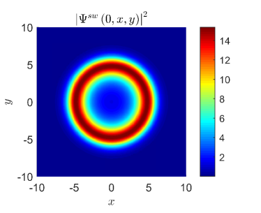
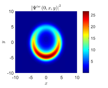
The standing and travelling wave solutions of the 1D NLD equation can be found in [11, 40, 48, 49], so that they are not presented here to avoid repetition. For the 2D NLD equation, the standing wave solution was approximately obtained in [12] by using the spectral method, the fixed point method, and the following ansatz in the polar coordinates
| (2.4) |
where and are two real-valued functions, and is the vorticity for the first spinor component. In fact, first substituting (2.4) into (2.2) gives the following system of ordinary differential equations
| (2.5) |
where , . Then using the Chebyshev spectral method to approximate the ODE system (2.5) gives the nonlinear algebraic system and the final approximate solutions are obtained by the iterative method, e.g. the fixed point method. The readers are referred to Section 3.2.2 of [12] for the details. Once we have the standing wave solution , the travelling wave solution can be obtained by using the Lorentz transformation. For example, under the Lorentz transformation with the speed of light and the relative velocity in the -direction
the travelling wave solution is gotten by
where is the Lorentz factor. Figure 2.1 shows the standing wave solution and the travelling wave solution with at , where is taken as and . The right plot shows clearly that the charge density loses symmetry in the -direction. The lack of symmetry of in the -direction is caused by the above Lorentz transformation and the difference between and in (2.4).
3 Numerical methods
This section focuses on developing three high-order accurate DG methods of the 2D NLD equation (2.2) with three time discretizations on the Cartesian grid. The 1D RKDG methods have been presented in [40], while the 1D LWDG and TSDG methods can be obtained by removing all the dependence of the wave function on from corresponding 2D schemes.
If defining , where and denote the real and imaginary parts of , respectively, , then the NLD equation (2.2) can be rewritten as follows
| (3.1) |
or in the following compact form
| (3.2) |
where , , , and
3.1 RKDG method
Let be a rectangular partition of the 2D domain and for each element , represent the space of the real-valued polynomials on of degree at most . The RKDG method [9, 10, 40] is to seek first each component of the approximate solution for any in the function space
such that for each component of any in , one has
| (3.3) |
where , is the th row vector of , , “” represents the Hadamard product, denotes the boundary of , and is the two-point numerical flux approximating the flux with the outward unit normal to the edge of the element . The numerical flux satisfies
| (3.4) |
and may be chosen as the following Lax-Friedrichs type flux [40]
| (3.5) |
Here are the limiting values of obtained from the interior () and the exterior () of , i.e.
where is the neighboring element of by a common edge , as shown in Figure 3.1, is the discrete boundary value of .

Similar to the 1D case [40], we can establish the following entropy inequality or stability of the 2D semi-discrete DG method (3.3), which implies that the discrete total charge dose not increase with respect to .
Proposition 3.1.
Proof.
For , because is arbitrary, we may choose in (3.3) as , and then have
Summing up the above four equations gets
| (3.6) |
For the edge , see Figure 3.1, by noticing (3.5), (3.4), and , we have
here and are the limiting values of from the interiors () of and , respectively, in order to distinguish the values of from the different elements. Since , we have
Combining them, summing up (3.6) on all , and noticing the boundary condition yields
This completes the proof. ∎
For the Cartesian grid, following [9], we choose the following local basis functions
where and are the spatial step sizes in and directions, respectively. Then the DG approximate solutions can be expressed as
| (3.7) |
where are the degrees of freedom to be determined. Substituting them into (3.3) gives the semi-discrete DG scheme for the degrees of freedom
| (3.8) |
where and . The integrals in (3.8) will be calculated by the -point Gauss-Legendre quadrature in each coordinate direction.
3.2 LWDG and TSDG methods
This section proposes two other DG methods, i.e. the LWDG and TSDG methods. Different from the above RKDG method, they are derived by first giving the one-stage fourth-order Lax-Wendroff type and the two-stage fourth-order time discretizations of the NLD equations, respectively, and then discretizing the first- and higher-order spatial derivatives by using the spatial DG approximation. To do that, assume that the solutions are sufficiently smooth and let us not write spatial arguments for the time being so that the 2D NLD equation (3.1) is rewritten into the following form
| (3.9) |
with .
3.2.1 Fourth-order time discretizations
Using the Taylor series expansion in gives
| (3.10) |
where . Utilizing (3.9) yields
| (3.11) |
which will give a fourth-order accurate Lax-Wendroff type time discretization by omitting the term and replacing with the approximate solution.
The two-stage fourth-order accurate time discretizations are recently studied in [29, 51, 52] and successfully applied to solving the hyperbolic partial differential equations.
Following [51], (3.10) can be written as
where . Thanks to (3.9), one has
| (3.12) |
where
| (3.13) |
The component form of (3.13) reads
| (3.14) |
where denotes .
The rest of the task is to approximate in (3.12). From (3.14), one has
Moreover, one has
| (3.15) |
On the other hand, for , using the Taylor series expansion gives
Comparing it to (3.15) and noticing (3.14) yields
Hence, if
| (3.16) |
where and , then
Substituting it into (3.12) gives
Based on the above discussion, an explicit two-stage fourth-order accurate time discretization can be given as follows.
- Stage 1.
-
Calculate the intermediate value
(3.17) - Stage 2.
-
Compute the solution at time level , i.e.,
(3.18)
where satisfies (3.16). A more general discussion of the two-stage fourth-order accurate time discretization can be found in [52]. Without loss of generality, is taken as in the numerical experiments in Section 4.
3.2.2 Spatial discretizations
This subsection gives the LWDG and TSDG methods based on the one-stage fourth-order Lax-Wendroff type time discretization and the two-stage fourth-order time discretization for the NLD equation (3.1).
Applying the previous fourth-order Lax-Wendroff type time discretization to the NLD equation (3.1) gives
| (3.19) |
where
| (3.20) | ||||
| (3.21) |
To calculate and , one needs to compute high-order time derivatives of and . With the help of (3.2), those time derivatives can be replaced with the spatial derivatives of , see A for details.
The LWDG method is to seek the approximate solution with each component for any , such that for , satisfies
where the numerical flux is consistent with the continuous flux and can be taken as the Lax-Friedrichs type flux in (3.5) by replacing with .
Using the Galerkin approximation of in (3.7) gives fully discrete LWDG scheme
where . It is worth mentioning that and are obtained by replacing with in (3.20) and (3.21), and the spatial derivatives of in A with those of in (3.7). Moreover, just like the RKDG method in Section 3.1, the integrals in the above equation are calculated by using the -point Gauss-Legendre quadrature.
Similarly, the TSDG method is to seek the approximate solutions and with their components belonging to , such that they satisfy
where
and the numerical fluxes and are taken as the Lax-Friedrichs type fluxes in (3.5) by replacing with . The details of and can be found in (A.1) and (A.6) in A, respectively.
Using the Galerkin approximation (3.7) gives the TSDG scheme
where ,
Similarly, the integrals in the above equations are calculated by the -point Gauss-Legendre quadrature.
3.3 Computational complexity
This subsection estimates the computational complexity of the above three methods in one dimension, which are denoted by -LWDG method, -TSDG method and -RKDG method for a fix degree , respectively. A relative discussion was given in [35] for the LWDG and the RKDG methods of the nonlinear hyperbolic conservation laws.
At each one time step, the LWDG method needs only one stage, correspondingly, the TSDG method needs two stages and the RKDG method needs four stages. Does the LWDG method need the least CPU time, followed by the TSDG method, and is the RKDG method the most one? Table 1 lists the numbers of the operations ‘’, ‘’ and ‘’ for the -DG methods, , where denotes the number of Gauss-points in Gaussian quadrature, is the number of cells in space and is the number of cells in time. B presents pseudo codes of three 1D -DG methods with . The results clearly shows the LWDG method needs the most CPU time. The reason is that it requests more computational effort in calculating high-order spatial derivatives of .
| Schemes | -LWDG | -LWDG |
|---|---|---|
| = | ||
| Schemes | -TSDG | -TSDG |
| = | ||
| Schemes | -RKDG | -RKDG |
| = |
4 Numerical results
This section conducts some 1D and 2D numerical experiments to validate the accuracy and the conservative properties of the proposed DG methods and to investigate some new phenomena. Unless stated otherwise, the parameters , and are taken as 1, and , respectively, and the 1D and 2D computational domains are taken as and , respectively.
4.1 1D case
Some 1D examples are first considered and the time step size is given by the CFL condition [40]
| (4.1) |
In practical computations, is taken as 0.25.
Example 4.1 (Accuracy test in 1D).
Tables 2-4 list the errors at and corresponding convergence rates of several DG methods. It is seen that our schemes get the theoretical order accuracy as expected.
| Schemes | error | order | error | order | |
|---|---|---|---|---|---|
| -LWDG | 200 | 1.3599e-01 | - | 6.7381e-02 | - |
| 400 | 2.0073e-02 | 2.76 | 1.0415e-02 | 2.69 | |
| 800 | 3.2345e-03 | 2.63 | 1.7312e-03 | 2.59 | |
| 1600 | 6.3411e-04 | 2.35 | 3.3198e-04 | 2.38 | |
| -LWDG | 100 | 4.6881e-02 | - | 2.1944e-02 | - |
| 200 | 4.5786e-03 | 3.36 | 2.1371e-03 | 3.36 | |
| 400 | 5.2971e-04 | 3.11 | 2.4760e-04 | 3.11 | |
| 800 | 6.4815e-05 | 3.03 | 3.0277e-05 | 3.03 | |
| -LWDG | 100 | 1.6810e-03 | - | 7.7977e-04 | - |
| 200 | 6.5653e-05 | 4.68 | 3.1363e-05 | 4.64 | |
| 400 | 2.7559e-06 | 4.57 | 1.3168e-06 | 4.57 | |
| 800 | 1.3926e-07 | 4.31 | 6.6914e-08 | 4.30 |
| Schemes | error | order | error | order | |
|---|---|---|---|---|---|
| -TSDG | 200 | 1.4119e-01 | - | 6.9361e-02 | - |
| 400 | 2.0359e-02 | 2.79 | 1.0457e-02 | 2.73 | |
| 800 | 3.1239e-03 | 2.70 | 1.6739e-03 | 2.64 | |
| 1600 | 5.7759e-04 | 2.44 | 3.0768e-04 | 2.44 | |
| -TSDG | 100 | 4.4493e-02 | - | 2.0827e-02 | - |
| 200 | 4.2889e-03 | 3.37 | 2.0050e-03 | 3.38 | |
| 400 | 4.9332e-04 | 3.12 | 2.3088e-04 | 3.12 | |
| 800 | 6.0271e-05 | 3.03 | 2.8196e-05 | 3.03 | |
| -TSDG | 100 | 1.4870e-03 | - | 6.9071e-04 | - |
| 200 | 5.6135e-05 | 4.73 | 2.6922e-05 | 4.68 | |
| 400 | 2.3230e-06 | 4.59 | 1.1161e-06 | 4.59 | |
| 800 | 1.1616e-07 | 4.32 | 5.7802e-08 | 4.27 |
| Schemes | error | order | error | order | |
|---|---|---|---|---|---|
| -RKDG | 200 | 1.6410e-01 | - | 7.7104e-02 | - |
| 400 | 2.1730e-02 | 2.92 | 1.0370e-02 | 2.89 | |
| 800 | 2.7526e-03 | 2.98 | 1.3517e-03 | 2.94 | |
| 1600 | 3.4993e-04 | 2.98 | 1.8119e-04 | 2.90 | |
| -RKDG | 100 | 1.8467e-02 | - | 8.7084e-03 | - |
| 200 | 6.6117e-04 | 4.80 | 3.4908e-04 | 4.64 | |
| 400 | 3.1685e-05 | 4.38 | 1.9083e-05 | 4.19 | |
| 800 | 3.1187e-06 | 3.34 | 1.9758e-06 | 3.27 | |
| -RKDG | 100 | 2.7938e-04 | - | 1.7751e-04 | - |
| 200 | 8.9008e-06 | 4.97 | 6.4287e-06 | 4.79 | |
| 400 | 5.4281e-07 | 4.04 | 3.9350e-07 | 4.03 | |
| 800 | 3.3929e-08 | 4.00 | 2.4663e-08 | 4.00 |
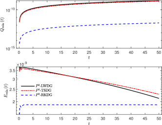
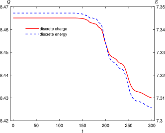
Let us further investigate the performance of the numerical schemes in the charge and energy conservations. Figure 4.1 shows the time evolution of the relative charge and energy differences defined by
with . The results show that the present three DG methods can conserve the discrete charge and the discrete energy approximately.
Finally, we test the CPU time executed by MATLAB and C++ according to the pseudo codes. The parameters are the same as those in the accuracy test except for . Tables 5 and 6 record the CPU times for different schemes by MATLAB and C++ respectively, those data are the average values of five calculations in order to reduce the error, and the output time is taken as . It is seen that when is large enough, those numerical results are consistent with the analysis in Section 3.3.
| Schemes | 100000 | 200000 | 400000 | 800000 |
|---|---|---|---|---|
| -LWDG | 4.77 | 23.07 | 92.11 | 369.73 |
| -TSDG | 4.06 | 20.41 | 82.37 | 330.87 |
| -RKDG | 3.99 | 21.21 | 85.95 | 343.80 |
| -LWDG | 8.76 | 39.68 | 158.02 | 633.73 |
| -TSDG | 7.60 | 37.57 | 150.40 | 600.27 |
| -RKDG | 7.59 | 38.62 | 155.49 | 622.40 |
| Schemes | 100000 | 200000 | 400000 | 800000 |
|---|---|---|---|---|
| -LWDG | 11.46 | 46.11 | 183.62 | 727.79 |
| -TSDG | 9.21 | 37.51 | 150.48 | 593.24 |
| -RKDG | 9.67 | 39.29 | 156.26 | 619.45 |
| -LWDG | 21.24 | 84.61 | 335.62 | 1344.08 |
| -TSDG | 19.75 | 79.00 | 314.68 | 1244.57 |
| -RKDG | 20.85 | 83.40 | 332.78 | 1324.90 |
Example 4.2 (Error history).
The -error history is investigated in this example. The NLD equation and parameters are the same as those in Example 4.1 except for and the initial condition .
Figure 4.2 shows the time evolution of the -errors for different methods from to , where we fit the curves linearly and list the resulting slopes. Relatively speaking, the RKDG methods perform better than the other two in a long time simulation. A similar result between the LWDG and RKDG methods for the linear advection problem is observed in [23].
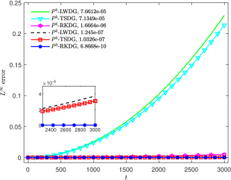
As shown in Figure 4.2, the RKDG method performs better relatively than the other two methods in a long time simulation, so we use the -RKDG method to simulate the following examples except for Example 4.4.
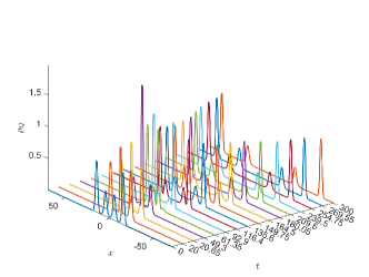
Example 4.3 (Collision).
The inelastic interaction in the binary collision and the ternary collision has been observed in [3, 40]. This example tries to observe the inelastic interaction in the quaternary collision. The initial data are taken as the linear superposition of four waves, that is, . Table 7 lists the parameters. The spatial domain is taken as , divided into cells.
Numerical results in Figure 4.3 shows the inelastic interaction in the quaternary collision and the charge decreasing property with time. The latter is consistent with Proposition 3.1.
4.2 2D case
This section investigates some 2D examples for the case of . Unless stated otherwise, we set , and the time step size is given by the following condition
with for the -LWDG method and 0.5 for the other methods.
Example 4.4 (Accuracy test).
This example tests the accuracy of our DG methods. In order to do that, we add a source term into the 2D NLD equation (2.2) as
| (4.2) |
so that the exact solutions of (4.2) can be taken as with the constant complex number , . It is the so-called method of manufactured solutions. The initial condition is taken as with , , and the exact solution being , and the spatial domain is taken as .
Tables 8-10 list the errors at and corresponding convergence rates, which are consistent with the expected.
| Schemes | error | order | error | order | |
|---|---|---|---|---|---|
| -LWDG | 40 40 | 9.1886e-03 | - | 1.9059e-02 | - |
| 80 80 | 2.3082e-03 | 1.99 | 4.7100e-03 | 2.02 | |
| 160160 | 5.7818e-04 | 2.00 | 1.1876e-03 | 1.99 | |
| 320320 | 1.4469e-04 | 2.00 | 2.9750e-04 | 2.00 | |
| -LWDG | 20 20 | 3.9147e-03 | - | 7.5917e-03 | - |
| 40 40 | 4.8257e-04 | 3.02 | 9.4199e-04 | 3.01 | |
| 80 80 | 5.9930e-05 | 3.01 | 1.1967e-04 | 2.98 | |
| 160160 | 7.4856e-06 | 3.00 | 1.5132e-05 | 2.98 | |
| -LWDG | 20 20 | 4.6905e-04 | - | 1.7709e-03 | - |
| 40 40 | 3.2684e-05 | 3.84 | 1.4145e-04 | 3.65 | |
| 80 80 | 2.1343e-06 | 3.94 | 9.8153e-06 | 3.85 | |
| 160160 | 1.4042e-07 | 3.93 | 6.2605e-07 | 3.97 |
| Schemes | error | order | error | order | |
|---|---|---|---|---|---|
| -TSDG | 40 40 | 9.1237e-03 | - | 1.8786e-02 | - |
| 80 80 | 2.2918e-03 | 1.99 | 4.5573e-03 | 2.04 | |
| 160160 | 5.7418e-04 | 2.00 | 1.1485e-03 | 1.99 | |
| 320320 | 1.4371e-04 | 2.00 | 2.8793e-04 | 2.00 | |
| -TSDG | 20 20 | 3.9203e-03 | - | 7.7629e-03 | - |
| 40 40 | 4.8322e-04 | 3.02 | 9.4513e-04 | 3.04 | |
| 80 80 | 6.0058e-05 | 3.01 | 1.2176e-04 | 2.96 | |
| 160160 | 7.4967e-06 | 3.00 | 1.5362e-05 | 2.99 | |
| -TSDG | 20 20 | 4.6357e-04 | - | 1.6581e-03 | - |
| 40 40 | 3.2458e-05 | 3.84 | 1.3339e-04 | 3.64 | |
| 80 80 | 2.1220e-06 | 3.94 | 9.3929e-06 | 3.83 | |
| 160160 | 1.3493e-07 | 3.98 | 6.0154e-07 | 3.96 |
| Schemes | error | order | error | order | |
|---|---|---|---|---|---|
| -RKDG | 40 40 | 9.1862e-03 | - | 1.8488e-02 | - |
| 80 80 | 2.2727e-03 | 2.02 | 4.2929e-03 | 2.11 | |
| 160160 | 5.6610e-04 | 2.01 | 1.0160e-03 | 2.08 | |
| 320320 | 1.4138e-04 | 2.00 | 2.4606e-04 | 2.05 | |
| -RKDG | 20 20 | 4.2264e-03 | - | 9.6981e-03 | - |
| 40 40 | 5.2404e-04 | 3.01 | 1.2033e-03 | 3.01 | |
| 80 80 | 6.5573e-05 | 3.00 | 1.4619e-04 | 3.04 | |
| 160160 | 8.1943e-06 | 3.00 | 1.8016e-05 | 3.02 | |
| -RKDG | 20 20 | 4.7686e-04 | - | 1.9168e-03 | - |
| 40 40 | 3.3019e-05 | 3.85 | 1.5175e-04 | 3.66 | |
| 80 80 | 2.1497e-06 | 3.94 | 1.0473e-05 | 3.86 | |
| 160160 | 1.3604e-07 | 3.98 | 6.6968e-07 | 3.97 |
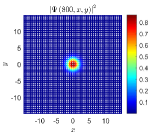
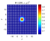
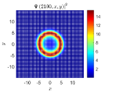
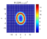
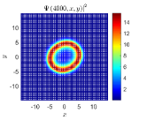
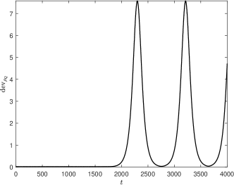
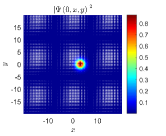
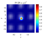
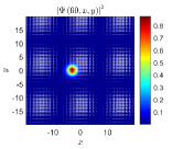
Example 4.5 (Standing wave solutions).
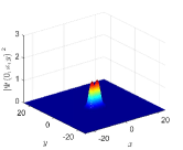
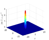
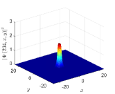
This example considers two standing wave solutions [12] of the 2D NLD equation: (i) , (ii) .
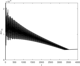
Figures 4.4 and 4.5 show the charge densities of those standing wave solutions at several different times obtained with . Figure 4.6 records the maximum deviations of the charge density defined by
We see that the charge density in the first case is almost unchanged for a very long time, while for the second one, it rotates around the center from about , and reaches the maximum amplitude at about . It is an interesting phenomenon that after a certain time, the charge density changes periodically with “circular ring-elliptical ring-circular ring”, but has not been observed in the literature.


Example 4.6 (Oscillation state).
This example investigates the interaction of two standing waves of the 2D NLD equation. The initial condition is taken as the linear superposition of two standing waves, i.e., . The computational domain is taken as .
Figure 4.7 gives the charge densities at , with . Figure 4.8 plots the charge density at with respect to . One can see that a long-lived oscillation state is observed.


Example 4.7 (Travelling wave solutions).
This example simulate two travelling wave solutions of the 2D NLD equation. The computational domain is taken as .
Figure 4.9 shows the charge densities at several different times, reflecting the motion of the travelling waves, where the first and second rows are for the cases of with and with , respectively.

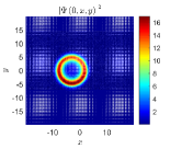
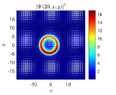
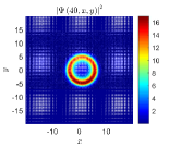
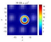
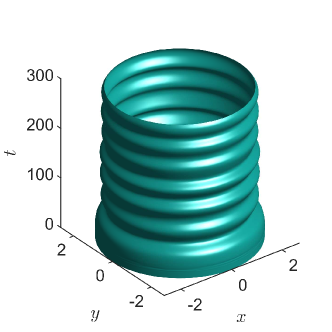
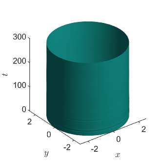
Example 4.8 (Breathing pattern).
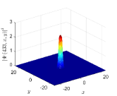
The last example investigates the influence of on the standing wave solution of the 2D NLD equation.
The left plot of Figure 4.10 shows the isosurface (with the value of 0.1) of the charge density from to with and . It presents a breathing pattern. For comparison, the right plot of Figure 4.10 gives corresponding result for the case of , where no breathing pattern is observed.
5 Conclusion
Based on the Runge-Kutta time discretization, the Lax-Wendroff type time discretization, and the two-stage fourth-order time discretization, this paper developed three high-order accurate DG methods for the 1D and 2D NLD equations with a general scalar self-interaction, denoted respectively by RKDG, LWDG and TSDG. The RKDG method used the spatial DG approximation to discretize the NLD equations and then utilized the explicit multistage Runge-Kutta time discretization for the first-order time derivatives, while the LWDG and TSDG methods, on the contrary, first gave the one-stage fourth-order Lax-Wendroff type and the two-stage fourth-order time discretizations of the NLD equations, respectively, and then discretized the first- and higher-order spatial derivatives by using the spatial DG approximation. For the 2D semi-discrete DG methods with the Lax-Friedrichs flux, we proved the stability, that is, the total charge does not increase. Moreover, those three DG methods was compared: (1) The estimation of their computational complexities in the 1D case showed that the computational complexity of the one-stage LWDG method was higher than the other two schemes. It was also verified by ous numerical experiments with MATLAB and C++. The main reason was that the LWDG method needed to calculate the high-order spatial derivatives of the solution and the nonlinear term, while the TSDG method only calculated the first-order derivatives of the nonlinear term and the RKDG method did not require to calculate the derivatives of the nonlinear term. (2) Recording the error in a long time simulation showed that the RKDG method performed relatively better than the other two methods. Several numerical examples were given to verify the above findings, and the accuracy and the conservative properties of the proposed methods. In addition, we also simulated the interaction of the 1D solitary waves and the 2D standing and travelling wave solutions. Specially, the breathing pattern was observed clearly in the case of . To conduct the 2D numerical experiments, the travelling wave solutions of the 2D NLD equation were given, according to the standing wave solutions obtained in [12] and the Lorentz transformation. Unlike the standing wave solution, the travelling wave solution was not centrosymmetric.
Acknowledgement
The second author was partially supported by the National Natural Science Foundation of China (No. 11421101).
Appendix A Calculation of and in (3.20) and (3.21)
To calculate , one needs to compute high-order (up to third-order) time derivatives of . Those time derivatives can be replaced with the spatial derivatives of , thanks to the NLD equation (3.2).
Using the definition of in (3.2) gives
| (A.1) |
where is calculated from the NLD equation (3.2) directly. Using (A.1) gives
| (A.2) |
where is calculated by using the NLD equation (3.2) as follows
| (A.3) |
Here
| (A.4) | ||||
| (A.5) | ||||
| (A.6) |
and
| (A.7) | ||||
| (A.8) | ||||
| (A.9) |
Using (A.2) further gives
| (A.10) |
where is computed from (3.2) or (A.3) as follows
| (A.11) |
Here
| (A.12) | ||||
| (A.13) | ||||
| (A.14) |
with
and
The terms and in (A.14) are calculated as follows
| (A.15) | ||||
| (A.16) |
In the above equations, , , , , , , , , , and can be obtained by (3.2), (A.3), (A.4), (A.5), (A.7), (A.8) and (A.9). Finally, substituting (A.1), (A.2) and (A.10) into Eq. (3.20) gives .
Appendix B Pseudo codes
The pseudo codes are given here for executing three 1D DG methods. The numbers in each line represent the needed amount of the corresponding operations.
Algorithm 1 Pseudo codes for -LWDG
Algorithm 2 Pseudo codes for -TSDG
Algorithm 3 Pseudo codes for -RKDG
References
- [1] D. A. Abanin, S. V. Morozov, L. A. Ponomarenko, R. V. Gorbachev, A. S. Mayorov, M. I. Katsnelson, K. Watanabe, T. Taniguchi, K. S. Novoselov, L. S. Levito, A. K. Geim, Giant nonlocality near the Dirac point in graphene, Science, 332(6027): 328–330, 2011.
- [2] A. Alvarez, Linearized Crank-Nicolson scheme for nonlinear Dirac equations, J. Comput. Phys., 99(2): 348–350, 1992.
- [3] A. Alvarez, B. Carreras, Interaction dynamics for the solitary waves of a nonlinear Dirac model, Phys. Lett. A, 86(6–7): 327–332, 1981.
- [4] A. Alvarez, P. Y. Kuo, L. Vazquez, The numerical study of a nonlinear one-dimensional Dirac equation, Appl. Math. Comput., 13(1–2): 1–15, 1983.
- [5] C. D. Anderson, The positive electron, Phys. Rev., 43(6): 491–498, 1933.
- [6] W.Z. Bao, Y.Y. Cai, X.W. Jia, J. Yin, Error estimates of numerical methods for the nonlinear Dirac equation in the nonrelativistic limit regime, Sci. China Math., 59(8): 1461–1494, 2016.
- [7] Y.Y. Cai, Y. Wang, A uniformly accurate (UA) multiscale time integrator pseudospectral method for the nonlinear Dirac equation in the nonrelativistic limit regime, ESAIM Math. Model. Numer. Anal., 52(2): 543–566, 2018.
- [8] A. H. Castro Neto, N. M. R. Peres, K. S. Novoselov, A. K. Geim, The electronic properties of graphene, Rev. Mod. Phys., 81(1): 109–162, 2009.
- [9] B. Cockburn, C.-W. Shu, TVB Runge-Kutta local projection discontinuous Galerkin finite element method for conservation laws II: General framework, Math. Comp., 52(186): 411–435, 1989.
- [10] B. Cockburn, C.-W. Shu, The Runge-Kutta discontinuous Galerkin method for conservation laws V: Multidimensional systems, J. Comput. Phys., 141(2): 199–224, 1998.
- [11] F. Cooper, A. Khare, B. Mihaila, A. Saxena, Solitary waves in the nonlinear Dirac equation with arbitrary nonlinearity, Phys. Rev. E, 82(3): 036604, 2010.
- [12] J. Cuevas-Maraver, N. Boussaïd, A. Comech, R. Lan, P. G. Kevrekidis, A. Saxena, Solitary Waves in the Nonlinear Dirac Equation, vol. 1, Chap. 4, 89–143, Cham: Springer International Publishing, 2018.
- [13] J. Cuevas-Maraver, P. G. Kevrekidis, A. Saxena, A. Comech, R. Lan, Stability of solitary waves and vortices in a 2D nonlinear Dirac model, Phys. Rev. Lett., 116(21): 214101, 2016.
- [14] F. de la Hoz, F. Vadillo, An integrating factor for nonlinear Dirac equations, Comput. Phys. Commun., 181(7): 1195–1203, 2010.
- [15] P. A. M. Dirac, The quantum theory of the electron, Proc. R. Soc. Lond. A, 117(778): 610–624, 1928.
- [16] P. A. M. Dirac, A theory of electrons and protons, Proc. R. Soc. Lond. A, 126(801): 360–365, 1930.
- [17] C. L. Fefferman, M. I. Weinstein, Honeycomb lattice potentials and Dirac points, J. Amer. Math. Soc., 25(4): 1169–1220, 2012.
- [18] F. Fillion-Gourdeau, E. Lorin, A. D. Bandrauk, Resonantly ebhanced pair production in a simple diatomic model, Phys. Rev. Lett., 110(1): 013002, 2013.
- [19] R. Finkelstein, C. Fronsdal, P. Kaus, Nonlinear spinor field, Phys. Rev., 103(5): 1571–1579, 1956.
- [20] R. Finkelstein, R. Lelevier, M. Ruderman, Nonlinear spinor fields, Phys. Rev., 83(2): 326–332, 1951.
- [21] J. D. Frutos, J. M. Sanz-serna, Split-step spectral schemes for nonlinear Dirac systems, J. Comput. Phys., 83(2): 407–423, 1989.
- [22] D.J. Gross, A. Neveu, Dynamical symmetry breaking in asymptotically free field theories, Phys. Rev. D, 10: 3235-3253, 1974.
- [23] W. Guo, J.-M. Qiu, J. Qiu, A new Lax-Wendroff discontinuous Galerkin method with superconvergence, J. Sci. Comput., 65(1): 299–326, 2015.
- [24] L. Haddad, L. Carr, The nonlinear Dirac equation in Bose-Einstein condensates: Foundation and symmetries, Physica D: Nonlinear Phenomena, 238: 1413–1421, 2009.
- [25] W. Heisenberg, Quantum theory of fields and elementary particles, Rev. Mod. Phys., 29(3): 269–278, 1957.
- [26] J. Hong, C. Li, Multi-symplectic Runge-Kutta methods for nonlinear Dirac equations, J. Comput. Phys., 211(2): 448–472, 2006.
- [27] D. D. Ivanenko, Notes to the theory of interaction via particles, Zhurn. Exp. Teoret. Fiz., 8: 260–266, 1938.
- [28] T. Lakoba, Numerical study of solitary wave stability in cubic nonlinear dirac equations in 1D, Phys. Lett. A, 382(5): 300–308, 2018.
- [29] J. Li, Z. Du, A two-stage fourth order time-accurate discretization for Lax-Wendroff type flow solvers I. Hyperbolic conservation laws, SIAM J. Sci. Comput., 38(5): A3046–A3069, 2016.
- [30] S.-C. Li, X.-G. Li, High-order compact methods for the nonlinear Dirac equation, Comput. Appl. Math., 37(5): 6483–6498, 2018.
- [31] S.-C. Li, X.-G. Li, High-order conservative schemes for the nonlinear Dirac equation, Int. J. Comput. Math., Published online, 2019. https://doi.org/10.1080/00207160.2019.1698735
- [32] S.-C. Li, X.-G. Li, F.-Y. Shi, Time-splitting methods with charge conservation for the nonlinear Dirac equation, Numer. Meth. Part. D. E., 33(5): 1582–1602, 2017.
- [33] P. Mathieu, R. Saly, Baglike solutions of a Dirac equation with fractional nonlinearity, Phys. Rev. D, 29: 2879–2883, 1984.
- [34] K. S. Novoselov, A. K. Geim, S. V. Morozov, D. Jiang, M. I. Katsnelson, I. V. Grigorieva, S. V. Dubonos, A. A. Firsov, Two-dimensional gas of massless Dirac fermions in graphene, Nature, 438(7065): 197–200, 2005.
- [35] J. Qiu, M. Dumbser, C.-W. Shu, The discontinuous Galerkin method with Lax-Wendroff type time discretizations, Comput. Methods Appl. Mech. Eng., 194(42): 4528–4543, 2005.
- [36] A. Raada, Classical nonlinear dirac field models of extended particles, in: A.O. Barut (Ed.), Quantum Theory, Groups, Fields and Particles, Springer, New York, 1983, 271-291.
- [37] B. Saha, Nonlinear spinor fields and its role in cosmology, Int. J. Theor. Phys., 51(6): 1812–1837, 2012.
- [38] S.H. Shao, N. R. Quintero, F. G. Mertens, F. Cooper, A. Khare, A. Saxena, Stability of solitary waves in the nonlinear Dirac equation with arbitrary nonlinearity, Phys. Rev. E, 90(3): 032915, 2014.
- [39] S.H. Shao, H.Z. Tang, Interaction for the solitary waves of a nonlinear Dirac model, Phys. Lett. A, 345(1–3): 119–128, 2005.
- [40] S.H. Shao, H.Z. Tang, Higher-order accurate Runge-Kutta discontinuous Galerkin methods for a nonlinear Dirac model, Discrete Cont. Dyn. B, 6(3): 623–640, 2006.
- [41] S.H. Shao, H.Z. Tang, Interaction of solitary waves with a phase shift in a nonlinear Dirac model, Commun. Comput. Phys., 3: 950–967, 2008.
- [42] C.-W. Shu, S. Osher, Efficient implementation of essentially non-oscillatory shock-capturing schemes, J. Comput. Phys., 77(2): 439–471, 1988.
- [43] M. Soler, Classical, stable, nonlinear spinor field with positive rest energy, Phys. Rev. D, 1(10): 2766–2769, 1970.
- [44] W. E. Thirring, A soluble relativistic field theory, Ann. Phys., 3(1): 91–112, 1958.
- [45] H. Wang, H.Z. Tang, An efficient adaptive mesh redistribution method for a non-linear Dirac equation, J. Comput. Phys., 222(1): 176–193, 2007.
- [46] H. Weyl, A remark on the coupling of gravitation and electron, Phys. Rev., 77: 699–701, 1950.
- [47] Z.Q. Wang, B.Y. Guo, Modified Legendre rational spectral method for the whole line, J. Comput. Math., 22: 457–474, 2004.
- [48] J. Xu, S.H. Shao, H.Z. Tang, Numerical methods for nonlinear Dirac equation, J. Comput. Phys., 245: 131–149, 2013.
- [49] J. Xu, S.H. Shao, H.Z. Tang, D. Wei, Multi-hump solitary waves of a nonlinear Dirac equation, Commun. Math. Sci., 13(3): 1219–1242, 2015.
- [50] Y. Xu, C.-W. Shu, Local discontinuous Galerkin methods for nonlinear Schrödinger equations, J. Comput. Phys., 205(1): 72–97, 2005.
- [51] Y.H. Yuan, H.Z. Tang, Two-stage fourth-order accurate time discretizations for 1D and 2D special relaticistic hydrodynamics, J. Comput. Math., 38(5): 768–796, 2020.
- [52] Y.H. Yuan, H.Z. Tang, On the explicit two-stage fourth-order accurate time discretizations, arXiv: 2007.02488, Jul. 2020.