Learning in the Wild with Incremental Skeptical Gaussian Processes

Abstract

The ability to learn from human supervision is fundamental for personal assistants and other interactive applications of AI. Two central challenges for deploying interactive learners in the wild are the unreliable nature of the supervision and the varying complexity of the prediction task. We address a simple but representative setting, incremental classification in the wild, where the supervision is noisy and the number of classes grows over time. In order to tackle this task, we propose a redesign of skeptical learning centered around Gaussian Processes (GPs). Skeptical learning is a recent interactive strategy in which, if the machine is sufficiently confident that an example is mislabeled, it asks the annotator to reconsider her feedback. In many cases, this is often enough to obtain clean supervision. Our redesign, dubbed isgp, leverages the uncertainty estimates supplied by GPs to better allocate labeling and contradiction queries, especially in the presence of noise. Our experiments on synthetic and real-world data show that, as a result, while the original formulation of skeptical learning produces over-confident models that can fail completely in the wild, isgp works well at varying levels of noise and as new classes are observed.

1 Introduction

Imagine a handheld personal assistant that provides guidance to an end-user. In order to give useful, timely suggestions (like “please take your insulin”), the agent must be aware of the user’s context, for instance where she is (“at home”), what she is doing (“eating cake”), and with whom (“alone”). The machine must infer this information from a stream of sensor readings (e.g., GPS coordinates, nearby Bluetooth devices), with the caveat that the target classes are user-specific (e.g., this user’s home is not another user’s home) and thus that the label vocabulary must be acquired from the user herself. Moreover, as the user visits new places and engages in new activities, the vocabulary changes. This simple example shows that, in order to be successful outside of the lab Dietterich (2017), AI agents must adapt to the changing conditions of the real world and to their end-users.

We study these challenges in a simplified but non-trivial setting, interactive classification in the wild, where an interactive learner requests labels from an end-user and the number of classes grows with time. A fundamental issue in this setting is that end-users often provide unreliable supervision Tourangeau et al. (2000); West and Sinibaldi (2013); Zeni et al. (2019). This is especially problematic in the wild, as noisy labels may fool the machine into being under- or over-confident and into acquiring non-existent classes.

We address these issues by proposing Incremental Skeptical Gaussian Processes (isgp), a redesign of skeptical learning Zeni et al. (2019) tailored for learning in the wild. In skeptical learning (SKL), if the interactive learner is confident that a newly obtained example is mislabeled, it immediately asks the annotator to reconsider her feedback. In stark contrast to other noise handling alternatives, SKL is designed specifically to retrieve the clean label from the annotator.

isgp improves SKL in four important ways. First, isgp builds on Gaussian Processes (GPs) Williams and Rasmussen (2006). Thanks to their explicit uncertainty estimates, GPs prevent pathological cases in which an overconfident learner 1) refuses to request the label of instances far from the training set, thus failing to learn, and 2) continuously challenges the user regardless of her past performance, estranging her. Second, isgp makes use of the model’s uncertainty to determine whether to be skeptical or credulous, while SKL uses an inflexible strategy that relies on the number of observed examples only. Third, while SKL relies on several hard-to-choose hyper-parameters, isgp makes use of a simple and robust algorithm that works well even without fine-tuning. Last, isgp makes use of incremental learning techniques for improved scalability Lütz et al. (2013).

Summarizing, we: 1) Introduce interactive classification in the wild, a novel form of interactive learning in which there is as substantial amount of labelling noise and new classes are observed over time; 2) Develop isgp, a simple and robust redesign of skeptical learning that leverages exact uncertainty estimates to appropriately allocate queries to the user and avoids over-confident models even in the presence of noise; 3) Showcase the advantages of isgp – in terms of query budget allocation, prediction quality and efficiency – on a controlled synthetic task and on a real-world task.

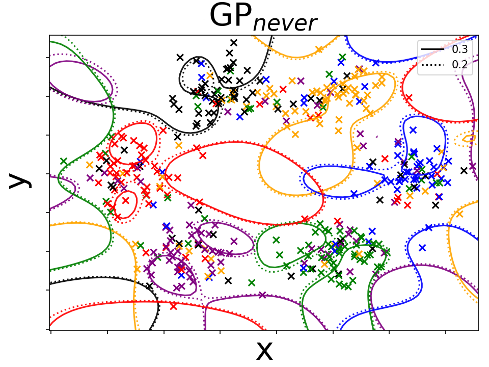
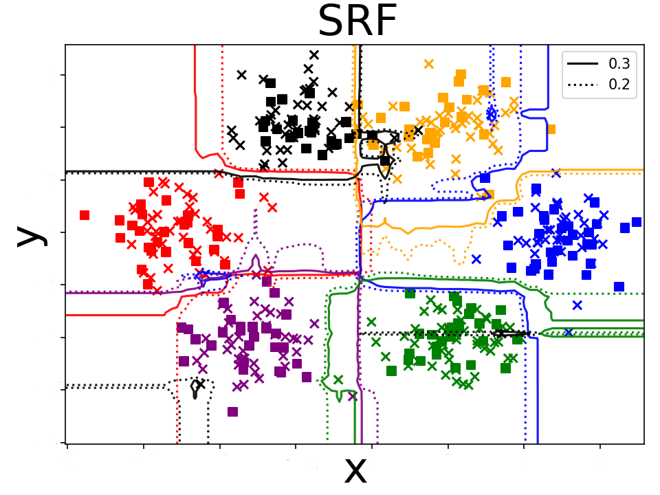
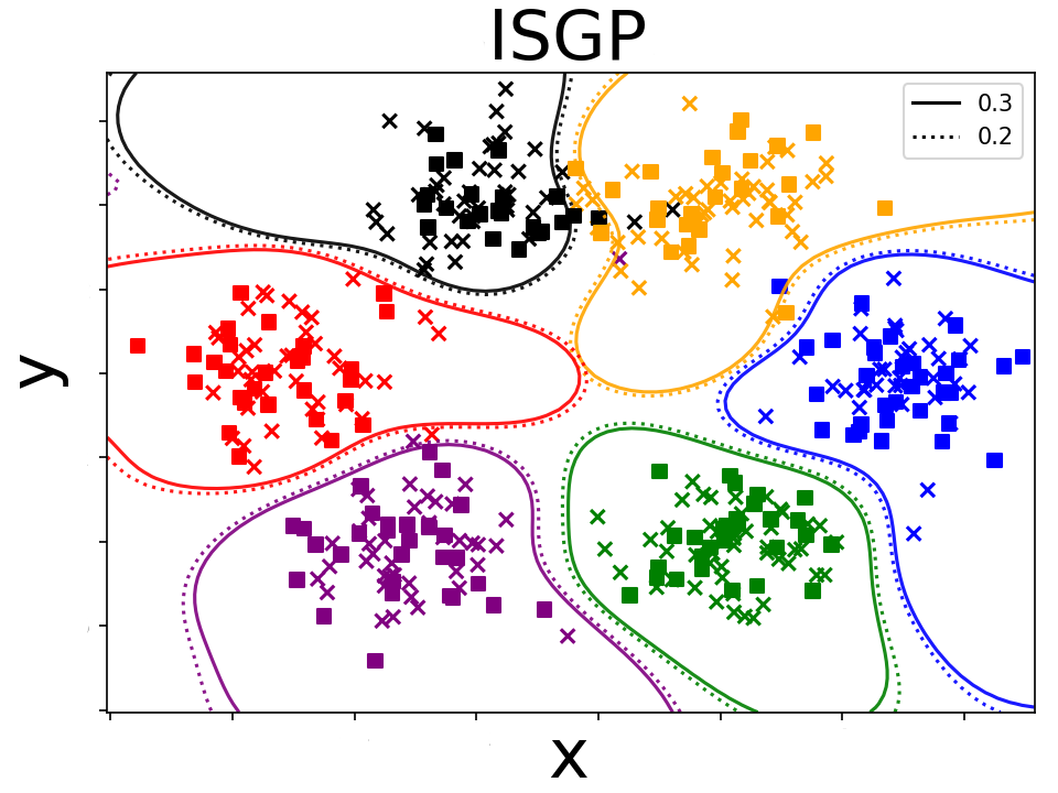
Figure 1: Illustration of isgp on a 2D synthetic data set with six normally-distributed classes (in color) and noisy labels (corrupted at random with probability $0.4$). The outlines enclose regions with high predictive probability (solid $\geq 0.3$, dashed $\geq 0.2$). Crosses and boxes are noisy examples; boxes have been cleaned by skeptical learning. From the left: regular GP, skeptical learning, and isgp. Best viewed in color.

2 Incremental Classification in the Wild

Interactive classification in the wild (ICW) is a sequential prediction task: in each round $t=1,2,\ldots,$ the learner receives an instance $x_{t}\in\mathcal{X}$ (e.g., a vector of sensor readings) and outputs a prediction $\hat{y}_{t}\in\mathcal{Y}$ (e.g., the user’s location). The learner is also free to query a human annotator – usually the end-user herself – for the ground-truth label $y_{t}\in\mathcal{Y}$ (e.g., the true location). The goal of the learner is to acquire a good predictor while keeping the number of queries at a minimum, not to overload the annotator.

Two features make ICW unique: the amount of label noise and the presence of task shift. Label noise follows from the fact that human annotators are often subject to momentary inattention and may fail to understand the query Zeni et al. (2019). The label $\tilde{y}_{t}$ fed back by the annotator is thus often wrong, i.e., $\tilde{y}_{t}\neq y_{t}$. Failure to handle noise can bloat the model and affect its accuracy Frénay and Verleysen (2014). Label noise is especially troublesome in ICW, as it can fool the model into being under- or over-confident. This in turn makes it difficult to identify informative instances and properly allocate labeling budget.

By task shift we mean that newly received instances may belong to new and unanticipated classes. For this reason, we distinguish between the complete but unobserved set of classes $\mathcal{Y}\subseteq\mathbb{N}$ and the classes observed up to iteration $t$, that is $\mathcal{Y}_{t}\subseteq\mathcal{Y}$. Hence, $y_{t}$ belongs to $\mathcal{Y}$, $\tilde{y}_{t}$ to $\mathcal{Y}_{t}$, and $\hat{y}_{t}$ to $\mathcal{Y}_{t-1}$. To keep the task manageable, we assume that previously observed classes remain valid, i.e, $\mathcal{Y}_{t}\subseteq\mathcal{Y}_{t+1}$ for all $t$. In our personal aid example, this would imply that, for instance, the user’s home remains the same over time. This is a reasonable assumption so long as the agent’s lifetime is not too long. A study of other forms of task shift is left to future work.

3 Skeptical Learning

Skeptical learning (SKL) is a noise handling strategy designed for interactive learning Zeni et al. (2019). The idea behind SKL is simple: rather than blindly accepting the annotator’s supervision, a skeptical learner challenges the annotator about any suspicious examples it receives. In contrast with standard strategies for handling noise, like using robust models or discarding anomalies Frénay and Verleysen (2014), SKL aims at recovering the ground-truth.

In skeptical learning, an example is deemed suspicious if the learner is confident that the model’s prediction is right and that the user’s annotation is wrong. This requires the learner to assign a confidence level to its own predictions and to the user’s annotations. SKL estimates these confidences using two separate heuristics. The confidence in the model is estimated using a combination of training set size and confidence reported by the model. The confidence in the user is based on the number of user mistakes spotted during past interaction rounds. Both estimates are quite crude. See Zeni et al. (2019) for more details.

The original formulation of skeptical learning is not a good fit for ICW. First and foremost, SKL is based on random forests (RFs), which are robust to noise but also notoriously over-confident. This can be clearly seen in Figure 1: the RF in the middle plot is very confident even far away from the training set. This is a major issue, as over-confident predictors may stubbornly refuse to query novel and informative instances, compromising learning, and may keep challenging the user regardless of her past performance, overloading and estranging her. In addition, SKL structures learning into three stages: initially, the machine always requests supervision and never contradicts the user; once the model is confident enough, it begins to challenge the user; finally, the model begins to actively request for labels. This partially avoids over-confidence by requesting extra labels. This strategy fails in the wild, as new classes appear even in later learning stages, in which over-confident models may refuse to request supervision for them. This occurs frequently in our experiments. Two other issues are that SKL requires to choose several hyper-parameters (like $\theta$, which controls when to transition between stages), which is non-trivial in interactive settings, and that it retrains the RF from scratch in each iteration.

4 Skeptical Learning in the Wild

isgp is a redesign of skeptical learning based on Gaussian Processes (GPs) that avoids over-confident predictors and handles label noise. GPs are a natural choice in learning tasks like active learning Kapoor et al. (2007); Rodrigues et al. (2014), online bandits Srinivas et al. (2012), and preference elicitation Guo et al. (2010), in which uncertainty estimates help to guide the interaction with the user. Our key observation is that skeptical learning is another such application.

4.1 Gaussian Processes

Gaussian Processes (GPs) Williams and Rasmussen (2006) are non-parametric distributions over functions $f:\mathcal{X}\to\mathbb{R}$. A GP is entirely specified by a mean function $\mu(x)$ and a covariance function $k(x,x^{\prime})$. The latter encodes structural assumptions about the functions modeled by the GP and can be implemented with any kernel function. When no evidence is given, it can be assumed w.l.o.g. that $\mu(x)\equiv 0$. Bayesian inference, that is, conditioning a GP on examples, produces another GP whose mean and covariance functions can be written in closed form. Letting $\bm{\mathrm{x}}_{t}=(x_{1},\ldots,x_{t})^{\top}$ be the instances received so far and $\bm{\mathrm{y}}_{t}=(y_{1},\ldots,y_{t})^{\top}$ their “scores” $y_{t}=f(x_{t})$ (possibly perturbed by Gaussian noise), the mean and covariance functions conditioned on $(\bm{\mathrm{x}}_{t},\bm{\mathrm{y}}_{t})$ are:

$$\mu_{t}(x) \;=\bm{\mathrm{k}}_{t}(x)^{\top}\Gamma_{t}\bm{\mathrm{y}}_{t}$$ (1)

$$k_{t}(x,x^{\prime}) \;=k(x,x^{\prime})-\bm{\mathrm{k}}_{t}(x)^{\top}\Gamma_{t}\bm{\mathrm{k}}_{t}(x^{\prime})+\rho^{2}$$ (2)

Here we used $\bm{\mathrm{k}}_{t}(x)=(k(x_{1},x),\ldots,k(x_{t},x))^{\top}$, $K_{t}=[k(x,x^{\prime})\,:\,x,x^{\prime}\in\bm{\mathrm{x}}_{t}]$, $\Gamma_{t}=(K_{t}+\rho^{2}I)^{-1}$, and $\rho$ a smoothing parameter that models noise. Given a GP with parameters $(\mu,k)$ and $x$, the value of $f(x)$ is normally distributed with mean $\mu(x)$ and variance $k(x,x)$. Hence, the probability that $f(x)$ is non-negative is:

$$\textstyle\mathbb{P}(f(x)\geq 0\,|\,x)=\Phi\left(\frac{\mu(x)}{\sigma(x)}\right)$$ (3)

where $\Phi$ denotes the cdf of a standard normal distribution and $\sigma(x)=\sqrt{k(x,x)}$. This quantity is often used in classification tasks to model the probability of the positive class, that is, $\mathbb{P}(1\,|\,x)=\mathbb{P}(f(x)\geq 0\,|\,x)$, see Kapoor et al. (2007).

4.2 Incremental Multi-class GPs

Incremental multi-class GPs (IMGPs) generalize Gaussian Processes to multi-class classification Lütz et al. (2013). An IMGP can be viewed as a collection of GPs, one for each observed class $\ell\in\mathcal{Y}_{t}$, which share the same precision matrix $\Gamma_{t}$ but have separate label vectors $\bm{\mathrm{y}}_{\ell,t}$. The label vectors use a one-versus-all encoding: an element of $\bm{\mathrm{y}}_{\ell,t}$ is $1$ if the label of the corresponding example is $\ell$ and $0$ otherwise. The posterior mean function of the $\ell$-th GP is:

$$\mu_{\ell,t}(x) \;=\bm{\mathrm{k}}_{t}(x)^{\top}\Gamma_{t}\bm{\mathrm{y}}_{\ell,t}$$ (4)

Since the covariance function does not depend on the labels, it remains the same as in Eq. 2. The multi-class posterior is obtained by combining the GP posteriors with a soft-max:

$$\textstyle\mathbb{P}(\ell\,|\,x_{t})=\frac{1}{Z}\exp\mathbb{P}_{\ell}(1\,|\,x_{t}),\;Z=\sum_{\ell^{\prime}}\exp\mathbb{P}_{\ell^{\prime}}(1\,|\,x_{t})$$ (5)

Here $\mathbb{P}_{\ell}(1\,|\,x_{t})$ is the posterior of the $\ell$-th GP (Eq. (3)) and $Z$ is a normalization factor.

IMGPs offer two major advantages. First, in IMGPs the predictive variance is guaranteed to increase with the distance from the training set, as illustrated by Figure 1 (right). This prevents IMGPs from being over-confident about classes and instances that differ significantly from its previous experience, a key feature when learning in the wild. Another benefit is that IMGPs support incremental updates, i.e., in each iteration the updated precision matrix $\Gamma_{t+1}$ is computed from $\Gamma_{t}$ by exploiting the matrix-inversion lemma, without any matrix inversion Lütz et al. (2013). This makes IMGPs scale much better than non-incremental learners and GPs; see Section 4.4 for a discussion.

Algorithm 1 Pseudo-code of isgp. $\mathcal{Y}_{0}$ is provided as input. All branches are stochastic, see the relevant equations.

1:for $t=1,2,\ldots$ do

2:     receive $x_{t}$

3:     $\hat{y}_{t}\leftarrow\operatorname*{argmax}_{y\in\mathcal{Y}_{t-1}}\;\mu_{y}(x_{t})$ $\triangleright$ Eq. (6)

4:     if uncertain about $\hat{y}_{t}$ then $\triangleright$ Eq. (7)

5:         request label, receive $\tilde{y}_{t}$

6:         if skeptical about $\tilde{y}_{t}$ then $\triangleright$ Eq. (8)

7:              challenge user with $\hat{y}_{t}$, receive $y^{\prime}_{t}$

8:         else

9:              $y^{\prime}_{t}\leftarrow\tilde{y}_{t}$          

10:         add $(x_{t},y^{\prime}_{t})$ to data set and update IMGP

11:         $\mathcal{Y}_{t}\leftarrow\mathcal{Y}_{t-1}\cup\{y^{\prime}_{t}\}$      

4.3 Incremental Skeptical Gaussian Processes

We are now ready to present isgp; the pseudo-code is listed in Algorithm 1. In each iteration $t$, the learner receives an instance $x_{t}$ and predicts the most likely label (line 3):

$$\textstyle\hat{y}_{t} \textstyle=\operatorname*{argmax}_{\ell}\mathbb{P}(\ell\,|\,x_{t})=\operatorname*{argmax}_{\ell}\frac{1}{Z}\exp\mathbb{P}_{\ell}(1\,|\,x_{t})$$

$$\textstyle=\operatorname*{argmax}_{\ell}\Phi\left(\frac{\mu_{\ell,t}(x)}{\sigma_{t}(x)}\right)=\operatorname*{argmax}_{\ell}\mu_{\ell,t}(x_{t})$$ (6)

where $\ell\in\mathcal{Y}_{t-1}$. The last step holds because $\Phi$ is monotonically increasing and $\sigma_{t}(x)$ does not depend on $\ell$.

At this point, isgp has to decide whether to request the label of $x_{t}$ (line 4). In line with approaches to selective sampling Cesa-Bianchi et al. (2006); Beygelzimer et al. (2009), isgp prioritizes requesting the labels of uncertain instances, as these are more likely to impact the model. This also limits the labeling cost as the model improves. Intuitively, $x_{t}$ is uncertain if either $\mu_{\hat{y}_{t}}(x_{t})$ is small or $\sigma_{t}(x_{t})$ is large; in either case, Eq. (3) ensures that $P_{\hat{y}_{t}}(1\,|\,x_{t})$ is small. Hence, isgp queries the annotator with probability $\mathbb{P}_{\hat{y}_{t}}(0\,|\,x_{t})$. This is achieved by sampling $a_{t}$ from a Bernoulli distribution with parameter $\alpha_{t}$, defined as:

$$\textstyle\alpha_{t} =\mathbb{P}_{\hat{y}_{t}}(f(x_{t})\leq 0\,|\,x_{t})=1-\Phi\left(\mu_{\hat{y}_{t},t}(x_{t})/\sigma_{t}(x_{t})\right)$$ (7)

and querying the user if $a_{t}=1$. The choice is randomized so to prevent isgp from trusting the model too much, which is problematic, especially during the first rounds of learning. Randomization is a key ingredient in online learning and selective sampling, cf. Cesa-Bianchi et al. (2006).

If the check succeeds, isgp has to decide whether to challenge the user’s label (line 6). If the user and the machine agree on the label, the probability of challenging the user should be small; we set it to zero, for simplicity. Otherwise, it should increase with $\mathbb{P}_{\hat{y}_{t}}(1\,|\,x_{t})$ and decrease with $\mathbb{P}_{\tilde{y}_{t}}(1\,|\,x_{t})$. Since these probabilities come from different GPs, a direct comparison is not straightforward. In order to facilitate this, isgp treats the GPs as if they were independent. Under this modeling assumption, letting $f_{\ell}$ be a sample from the $\ell$-th GP, $\mathbb{P}(f_{\hat{y}_{t}}(x_{t})\geq f_{\tilde{y}_{t}}(x_{t}))$ is a normal distribution with mean $\delta_{t}(x)=\mu_{\hat{y}_{t}}(x)-\mu_{\tilde{y}_{t}}(x)$ and variance $\sigma_{t}(x)$. isgp determines whether to challenge the user by sampling from a Bernoulli with parameter $\gamma_{t}$:

$$\textstyle\gamma_{t} =\mathbb{P}(f_{\hat{y}_{t}}(x_{t})-f_{\tilde{y}_{t}}(x_{t})\geq 0)=\Phi\left(\delta_{t}(x_{t})/\sigma_{t}(x_{t})\right)$$ (8)

This is analogous to the case of active queries discussed above. Despite relying on an (admittedly strong) modeling assumption, this strategy worked well in our experiments.

Once confronted by the learner, the user replies with a potentially cleaned label $y^{\prime}_{t}$. As in the original formulation of SKL Zeni et al. (2019), this label is never contested by isgp. The reason is that in our target applications the user is collaborative and label noise is mostly due to temporary inattention. Lastly, in line (10) the model is updated using the consensus example $(x_{t},y^{\prime}_{t})$ and the loop repeats.

4.4 Advantages and Limitations

isgp improves on the original formulation of skeptical learning Zeni et al. (2019) in several ways. A major benefit is that IMGPs are never over-confident in regions far away from the training set. This facilitates allocating the query budget and avoids pathological behaviors. Our empirical analysis shows that the original formulation has no such guarantees. isgp is also simpler. isgp uses the IMGP itself to model the confidence in the annotator’s label, whereas the original implementation relies on a separate model trained heuristically. Also, learning is not heuristically split into stages and only two hyper-parameters are needed, namely $k$ and $\rho$. Since hyper-parameters are hard to tune properly in interactive tasks, this is a substantial advantage. The net effect is that isgp performs better and more consistently.

A well-known weakness of GPs is their limited scalability, due to the need of storing all past examples and of performing a matrix inversion during model updates. The latter is avoided here by using incremental updates, which reduce the per-iteration cost from $O(t^{3})$ to $O(t^{2})$. This is enough for isgp to run substantially faster than the original implementation of SKL and to handle weeks or months of interaction with no loss of reactivity, as shown by our real-world experiment. Sparse GP techniques can speed up isgp even further Quiñonero-Candela and Rasmussen (2005). Of course, GPs are not immediately applicable to lifelong tasks: these will require different (online) learning techniques. However, lifelong classification is beyond the scope of this paper.

Another limitation of isgp is that the active and skeptical checks (that is, Eqs. (7) and (8)) rely on the GP of the predicted class only. The active check can be easily adapted to use information from all classes known to the IMGP by replacing $\mathbb{P}_{\ell}(1\,|\,x_{t})$ with $\mathbb{P}(\ell\,|\,x_{t})$. An adaptation of the skeptical check, however, is non-trivial and left to a future work. In practice, this does not seem to be an issue, as isgp works much better than the original implementation of SKL.

5 Experiments

We investigate the following research questions:

Q1

Does isgp output better predictions than the original formulation of skeptical learning?

Q2

Does isgp correctly identify mislabeled examples?

Q3

Does isgp scale better than skeptical learning?

In order to address these questions, we implemented isgp using Python 3 and compared it against three alternatives on a synthetic and a real-world data set. The competitors are the original implementation of SKL Zeni et al. (2019) based on random forests, denoted srf, and two active IMGP baselines that never and always challenge the user, dubbed $\textsc{gp}_{\text{never}}$ and $\textsc{gp}_{\text{always}}$, respectively. The experiments were run on a computer with a 2.2 GHz processor and 16 GiB of memory. The code and experimental setup can be downloaded from: gitlab.com/abonte/incremental-skeptical-gp.

5.1 Synthetic Experiment

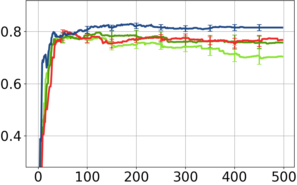
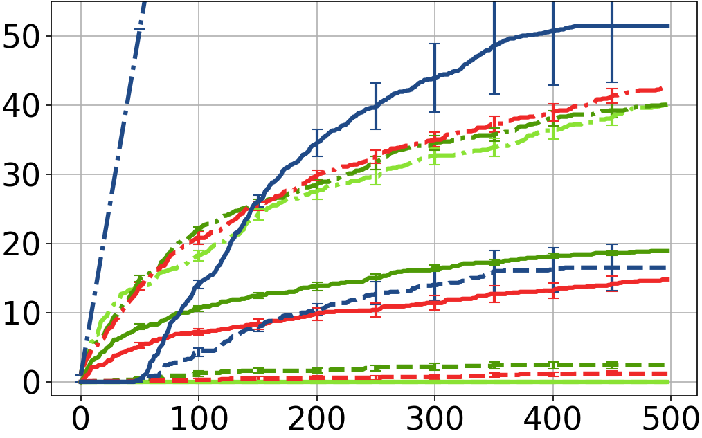
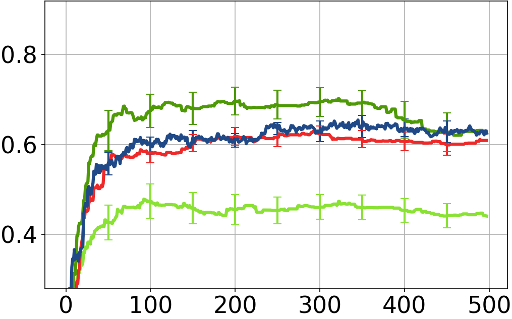
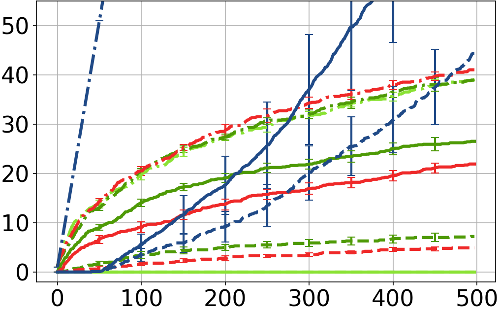
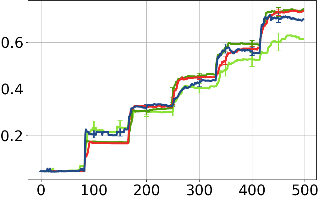
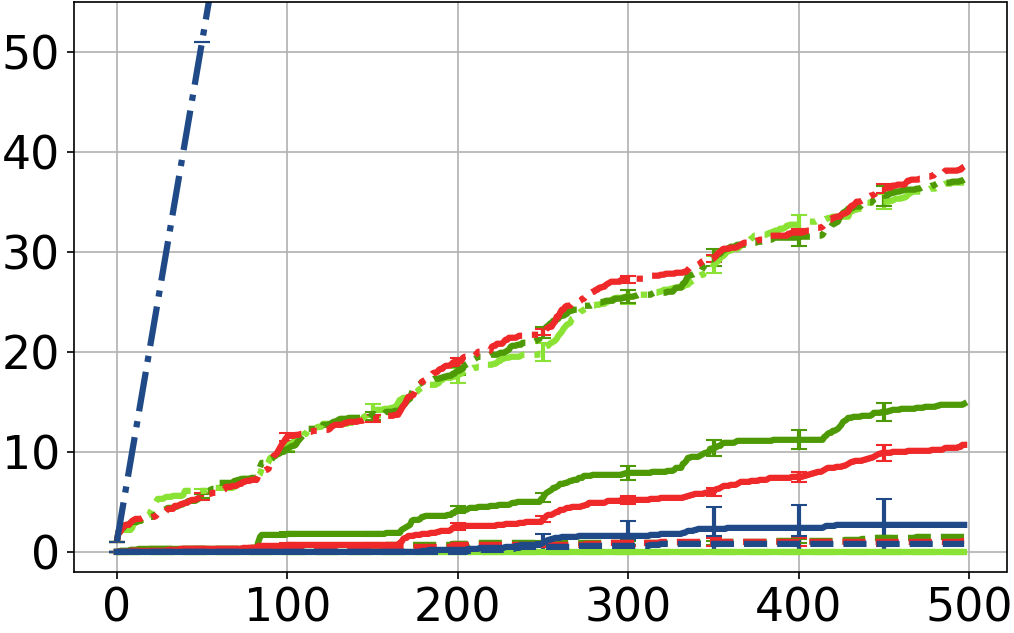
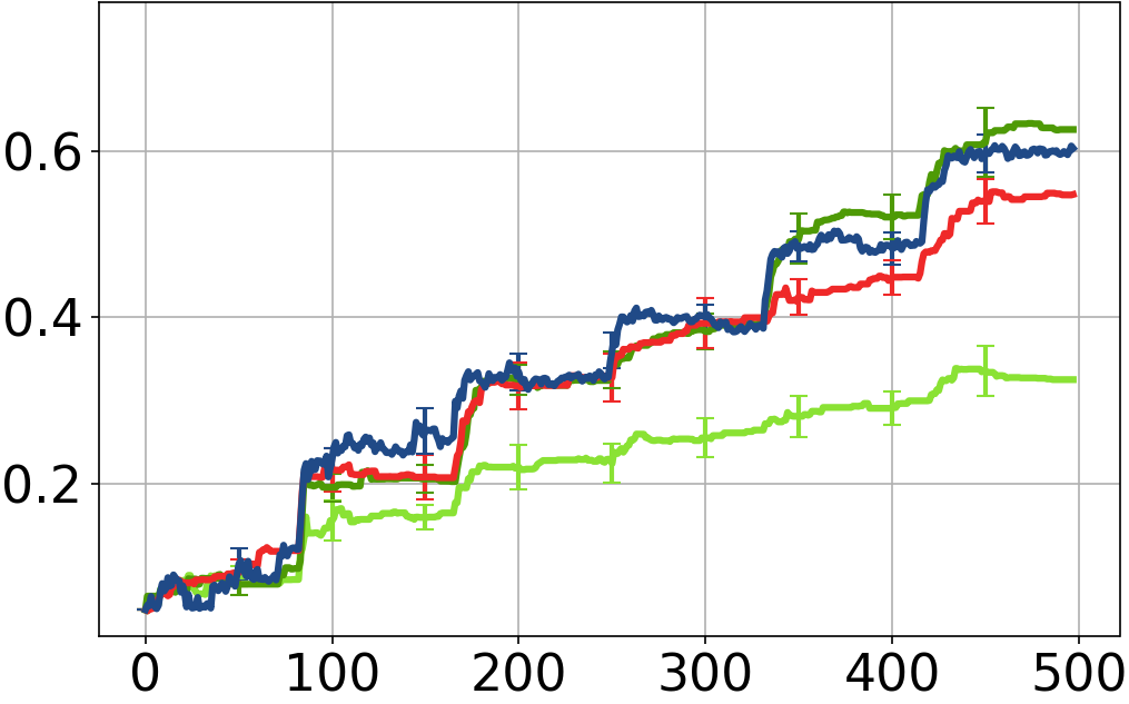
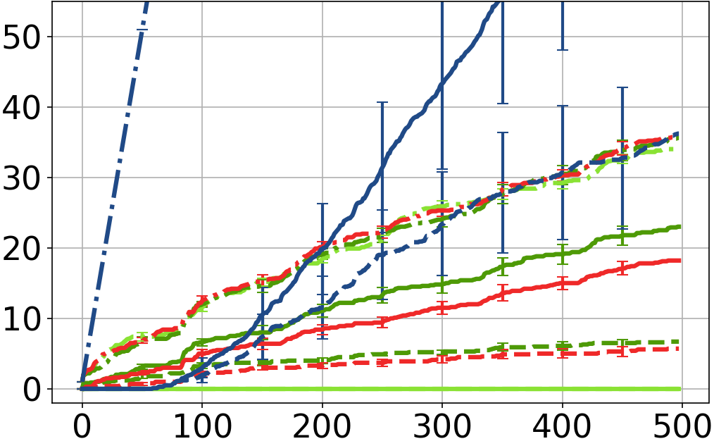
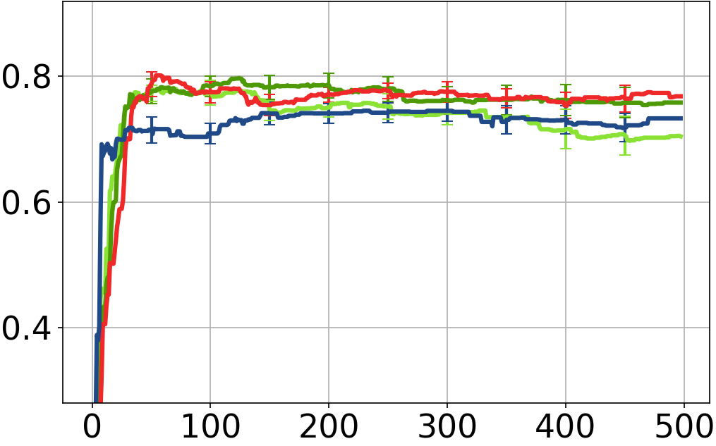
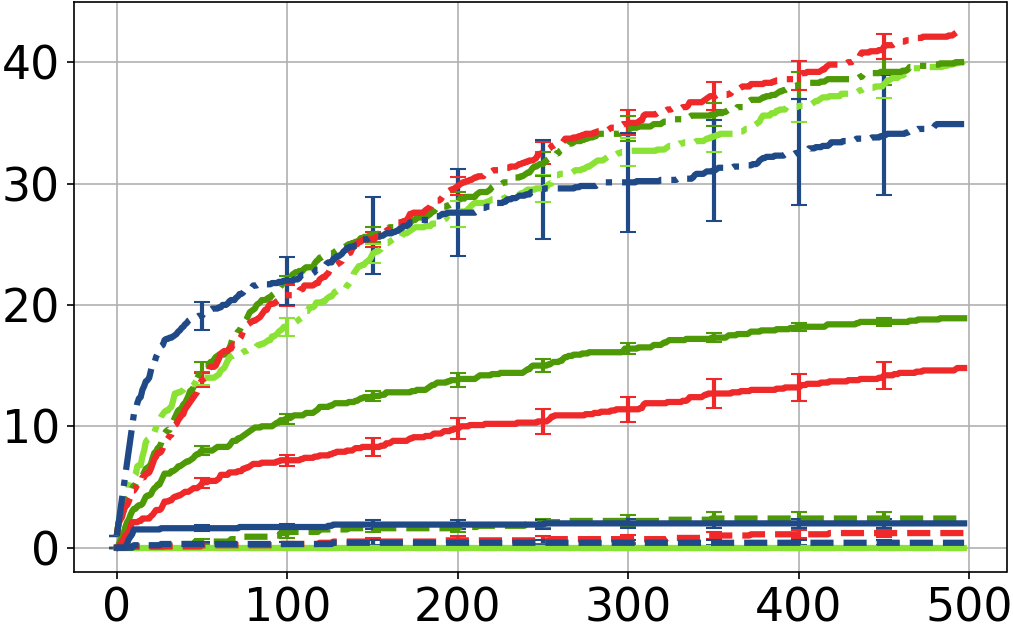
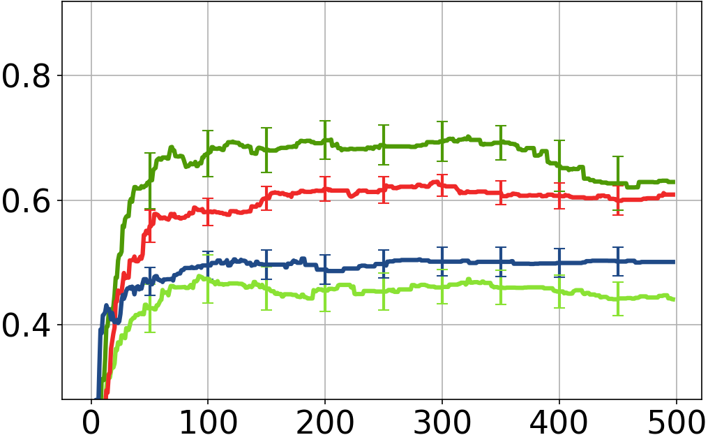
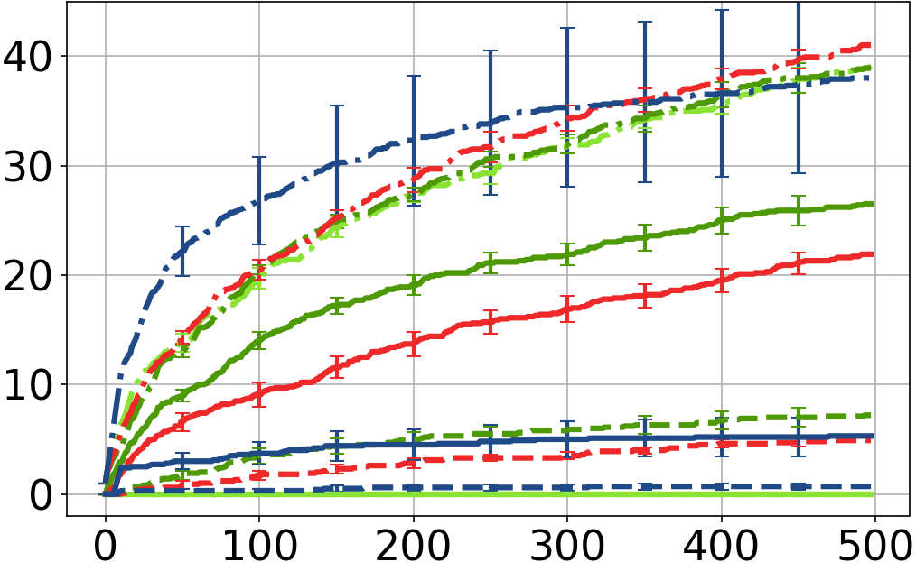
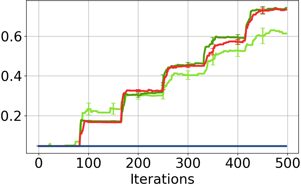
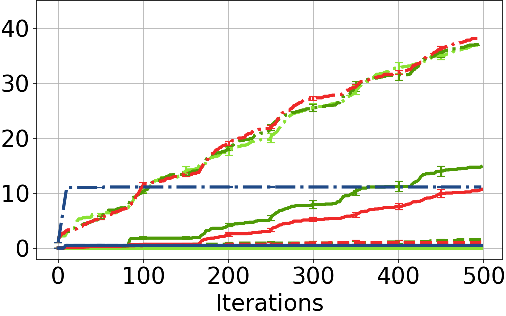
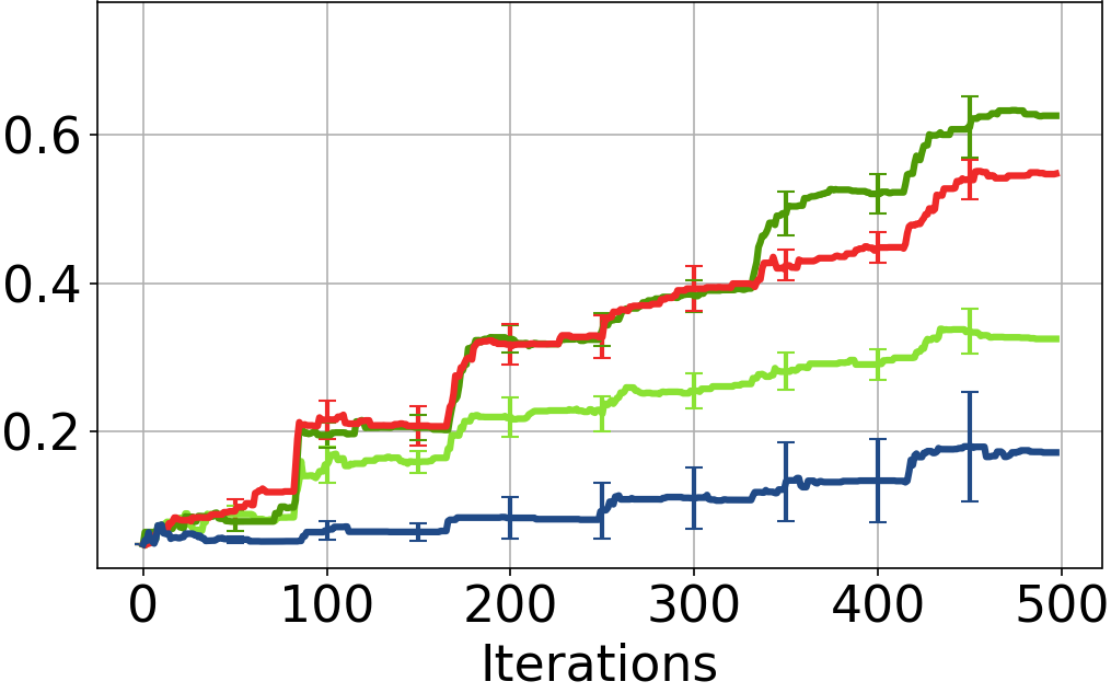
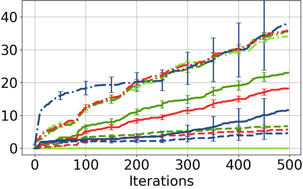
Figure 2: Results on synthetic data. The two leftmost columns report the $F_{1}$ and # of labeling and contradiction queries (bars indicate the std. err.) for $10\%$ noise; rightmost columns do the same for $40\%$ noise. Top two rows : srf tuned to match $F_{1}$ of isgp. Bottom two rows: srf tuned to match # of queries of isgp (and forced to query at least $10$ labels). Odd/even rows are random/sequential clusters, respectively.

As a first experiment, we ran all methods on a synthetic data set with six classes, similar to Figure 1: 100 instances were sampled from six 2D normal distributions, one for each class, with different means and identical standard deviations (namely $1.5$). As usual in active learning, the annotator’s responses are simulated by an oracle. Our oracle replies to labeling queries with a wrong label $\eta\%$ of the time. We experimented with a low- ($\eta=10$) and a high-noise regime ($\eta=40$). (Notice that $40\%$ noise rate is very high: $50\%$ is the limit for learnability in binary classification Angluin and Laird (1988).) While in Zeni et al. (2019) the oracle always replies to contradiction queries with the correct label, our oracle answers with a wrong label $\eta\%$ of the time (unless the label being contested is correct, in which case no mistake is possible). This is meant to better capture the behavior of human annotators, as the answer to contradiction queries can be incorrect. Results obtained using the original oracle are not substantially different from the ones below.

All results are 10-fold cross validated. For each fold, training examples are supplied in a fixed order to all methods. The order has a noticeable impact on performance, so we studied two alternatives: a) instances chosen uniformly at random; b) instances chosen randomly from sequential clusters (red, then blue, etc.). This captures task shift, i.e., increasing number of classes. $\mathcal{Y}_{0}$ matches the first example provided. All GP learners used a squared exponential kernel with a length scale of $2$ and $\rho=10^{-8}$, without any optimization. The number of trees of srf was set to $100$. The methods were evaluated based on their $F_{1}$ score and query budget usage. For simplicity, the cost of skeptical queries was assumed to be similar to that of labeling queries.

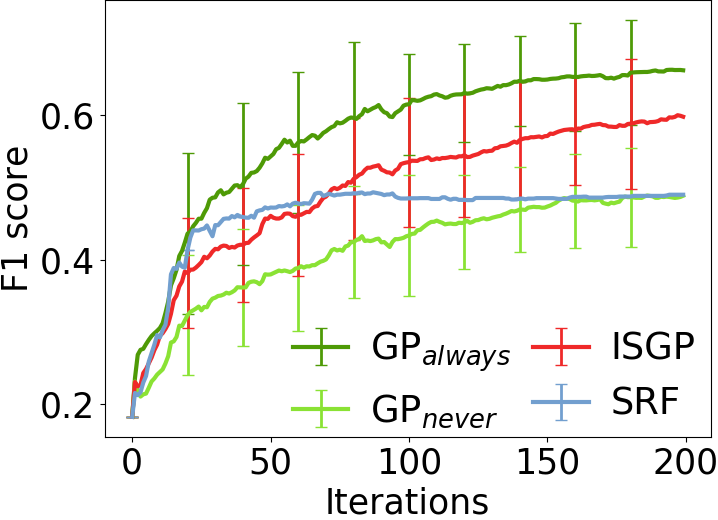
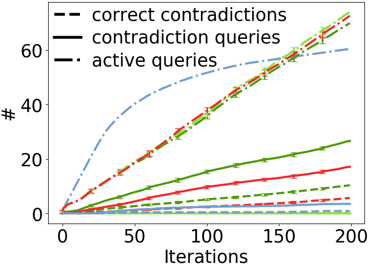
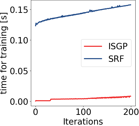
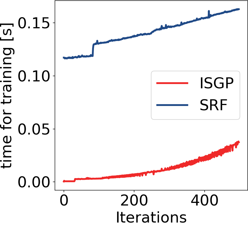
Figure 3: Results on location prediction. Left to right: $F_{1}$ score, # of queries (cumulative), and run-time (not cumulative) as learning proceeds on real-world and synthetic dataset (the training step is performed at each iteration).

The cross-validated results can be viewed in Figure 2. The plots show the $F_{1}$ score on the left-out fold and the cumulative number of queries made (dash-dot line: active queries; solid line: contradiction queries; dashed line: contradiction queries that uncovered an actual mistake). The two leftmost columns report the performance of all methods at $\eta=10\%$ noise, the rightmost columns at $40\%$. In order to enable a fair comparison, we tuned srf to either match the $F_{1}$ score of isgp or its query budget utilization. This was achieved by tuning the hyper-parameter $\theta$ of srf, which controls the length of the training and refinement stages of srf, cf. Section 3: the longer the stages, the better the estimates acquired by the random forest but the worse the query usage. These two settings are illustrated by the top two and bottom two rows of Figure 2, respectively. Finally, odd rows refer to random instance selection order, even rows to sequential order.

srf worked well only in the low-noise, random order case (left columns, first row). Here, it managed to outperform our method by about 5%. This setting, however, is not very representative of ICW, as the user is quite consistent and examples from all classes are quickly obtained. In all other cases, srf fails completely. Two trends are clearly visible. If tasked with reaching the $F_{1}$ score of isgp, srf tends to request the label of all new instances: the blue curve increases linearly beyond the plot $y$ range. This is because the value of $\theta$ needed to reach a high enough $F_{1}$ score also forces srf to remain in refine and train stage for most iterations. On the other hand, if the query budget is limited (bottom two rows), srf quickly becomes over-confident and refuses to query the user. This is especially troublesome with task shift (bottom row), as the random forest becomes confident after seeing examples from mostly one class, leading to abysmal performance.

Our method does considerably better. Most importantly, isgp does not suffer from pathological behavior and performs consistently across the board. The $F_{1}$ score typically increases with the number of queries made, even in the high-noise scenarios, while querying is not too aggressive – definitely not as aggressive as srf. The $F_{1}$ and query curves also show much lower variance compared to srf in most cases, as shown by the narrower error bars. It is easy to see that isgp usually achieves $F_{1}$ score almost indistinguishable (in low-noise conditions, left two columns) or close (high-noise, right columns) to the $F_{1}$ of $\textsc{gp}_{\text{always}}$ with a comparable number of active queries and a smaller number of skeptical ones. Moreover, isgp always outperforms $\textsc{gp}_{\text{never}}$ in terms of $F_{1}$, as expected, while asking only $10$–$20$ extra queries.

5.2 Location Prediction

Next, we applied the methods to the location prediction task introduced in Zeni et al. (2019), which is reminiscent of our running example. The data includes 20 billion readings from up to 30 sensors collected from the smartphones of 72 users monitored over a period of two weeks using a mobile app (I-Log Zeni et al. (2014)), for a total of 110 GiB. The sensors are both hardware (i.g., gravity and temperature) and software (e.g., screen status, incoming calls). The mobile app also asks every 30 minutes the user what he or she is doing, where and with whom. We focus on location labels, for which an oracle exists capable of providing reliable ground truth annotations. The task consists in predicting the location of the user as Home, University or Others. The oracle identifies Home by clustering the locations labelled as home by the user via DBSCAN Ester et al. (1996), and choosing the cluster where she spends most of the time during the night. University is identified using the maps of the University buildings, while all remaining locations are identified as Others. Please see Zeni et al. (2019) for the list of sensors and the pre-processing pipeline. The GP-based methods use a combination of constant, rational quadratic, squared exponential and white noise kernels. srf uses $100$ decision trees, as in the synthetic experiments.

Figure 3 shows the result on the real-world dataset. The leftmost plot highlights the $F_{1}$ scores and the subsequent one the number of queries. In this experiment, srf is tuned to match the same number of queries of isgp. The case where the two methods have a similar $F_{1}$ score is not reported since srf shows the same behaviour as in the synthetic experiments (i.e., the number of active queries tends to increase rapidly). As in the synthetic experiments, the predictive performance of isgp lies between $\textsc{gp}_{\text{always}}$ and $\textsc{gp}_{\text{never}}$, as expected. The number of active queries is also in line with the baselines, while the number of skeptical queries is very limited, roughly $15$. Notice that the $F_{1}$ of srf plateaus at roughly 70 iterations, while the performance of isgp keeps increasing up to iteration 200. This trend is again explained by the fact that srf becomes over-confident and requests the label of new instances very infrequently (second graph from left). All in all, these results confirm the considerations made in the synthetic experiment on a more challenging real-world ICW task. Finally, the rightmost graphs show the training times of isgp and srf respectively in the real-wold and the synthetic task. The advantage of the incremental updates is immediately apparent: srf is substantially more computationally expensive in both tasks, making it a poor candidate for ICW with thousands of data points. Moreover, isgp enjoys a reduction of about 70% of the predicting time in the location prediction task (data not shown).

6 Related Work

Our work generalizes skeptical learning (SKL) Zeni et al. (2019) to incremental classification in the wild; the relationship between the two is analyzed in detail in Section 4.4.

Two other related areas are open recognition and lifelong learning. Open recognition (OR) Boult et al. (2019) refers to learning problems like face verification, in which not all classes are observed during training. The goal is to attain low risk also on the unknown classes Scheirer et al. (2013). To this end, the learner attempts to distinguish between instances that belong to known classes (for which a prediction can be made) and instances that do not. This typically amounts to rejecting instances that lie away from the training set, thus bounding the chance of unjustified high-probability predictions Scheirer et al. (2014); Rudd et al. (2017); Boult et al. (2019). Generalizations prescribe to annotate the detected unknown-class instances and re-train the model accordingly Bendale and Boult (2015) and to employ incremental learning De Rosa et al. (2016), as we do. ICW is not open in the above sense: while the not all target classes are known, all incoming instances are labeled. What makes ICW hard is that the annotations are noisy, while OR is not concerned with shielding the model from noise. An additional difference is that in ICW there is no distinction between training and testing stages, as prediction and learning are interleaved. Moreover, skeptical learning requires and exploits interaction with human annotators, which is absent in OR.

In lifelong learning Thrun (1996); Baxter (2000) the learner witnesses a sequence of different but correlated classification tasks and the goal is to transfer knowledge from the previous tasks to the new ones. This is related to multi-task learning Skolidis and Sanguinetti (2011); Pillonetto et al. (2008). Surprisingly, most existing algorithms either assume a batch learning, although some do support incremental or online learning; cf. the discussion in Denevi et al. (2018). The main differences with ICW are that lifelong learning is unconcerned with noise handling and it does not consider interaction with human annotators.

7 Conclusion

We introduced interactive classification in the wild (ICW) and isgp, a redesign of skeptical learning based on Gaussian Processes. isgp solves ICW while avoiding pathological scenarios in which the learner always or never queries the annotator. Our empirical results showcase the benefits of our approach.

References

- Angluin and Laird [1988] Dana Angluin and Philip Laird. Learning from noisy examples. Machine Learning, 1988.
- Baxter [2000] Jonathan Baxter. A model of inductive bias learning. JAIR, 2000.
- Bendale and Boult [2015] Abhijit Bendale and Terrance Boult. Towards open world recognition. In CVPR, 2015.
- Beygelzimer et al. [2009] Alina Beygelzimer, Sanjoy Dasgupta, and John Langford. Importance weighted active learning. In ICML, 2009.
- Boult et al. [2019] TE Boult, S Cruz, AR Dhamija, M Gunther, J Henrydoss, and WJ Scheirer. Learning and the unknown: Surveying steps toward open world recognition. In AAAI, 2019.
- Cesa-Bianchi et al. [2006] Nicolo Cesa-Bianchi, Claudio Gentile, and Luca Zaniboni. Worst-case analysis of selective sampling for linear classification. JMLR, 2006.
- De Rosa et al. [2016] Rocco De Rosa, Thomas Mensink, and Barbara Caputo. Online open world recognition. arXiv preprint arXiv:1604.02275, 2016.
- Denevi et al. [2018] G Denevi, C Ciliberto, D Stamos, and M Pontil. Incremental learning-to-learn with statistical guarantees. In UAI, 2018.
- Dietterich [2017] Thomas G Dietterich. Steps toward robust artificial intelligence. AI Magazine, 2017.
- Ester et al. [1996] Martin Ester, Hans-Peter Kriegel, Jörg Sander, Xiaowei Xu, et al. A density-based algorithm for discovering clusters in large spatial databases with noise. In KDD, 1996.
- Frénay and Verleysen [2014] Benoît Frénay and Michel Verleysen. Classification in the presence of label noise: a survey. IEEE Trans. Neural Netw. Learn. Syst, 2014.
- Guo et al. [2010] Shengbo Guo, Scott Sanner, and Edwin V Bonilla. Gaussian process preference elicitation. In NeurIPS, 2010.
- Kapoor et al. [2007] Ashish Kapoor, Kristen Grauman, Raquel Urtasun, and Trevor Darrell. Active learning with gaussian processes for object categorization. In ICCM, 2007.
- Lütz et al. [2013] Alexander Lütz, Erik Rodner, and Joachim Denzler. I Want To Know More – Efficient Multi-Class Incremental Learning Using Gaussian Processes. Pattern Recognition and Image Analysis, 2013.
- Pillonetto et al. [2008] Gianluigi Pillonetto, Francesco Dinuzzo, and Giuseppe De Nicolao. Bayesian online multitask learning of gaussian processes. IEEE Trans. Pattern Anal. Mach. Intell, 2008.
- Quiñonero-Candela and Rasmussen [2005] Joaquin Quiñonero-Candela and Carl Edward Rasmussen. A unifying view of sparse approximate gaussian process regression. JMLR, 2005.
- Rodrigues et al. [2014] Filipe Rodrigues, Francisco Pereira, and Bernardete Ribeiro. Gaussian process classification and active learning with multiple annotators. In ICML, 2014.
- Rudd et al. [2017] Ethan M Rudd, Lalit P Jain, Walter J Scheirer, and Terrance E Boult. The extreme value machine. IEEE Trans. Pattern Anal. Mach. Intell., 2017.
- Scheirer et al. [2013] Walter J Scheirer, Anderson de Rezende Rocha, Archana Sapkota, and Terrance E Boult. Toward open set recognition. IEEE Trans. Pattern Anal. Mach. Intell., 2013.
- Scheirer et al. [2014] Walter J Scheirer, Lalit P Jain, and Terrance E Boult. Probability models for open set recognition. IEEE Trans. Pattern Anal. Mach. Intell., 2014.
- Skolidis and Sanguinetti [2011] Grigorios Skolidis and Guido Sanguinetti. Bayesian multitask classification with gaussian process priors. IEEE Trans. Neural Netw., 2011.
- Srinivas et al. [2012] Niranjan Srinivas, Andreas Krause, Sham M Kakade, and Matthias W Seeger. Information-theoretic regret bounds for gaussian process optimization in the bandit setting. IEEE Transactions on Information Theory, 2012.
- Thrun [1996] Sebastian Thrun. Is learning the -th thing any easier than learning the first? In NeurIPS, 1996.
- Tourangeau et al. [2000] Roger Tourangeau, Lance J Rips, and Kenneth Rasinski. The psychology of survey response. 2000.
- West and Sinibaldi [2013] Brady T West and Jennifer Sinibaldi. The quality of paradata: A literature review. Improving surveys with paradata, 2013.
- Williams and Rasmussen [2006] Christopher KI Williams and Carl Edward Rasmussen. Gaussian processes for machine learning. 2006.
- Zeni et al. [2014] Mattia Zeni, Ilya Zaihrayeu, and Fausto Giunchiglia. Multi-device activity logging. In UbiComp, 2014.
- Zeni et al. [2019] Mattia Zeni, Wanyi Zhang, Enrico Bignotti, Andrea Passerini, and Fausto Giunchiglia. Fixing mislabeling by human annotators leveraging conflict resolution and prior knowledge. IMWUT, 2019.