Structural anomalies in brain networks induce dynamical pacemaker effects

Abstract

Dynamical effects on healthy brains and brains affected by tumor are investigated via numerical simulations. The brains are modeled as multilayer networks consisting of neuronal oscillators, whose connectivities are extracted from Magnetic Resonance Imaging (MRI) data. The numerical results demonstrate that the healthy brain presents chimera-like states where regions with high white matter concentrations in the direction connecting the two hemispheres act as the coherent domain, while the rest of the brain presents incoherent oscillations. To the contrary, in brains with destructed structure traveling waves are produced initiated at the region where the tumor is located. These areas act as the pacemaker of the waves sweeping across the brain. The numerical simulations are performed using two neuronal models: a) the FitzHugh-Nagumo model and b) the Leaky Integrate-and-Fire model. Both models give consistent results regarding the chimera-like oscillations in healthy brains and the pacemaker effect in the tumorous brains. These results are considered as a starting point for further investigation in the detection of tumors with small sizes before becoming discernible on the MRI recordings as well as in tumor development and evolution.

The detection of human brain anomalous structures (lesions) relies mainly on data from Magnetic Resonance Imaging (MRI) or Computed Tomography (CT) scans Gao and Jiang (2013). These techniques are able to discern abnormalities of sizes as low as a few millimeters. For all medical purposes it is important to develop effective tools for the early diagnosis and detection of tumors of smaller sizes and in recent years many studies have been devoted to exploring early warning indicators of abnormal tissue development Pratt and C.Stapelberg (2018); Galldiks et al. (2019). In this study, we propose an alternative detection method based on numerical integration of dynamical systems on a network extracted from the structure of the white matter as displayed by MRI data. The abnormal tissue development generates traveling waves whose origin is located on the lesion which acts as the “pacemaker”. This is an interesting finding and needs to be further explored with a dual goal: a) the determination of the anomalous tissue location at the center of the pacemaker region and b) the possibility to be useful in relation to lesion/tumor detection at the early stages, before being visible by human eye in the MRI images.

I Introduction

Synchronization phenomena are omnipotent in systems consisting of many coupled oscillatory units and are of great importance in the exchange of information in networks of neurons which perform nonlinear, spiking oscillations Boccaletti et al. (2018); Velazquez and Wennberg (2009); Izhikevich (2007). In fact, neurons operate as potential integrators with a cutoff, after which they exchange information in the form of electrical or chemical signals Gerstner and Kistler (2002); Kandel et al. (2013). In collective neuron dynamics interesting synchronization phenomena arise, such as local phase or amplitude synchronization, incoherent and chaotic oscillations and chimera states. Many of these phenomena are associated with healthy brain functionality (intermittent oscillations and chimera states), while others appear as a result of brain malfunctions such as epilepsy, schizophrenia and neurodegenerative brain disorders Andrzejak et al. (2016); Mormann et al. (2000); Olmi et al. (2019); Chouzouris et al. (2018). In the present study, numerical simulations are used to investigate and compare synchronization phenomena in healthy brains and brains affected by tumors. Our approach consists of using structural MRI data to construct the underlying network substrate where the neuronal oscillators operate and interact. “Chimera-like” states and traveling waves are some of the most prominent synchronization properties that are reported in this study in relation to healthy and tumorous brains, respectively.

Chimera states are stable states in systems of coupled nonlinear oscillators which are characterized by coexistence of synchronous and asynchronous domains. Depending on the system parameters, multichimera states may also be developed which include many alternating coherent and incoherent domains. Single chimeras were first observed by Kuramoto and Battogtokh in 2002 Kuramoto and Battogtokh (2002); Kuramoto (2002), while the term “chimera” was introduced two years later, by Abrams and Strogatz Abrams and Strogatz (2004). The coexistence of synchronous and asynchronous domains is not a trivial effect in view of the fact that it is often observed in systems of identical oscillators, identically linked and is, therefore, considered as a spontaneous spatial symmetry breaking phenomenon. Chimera states coexist with the fully synchronous state and, for finite system sizes, the chimera may transit into the synchronous state.

Besides earlier studies which focused on coupled phase oscillators, the well known Kuramoto model Kuramoto and Battogtokh (2002), later works have reported chimera states in coupled oscillators with different dynamics, such as the Hodgkin-Huxley (HH) model, the FitzHugh-Nagumo (FHN), the Hindmarsh-Rose, the Van der Pol, the Stuart-Landau and the Leaky Integrate-and-Fire (LIF) oscillator networks Sakaguchi (2006); Omelchenko et al. (2013, 2015); Schmidt et al. (2017); Hizanidis et al. (2014); Ulonska et al. (2016); Olmi et al. (2015); Tsigkri-DeSmedt et al. (2017, 2018); Santos et al. (2018); Gjurchinovski, Schöll, and Zakharova (2017); Zakharova et al. (2017); Shepelev and Vadivasova (2019). Recent advances in the field of chimera states and, more generally, on network synchronization are summarized in references Panaggio and Abrams (2015); Schöll (2016); Yao and Zheng (2016); Majhi et al. (2019); Omel’chenko (2018); Zakharova (2020).

Experimentally, chimera states have been realized in diverse systems consisting of oscillatory units, such as in optical systems M.Hagerstrom et al. (2012), catalytic systems Tinsley, Nkomo, and Showalter (2012); Wickramasinghe and Kiss (2013); Schmidt et al. (2014) coupled metronomes Martens et al. (2013); Kapitaniak and Kurths (2014), electronic circuits Gambuzza et al. (2014) and biomedicine Cherry and Fenton (2008); Mormann et al. (2000, 2003); Santos et al. (2017). Future applications are extensively discussed in the field of metamaterials Lazarides, Neofotistos, and Tsironis (2015); Hizanidis, Lazarides, and Tsironis (2016) and in biomedical applications Andrzejak et al. (2016); Ruzzene et al. (2019); Bansal et al. (2019); Hizanidis et al. (2015); Tsigkri-DeSmedt et al. (2016); Ulonska et al. (2016). In nature, chimera states have been associated with the uni-hemispheric sleep in dolphins and birds as well as the synchronous - asynchronous firing in fireflies Rattenborg, Amlaner, and Lima (2000); Rattenborg (2006); Ramlow et al. (2019).

In relation to biomedical applications, synchronization phenomena are important in brain dynamics in the exchange of electrical and chemical signals between brain neurons Bera et al. (2019). That is why in the original studies of synchronization Kuramoto used the phase oscillator, a prototype model of neuronal firing Kuramoto and Battogtokh (2002). In realistic brain simulations, where different types of neurons are involved with different connectivities, the classical chimera states cannot be seen. However, even in these cases of inhomogeneous neuronal populations specific synchronization patterns which include coherent and incoherent domains can be observed and these are called “chimera-like states” Santos et al. (2017) to keep the connection with the classical chimeras where all oscillators are identical and identically linked. In the present study, an intermediate path is used: coupled identical oscillators (FHN or LIF units) are employed with nonidentical connectivities, extracted from the intensity of the MRI images of the healthy and tumorous brains.

This work is organized as follows. The MRI data of the control subjects and patients, used later on to construct the connectivity matrices, is presented in the next section. Section III introduces the mathematical framework of the coupled FHN and LIF neuronal network models, while in Sec. III.3 the realization of the connectivity schemes is presented. In Sec. IV, by means of numerical simulations the emergence of chimera-like states is discussed in healthy brain (Secs. IV.1, C) and in tumorous brain (Secs. IV.2, D), using two different models: coupled FHN (Secs.  IV.1, B) and LIF (Secs.  IV.3, D) oscillator networks. The spectral properties of specific oscillators located in the healthy and tumorous areas are discussed and compared in Sec. V. The final section, VI, recapitulates our general conclusions.

II The Data

Brain MRI scanning is a noninvasive imaging diagnostic method which combines 2D images to create a 3D picture of the brain and has been the basic tool for physicians in detecting abnormalities in brain structures Bihan et al. (2001); Basser, Mattiello, and Bihan (1994a, b); Sugahara et al. (1999); Basser et al. (2000); Mori and van Zijl (2002).

It is a method used since the 1970’s and has a wide range of contrast mechanisms allowing to detect structural and functional brain attributes. One of the most popular mechanisms is based on the relaxation properties of the magnetic moments of water molecules when they get exposed to an external magnetic field and oscillating radio waves. Diffusion-weighted magnetic resonance imaging (DWI) Sugahara et al. (1999) generates maps of the diffusion processes (Brownian motion) of water molecules in biological tissues driven by thermal agitation using three gradient directions, (x,y,z), where the signal intensity of each voxel represents the optimal of local water diffusion rate. Biological tissues are structurally rich environments that consist of macromolecules, membranes and fibers, where the actual diffusion process of water molecules is affected by the architecture of those components, depicting macroscopically their architecture.

The Data of the present study has been obtained via the Diffusion Tensor Imaging (DTI) technique Basser et al. (2000); Sipkins et al. (1998); Mori and Zhang (2007), which is a direct extension of DWI. It is a technique that maps white matter structure in brain using six or more gradient directions allowing to calculate the diffusion tensor. The signal intensity of each voxel encapsulates both the local diffusion rate and the major local diffusion direction demonstrating the 3-dimensional shape of the structure. Fibers’ directions are denoted by the tensor’s main eigenvector. Color-coded main eigenvectors produce maps of bundles of axonal neurons with respect to position and direction. In white matter, water molecules diffuse more freely along the bundles of neuronal axons in the white matter of brain capturing their 3D orientation, structural integrity and concentration. This preferentially oriented diffusion is called anisotropic diffusion. Diffusion anisotropy measures, such as fractional anisotropy (FA), can be derived from the diffusion tensor. FA takes values between 0 and 1, and reflects fiber density, and axonal diameters in white matter. It is used here to represent the local axons density, allowing to transfer electrical signals (in the form of potential variations) between the different parts of the brain.

For our study 3D MRI data from 4 subjects were considered: two healthy subjects, denoted as H(1) and H(2) and two patients with brain tumor, denoted as P(1) and P(2). For each subject the data consist of a set of RGB (red-green-blue) images which, using the water diffusion in 3D space, depict the density of the neuron axons locally in the brain. Among other data treatments during the post-processing, the scalp and skin of the subjects was computationally removed. The number of RGB slices $\displaystyle n_{s}$ ranges between $\displaystyle 40\leq n_{s}\leq 44$ for each subject; the slices are taken equidistantly along the z-axis of the brain (superior-to-inferior direction). Each slice consists of 256 $\displaystyle\times$ 256 cells. All 2D slices are stacked algorithmically to reconstruct the 3D brain structure, which ultimately consists of 256 $\displaystyle\times$ 256 $\displaystyle\times\>n_{s}$ voxels. The color scale (minimum=0, maximum=1, in arbitrary units) denotes the density of neuron axons within each voxel.

All images are obtained from a General Electric 1.5 Tesla Signa HDxt MRI Scanner. The coil that is used to transmit the radiofrequency pulses and detect the MRI signal is an eight-element head coil. The parameters of the Diffusion Tensor Imaging (DTI) single-shot spin-echo Echo Planar Imaging (EPI) pulse sequence are: flip angle 90°, Echo Time (TE): 85 ms, Repetition Time (TR): 10,700 ms, slice thickness: 3 mm, spacing between slices: 0 mm, Field Of View (FOV): 26 cm, matrix: 256 $\displaystyle\times$ 256, and No. of Excitations (NEX): 1. The voxel resolution was 3 mm $\displaystyle\times$ 3mm $\displaystyle\times$ 3 mm. The b value used is 1000 s/mm² and the diffusion gradients are applied along 30 non-collinear directions. The scan time for each subject is approximately 5 min. The number of directions is a compromise between resolution and acquisition time; the time required for a larger number of directions would necessitate longer scan time, with higher probability for artefacts in the data due to erratic motion of the scanned subjects. The data has been previously published in Refs. Katsaloulis, Verganelakis, and Provata (2009); Katsaloulis et al. (2012a, b); Provata, Katsaloulis, and Verganelakis (2012).

Figure 1 depicts representative MRI slices in the middle of the vertical axis through the brain. The left panel a) depicts slice 19 (out of 44 slices) of the healthy control subject H(1), and the right panel b) depicts slice 19 (out of 43 slices) of patient P(1) with brain tumor. The color intensity depicts the local axons density and direction (Red: left-right, Green: anterior-posterior, Blue: superior-inferior).

In the healthy subject we note the presence of four red “ribbons” crossing the brain structure, symmetrically. These structures constitute the corpus callosum regions which are characterized by high white matter concentration in the transverse plane (see green arrow in Fig. 1a). These regions will be referred to as cc ribbons or cc areas. We call “Set $\displaystyle A(H)$” the area covered by the cc ribbons in the healthy control and “Set $\displaystyle\overline{A(H)}$” the complement of this area. The cc areas will become evident as synchronous regions during the numerical integrations in section IV.

Regarding the patient P(1) data, we call “Set $\displaystyle A(P)$” the area covered by the destructed cc ribbons in Fig. 1b and “Set $\displaystyle\overline{A(P)}$” the complement of it. The tumorous areas are clearly discerned at the top middle/right of the slice (see black arrow in Fig. 1b), where the white matter structure is disturbed as a result of the invading tumorous cells Wang, Xu, and et al (2019). Slice 19 has been chosen here as a displaying set because, on the one hand it is in the middle of the brain and contains extended cc areas and on the other hand it has been greatly affected by the tumor in P(1).

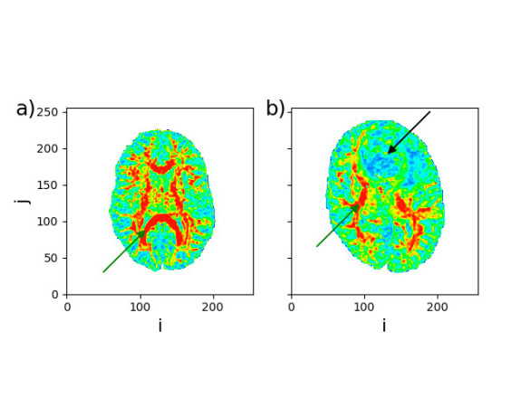
Figure 1: MRI slices of a) a healthy brain (slice 19 out of 44, control H(1)) and b) a tumorous brain (slice 19 out of 43, patient P(1)). The color grading represents the fractional anisotropy values, i.e. local density of neuron axons. The green arrows point to the corpus callosum areas and the black arrow in (b) to the tumorous area.

In the following sections we mostly present numerical results from control subject H(1) and patient P(1), but similar results and conclusion are drawn from the other two subjects.

III The Models

To explore the validity of our method and the consistency of our results across different neuronal models we use here two paradigmatic models for the numerical integration of the potentials: the FitzHugh-Nagumo (Sec. III.1) and the Leaky Integrate-and-Fire (Sec. III.2) models. The dynamics of the two models and and their implementation in neuronal networks are first described and at the end, in Sec. III.3, the construction of the coupling matrix is presented, making use of the MRI-DTI data of the healthy and destructed brain topology.

III.1 The FitzHugh-Nagumo Model

The single FHN oscillator model was introduced in early 1960s and consists of two coupled, nonlinear equations, one describing the evolution of a fast activator potential variable $\displaystyle u(t)$ and the other a slower inhibitor variable $\displaystyle v(t)$ FitzHugh (1961); Nagumo, Arimoto, and Yoshizawa (1962):

$$\displaystyle\epsilon\frac{du}{dt} \displaystyle=u-\frac{u^{3}}{3}-v$$ (1a)

$$\displaystyle\frac{dv}{dt} \displaystyle=u+{\rm a}.$$ (1b)

In Eq. (1a), $\displaystyle\epsilon$ is a parameter which accounts for the time-scale difference and is fixed in this study at $\displaystyle\epsilon=0.05$. The parameter $\displaystyle\rm a$ defines the dynamical behavior of Eqs. (1). For $\displaystyle|{\rm a}|<1$ the system contains an unstable fixed point, while for $\displaystyle|\rm a|>1$ the fixed point becomes stable. In the region $\displaystyle|\rm a|<1$ the unstable fixed point gives rise to a limit cycle through a Hopf bifurcation scenario. Throughout this study the parameter $\displaystyle\rm a$ is set to $\displaystyle\rm a=0.5$, in order to assure the presence of the limit cycle. For these parameter values the period of the uncoupled FHN oscillator is 2.7 time units.

FHN oscillators will be used in this study to model the dynamics in each voxel recorded by the MRI-DTI imaging technique. All voxels which have non-zero density of neuron axons (non-white color in Fig. 1) are equipped with an FHN oscillator.

The communication between the oscillators is dictated by the connectivity matrix $\displaystyle\sigma_{ijk:lmn}$ which connects the oscillator residing in voxel with 3D coordinates $\displaystyle(i,j,k)$ with the one in voxel $\displaystyle(l,m,n)$ (see details in Sec. III.3).

Omelchenko et al., in Ref. Omelchenko et al. (2013), have shown analytically and numerically that the coupled FHN model produces nontrivial partial synchronization patterns when activator-inhibitor cross coupling terms are involved. An account of different functional interactions is given in Pereda (2014), while a variety of activator-inhibitor coupling schemes used in a biological framework is reviewed in Ref. Kiskowski et al. (2004). Here, we use a coupling matrix with strong cross-coupling terms as proposed in Refs.  Omelchenko et al. (2013); Omel’chenko (2018). The coupled FHN dynamics is given by the following scheme:

$$\displaystyle\epsilon\frac{du_{ijk}}{dt} \displaystyle=u_{ijk}-\frac{u_{ijk}^{3}}{3}-v_{ijk}-\sum_{(l,m,n)}\sigma_{lmn:ijk}\left[b_{uu}(u_{lmn}-u_{ijk})+b_{uv}(v_{lmn}-v_{ijk})\right]$$ (2a)

$$\displaystyle\frac{dv_{ijk}}{dt} \displaystyle=u_{ijk}+{\rm a}-\sum_{(l,m,n)}\sigma_{lmn:ijk}\left[b_{vu}(u_{lmn}-u_{ijk})+b_{vv}(v_{lmn}-v_{ijl})\right]$$ (2b)

All FHN oscillators have the same parameters $\displaystyle\rm a$ and $\displaystyle\epsilon$ and the sums run over all voxels. The form of the coupling matrix restricts the interaction between distant voxels and accounts for the boundary conditions, as will be discussed in Sec. III.3. A rotational matrix, $\displaystyle B$, is a simple way to parameterize the possibility of diagonal coupling $\displaystyle(b_{uu},b_{vv})$ and activator-inhibitor cross coupling $\displaystyle(b_{uv},b_{vu})$ by a single parameter $\displaystyle\varphi$, which is close to $\displaystyle\pi/2$ if cross-coupling is dominant Omelchenko et al. (2013). This coupling phase $\displaystyle\varphi$ is similar to the phase-lag parameter $\displaystyle\alpha$ of the paradigmatic Kuramoto phase oscillator model, which is widely used to generically describe coupled oscillator networks. The coupling phase is necessary for the modeling of nontrivial partial synchronization patterns, as has been shown for the Kuramoto model Omel’chenko, Wolfrum, and Maistrenko (2010) and for the FHN model Omelchenko et al. (2013). This rotational matrix $\displaystyle B$ was later used in Refs. Omelchenko et al. (2015); Schmidt et al. (2017); Ramlow et al. (2019); Mikhaylenko et al. (2019) and has the form:

$$B=\begin{pmatrix}b_{uu}&b_{uv}\\ b_{vu}&b_{vv}\end{pmatrix}=\begin{pmatrix}\cos{\varphi}&\sin{\varphi}\\ -\sin{\varphi}&\cos{\varphi}\end{pmatrix}.$$ (3)

In the present study the value of the coupling phase $\displaystyle\varphi=\pi/2-0.1$ is used. $\displaystyle\varphi$-values in a narrow band around $\displaystyle\varphi=\pi/2$ are known to lead to coexistence of coherent and incoherent domains in networks consisting of FHN oscillators Omelchenko et al. (2013).

III.2 The Leaky Integrate-and-Fire model

The LIF model, introduced in 1907 by Louis Lapicque Brunel and van Rossum (1999); Abott (2007), describes the potential activity of isolated neurons via a single dynamical variable $\displaystyle u$. The evolution equation of the variable $\displaystyle u$ comprises two stages, an integration stage, Eq. (4a), and an abrupt resetting stage, Eq. (4b) :

$$\displaystyle\frac{du}{dt}=\mu-u,$$ (4a)

$$\displaystyle\lim_{\varepsilon\to 0}u(t+\varepsilon)\to u_{\text{rest}},\>\>\>\text{when}\>\>u\geq u_{\text{th}}.$$ (4b)

The second of the two equations represents the resetting condition: If the membrane potential reaches a threshold $\displaystyle u_{\text{th}}<\mu$, it is reset to a resting potential $\displaystyle u_{\text{rest}}$. Without loss of generality, we use the following parameter set: the parameter $\displaystyle\mu$ which represent the maximum achievable potential is set to $\displaystyle\mu=1$, the threshold potential is set to $\displaystyle u_{\text{th}}=0.98$ and the reset or resting potential is set to $\displaystyle u_{\text{rest}}=0$. For these parameter values the period of the uncoupled LIF oscillator is $\displaystyle T_{s}=3.91$ time units.

During the integration stage, Eq. (4a) behaves linearly and it can be solved analytically to obtain the neuron potential as: $\displaystyle u(t)=\mu-\left(\mu-u_{0}\right)e^{-t}$, with the initial condition $\displaystyle u(0)=u_{0}$. This behavior is repeated after each resetting, while the period $\displaystyle T_{s}$ of the single (uncoupled) LIF oscillator depends on $\displaystyle u_{\text{rest}}$ and $\displaystyle u_{\text{th}}$, as $\displaystyle T_{s}=\ln\left[\left(\mu-u_{\text{rest}}\right)/\left(\mu-u_{\text{th}}\right)\right]$. Although the neurons are known to spend a refractory period after the resetting stage, in this study the refractory period will be set to 0.

The coupling in the case of the LIF model follows the same scenario as in the FHN model described in the previous section. The coupling is even simpler, since there is only one variable and thus a rotational matrix is not needed. Here, all voxels recorded in the MRI image which have non-zero density of neuron axons (non- white color in Fig. 1) are equipped with a LIF oscillator. The connectivity matrix between the oscillators is the same in the LIF and FHN models, $\displaystyle\sigma_{ijk:lmn}$, see Sec. III.3. The LIF coupled network dynamics reads:

$$\displaystyle\frac{du_{ijk}}{dt}=\mu-u_{ijk}-\sum_{(l,m,n)}\sigma_{lmn:ijk}\left[u_{lmn}-u_{ijk}\right],$$ (5a)

$$\displaystyle\lim_{\varepsilon\to 0}u_{ijk}(t+\varepsilon)\to u_{\text{rest}},\>\>\>\text{when}\>\>u_{ijk}\geq u_{\text{th}}.$$ (5b)

All oscillators of the network have the same parameters, $\displaystyle u_{\text{th}}$, $\displaystyle u_{\text{rest}}$, $\displaystyle\mu$, while each one of them is reset independently, when reaching the threshold potential, $\displaystyle u_{\text{th}}$, common to all oscillators. In the present study we use values $\displaystyle u_{\text{rest}}<u_{\text{th}}<\mu$ and, therefore, the oscillators remain supra-threshold; their potentials take values between $\displaystyle u_{\text{rest}}$ and $\displaystyle u_{\text{th}}$. Regarding initial conditions, all oscillators start from $\displaystyle u_{ijk}(t=0)$ values randomly distributed between $\displaystyle 0\leq u_{ijk}(t=0)<u_{\text{th}}$.

We stress that in the present study both models, LIF and FHN, operate in the parameter regions which supports regular, periodic, self-sustained oscillations in the absence of any coupling.

III.3 Connectivity

Two types of connectivity matrices are used: $\displaystyle\sigma^{H}$ is the generic name for matrices extracted from the MRI-DTI data of healthy controls and $\displaystyle\sigma^{P}$ corresponds to the matrices extracted from the data of patients.

Generally, the MRI-DTI data (fractional anisotropy values) give the local density $\displaystyle I(i,j,k)$ of neuron axons present in the voxel centered around the coordinates $\displaystyle(i,j,k)$. The element of the connectivity matrix ($\displaystyle\sigma^{H}$ for the healthy subjects and $\displaystyle\sigma^{P}$ for the patients) which links voxels $\displaystyle(l,m,n)$ and $\displaystyle(i,j,k)$, is computed as:

$$\displaystyle\sigma_{ijk:lmn}=\begin{cases}\dfrac{h}{N_{R}}\dfrac{I(i,j,k)\>\>I(l,m,n)}{\displaystyle{\sum_{\rm all\>voxel-pairs}I(p1,p2,p3)\>\>I(q1,q2,q3)}},&\text{where}\>\>\>(i-l)^{2}\leq R^{2},\>\>\>(j-m)^{2}\leq R^{2}\>\>\>\text{and}\>\>\>n=k\pm 1\\ 0,&\text{otherwise}.\end{cases}$$ (6)

The product in the numerator of formula (6) ensures that only if there is nonzero white matter intensity in both $\displaystyle(l,m,n)$ and $\displaystyle(i,j,k)$ voxels interconnection between the voxels takes place. The sum over all pairs $\displaystyle(p1,p2,p3)$ and $\displaystyle(q1,q2,q3)$ in the denominator is set for normalization purposes. The network exchanges are limited to distances less than a given $\displaystyle R$ in the x-y plane (slice) and each slice is linked only to the layers above and below it, $\displaystyle n=k+1,\>k-1$. In this way the brain is considered as a multilayer network Majhi, Perc, and Ghosh (2016); Schöll, Zakharova, and Andrzejak (2019) consisting of $\displaystyle n_{s}$ layers, where each node $\displaystyle(i,j,k)$ interacts with nodes $\displaystyle(i-R,j,k)$, $\displaystyle(i-R+1,j,k)$ … $\displaystyle(i+R,j,k)$ and $\displaystyle(i,j-R,k)$, $\displaystyle(i,j-R+1,k)$ … $\displaystyle(i,j+R,k)$ in the same slice, and with nodes $\displaystyle(i,j,k+1)$ and $\displaystyle(i,j,k-1)$ in the perpendicular direction. The total number of links of each unit, denoted by $\displaystyle N_{R}$, is at most $\displaystyle(2R+1)^{2}+1$, i.e., $\displaystyle(2R+1)^{2}-1$ in its layer, plus 2 nodes above and below, in the axial direction. The factor $\displaystyle N_{R}$ counts the number of interacting neighbors and is set in the denominator for normalization purposes and ensures proportional contribution of each node in the sum. Note that the nodes which belong to the borders of the structure have less than $\displaystyle(2R+1)^{2}+1$ neighbors. For these nodes the $\displaystyle\sigma_{ijk:lmn}$ elements are divided by the number of existing neighbors. Overall, the coupling terms are multiplied (leveled) by a factor $\displaystyle h$ to modulate the intensity of the interactions.

We recall from Sec. II that the connectivity matrices used in this study are 3D with planes of size $\displaystyle 256\times 256$ and are composed by $\displaystyle 40\leq n_{s}\leq 44$ such planes. The coupling range $\displaystyle R=25$ is used, which is an intermediate coupling between local interactions $\displaystyle R=1$ and all-to-all coupling. This intermediate $\displaystyle R$-value accounts both for nearest neighbor interactions which are attributed to electrical exchanges and long distance coupling which is mediated by neurotransmitters. Intermediate coupling ranges between global (all-to-all) and nearest-neighbor connectivities are observed in many natural systems. Previous studies Omelchenko et al. (2013, 2015) have shown that there exists a quite wide intermediate range where the partially synchronized patterns, chimera states, can be observed. Moreover, these patterns are robust to the inhomogeneity of the network nodes or slight changes in the topology. We select an exemplary value for $\displaystyle R$ in our numerical simulations, but other values of $\displaystyle R$ in the range $\displaystyle 10\leq R\leq 60$ give qualitatively consistent results.

To avoid misunderstanding between structural and functional connectivity matrices, we stress here that the matrices extracted using Eq. 6, are structural, weighted connectivity matrices which are directly recorded by MRI scanners using the MRI-DTI technique. These matrices are not directly related with the functional connectivity matrices used in the literature. For the formation of the functional connectivity matrices the brain is lumped in 60-90 functional cortical regions and the exchanges between these regions are established using mostly EEG techniques and more recently MRI techniques Hagmann, Cammoun, and et al. (2008); Castro et al. (2020); Carboni, Rubega, and et al. (2019); Griffa, Baumann, and et al. (2019). Instead, in this work the spatial arrangement of the voxels is taken into account as directly represented by the MRI images. Nevertheless, the use of a dynamic model (FHN or LIF) in the network simulations allows us to extract functional synchronization patterns.

Following the above rules the full spatial connectivity matrices are constructed for the healthy and patient subjects and these matrices are used in Eqs. (2) and (5) for the integration of the potentials.

IV Results

In this section we present the results of numerical integration of the FHN equations and the LIF equations where each voxel is considered as an oscillatory unit with connectivity matrices obtained as discussed in the previous section, III.3. Firstly, the synchronization properties of the healthy control subject will be presented (section IV.1) followed by the patient results (section IV.2). To test the validity of the results, the same MRI-DTI data of the control subject and the patient will be used in sections IV.3 and IV.4, respectively, but the LIF dynamics will be used for the numerical integration. Although the dynamical schemes employed are entirely different, we demonstrate that the main qualitative synchronization patterns persist and the pacemaker effect which differentiates the control subjects from the patients is evident using both dynamical systems.

As working parameters the following sets were used: For the FHN system $\displaystyle\epsilon=0.05$, $\displaystyle\rm a=0.5$, $\displaystyle\varphi=\pi-0.1$, $\displaystyle h=0.1$; for the LIF model, $\displaystyle\mu=1.0$, $\displaystyle u_{\rm rest}=0.0$, $\displaystyle u_{\rm th}=0.98$, $\displaystyle h=0.6$ and the coupling parameter is $\displaystyle R=25$ in all cases. In the simulations both the Runge-Kutta 4th order method with integration step $\displaystyle 10^{-2}$ and the Euler method with integration step $\displaystyle 10^{-3}$ and $\displaystyle 10^{-4}$ were used.

IV.1 FHN Results on Healthy Brain Structure

FHN oscillators were placed on all voxels containing neuron axons. As an example, in plane (slice) 19 shown in Fig. 1a identical FHN units were placed on all non-white cells and similarly for all other planes above and below this. The FHN units were coupled nonlocally along the x-y plane and locally along the z-axis constituting a multilayer network composed of $\displaystyle n_{s}=44$ layers along the z-axis, as described in Sec. III.3 and Eq. (6). The connectivity matrix, $\displaystyle\sigma^{H}$, used here was extracted from the data of the healthy subject H(1) following the discussions in sections II and  III.3. Numerical integration of the corresponding Eqs. (2) and (3) was carried out for 2000 time units starting from random initial conditions (potentials).

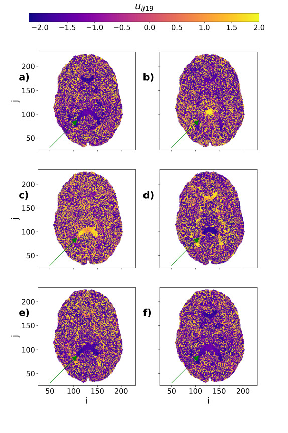
Figure 2: Color-coded typical potential profiles (snapshots) of slice 19 of healthy control H(1) using FHN dynamics. The profiles are recorded at a) 847.0, b) 847.8, c) 848.3, d) 849.0, e) 849.4 and f) 849.8 time units within one complete period. The green arrows point to the cc areas. Simulations start from random initial potentials. Other parameters are: $\displaystyle h=0.1$, $\displaystyle\varphi=\pi-0.1$, $\displaystyle\epsilon=0.05$, $\displaystyle\rm a=0.5$ and $\displaystyle R=25$.

After a transient period the network stabilizes in a state where the cc ribbon areas, set $\displaystyle A(H)_{\rm FHN}$, constitute the coherent parts, while the rest of the brain, the complement set $\displaystyle\overline{A(H)_{\rm FHN}}$ is incoherent. Representative color-coded potential results on slice 19 are presented in Fig. 2. These are typical steady state snapshots showing the different phases of the slice. The green arrows point to the cc areas. The six representative snapshots are all recorded within an interval of 3 time units, which is the maximum period observed in the system. In particular: panel a) is characterized by low, common potential values in all cc areas and by mixed state of the complement set; in panel b) the potential in the middle of the lowest cc area starts increasing (becoming yellow) while the complement set keeps in the incoherent state; in panel c) the yellow color (high potential values) invades the lower cc area, while the higher cc area also increases its potentials and becomes hidden within the incoherent set; in panel d) the potentials in the lower cc area start increasing (becoming dark blue) from the center, while the upper cc area becomes again visible having simultaneously acquired the high potential values (yellow colors); in panel e) the low potentials (dark blue colors) start invading the lower cc area while the potentials in the upper cc area take intermediate values (orange colors) and in panel f) all cc areas acquire the lowest (dark blue) potential values. The f) state is equivalent to state a) and are considered as the starting point of a new period. Note that in regards to the cc areas, panels b) and d) are in opposite phases of each other.

From the results in Fig. 2 we note that while in the cc areas the potentials are identical or follow closely their neighboring values, the complement sets are always in the incoherent state. This behavior can be considered as a “chimera-like” state. (Note that the cc areas correspond to brain regions of high density, where the connectivity between the two hemispheres, left $\displaystyle\leftrightarrow$ right, dominates, see Fig. 1a.) We recall here that the term “chimera state” is reserved to networks where synchronous and asynchronous regions coexist under the condition that all nodes are identical and identically linked. In the present case, all oscillators are identical but the linking is not homogeneous since it is recorded from the MRI-DTI data of a real healthy brain. For this reason, as explained in the Introduction, the term “chimera-like state” is used.

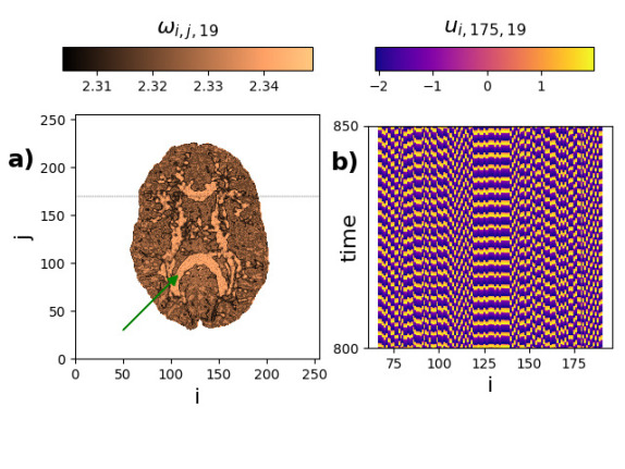
Figure 3: a) Mean phase velocity profile of slice 19 of healthy subject H(1) using FHN dynamics. b) Spacetime plot corresponding to the cut for $\displaystyle j=175$ indicated in (a) with the grey line. The green arrow points to the cc area. The average in (a) was taken over 2000 time units. Other parameters as in Fig. 2.

The chimeric nature of the coupled system can be further verified using the mean phase velocity profile. The mean phase velocity $\displaystyle\omega_{ijk}$ accounts for the number of cycles $\displaystyle c_{ijk}$ that oscillator at position $\displaystyle(i,j,k)$ has performed during a certain time interval $\displaystyle\Delta T$, and is defined as:

$$\displaystyle\omega_{ijk}=2\pi\frac{c_{ijk}}{\Delta T}=2\pi f_{ijk}\>\>,$$ (7)

where $\displaystyle f_{ijk}$ is the frequency of the oscillator. Because the definitions of frequency and mean phase velocity differ by just a factor $\displaystyle 2\pi$, in the following the two expressions are used interchangeably.

The cc ribbon sets $\displaystyle A(H)_{\rm FHN}$ of slice 19 demonstrate common mean phase velocity and they clearly correspond to the cc ribbon sets $\displaystyle A(H)$ of the MRI-DTI data, compare Figs. 1a and  3a (the green arrows point always to the cc areas). The mean phase velocity over the ribbon set is constant and is consistently higher than in the rest of the structure. Returning to Fig. 2, on the lower cc ribbon area we can discern color-grading which corresponds to traveling waves in the corpus callosum. These are more evident in the videos included in the Supplementary Material (Multimedia view). The traveling waves disappear in the complement set $\displaystyle\overline{A(H)_{\rm FHN}}$ and they are held responsible for the higher mean phase velocities observed in the cc areas.

To elucidate further the nature of oscillations in the healthy brain, in Fig. 3b we present the spacetime plot of the potential along a line crossing slice 19 at position $\displaystyle j=175$, see grey horizontal line in Fig. 3a. This line was chosen because on the one hand it crosses both $\displaystyle A(H)_{\rm FHN}$ and $\displaystyle\overline{A(H)_{\rm FHN}}$ sets in the healthy brain and, on the other hand, it crosses at the same level the tumorous regions in the patient P(1) brain (see Sec. IV.2 and Fig. 5, later on). In Fig. 3b, it is possible to see that the synchronous cc regions coexist with the asynchronous complement $\displaystyle\overline{A(H)_{\rm FHN}}$, forming the chimera-like state.

IV.2 FHN Results on Anomalous Brain Structure

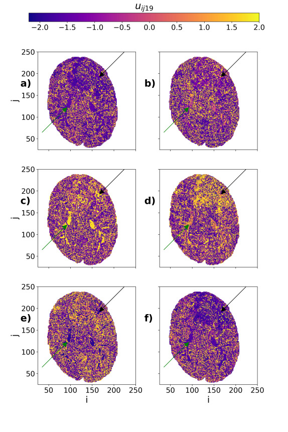
Figure 4: Color-coded typical potential profiles of slice 19 of patient P(1) with destructed brain structure using FHN dynamics. The profiles are recorded at a) 382.9, b) 383.5, c) 383.9, d) 384.4, e) 384.7 and f) 385.4 time units. The green arrows point to cc areas and black arrows point to the tumorous area. Simulations start from random initial potentials. Other parameters as in Fig. 2.

Exactly the same numerical simulation process was applied here, as in the previous section IV.1, the only difference being that now the connectivity matrix, $\displaystyle\sigma^{P}$, extracted from the patient P(1) was used. Namely, identical FHN oscillators were placed on all voxels and these where coupled nonlocally along the x-y plane and locally along the z-axis. Numerical integration of Eqs. (2) using the connectivity matrix $\displaystyle\sigma^{P}$ were carried out for 2000 time units starting from random initial potentials. The color-coded potential results on slice 19 are presented in Fig. 4 at six different instances within the maximum period of oscillations. At all instances, the cc structure (see green arrows) is presented damaged, as also shown in the MRI-DTI data (Fig. 1b).

A new observation is the “pacemaker effect” which is more clearly visible in the supplementary video (Multimedia view) and also appears in the simulations using the LIF model in section  IV.4. Namely, potential waves are initiated in the tumorous region (see black arrows in Fig. 4), they propagate through the white matter and they disappear at the borders of the brain structure before a new potential wave restarts at the tumorous region. More precisely, in panel 4a) the regions around the tumorous areas demonstrate low (dark blue) potentials similar to the destructed cc areas; in panel b) the potentials in the tumorous area increase toward orange-yellow values and so do the cc areas; in panel c) the tumorous areas acquire maximum potential values; in d) the maximum potential values propagate away from the tumor in the cc-complement set while the cc set has intermediate (orange colored) values; in e) the potentials in the tumorous regions start decreasing toward dark blue values and in f) the dark blue values propagate covering the tumorous region, while the cc regions also acquire the lowest potential values. Panel f) corresponds to panel a) which was considered as the starting stage of a period. The gradual propagation of the yellow color from the tumorous areas to the rest of the brain (sequence of panels b) $\displaystyle\to$ c) $\displaystyle\to$ d) ) illustrates the pacemaker effect which is centered in the lesion and can be used potentially to identify the position of the tumor.

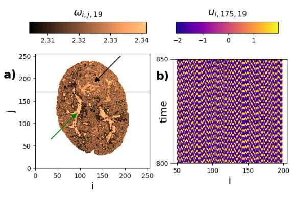
Figure 5: a) Mean phase velocity profile of slice 19 of the subject P(1) with destructed brain structure using FHN dynamics. b) Spacetime plot corresponding to the cut for $\displaystyle j=175$ indicated in (a) with the grey line which crosses the lesion. The average in (a) was taken over 2000 time units. The green arrow points to cc areas and the black arrow to the lesion area. Other parameters as in Fig. 2.

The associated mean phase velocity profile in Fig. 5a indicates clearly the positions of the destructed ribbon structure (see green arrow), where high $\displaystyle\omega$ values are observed. In the same image the tumorous area is shown, marked by the black arrow, where also relatively high mean phase velocities are recorded. Comparing Figs. 3a and 5a, it is evident that high $\displaystyle\omega$’s dominate in the position where the potential waves are initiated in the lesion area.

Similarly to the healthy case, Fig. 3b, in Fig. 5b the spacetime plot of the potential along a line crossing slice 19 at position $\displaystyle j=175$ is presented (see grey horizontal line in Fig. 5a). This line now crosses the tumorous regions. In Fig. 5b, it is not possible to discern any synchronous region. The tumor has destructed the tissue structure and the chimera-like profile observed in the healthy brain, Fig. 3b, is no longer manifested. This difference can be used as an indicator of malignancy and can be critical in cases where the tumor is small, not visible by eye, but it can destroy the chimera-like patterns and induce brain waves through the pacemaker effect.

Although the results presented in the above two sections depict layer 19 for the healthy and the patient subjects, qualitatively similar results and conclusions are drawn from all other layers in the network. In the next two sections, the FHN dynamics is replaced by the LIF model dynamics and it is shown that the pacemaker effect is robust across models (is not model dependent) since it comes as a result of the brain structure anomalies.

IV.3 LIF Results on Healthy Brain Structure

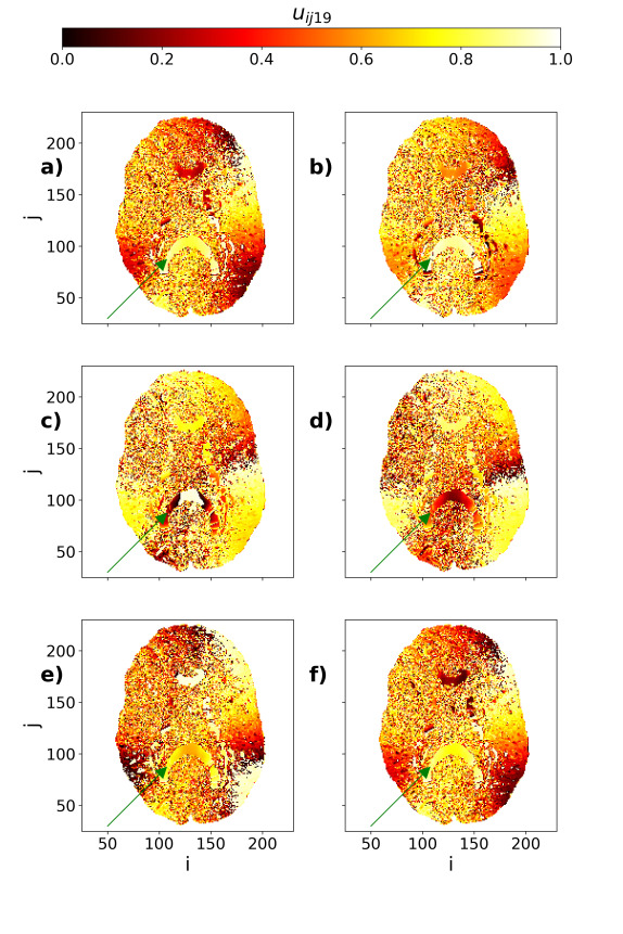
Figure 6: Color-coded potential profile of slice 19 of healthy control H(1) using LIF dynamics. The profiles are recorded at a) 846.7, b) 847.2, c) 847.8, d) 848.2, e) 849.0 and f) 849.4 time units (for comparison with healthy brain network dynamics in section IV.1 ). Simulations start from random initial potentials. Other parameters are: $\displaystyle h=0.6$, $\displaystyle\mu=1.0$, $\displaystyle u_{\rm rest}=0.0$ and $\displaystyle u_{\rm th}=0.98$. Green arrows as in Fig. 2.

In this section, the LIF scheme, Eq. (5), is employed to simulate the dynamics on all nodes of the healthy subject H(1). The connectivity matrix used is $\displaystyle\sigma^{H}$, the same one which was used in section IV.1. All oscillators start from random initial potentials in the range [0,$\displaystyle u_{\rm th}$]. Figure  6 depicts six color-coded potential profiles of representative slice 19, centrally located on the vertical axis of the head. These typical profiles represent the various phases that the cc and complement domains undergo within one period of LIF oscillations.

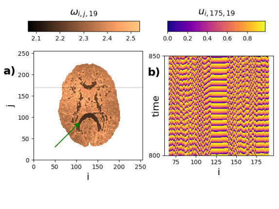
Figure 7: a) Mean phase velocity profile of slice 19 of healthy subject H(1) using LIF dynamics. b) b) Spacetime plot corresponding to the cut for $\displaystyle j=175$ indicated in (a) with the grey line. The average in (a) was taken over 2000 time units. Green arrow as in Fig. 3. Other parameters as in Fig. 6.

Clearly, two different regions can be identified in all six panels: a) A set $\displaystyle A(H)_{\rm LIF}$ consisting of the isolated cc segments which present phase coherence (green arrows in Fig. 6) and b) the complement $\displaystyle\overline{A(H)_{\rm LIF}}$ of this set where the phases are incoherent. The sets $\displaystyle A(H)_{\rm LIF}$ and $\displaystyle\overline{A(H)_{\rm LIF}}$ overlap with the corresponding sets $\displaystyle A(H)$ and $\displaystyle\overline{A(H)}$ of the MRI-DTI data of the healthy subject H(1). A simple comparison between LIF and FHN numerical results indicates that the sets $\displaystyle A(H)_{\rm LIF}$ and $\displaystyle\overline{A(H)_{\rm LIF}}$ (see Fig. 6) present the same characteristics with the corresponding sets $\displaystyle A(H)_{\rm FHN}$ and $\displaystyle\overline{A(H)_{\rm FHN}}$ resulting from FHN simulations (see Fig. 2).

The panels in Fig. 6 demonstrate the LIF activity within one period of oscillations. For clarity we present here the evolution within the cc regions which in the LIF model keep a constant phase difference. In panel a) the lower cc region is characterized by high (yellow) potential values while the top cc region has intermediate (red) values; in panel b) the potentials increase in the lower cc region becoming almost white (value $\displaystyle u_{ijk}\sim 1.0$), with a similar increase in the top cc area toward orange color; in panel c) the center of the lower cc region is still in the range of higher ($\displaystyle u_{ijk}\sim 1.0$) values while its border voxels have dropped to zero (black and dark red color) due to the resetting condition, Eq. 5b, and the top cc region potentials increase toward yellow values; in panel d) the dark and red regions (low potentials) have now invaded the lower cc area, while in the upper one the potentials increase further; in panel e) the potentials in the lower cc area increase toward orange-yellow values while in the top cc area the potentials have reached their maximum values ($\displaystyle u_{ijk}\sim 1.0$) and in panel f) the lower cc area potentials increase further (yellow colors) while in the upper cc area resetting occurs and the potential values drop to dark and red values. This last panel f) is similar to panel a) which is taken as the starting point of a new period. The related video provided in the Supplementary Material shows that a) the cc areas behave coherently demonstrating a consistent phase difference between the upper and lower regions and b) the activity in the complement is in the form of irregular potential waves which appear and disappear in the periphery of the brain (Multimedia view).

The mean phase velocity profile of the same plane demonstrates the coexistence of coherent and incoherent domains, see Fig. 7a. The cc ribbons of high white matter density, set $\displaystyle{A(H)_{\rm LIF}}$, appear here undestructed, their $\displaystyle\omega$-values present consistently lower values than the surrounding complement set and depict the same structure as set $\displaystyle A(H)$ of the MRI-DTI data, Fig. 1a.

Figure 7b depicts the spacetime plot of a linear cut along the slice 19, at position $\displaystyle j=175$, as designated in Fig. 7a with the grey line. At the position where this cut crosses the cc ribbons, $\displaystyle 120<i<135$, a coherent domain is noted in the spacetime plot. This finding, using the LIF dynamics, agrees with similar findings depicted in Fig. 3 and Sec. IV.1, where the FHN dynamics was employed. The fact that both FHN and LIF dynamics confirm the presence of chimera-like patterns in the healthy brain is an indication that this effect is model independent and is caused by the interplay between the complex connectivity and the nonlinear dynamics added in the network.

IV.4 LIF Results on Anomalous Brain Structure

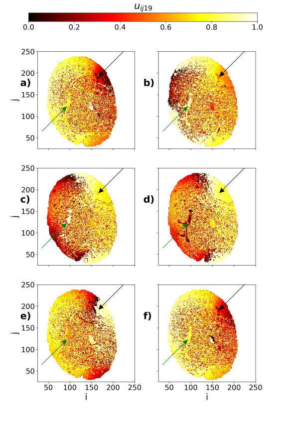
Figure 8: Color-coded potential profiles of slice 19 of subject P(1) with destructed brain structure using LIF dynamics. The six profiles are recorded at a) 350.7, b) 351.4, c) 351.9, d) 352.2, e) 352.9 and f) 353.6 time units. Simulations start from random initial potentials. Green and black arrows as in Fig. 4. Other parameters as in Fig. 6.

The numerical integration results on anomalous brain structure using the LIF dynamics are in qualitative agreement with the ones obtained using the FHN dynamics. To illustrate this, in Fig. 8 we present the representative phases characteristic of the potential profiles: in panel a) the tumorous region is in the lowest potential values (black and red colors) while the destructed cc area marked by the green arrow is characterized by higher (yellow) potentials; in panel b) the potentials in the tumorous region increase toward orange values while the cc area potentials increase further toward lighter yellow; in panel c) we observe further increase in the tumorous region toward yellow, while the cc area has reached maximum (white) potentials; in panel d) the tumorous region potentials increase toward lighter yellow while the cc pointed area potentials were reset to low values (dark, red); in panel e) the tumorous region develops maximum (white) potentials while the $\displaystyle u$-values increase in the cc pointed ribbon toward medium (orange) values and in panel f) the potentials are reset in the tumorous region (dark, red colors) and the $\displaystyle u$-values in the cc region increase to high (yellow) values. Note that panels a) and f) correspond to equivalent states and are selected as the starting points of a new period. Here the remaining disjoint pieces of the cc areas present a phase shift in their potential values. For example, in panel a) the right cc area is white-colored, higher than the left one (yellow colored). In panel b) the right cc area was reset to low values while the left one increases further toward maximum potentials, and so on.

The six panels of Fig. 8 are indicative of the pacemaker effect induced by the tumorous region which can be also seen in the following way: In panel a) a yellow colored region appears in the left-top periphery of the brain. In panel b) it gives rise, after resetting, to black and red regions. In panel c) the black-red region splits in two which propagate peripherally toward the tumorous regions. In panel d) the black and red regions (low potentials) propagate further toward the tumor, while behind them, to the left, the yellow region restarts developing. In panel e) the red regions approach further the tumorous area while behind them the yellow region extends covering the entire left semiplane. In panel f) the red areas have covered/invaded the tumorous region returning to a state similar to a). The effect is more clear in the corresponding video provided in the Supplementary Material (Multimedia view). After a transient period of about 200 time units, the waves created in the periphery of the brain collide in the tumorous region and disappear there. In this case, the pacemaker acts as an absorber of the potential waves propagating circularly in the brain periphery. This behavior is similar to the pacemaker effect that was also observed in the FHN model with the difference that here the pacemaker acts as an absorber, or a pacemaker with negative propagation.

The cc ribbon structure, set $\displaystyle A(P)_{\rm LIF}$ of high white matter density is also destructed in the LIF simulations, in agreement with the MRI-DTI data (Fig. 1b) and the FHN results (Fig. 4). The region where the potential waves collapse is identified as the blue region in Fig. 1b, where the lesion is located.

The corresponding mean phase velocity profile results, Fig. 9a, conform with the above discussion. The tumorous area indicated by the black arrow shows lower mean phase velocity than the center of the brain where the structure is less affected by the pathology. Figure 9b depicts the spacetime plot of a linear cut along the slice 19 at position $\displaystyle j=175$ (designated in Fig. 9a with the grey line), which crosses the tumorous region. Contrary to the case of healthy brain, Fig. 7b, the spacetime plot here does not contain a coherent domain, due to the destruction of the cc ribbon areas. Similar behavior was also noted earlier, in Fig. 5 and Sec. IV.2, where the FHN dynamics was used.

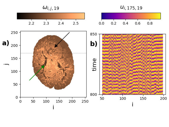
Figure 9: a) Mean phase velocity profile of slice 19 of subject P(1) with destructed brain structure using LIF dynamics. b) Spacetime plot corresponding to the cut for $\displaystyle j=175$ indicated in (a) with the grey line which crosses the tumorous region. The average in (a) was taken over 2000 time units. Green and black arrows as in Fig. 5. Other parameters as in Fig. 6.

The qualitative agreement in the pacemaker effect produced in the patient using both LIF and FHN dynamics comes as a result of the destruction of the brain structure and is not an artefact of the dynamics, since it appears independently in the two models when the tumorous region is introduced through the connectivity matrix. The anomaly in the present structure has a relatively large extension, as it was the case for this particular patient. It would be interesting to explore if similar pacemaker effects will be produced when smaller tumors are considered.

Overall, both FHN and LIF dynamical schemes confirm the presence of chimera-like patterns in the healthy brain while incoherent dynamics and pacemaker effects are observed in the destructed, tumorous brains. These phenomena seem to be generic and not model dependent or artefacts of a particular model.

V Spectral Analysis of Healthy and Anomalous Dynamics

In this section a first attempt is made to test whether the presence of the tumor affects the Fourier spectra of the neuronal oscillations locally, in the lesion areas. For this reason, we run long simulations for over 300 periods ($\displaystyle\sim$ 1000 time units) after disregarding the initial transient time and record every integration step for higher accuracy. Four sets of simulations were analyzed for each healthy and patient subjects using the FHN and the LIF models. In all cases, detailed recording over time were gathered from representative voxels.

In the following subsections typical voxels will be depicted in Figs. 10 and 11. For the healthy subject H(1), Fig. 1a, the presented voxels (i,j,k) are: (48,93,19) front left; (77,136,19) inside the cc area; (132,136,19) centrally located in the figure; (138,156,19) inside the cc area and (179,133,19) back front left area. For the patient P(1), Fig. 1b, the presented voxels are: (36,85,19) front left; (61,104,19) inside the tumorous area; (80,131,19) inside the tumorous area; (133,150,19) inside the cc area and (169,91,19) inside the cc area. Note that different voxels are used in each case, because the cc areas in the diseased subject were delocalized due to the presence of the tumor.

The time series recordings were Fourier transformed to detect the dominant frequencies and the results on subjects H(1) and P(1) of the FHN and LIF simulations are presented in Sec. V.1 and Sec. V.2, respectively. Additional results on the spectra of subjects H(2) and P(2) are included in the Supplementary Material (Multimedia view).

V.1 FHN Spectra

The Fourier spectra of the FHN dynamics in the neuron axons network of the healthy subject H(1) are presented in the top panel of Fig. 10. All nodes (voxels), independently of position, demonstrate the same frequency characteristics. Even the nodes residing in the cc areas demonstrate the same characteristics of the basic frequency component as the other nodes in the white matter, while small deviations are noted in the higher harmonics (not shown).

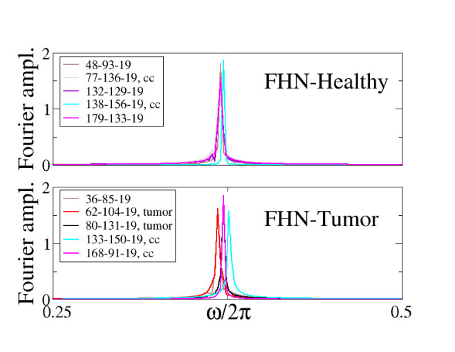
Figure 10: Fourier spectra of various voxels from FHN simulations. Top: Healthy subject H(1). Bottom: Patient P(1). The various colors correspond to the different voxels. In the subject with tumor the black and red lines correspond to voxels from the tumor area. The voxels denoted by cc are located in the corpus callosum areas. The spectra are computed over 300 cycles of the FHN dynamics. Other parameters as in Fig. 2.

A distinct difference is noted when there is a tumorous area as depicted in the lower panel of Fig. 10, which presents the Fourier spectra of the individual nodes when the connectivity matrix of the patient P(1) is used. In this case, the timeseries originating from different areas develop different collective frequencies, although in the simulations all elementary oscillators have identical natural frequencies. This difference in the spectra can be attributed to the inhomogeneity that the tumor induces in the brain and confirms the observation of the chimera-like states which was reported in the previous sections IV.2 and IV.4. The different contributions visible on the basic frequency (Fig. 10, lower panel) are accentuated on the first harmonic (not shown).

For the simulations in the present subsection, all parameters used are the same as in Fig. 2. Further studies in this direction, including the use of different FHN parameters, may enlarge the frequency difference in the tumorous brain and help to identify the affected regions even when their size is small.

V.2 LIF Spectra

The Fourier spectra when the LIF dynamics are used for the integration of the potential in the healthy and tumorous case are depicted in Fig. 11. The top (bottom) panel depicts the Fourier spectra of the healthy (patient) subject.

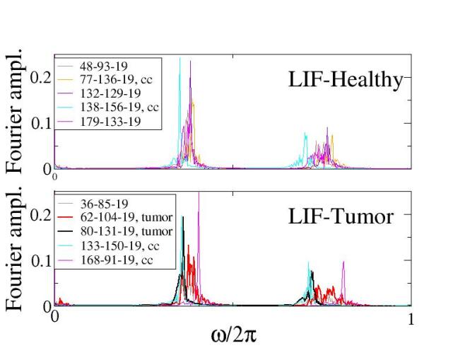
Figure 11: Fourier spectra of various voxels from LIF simulations. Top: Healthy subject H(1). Bottom: Patient P(1). Line colors and other notation as in Fig. 10. The spectra are computed over 300 cycles of the LIF dynamics. All parameters as in Fig. 4.

In both cases the spectra do not present a single frequency but a continuous band of frequencies, both around the basic frequency as well as its harmonics. For this reason it is not possible to clearly identify differences in the Fourier spectra between the voxels belonging to the tumorous regions and other non-tumorous areas. The results do not improve when longer time series (as long as $\displaystyle\sim$ 19000 time units) are considered.

These results give a first evidence that the FHN model dynamics may be more appropriate than the LIF model for distinguishing between healthy and tumorous areas in the brain when the Fourier spectra are used. Nevertheless, by adjusting parameters, such as $\displaystyle\alpha$ or $\displaystyle\phi$ in the FHN model, $\displaystyle u_{\rm th}$ in the LIF model and $\displaystyle h,\>R$ in the connectivity matrix we may achieve better discrimination levels.

VI Conclusions

Simulations inspired by the connectivity of the neuron axons network were conducted, based on MRI-DTI data from healthy and tumor suffering brains. Two neuronal models were used to simulate the dynamics in the individual voxels recorded from the MRI images, the FitzHugh-Nagumo and the Leaky Integrate-and-Fire models. In the healthy brain both models consistently differentiate between the corpus callosum regions, which are regions with high density of neuron axons, and the rest of the white matter. In tumorous brains, the destructed regions are clearly visible in the mean phase velocity diagrams of both models.

The numerical results demonstrate that the healthy brain presents chimera-like states where regions with high white matter concentrations in the direction connecting the two hemispheres act as the coherent domain, while the rest of the brain exhibits incoherent oscillations. To the contrary, in brains with destructed white matter structure traveling waves are produced initiated around the region where the tumor is located. These areas act as the pacemaker of the waves sweeping across the brain.

The present simulations, using specific parameter variables, give a first evidence of the pacemaker effect and the chimera-like states. It would be useful to scan further the parameter space of the FHN and LIF models to determine the parameter regions where these effects are accentuated. Further studies with more subjects and different sizes of tumors need to be assessed, to verify whether the pacemaker effect could be useful as indicator of brain tumorous states, with particular reference in cases of small, difficult to detect abnormalities.

In this study we have tested the FHN and LIF dynamics and have shown that both models give consistent results. In future studies other neuronal models can be implemented to evaluate the universality of these results across models. In particular, neuronal population dynamics models can be employed to represent the local dynamics on a single voxel and test whether this class of models leads to comparable conclusions.

In a different network approach, connectivity matrices might be constructed using nonlocal interactions over variable ranges. The properties of these matrices can be compared between control subjects and patients and these could also be examined as indicators/biomarkers of tumor. The form and statistics of the constructed (nonlocal) networks may also give some insights in the synchronization properties observed in the patients and the control subjects.

Apart for the cases of tumors, similar numerical studies might be conducted using neuron axons networks from MRI studies of brains suffering from Alzheimer, Parkinson or other disorders which affect the structure of the brain neurons and their connectivity networks.

Supplementary Material

See in the supplementary material the eight videos concerning the four subjects as follows a) FHN simulations of the healthy control brains (subjects H(1) and H(2)), b) FHN simulations of the patient (tumor) brains (subjects P(1) and P(2)), c) LIF simulations of the healthy control brains (subjects H(1) and H(2)), d) LIF simulations of the patient brains (subjects P(1) and P(2)).

Additional images are also uploaded as e) Fourier spectra of subjects H(2) and P(2) with FHN dynamics and f) Fourier spectra of subjects H(2) and P(2) with LIF dynamics.

Collections of 15 consecutive profiles are provided for each of the following cases: g) FHN simulations of subject H(1), h) FHN simulations of subject P(1), i) LIF simulations of subject H(1) and j) LIF simulations of subject P(1).

Data Availability Statement

The data that support the findings of this study are available from the corresponding author upon reasonable request.

References

- Gao and Jiang (2013) H. Gao and X. Jiang, “Progress on the diagnosis and evaluation of brain tumors,” Cancer Imaging 13, 466–481 (2013).
- Pratt and C.Stapelberg (2018) R. Pratt and N. J. C.Stapelberg, “Early warning biomarkers in major depressive disorder: a strategic approach to a testing question,” Biomarkers 23, 563–572 (2018).
- Galldiks et al. (2019) N. Galldiks, P. Lohmann, N. L. Albert, J. C. Tonn, and K.-J. Langen, “Current status of PET imaging in neuro-oncology,” Neuro-Oncology Advances 1, 1–11 (2019).
- Boccaletti et al. (2018) S. Boccaletti, A. N. Pisarchik, C. I. del Genio, and A. Amann, Synchronization: From coupled systems to complex networks (Cambridge University Press, Cambridge, 2018).
- Velazquez and Wennberg (2009) J. L. P. Velazquez and R. Wennberg, Coordinated Activityin the Brain, Springer Series in Computational Neuroscience, vol. 2 (Springer Science, 2009).
- Izhikevich (2007) E. M. Izhikevich, Dynamical Systems in Neuroscience: The Geometry of Excitability and Bursting (The MIT Press, Cambridge, 2007).
- Gerstner and Kistler (2002) W. Gerstner and W. M. Kistler, Spiking neuron models: Single neurons, populations, plasticity (Cambridge University Press, Cambridge, 2002).
- Kandel et al. (2013) E. R. Kandel, J. H. Schwartz, T. M. Jessell, S. A. Siegelbaum, and A. J. Hudspeth, Principles of Neural Science, 5th Edition (The McGraw-Hill Companies, Inc., New York, 2013).
- Andrzejak et al. (2016) R. G. Andrzejak, C. Rummel, F. Mormann, and K. Schindler, “All together now: Analogies between chimera state collapses and epileptic seizures,” Scientific Reports 6, 23000 (2016).
- Mormann et al. (2000) F. Mormann, K. Lehnertz, P. David, and C. E. Elger, “Mean phase coherence as a measure for phase synchronization and its application to the EEG of epilepsy patients,” Physica D 144, 358 (2000).
- Olmi et al. (2019) S. Olmi, S. Petkoski, M. Guye, F. Bartolomei, and V. Jirsa, “Controlling seizure propagation in large-scale brain networks,” PLoS Computational Biology 15, e1006805 (2019).
- Chouzouris et al. (2018) T. Chouzouris, I. Omelchenko, A. Zakharova, J. Hlinka, P. Jiruska, and E. Schöll, “Chimera states in brain networks: Empirical neural vs. modular fractal connectivity,” Chaos 28, 045112 (2018).
- Kuramoto and Battogtokh (2002) Y. Kuramoto and D. Battogtokh, “Coexistence of coherence and incoherence in nonlocally coupled phase oscillators,” Nonlinear Phenomena in Complex Systems 5, 380 (2002).
- Kuramoto (2002) Y. Kuramoto, “Reduction methods applied to nonlocally coupled oscillator systems,” in Nonlinear Dynamics and Chaos: Where do we go from here?, edited by S. J. Hogan, A. R. Champneys, A. R. Krauskopf, M. di Bernado, R. E. Wilson, H. M. Osinga, and M. E. Homer (CRC Press, 2002) pp. 209–227.
- Abrams and Strogatz (2004) D. M. Abrams and S. H. Strogatz, “Chimera states for coupled oscillators,” Physical Review Letters 93, 174102 (2004).
- Sakaguchi (2006) H. Sakaguchi, “Instability of synchronized motion in nonlocally coupled neural oscillators,” Physical Review E 73, 031907 (2006).
- Omelchenko et al. (2013) I. Omelchenko, O. E. Omel’chenko, P. Hövel, and E. Schöll, “When nonlocal coupling between oscillators becomes stronger: patched synchrony or multi-chimera states,” Physical Review Letters 110, 224101 (2013).
- Omelchenko et al. (2015) I. Omelchenko, A. Provata, J. Hizanidis, E. Schöll, and P. Hövel, “Robustness of chimera states for coupled FitzHugh-Nagumo oscillators,” Physical Review E 91, 022917 (2015).
- Schmidt et al. (2017) A. Schmidt, T. Kasimatis, J. Hizanidis, A. Provata, and P. Hövel, “Chimera patterns in two-dimensional networks of coupled neurons,” Physical Review E 95, 032224 (2017).
- Hizanidis et al. (2014) J. Hizanidis, V. Kanas, A. Bezerianos, and T. Bountis, “Chimera states in networks of nonlocally coupled Hindmarsh-Rose neuron models,” International Journal of Bifurcations and Chaos 24, 1450030 (2014).
- Ulonska et al. (2016) S. Ulonska, I. Omelchenko, A. Zakharova, and E. Schöll, “Chimera states in networks of Van der Pol oscillators with hierarchical connectivities,” Chaos 26, 094825 (2016).
- Olmi et al. (2015) S. Olmi, E. A. Martens, S. Thutupalli, and A. Torcini, “Intermittent chaotic chimeras for coupled rotators,” Physical Review E 92, 030901 (2015).
- Tsigkri-DeSmedt et al. (2017) N. D. Tsigkri-DeSmedt, J. Hizanidis, E. Schöll, P. Hövel, and A. Provata, “Chimeras in leaky integrate-and-fire neural networks: effects of reflecting connectivities,” The European Physical Journal B 90, 139 (2017).
- Tsigkri-DeSmedt et al. (2018) N. D. Tsigkri-DeSmedt, I. Koulierakis, G. Karakos, and A. Provata, “Synchronization patterns in lif neuron networks: Merging nonlocal and diagonal connectivity,” http://arxiv.org/abs/1807.11843 (2018).
- Santos et al. (2018) V. Santos, J. D. J. Szezech, A. M. Batista, K. C. Iarosz, M. S. Baptista, H. P. Ren, C. Grebogi, R. L. Viana, I. L. Caldas, , Y. L. Maistrenko, and J. Kurths, “Riddling: Chimera’s dilemma,” Chaos 28, 081105 (2018).
- Gjurchinovski, Schöll, and Zakharova (2017) A. Gjurchinovski, E. Schöll, and A. Zakharova, “Control of amplitude chimeras by time delay in dynamical networks,” Physical Review E 95, 042218 (2017).
- Zakharova et al. (2017) A. Zakharova, N. Semenova, V. S. Anishchenko, and E. Schöll, “Time-delayed feedback control of coherence resonance chimeras,” Chaos 27, 114320 (2017).
- Shepelev and Vadivasova (2019) I. Shepelev and T. Vadivasova, “Variety of spatio-temporal regimes in a 2d lattice of coupled bistable fitzhugh-nagumo oscillators. formation mechanisms of spiral and double-well chimeras,” Communications in Nonlinear Science and Numerical Simulation 79, 104925 (2019).
- Panaggio and Abrams (2015) M. J. Panaggio and D. Abrams, “Chimera states: Coexistence of coherence and incoherence in networks of coupled oscillators,” Nonlinearity 28, R67–R87 (2015).
- Schöll (2016) E. Schöll, “Synchronization patterns and chimera states in complex networks: Interplay of topology and dynamics,” European Physical Journal – Special Topics 225, 891–919 (2016).
- Yao and Zheng (2016) N. Yao and Z. Zheng, “Chimera states in spatiotemporal systems: Theory and applications,” International Journal of Modern Physics B 30, 1630002 (2016).
- Majhi et al. (2019) S. Majhi, B. K. Bera, D. Ghosh, and M. Perc, “Chimera states in neuronal networks: A review,” Physics of Life Reviews 28, 100–121 (2019).
- Omel’chenko (2018) O. E. Omel’chenko, “The mathematics behind chimera states,” Nonlinearity 31, R121 (2018).
- Zakharova (2020) A. Zakharova, Chimera Patterns in Networks: Interplay between Dynamics, Structure, Noise, and Delay (Understanding Complex Systems, Springer International Publishing, 2020).
- M.Hagerstrom et al. (2012) A. M.Hagerstrom, T. E. Murphy, R. Roy, P. Hövel, I. Omelchenko, and E. Schöll, “Experimental observation of chimeras in coupled-map lattices,” Nature Physics 8, 658 (2012).
- Tinsley, Nkomo, and Showalter (2012) M. R. Tinsley, S. Nkomo, and K. Showalter, “Chimera and phase-cluster states in populations of coupled chemical oscillators,” Nature Physics 8, 662 (2012).
- Wickramasinghe and Kiss (2013) M. Wickramasinghe and I. Z. Kiss, “Spatially organized dynamical states in chemical oscillator networks: Synchronization, dynamical differentiation, and chimera patterns,” PLoS ONE 8 (2013).
- Schmidt et al. (2014) L. Schmidt, K. Schönleber, K. Krischer, and V. García-Morales, “Coexistence of synchrony and incoherence in oscillatory media under nonlinear global coupling,” Chaos 24, 013102 (2014).
- Martens et al. (2013) E. A. Martens, S. Thutupalli, A. Fourrière, and O. Hallatschek, “Chimera states in mechanical oscillator networks,” Proceedings of the National Academy of Sciences 110, 10563–10567 (2013).
- Kapitaniak and Kurths (2014) T. Kapitaniak and J. Kurths, “Synchronized pendula: From huygens’ clocks to chimera states,” European Physical Journal: Special Topics 223, 609–612 (2014).
- Gambuzza et al. (2014) L. V. Gambuzza, A. Buscarino, S. Chessari, L. Fortuna, R. Meucci, and M. Frasca, “Experimental investigation of chimera states with quiescent and synchronous domains in coupled electronic oscillators,” Physical Review E 90, 032905 (2014).
- Cherry and Fenton (2008) E. M. Cherry and F. H. Fenton, “Visualization of spiral and scroll waves in simulated and experimental cardiac tissues,” New Journal of Physics 10, 125016 (2008).
- Mormann et al. (2003) F. Mormann, T. Kreuz, R. G. Andrzejak, P. David, K. Lehnertz, and C. E. Elger, “Epileptic seizures are preceded by a decrease in synchronization,” Epilepsy Res. 53, 173 (2003).
- Santos et al. (2017) M. S. Santos, J. D. Szezech, F. S. Borges, K. C. Iarosz, I. L. Caldas, A. M. Batista, R. L. Viana, and J. Kurths, “Chimera-like states in a neuronal network model of the cat brain,” Chaos, Solitons & Fractals 101, 86 – 91 (2017).
- Lazarides, Neofotistos, and Tsironis (2015) N. Lazarides, G. Neofotistos, and G. P. Tsironis, “Chimeras in squid metamaterials,” Physical Review B 91, 054303 (2015).
- Hizanidis, Lazarides, and Tsironis (2016) J. Hizanidis, N. Lazarides, and G. P. Tsironis, “Robust chimera states in squid metamaterials with local interactions,” Physical Review E 94, 032219 (2016).
- Ruzzene et al. (2019) G. Ruzzene, I. Omelchenko, E. Schöll, A. Zakharova, and R. G. Andrzejak, “Controlling chimera states via minimal coupling modification,” Chaos 29, 0511031 (2019).
- Bansal et al. (2019) K. Bansal, J. O. Garcia, S. H. Tompson, T. Verstynen, J. M. Vettel, and S. F. Muldoon, “Cognitive chimera states in human brain networks,” Science Advances 5, eaau853 (2019).
- Hizanidis et al. (2015) J. Hizanidis, E. Panagakou, I. Omelchenko, E. Schöll, P. Hövel, and A. Provata, “Chimera states in population dynamics: Networks with fragmented and hierarchical connectivities,” Physical Review E 92, 012915 (2015).
- Tsigkri-DeSmedt et al. (2016) N. D. Tsigkri-DeSmedt, J. Hizanidis, P. Hövel, and A. Provata, “Multi-chimera states and transitions in the leaky integrate-and- fire model with nonlocal and hierarchical connectivity,” European Physical Journal - Special Topics 225, 1149–1164 (2016).
- Rattenborg, Amlaner, and Lima (2000) N. C. Rattenborg, C. J. Amlaner, and S. L. Lima, “Behavioral, neurophysiological and evolutionary perspectives on unihemispheric sleep,” Neuroscience and Biobehavioral Reviews 24, 817–842 (2000).
- Rattenborg (2006) N. C. Rattenborg, “Do birds sleep in flight?” Naturwissenschaften 93, 413–425 (2006).
- Ramlow et al. (2019) L. Ramlow, J. Sawicki, A. Zakharova, J. Hlinka, J. C. Claussen, and E. Schöll, “Partial synchronization in empirical brain networks as a model for unihemispheric sleep,” Europhysics Letters 126, 50007 (2019).
- Bera et al. (2019) B. K. Bera, S. Rakshit, D. Ghosh, and J. Kurths, “Spike chimera states and firing regularities in neuronal hypernetworks,” Chaos 29, 053115 (2019).
- Bihan et al. (2001) D. L. Bihan, J. F. Mangin, C. Poupon, C. A. Clark, S. Pappata, N. Molko, and H. Chabriat, “Diffusion tensor imaging: Concepts and applications,” Journal of Magnetic Resonance Imaging 13, 534–546 (2001).
- Basser, Mattiello, and Bihan (1994a) P. J. Basser, J. Mattiello, and D. L. Bihan, “MR diffusion tensor spectroscopy and imaging,” Biophysical Journal 66, 259–267 (1994a).
- Basser, Mattiello, and Bihan (1994b) P. J. Basser, J. Mattiello, and D. L. Bihan, “Estimation of the effective self-diffusion tensor from the NMR spin echo,” J. Magn. Reson. B. 103, 247–254 (1994b).
- Sugahara et al. (1999) T. Sugahara, Y. Korogi, M. Kochi, I. Ikushima, Y. Shigematu, T. Hirai, T. Okuda, L. Liang, Y. Ge, Y. Komohara, Y. Ushio, and M. Takahashi, “Usefulness of diffusion-weighted MRI with echo-planar technique in the evaluation of cellularity in gliomas,” Journal of Magnetic Resonance Imaging 9, 53–69 (1999).
- Basser et al. (2000) P. J. Basser, S. Pajevic, C. Pierpaoli, J. Duda, and A. Aldroubi, “In vivo fiber tractography using DT-MRI data,” Magnetic Resonance in Medicine 44, 625–632 (2000).
- Mori and van Zijl (2002) S. Mori and P. C. M. van Zijl, “Fiber tracking: principles and strategies - a technical review,” NMR in Biomedicine 15, 468–480 (2002).
- Sipkins et al. (1998) D. A. Sipkins, D. A. Cheresh, M. R. Kazemi, L. M. Nevin, M. D. Bednarski, and K. C. Li, “Detection of tumor angiogenesis in vivo by avb 3-targeted magnetic resonance imaging,” Nature Medicine 4, 623–626 (1998).
- Mori and Zhang (2007) S. Mori and J. Zhang, “Principles of diffusion tensor imaging and its applications to basic neuroscience,” Research. Neuron 51, 527–539 (2007).
- Katsaloulis, Verganelakis, and Provata (2009) P. Katsaloulis, D. A. Verganelakis, and A. Provata, “Fractal dimension and lacunarity of tractography images of the human brain,” Fractals 17, 181–189 (2009).
- Katsaloulis et al. (2012a) P. Katsaloulis, A. Ghosh, A. C. Philippe, A. Provata, and R. Deriche, “Fractality in the neuron axonal topography of the human brain based on 3-d diffusion MRI,” The European Physical Journal B 85, 150 (2012a).
- Katsaloulis et al. (2012b) P. Katsaloulis, J. Hizanidis, D. A. Verganelakis, and A. Provata, “Complexity measures and noise effects on diffusion magnetic resonance imaging of the neuron axons network in the human brain,” Fluctuation and Noise Letters 11, 1250032 (2012b).
- Provata, Katsaloulis, and Verganelakis (2012) A. Provata, P. Katsaloulis, and D. A. Verganelakis, “Dynamics of chaotic maps for modelling the multifractal spectrum of human brain diffusion tensor images,” Chaos, Solitons and Fractals 45, 174–180 (2012).
- Wang, Xu, and et al (2019) J. Wang, S.-L. Xu, and et al, “Invasion of white matter tracts by glioma stem cells is regulated by a notch1–sox2 positive-feedback loop,” Nature Neuroscience 22, 91–105 (2019).
- FitzHugh (1961) R. FitzHugh, “Impulses and physiological states in theoretical models of nerve membrane,” Biophysics Journal 1, 445 (1961).
- Nagumo, Arimoto, and Yoshizawa (1962) J. Nagumo, A. Arimoto, and S. Yoshizawa, “An active pulse transmission line simulating nerve axon,” Proc. Inst. Radio Engineers 50, 2061 (1962).
- Pereda (2014) A. E. Pereda, “Electrical synapses and their functional interactions with chemical synapses,” Nature Reviews Neuroscience 15, 250–263 (2014).
- Kiskowski et al. (2004) M. A. Kiskowski, M. S. Alber, G. L. Thomas, J. A. Glazier, N. B. Bronstein, J. Pu, and S. A. Newman, “Interplay between activator–inhibitor coupling and cell-matrix adhesion in a cellular automaton model for chondrogenic patterning,” Nature Reviews Neuroscience 271, 372–387 (2004).
- Omel’chenko, Wolfrum, and Maistrenko (2010) O. E. Omel’chenko, M. Wolfrum, and Y. L. Maistrenko, “Chimera states as chaotic spatiotemporal patterns,” Physical Review E 81, 065201(R) (2010).
- Mikhaylenko et al. (2019) M. Mikhaylenko, L. Ramlow, S. Jalan, and A. Zakharova, “Weak multiplexing in neural networks: Switching between chimera and solitary states,” Chaos 29, 023122 (2019).
- Brunel and van Rossum (1999) N. Brunel and M. C. W. van Rossum, “Lapicque’s 1907 paper: from frogs to integrate-and-fire,” Brain Research Bulletin 50, 303–304 (1999).
- Abott (2007) L. F. Abott, “Lapicque’s introduction of the integrate-and-fire model neuron (1907),” Biological Cybernetics 97, 337–339 (2007).
- Majhi, Perc, and Ghosh (2016) S. Majhi, M. Perc, and D. Ghosh, “Chimera states in uncoupled neurons induced by a multilayer structure,” Scientific Reports 6, 39033 (2016).
- Schöll, Zakharova, and Andrzejak (2019) E. Schöll, A. Zakharova, and R. G. Andrzejak, “Editorial: Chimera states in complex networks,” Frontiers in Applied Mathematics and Statistics 5, 62 (2019).
- Hagmann, Cammoun, and et al. (2008) P. Hagmann, L. Cammoun, and et al., “Mapping the structural core of human cerebral cortex,” PLoS Biology 6, e159 (2008).
- Castro et al. (2020) S. Castro, W. El-Deredy, D. Battaglia, and P. Orio, “Cortical ignition dynamics is tightly linked to the core organisation of the human connectome,” bioRxiv (2020).
- Carboni, Rubega, and et al. (2019) M. Carboni, M. Rubega, and et al., “The network integration of epileptic activity in relation to surgical outcome,” Clinical Neurophysiology 130, 2193–2202 (2019).
- Griffa, Baumann, and et al. (2019) A. Griffa, P. S. Baumann, and et al., “Brain connectivity alterations in early psychosis: from clinical to neuroimaging staging,” Translational Psychiatry 9, 62 (2019).