A physical-constraints-preserving genuinely multidimensional HLL scheme for the special relativistic hydrodynamics

Abstract

This paper develops the genuinely multidimensional HLL Riemann solver and finite volume scheme for the two-dimensional special relativistic hydrodynamic equations on Cartesian meshes and studies its physical-constraint-preserving (PCP) property. Several numerical results demonstrate the accuracy, the performance and the resolution of the shock waves and the genuinely multi-dimensional wave structures of the proposed PCP scheme.

1 Introduction

The paper is concerned with the physical-constraints-preserving (PCP) genuinely multidimensional finite volume scheme for the special relativistic hydrodynamics (RHD), which plays a major role in astrophysics, plasma physics and nuclear physics etc., where the fluid moves at extremely high velocities near the speed of light so that the relativistic effects become important. In the (rest) laboratory frame, the two-dimensional (2D) special RHD equations governing an ideal fluid flow can be written in the divergence form

$$\frac{\partial\bm{U}}{\partial t}+\sum\limits_{\ell=1}^{2}\frac{\partial\bm{F}_{\ell}(\bm{U})}{\partial x_{\ell}}=0,$$ (1.1)

where the conservative vector $\bm{U}$ and the flux $\bm{F}_{\ell}$ are defined respectively by

$$\bm{U}=(D,\bm{m},E)^{T},\quad\bm{F}_{\ell}=\left(Du_{\ell},\bm{m}u_{\ell}+p\bm{e}_{\ell},(E+p)u_{\ell}\right)^{T},\ \ \ell=1,2,$$ (1.2)

here $D=\rho\gamma$, $\bm{m}=Dh\gamma\bm{u}$, $E=Dh\gamma-p$ and $p$ are the mass, momentum and total energy relative to the laboratory frame and the gas pressure, respectively, $\bm{e}_{\ell}$ is the row vector denoting the $\ell$-th row of the unit matrix of size $2$, $\rho$ is the rest-mass density, $\bm{u}=(u,v)$ is the fluid velocity vector, $\gamma=1/\sqrt{1-|\bm{u}|^{2}}$ is the Lorentz factor, $h=1+e+\frac{p}{\rho}$ is the specific enthalpy, and $e$ is the specific internal energy. Note that natural units (i.e., the speed of light $c=1$) has been used. The system (1.1) should be closed via the equation of state (EOS), which has a general form of $p=p(\rho,e)$. The current discussion is restricted to the perfect gas, whose EOS is formulated as

$$p=(\Gamma-1)\rho e,$$ (1.3)

with the adiabatic index $\Gamma\in(1,2]$. Such restriction on $\Gamma$ is reasonable under the compressibility assumptions, and $\Gamma$ is taken as 5/3 for the mildly relativistic case and 4/3 for the ultra-relativistic case. In this case, for $i=1,2$, the Jacobian matrix $\bm{A}_{i}(\bm{U})=\partial\bm{F}_{i}/\partial\bm{U}$ of the system (1.1) has $4$ real eigenvalues, which are ordered from smallest to biggest as follows

$$\lambda_{i}^{(1)}(\bm{U})=\frac{u_{i}(1-c_{s}^{2})-c_{s}\gamma^{-1}\sqrt{1-u_{i}^{2}-c_{s}^{2}(|\bm{u}|^{2}-u_{i}^{2})}}{1-c_{s}^{2}|\bm{u}|^{2}},$$

$$\lambda_{i}^{(2)}(\bm{U})=\lambda_{i}^{(3)}(\bm{U})=u_{i},$$

$$\lambda_{i}^{(4)}(\bm{U})=\frac{u_{i}(1-c_{s}^{2})+c_{s}\gamma^{-1}\sqrt{1-u_{i}^{2}-c_{s}^{2}(|\bm{u}|^{2}-u_{i}^{2})}}{1-c_{s}^{2}|\bm{u}|^{2}},$$

where $c_{s}$ is the speed of sound defined by

$$c_{s}=\sqrt{{\Gamma p}/{(\rho h)}},$$

and satisfies the following inequality

$$c_{s}^{2}=\frac{\Gamma p}{\rho h}=\frac{\Gamma p}{\rho+\frac{p}{\Gamma-1}+p}=\frac{(\Gamma-1)\Gamma p}{(\Gamma-1)\rho+\Gamma p}<\Gamma-1\leq 1.$$

Due to the relativistic effect, especially the appearance of the Lorentz factor, the system (1.1) become more strongly nonlinear than the non-relativistic case, which leads to that their analytic treatment is extremely difficult and challenging, except in some special case, for instance, the 1D Riemann problem or the isentropic problem [22, 27, 20]. Because there are no explicit expressions of the primitive variable vector $\bm{V}=(\rho,\bm{u},p)^{T}$ and the flux vectors $\bm{F}_{i}$ in terms of $\bm{U}$, the value of $\bm{V}$ cannot be explicitly recovered from the $\bm{U}$ and should iteratively solve the nonlinear equation, e.g. the pressure equation

$$E+p=D\gamma+\frac{\Gamma}{\Gamma-1}p\gamma^{2},$$

with $\gamma=\big{(}1-|\bm{m}|^{2}/(E+p)^{2}\big{)}^{-1/2}$. Besides those, there are some physical constraints, such as $\rho>0,p>0$ and $E\geq D$, as well as that the velocity can not exceed the speed of light, i.e. $|\bm{u}|<c=1$. For the RHD problems with large Lorentz factor or low density or pressure, or strong discontinuity, it is easy to obtain the negative density or pressure, or the larger velocity than the speed of light in numerical computations, so that the eigenvalues of the Jacobian matrix or the Lorentz factor may become imaginary, leading directly to the ill-posedness of the discrete problem. Consequently, there is great necessity and significance to develop robust and accurate physical-constraints-preserving (PCP) numerical schemes for (1.1), whose solutions can satisfy the intrinsic physical constraints, or belong to the admissible states set [39]

$$\mathcal{G}=\left\{\bm{U}=(D,\bm{m},E)^{T}\big{|}~{}\rho>0,p>0,|\bm{u}|<1\right\},$$

or equivalently

$$\mathcal{G}=\left\{\bm{U}=(D,\bm{m},E)^{T}\big{|}~{}D>0,E-\sqrt{D^{2}+|\bm{m}|^{2}>0}\right\}.$$

Based on that, one can prove some useful properties of $\mathcal{G}$, see [39]. Although the following second lemma is formally different from Lemma 2.3, its proof can be completed by using the latter. A slightly different proof is also given in Appendix A.

Lemma 1.1.

The admissible state set $\mathcal{G}$ is convex.

Lemma 1.2.

If assuming $\bm{U},\bm{U}_{1},\bm{U}_{2}\in\mathcal{G}$, then:

1. $\kappa\bm{U}\in\mathcal{G}$ for all $\kappa>0$.

2. $a_{1}\bm{U}_{1}+a_{2}\bm{U}_{2}\in\mathcal{G}$ for all $a_{1},a_{2}>0$.

3. $\alpha\bm{U}-\bm{F}_{i}(\bm{U}),-\beta\bm{U}+\bm{F}_{i}(\bm{U})\in\mathcal{G}$ for $\alpha\geq\lambda_{i}^{(4)}(\bm{U})$, $\beta\leq\lambda_{i}^{(1)}(\bm{U})$ and $i=1,2$.

The study of numerical methods for the RHDs may date back to the finite difference code via artificial viscosity for the spherically symmetric general RHD equations in the Lagrangian coordinate [25, 26] and for multi-dimensional RHD equations in the Eulerian coordinate [36]. Since 1990s, the numerical study of the RHD began to attract considerable attention, see the early review articles [23, 24, 15], and various modern shock-capturing methods with an exact or approximate Riemann solver have been developed for the RHD equations. Some examples are the two-shock Riemann solver [8], the Roe Riemann solver [31], the HLL Riemann solver [16] and the HLLC Riemann solver [33] and so on. Some other higher-order accurate methods have also been well studied in the literature, e.g. the ENO (essentially non-oscillatory) and weighted ENO methods [10, 49, 32], the discontinuous Galerkin method [30, 50, 52, 51], the adaptive moving mesh methods [17, 18, 13], and the direct Eulerian GRP schemes [46, 47, 44, 40, 48]. Most of the above mentioned methods are built on the 1D Riemann solver, which is used to solve the local Riemann problem on the cell interface by picking up flow variations that are orthogonal to the interface of the mesh and then give the exact or approximate Riemann solution. For the multi-dimensional problems, there are still confronted with enormous risks that the 1D Riemann solvers may lose their computational efficacy and efficiency to some content, because some flow features propagating transverse to the mesh boundary might be discarded, see [34] for more details. Therefore, it is necessary to capture much more flow features and then incorporate genuinely multidimensional (physical) information into numerical methods.

In the early 1990s, owing to a shift from the finite-volume approach to the flctuation approach, the state of the art in genuinely multi-dimensional upwind differencing has made dramatic advances. A early review of multidimensional upwinding may be found in [34]. For the linearized Euler equations, a genuinely multidimensional first-order finite volume scheme was constructed by computing the exact solution of the Riemann problem for a linear hyperbolic equation obtained from the linearized Euler equation was studied [1]. Up to now, there have been some further developments on the multidimensional Riemann solvers and corresponding numerical schemes, including the multidimensional HLL schemes for solving Euler equations on unstructured triangular meshes [6, 7], the genuinely multidimensional HLL-type scheme with convective pressure flux split Riemann solver [21], the multidimensional HLLE schemes for gas dynamics [35, 2], the multidimensional HLLC schemes [3, 4] for hydrodynamics and magnetohydrodynamics, and the genuinely two-dimensional scheme for compressible flows in curvilinear coordinates [29] etc. It is worth mentioning that all the aforementioned multidimensional schemes are only for the non-relativistic fluid flows. For the 2D special RHDs, a genuinely multidimensional scheme, the finite volume local evolution Galerkin method, was developed in [38].

On the other hand, based on the properties of $\mathcal{G}$, some PCP schemes were well developed for the special RHDs. They are the high-order accurate PCP finite difference WENO schemes, discontinuous Galerkin (DG) methods and Lagrangian finite volume schemes proposed in [39, 41, 28, 37, 19]. Such works were successfully extended to the special relativistic magnetohydrodynamics (RMHD) in [42, 43], where the importance of divergence-free fields in achieving PCP methods is shown. Recently, the entropy-stable schemes were also developed for the special RHD or RMHD equations [11, 12, 13].

This paper will develop the PCP genuinely multidimensional finite volume scheme for the RHD equations (1.1). It is organized as follows. Section 2 derives the 2D HLL Riemann solver for (1.1) and studies the PCP property of its intermediate state. Section 3 presents the PCP genuinely multidimensional HLL scheme. Section 4 conducts several numerical experiments to demonstrate the accuracy and good performance of the present scheme. Section 5 concludes the paper with some remarks.

2 2D HLL Riemann solver

This section develops the genuinely multidimensional HLL Riemann solver for the 2D special RHD equations (1.1) and the EOS (1.3) on Cartesian meshes following Balsara’s strategy [2] and studies its PCP property.

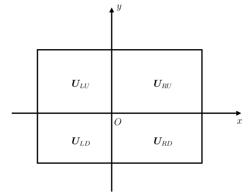
Figure 2.1: The initial data of the 2D Riemann problem at the origin $O$.

Consider the 2D Riemann problem of (1.1) with the initial data as displayed in Fig. 2.1, where four constant states, $\bm{U}_{RU}$ (right-up), $\bm{U}_{LU}$ (left-up), $\bm{U}_{LD}$ (left-down) and $\bm{U}_{RD}$ (right-down) are specified in the first, second, third and fourth quadrants, respectively, and $O$ is the coordinate origin. Denote the largest left-, right-, up- and down-moving speeds of the elementary waves emerging from the initial discontinuities by $S_{L}$, $S_{R}$, $S_{U}$, $S_{D}$, respectively. For instance, $S_{L}$ and $S_{R}$ are given obtained as follows: calculate the largest left- and right-moving wave speeds in the 1D HLL solvers [33] for the two $x$-directional 1D Riemann problems, denoted by $RP{\{\bm{U}_{LU},\bm{U}_{RU}\}}$ and $RP{\{\bm{U}_{LD},\bm{U}_{RD}\}}$, and then minimize two left-moving speeds of those 1D HLL solvers and maximize corresponding two right-moving speeds to give respectively $S_{L}$ and $S_{R}$. Similarly, $S_{D}$ and $S_{U}$ are obtained by considering two $y$-directional 1D Riemann problems denoted by $RP{\{\bm{U}_{LU},\bm{U}_{LD}\}}$ and $RP{\{\bm{U}_{RU},\bm{U}_{RD}\}}$.

In the following, the symbols $(\bm{F}_{1},\bm{F}_{2})$, $(u_{1},u_{2})$, and $(x_{1},x_{2})$ will be replaced with $(\bm{F},\bm{G})$, $(u,v)$, and $(x,y)$, respectively, and we only discuss the case of that $S_{L}<0<S_{R}$ and $S_{D}<0<S_{U}$, because in the case of that $S_{L}$ and $S_{R}$ (or $S_{D}$ and $S_{U}$) have the same sign, our genuinely multidimensional scheme will only call the 1D Riemann solver. Similar to the case of the 1D HLL Riemann solver, we have to derive the intermediate state $\bm{U}^{\ast}$ in the approximate solution of the above Riemann problem and corresponding fluxes $\bm{F}^{\ast}$ and $\bm{G}^{\ast}$. For any given time $T>0$, choose a three-dimensional cuboid $\mathbb{V}_{LRDU}(0,T)$ in the $(x,y,t)$ space as follows: the top and bottom of the cuboid are rectangles with four vertices

$$(TS_{L},TS_{D},0),(TS_{R},TS_{D},0),(TS_{L},TS_{U},0),(TS_{R},TS_{U},0),$$

and

$$(TS_{L},TS_{D},T),(TS_{R},TS_{D},T),(TS_{L},TS_{U},T),(TS_{R},TS_{U},T),$$

respectively. Integrating (1.1) over such cuboid gives

$$\bm{U}^{\ast}\mathscr{A} -\int_{TS_{L}}^{TS_{R}}\int_{TS_{D}}^{TS_{U}}\bm{U}(x,y,0)dydx$$

$$+\int_{0}^{T}\int_{TS_{D}}^{TS_{U}}\bm{F}(\bm{U}(TS_{R},y,0))dydt-\int_{0}^{T}\int_{TS_{D}}^{TS_{U}}\bm{F}(\bm{U}(TS_{L},y,0))dydt$$

$$+\int_{0}^{T}\int_{TS_{L}}^{TS_{R}}\bm{G}(\bm{U}(x,TS_{U},0))dxdt-\int_{0}^{T}\int_{TS_{L}}^{TS_{R}}\bm{G}(\bm{U}(x,TS_{D},0))dxdt=0,$$ (2.1)

where

$$\bm{U}^{\ast}:=\frac{1}{\mathscr{A}}\int_{TS_{D}}^{TS_{U}}\int_{TS_{L}}^{TS_{R}}\bm{U}(x,y,T)dxdy,\ \ \mathscr{A}:=T^{2}(S_{R}-S_{L})(S_{U}-S_{D}).$$

From (2.1), one has

$$\bm{U}^{\ast}: =\frac{1}{\mathscr{A}}\int_{TS_{D}}^{TS_{U}}\int_{TS_{L}}^{TS_{R}}\bm{U}(x,y,T)dxdy=\frac{S_{R}S_{U}\bm{U}_{RU}+S_{L}S_{D}\bm{U}_{LD}-S_{R}S_{D}\bm{U}_{RD}-S_{L}S_{U}\bm{U}_{LU}}{(S_{R}-S_{L})(S_{U}-S_{D})}$$

$$-\frac{S_{U}(\bm{F}_{RU}-\bm{F}_{LU})-S_{D}(\bm{F}_{RD}-\bm{F}_{LD})}{(S_{R}-S_{L})(S_{U}-S_{D})}-\frac{S_{R}(\bm{G}_{RU}-\bm{G}_{RD})-S_{L}(\bm{G}_{LU}-\bm{G}_{LD})}{(S_{R}-S_{L})(S_{U}-S_{D})}.$$ (2.2)

It is shown that the calculation of the intermediate state $\bm{U}^{\ast}$ requires four statuses $\bm{U}_{LD}$, $\bm{U}_{LU}$, $\bm{U}_{RD}$, and $\bm{U}_{RU}$, in other words, $\bm{U}^{\ast}$ contains the genuinely multidimensional information. In the special case of that

$$\bm{U}_{LD}=\bm{U}_{LU},~{}~{}~{}\bm{U}_{RD}=\bm{U}_{RU},$$

one has

$$\bm{F}_{LD}=\bm{F}_{LU},~{}~{}~{}\bm{F}_{RD}=\bm{F}_{RU},~{}~{}~{}\bm{G}_{LD}=\bm{G}_{LU},~{}~{}~{}\bm{G}_{RD}=\bm{G}_{RU},$$

and

$$\bm{U}^{\ast}=\frac{S_{R}\bm{U}_{RD}-S_{L}\bm{U}_{LU}+\bm{F}_{LD}-\bm{F}_{RD}}{S_{R}-S_{L}},$$ (2.3)

which is the same as the intermediate state in the 1D HLL Riemann solver in [33].

Let us turn to obtain the resolved fluxes $\bm{F}^{\ast}$ and $\bm{G}^{\ast}$ for the multidimensional Riemann solver for the case of $S_{L}<0<S_{R}$ and $S_{D}<0<S_{U}$. Integrating respectively the system (1.1) over the left portion and top portion (or the right and bottom portions) of the control volume $\mathbb{V}_{LRDU}(0,T)$ yields

$$\int_{TS_{L}}^{0}\int_{TS_{D}}^{TS_{U}}\bm{U}(x,y,T)dydx =\int_{TS_{L}}^{0}\int_{TS_{D}}^{TS_{U}}\bm{U}(x,y,0)dydx$$

$$~{}~{}~{}~{}~{}-\int_{0}^{T} \int_{TS_{D}}^{TS_{U}}\big{(}\bm{F}(\bm{U}(0,y,t))-\bm{F}(\bm{U}(TS_{L},y,t))\big{)}dydt$$

$$-\int_{0}^{T} \int_{TS_{L}}^{0}\big{(}\bm{G}(\bm{U}(x,TS_{U},t))-\bm{G}(\bm{U}(x,TS_{D},t))\big{)}dxdt,$$ (2.4)

$$\int_{TS_{L}}^{TS_{R}}\int_{0}^{TS_{U}}\bm{U}(x,y,T)dydx =\int_{TS_{L}}^{TS_{R}}\int_{0}^{TS_{U}}\bm{U}(x,y,0)dydx$$

$$-\int_{0}^{T}\int_{0}^{TS_{U}} \big{(}\bm{F}(\bm{U}(TS_{R},y,t))-\bm{F}(\bm{U}(TS_{L},y,t))\big{)}dydt$$

$$-\int_{0}^{T}\int_{TS_{L}}^{TS_{R}} \big{(}\bm{G}(\bm{U}(x,TS_{U},t))-\bm{G}(\bm{U}(x,0,t))\big{)}dxdt.$$ (2.5)

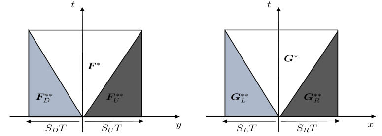
Figure 2.2: Fluxes along the faces $x=0$ (left) and $y=0$ (right) respectively consisting of several different portions.

As shown in the Figure 2.2, the fluxes along the faces $x=0$ (left) and $y=0$ (right) respectively are consisting of several different portions, so that the area integrals in (2.5) on the $x=0$ and $y=0$ faces respectively read as

$$\int_{0}^{T}\int_{TS_{D}}^{TS_{U}}\bm{F}(\bm{U}(0,y,t)) =\frac{T^{2}}{2}\bigg{(}S_{U}\bm{F}_{U}^{\ast\ast}-S_{D}\bm{F}_{D}^{\ast\ast}+(S_{U}-S_{D})\bm{F}^{\ast}\bigg{)},$$ (2.6)

$$\int_{0}^{T}\int_{TS_{L}}^{TS_{R}}\bm{G}(\bm{U}(x,0,t)) =\frac{T^{2}}{2}\bigg{(}S_{R}\bm{G}_{R}^{\ast\ast}-S_{L}\bm{G}_{L}^{\ast\ast}+(S_{G}-S_{L})\bm{G}^{\ast}\bigg{)},$$ (2.7)

where $\bm{F}_{U}^{\ast\ast},\bm{F}_{D}^{\ast\ast},\bm{G}_{R}^{\ast\ast}$, and $\bm{G}_{L}^{\ast\ast}$ are corresponding 1D HLL fluxes in the 1D HLL Riemann solver and have the specific formulations of

$$\bm{F}_{U}^{\ast\ast} =\frac{1}{S_{R}-S_{L}}\bigg{(}S_{R}\bm{F}_{LU}-S_{L}\bm{F}_{RU}+S_{L}S_{R}(\bm{U}_{RU}-\bm{U}_{LU})\bigg{)},$$ (2.8)

$$\bm{F}_{D}^{\ast\ast} =\frac{1}{S_{R}-S_{L}}\bigg{(}S_{R}\bm{F}_{LD}-S_{L}\bm{F}_{RD}+S_{L}S_{R}(\bm{U}_{RD}-\bm{U}_{LD})\bigg{)},$$ (2.9)

$$\bm{G}_{R}^{\ast\ast} =\frac{1}{S_{U}-S_{D}}\bigg{(}S_{U}\bm{G}_{RD}-S_{D}\bm{G}_{RU}+S_{D}S_{U}(\bm{U}_{RU}-\bm{U}_{RD})\bigg{)},$$ (2.10)

$$\bm{G}_{L}^{\ast\ast} =\frac{1}{S_{U}-S_{D}}\bigg{(}S_{U}\bm{G}_{LD}-S_{D}\bm{G}_{LU}+S_{D}S_{U}(\bm{U}_{LU}-\bm{U}_{LD})\bigg{)}.$$ (2.11)

Combining $\eqref{eq43}$ with the relations in (2.4)-(2.11) yields

$$\bm{F}^{\ast} =\frac{1}{S_{U}-S_{D}}\bigg{(}S_{U}\bm{F}_{U}^{\ast\ast}-S_{D}\bm{F}_{D}^{\ast\ast}-\frac{2S_{L}S_{R}}{S_{R}-S_{L}}(\bm{G}_{RU}-\bm{G}_{RD}-\bm{G}_{LU}+\bm{G}_{LD})\bigg{)},$$ (2.12)

$$\bm{G}^{\ast} =\frac{1}{S_{R}-S_{L}}\bigg{(}S_{R}\bm{G}_{R}^{\ast\ast}-S_{L}\bm{G}_{L}^{\ast\ast}-\frac{2S_{D}S_{U}}{S_{U}-S_{D}}(\bm{F}_{RU}-\bm{F}_{RD}-\bm{F}_{LU}+\bm{F}_{LD})\bigg{)}.$$ (2.13)

For all other cases with the certain signs (either positive or negative) of $S_{L},S_{R},S_{D},S_{U}$, different from the case of $S_{L}<0<S_{R}$ and $S_{D}<0<S_{U}$, we can similarly evaluate the above area integrals on the $x=0$ and $y=0$ faces, and get the fluxes $\bm{F}^{\ast}$ and $\bm{G}^{\ast}$ in the multidimensional Riemann solver by (2.4) and (2.5). The multidimensional fluxes can be generalized for all situations by setting [33]

$$S_{L}^{-}=\min(S_{L},0),~{}~{}S_{R}^{+}=\max(S_{R},0),~{}~{}S_{D}^{-}=\min(S_{D},0),~{}~{}S_{U}^{+}=\max(S_{U},0).$$ (2.14)

If denoting the 2D HLL fluxes as $\bm{F}^{\text{2D-HLL}}$ and $\bm{G}^{\text{2D-HLL}}$ in $x$- and $y$-directions respectively, then one has their explicit forms

$$\begin{aligned} &\bm{F}^{\text{2D-HLL}}(\bm{U}_{LD},\bm{U}_{LU},\bm{U}_{RD},\bm{U}_{RU})\\ =&\frac{1}{S_{U}^{+}-S_{D}^{-}}\bigg{(}S_{U}^{+}\bm{F}_{U}^{\ast\ast}-S_{D}^{-}\bm{F}_{D}^{\ast\ast}-\frac{2S_{L}^{-}S_{R}^{+}}{S_{R}^{+}-S_{L}^{-}}(\bm{G}_{RU}-\bm{G}_{RD}-\bm{G}_{LU}+\bm{G}_{LD})\bigg{)},\end{aligned}$$ (2.15)

$$\begin{aligned} &\bm{G}^{\text{2D-HLL}}(\bm{U}_{LD},\bm{U}_{LU},\bm{U}_{RD},\bm{U}_{RU})\\ =&\frac{1}{S_{R}^{+}-S_{L}^{-}}\bigg{(}S_{R}^{+}\bm{G}_{R}^{\ast\ast}-S_{L}^{-}\bm{G}_{L}^{\ast\ast}-\frac{2S_{D}^{-}S_{U}^{+}}{S_{U}^{+}-S_{D}^{-}}(\bm{F}_{RU}-\bm{F}_{RD}-\bm{F}_{LU}+\bm{F}_{LD})\bigg{)}.\end{aligned}$$ (2.16)

Now we begin to study the PCP property of the multidimensional HLL Riemann solver, which means that the resolved state $\bm{U}^{\ast}$ in the multidimensional Riemann solver is admissible. Only the case of $S_{L}<0<S_{R},S_{D}<0<S_{U}$ needs to be discussed here, since the other situations (except for the non-trivial case of $S_{L}<0<S_{R},S_{D}<0<S_{U}$) produce the 1D resolved state which can be easily proved to be PCP according to [19].

Before that, we first give the specific definition of wave speeds $S_{L},S_{R},S_{D},S_{U}$. There exist several different ways to define the wave speeds in the 1D HLL-type Riemann solvers, see e.g. [5, 14, 9]. If letting $\lambda_{A}^{(1)}(\bm{U}_{LD})$ and $\lambda_{A}^{(4)}(\bm{U}_{LD})$ denote the smallest and largest eigenvalues of Jacobian matrix $\partial\bm{F}/\partial\bm{U}(\bm{U}_{LD})$, and making corresponding definitions for the other states in the $x$- and $y$-directions similarly, then the wave speeds $S_{L},S_{R},S_{D}$ and $S_{U}$ are given by

$$S_{L}=\alpha\min\big{(}\lambda_{A}^{(1)}(\bm{U}_{LD}),\lambda_{A}^{(1)}(\bm{U}_{RD}),\lambda_{A}^{(1)}(\bm{U}_{LU}),\lambda_{A}^{(1)}(\bm{U}_{RU})\big{)},$$ (2.17)

$$S_{R}=\alpha\max\big{(}\lambda_{A}^{(4)}(\bm{U}_{LD}),\lambda_{A}^{(4)}(\bm{U}_{RD}),\lambda_{A}^{(4)}(\bm{U}_{LU}),\lambda_{A}^{(4)}(\bm{U}_{RU})\big{)},$$

$$S_{D}=\alpha\min\big{(}\lambda_{B}^{(1)}(\bm{U}_{LD}),\lambda_{B}^{(1)}(\bm{U}_{RD}),\lambda_{B}^{(1)}(\bm{U}_{LU}),\lambda_{B}^{(1)}(\bm{U}_{RU})\big{)},$$

$$S_{U}=\alpha\max\big{(}\lambda_{B}^{(4)}(\bm{U}_{LD}),\lambda_{B}^{(4)}(\bm{U}_{RD}),\lambda_{B}^{(4)}(\bm{U}_{RU}),\lambda_{B}^{(4)}(\bm{U}_{LU})\big{)},$$

where $\alpha\geq 1$ is to be determined later. The PCP property of the multidimensional HLL Riemann solver with (2.17) can be obtained as follows.

Theorem 2.1.

The intermediate state $\bm{U}^{\ast}$ in (2.2) obtained from the multidimensional HLL Riemann solver is admissible, i.e.

$$D^{\ast}>0,~{}~{}E^{\ast}>0,~{}~{}(E^{\ast})^{2}-(D^{\ast})^{2}-|\bm{m}^{\ast}|^{2}>0,$$

if the wave speeds $S_{L},S_{R},S_{D},S_{U}$ are taken as (2.17) with $\alpha=2$.

Proof.

Let us assume $S_{L}<0<S_{R},S_{D}<0<S_{U}$. Rewrite $\bm{U}^{\ast}$ as

$$\bm{U}^{\ast}=\frac{1}{\mathscr{B}}\bigg{(}S_{L}S_{D}\bm{H}_{LD}-S_{R}S_{D}\bm{H}_{RD}-S_{L}S_{U}\bm{H}_{LU}+S_{R}S_{U}\bm{H}_{RU}\bigg{)},$$

with $\mathscr{B}=(S_{R}-S_{L})(S_{U}-S_{D})$ and

$$\bm{H}_{LD}=\bm{U}_{LD}-\frac{1}{S_{L}}\bm{F}_{LD}-\frac{1}{S_{D}}\bm{G}_{LD},~{}~{}\bm{H}_{RD}=\bm{U}_{RD}-\frac{1}{S_{R}}\bm{F}_{RD}-\frac{1}{S_{D}}\bm{G}_{RD},$$

$$\bm{H}_{LU}=\bm{U}_{LU}-\frac{1}{S_{L}}\bm{F}_{LU}-\frac{1}{S_{U}}\bm{G}_{LU},~{}~{}\bm{H}_{RU}=\bm{U}_{RU}-\frac{1}{S_{R}}\bm{F}_{RU}-\frac{1}{S_{U}}\bm{G}_{RU}.$$

Because $\bm{U}^{\ast}$ is a convex combination of $\bm{H}_{LD},\bm{H}_{RD}$, $\bm{H}_{LU},\bm{H}_{RU}$, it is sufficient to have those $\bm{H}$-terms to be in the admissible set $\mathcal{G}$. As an example, consider the term $\bm{H}_{LD}$, which can be decomposed into two parts as follows

$$\bm{H}_{LD}=\bm{U}_{LD}-\frac{1}{S_{L}}\bm{F}_{LD}-\frac{1}{S_{D}}\bm{G}_{LD}=\frac{1}{2}\bigg{(}\bm{U}_{LD}-\frac{2}{S_{L}}\bm{F}_{LD}\bigg{)}+\frac{1}{2}\bigg{(}\bm{U}_{LD}-\frac{2}{S_{D}}\bm{G}_{LD}\bigg{)}.$$

The properties (ii) and (iii) in Lemma 1.2 show the admissibility of $\bm{U}_{LD}-\frac{2}{S_{L}}\bm{F}_{LD}$ and $\bm{U}_{LD}-\frac{2}{S_{D}}\bm{G}_{LD}$ so is $\bm{H}_{LD}$. Using the similar way can shows that other $\bm{H}$-terms are also admissible. The proof is completed. ∎

3 Numerical scheme

This section presents the first-order accurate PCP finite volume schemes with multidimensional HLL Riemann solver for the special RHD equations (1.1).

Assume that she computational domain is divided into $N\times M$ rectangular cells: $I_{i,j}=(x_{i-\frac{1}{2}},x_{i+\frac{1}{2}})\times(y_{j-\frac{1}{2}},y_{j+\frac{1}{2}})$ with the step-sizes $\Delta x_{i}=x_{i+\frac{1}{2}}-x_{i-\frac{1}{2}},\Delta y_{j}=y_{j+\frac{1}{2}}-y_{j-\frac{1}{2}}$ for $i=1,\cdots,N;j=1,\cdots,M$, and that the time interval $\{t>0\}$ is discretized as: $t_{n+1}=t_{n}+\Delta t^{n}$, $n=0,1,2,\cdots$, where $\Delta t^{n}$ is the time step size at $t=t_{n}$, determined by the CFL type condition

$$\Delta t^{n}\leq\sigma\min\limits_{i,j}\left\{\frac{\Delta x_{i}}{\max\big{(}|\lambda_{A}^{(1)}(\overline{\bm{U}}_{ij}^{n})|,|\lambda_{A}^{(4)}(\overline{\bm{U}}_{ij}^{n})|\big{)}},\frac{\Delta y_{j}}{\max\big{(}|\lambda_{B}^{(1)}(\overline{\bm{U}}_{ij}^{n})|,|\lambda_{B}^{(4)}(\overline{\bm{U}}_{ij}^{n})|\big{)}}\right\},$$ (3.1)

here the CFL number $\sigma\leq 1$, and $\overline{\bm{U}}_{ij}^{n}$ is the (approximate) cell average value of $\bm{U}$ at $t_{n}$ over the cell $I_{i,j}$.

For the RHD system (1.1), the finite volume scheme with the Euler forward time discretization can be formulated as follows

$$\overline{\bm{U}}_{ij}^{n+1}=\overline{\bm{U}}_{ij}^{n}-\frac{\Delta t^{n}}{\Delta x_{i}}\big{(}\widehat{\bm{F}}_{i+\frac{1}{2},j}-\widehat{\bm{F}}_{i-\frac{1}{2},j}\big{)}-\frac{\Delta t^{n}}{\Delta y_{j}}\big{(}\widehat{\bm{G}}_{i,j+\frac{1}{2}}-\widehat{\bm{G}}_{i,j-\frac{1}{2}}\big{)},$$ (3.2)

where $\widehat{\bm{F}}$ and $\widehat{\bm{G}}$ are the numerical fluxes evaluated at zone faces corresponding to the $x$- and $y$-directions, respectively. For the genuinely multidimensional scheme, by means of Figure 2.2, the fluxes $\widehat{\bm{F}}$ and $\widehat{\bm{G}}$ should be contributed by the 1D Riemann solver at the center of the zone face and the 2D Riemann solver at the corners of that face. In our 2D scheme, the flux $\widehat{\bm{F}}_{i+\frac{1}{2},j}$ consists of three parts: $\bm{F}_{i+\frac{1}{2},j}^{\text{1D-HLL}}$ computed from the 1D HLL Riemann solver and $\bm{F}_{i+\frac{1}{2},j\pm\frac{1}{2}}^{\text{2D-HLL}}$ computed from the 2D HLL Riemann solver, where

$$\bm{F}^{\text{1D-HLL}}_{i+\frac{1}{2},j}=\bm{F}^{\text{1D-HLL}}(\bm{U}_{i+\frac{1}{2},j}^{L},\bm{U}_{i+\frac{1}{2},j}^{R}),$$ (3.3)

$$\bm{F}^{\text{2D-HLL}}_{i+\frac{1}{2},j\pm\frac{1}{2}}=\bm{F}^{\text{2D-HLL}}\big{(}\bm{U}^{LD}_{i+\frac{1}{2},j\pm\frac{1}{2}},\bm{U}^{RD}_{i+\frac{1}{2},j\pm\frac{1}{2}},\bm{U}^{LU}_{i+\frac{1}{2},j\pm\frac{1}{2}},\bm{U}^{RU}_{i+\frac{1}{2},j\pm\frac{1}{2}}\big{)},$$

with $\bm{U}_{i+\frac{1}{2},j}^{L},\bm{U}_{i+\frac{1}{2},j}^{R}$ being the left and right limited approximations of $\bm{U}$ at the center of the edge $x=x_{i+\frac{1}{2}}$, and $\bm{U}^{LD}_{i+\frac{1}{2},j\pm\frac{1}{2}},\bm{U}^{RD}_{i+\frac{1}{2},j\pm\frac{1}{2}},\bm{U}^{LU}_{i+\frac{1}{2},j\pm\frac{1}{2}},\bm{U}^{RU}_{i+\frac{1}{2},j\pm\frac{1}{2}}$ being the left-down, right-down, left-up and right-up limited approximations of $\bm{U}$ at the node $(x_{i+\frac{1}{2}},y_{j\pm\frac{1}{2}})$. Those limited approximations can be obtained by using the initial reconstruction technique and $\{\overline{\bm{U}}_{ij}^{n}\}$ respectively. For example, for the first-order accurate scheme, they can be calculated from the reconstructed piecewise constant function

$$\bm{U}_{i+\frac{1}{2},j}^{L}=\overline{\bm{U}}_{ij},~{}~{}~{}~{}~{}~{}~{}~{}\bm{U}_{i+\frac{1}{2},j}^{R}=\overline{\bm{U}}_{i+1,j},~{}~{}~{}~{}~{}\bm{U}^{LD}_{i+\frac{1}{2},j+\frac{1}{2}}=\overline{\bm{U}}_{ij},$$ (3.4)

$$\bm{U}^{RD}_{i+\frac{1}{2},j+\frac{1}{2}}=\overline{\bm{U}}_{i+1,j},~{}\bm{U}^{LU}_{i+\frac{1}{2},j+\frac{1}{2}}=\overline{\bm{U}}_{i,j+1},~{}~{}\bm{U}^{RU}_{i+\frac{1}{2},j+\frac{1}{2}}=\overline{\bm{U}}_{i+1,j+1}.$$

In summary, our final numerical fluxes $\widehat{\bm{F}}$ and $\widehat{\bm{G}}$ are given as follows

$$\widehat{\bm{F}}_{i+\frac{1}{2},j} =\frac{\Delta t^{n}}{2\Delta y_{j}}\big{(}S_{U,i+\frac{1}{2},j-\frac{1}{2}}^{+}\bm{F}^{\text{2D-HLL}}_{i+\frac{1}{2},j-\frac{1}{2}}-S_{D,i+\frac{1}{2},j+\frac{1}{2}}^{-}\bm{F}^{\text{2D-HLL}}_{i+\frac{1}{2},j+\frac{1}{2}}\big{)}$$

$$~{}~{}~{}+\left(1-\frac{\Delta t^{n}}{2\Delta y_{j}}(S_{U,i+\frac{1}{2},j-\frac{1}{2}}^{+}-S_{D,i+\frac{1}{2},j+\frac{1}{2}}^{-})\right)\bm{F}_{i+\frac{1}{2},j}^{\text{1D-HLL}},$$ (3.5)

$$\widehat{\bm{G}}_{i,j+\frac{1}{2}} =\frac{\Delta t^{n}}{2\Delta x_{i}}\big{(}S_{R,i-\frac{1}{2},j+\frac{1}{2}}^{+}\bm{G}^{\text{2D-HLL}}_{i-\frac{1}{2},j+\frac{1}{2}}-S_{L,i+\frac{1}{2},j+\frac{1}{2}}^{-}\bm{G}^{\text{2D-HLL}}_{i+\frac{1}{2},j+\frac{1}{2}}\big{)}$$

$$~{}~{}~{}+\left(1-\frac{\Delta t^{n}}{2\Delta x_{i}}(S_{R,i-\frac{1}{2},j+\frac{1}{2}}^{+}-S_{L,i+\frac{1}{2},j+\frac{1}{2}}^{-})\right)\bm{G}_{i,j+\frac{1}{2}}^{\text{1D-HLL}},$$ (3.6)

where $S_{L}^{-},S_{R}^{+},S_{D}^{-},S_{U}^{+}$ are defined in (2.14).

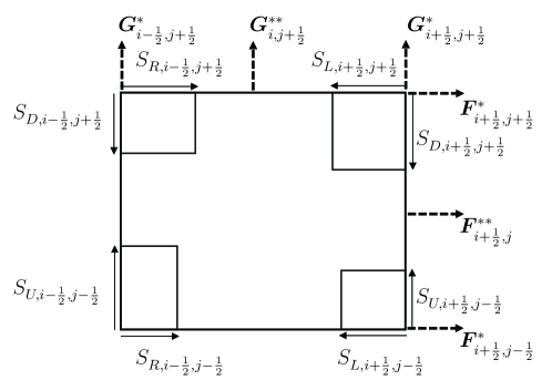
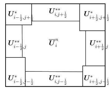
Figure 3.1: Illustration for the numerical fluxes (left) and approximate solution (right) for the numerical scheme (3.2).

Now, let us discuss the PCP property of the scheme (3.2) with the numerical fluxes (3.5) and (3.6). Following the design of the 1D and 2D HLL Riemann solvers, under the CFL condition (3.1) with $\sigma\leq\frac{1}{2}$, the scheme (3.2) can be written as an exact integration of those two approximate Riemann solvers over the cell $I_{i,j}$. For the the non-trivial case: $S_{L}<0<S_{R},S_{D}<0<S_{U}$, the updated solution $\overline{\bm{U}}_{ij}^{n+1}$ can be reformulated as a convex combination of nine terms: $\overline{\bm{U}}_{ij}^{n},\bm{U}_{i-\frac{1}{2},j-\frac{1}{2}}^{\ast},\bm{U}_{i+\frac{1}{2},j-\frac{1}{2}}^{\ast},\bm{U}_{i-\frac{1}{2},j+\frac{1}{2}}^{\ast},\bm{U}_{i-\frac{1}{2},j+\frac{1}{2}}^{\ast}$ and $\bm{U}_{i-\frac{1}{2},j}^{\ast\ast},\bm{U}_{i+\frac{1}{2},j}^{\ast\ast},\bm{U}_{i,j-\frac{1}{2}}^{\ast\ast},\bm{U}_{i,j+\frac{1}{2}}^{\ast\ast}$, which is illustrated in Figure 3.1. The terms with superscript “$\ast$” are the approximate Riemann solutions obtained from the multidimensional HLL Riemann solver and the terms with superscript “$\ast\ast$” are the approximate Riemann solutions obtained from the 1D HLL Riemann solver. Each term in the convex combination is admissible, see Section 2, and thus the numerical solution $\overline{\bm{U}}_{ij}^{n+1}$ to the first-order scheme (3.2) with (3.4) is also admissible. We conclude such result in the following theorem.

Theorem 3.1.

If $\{\overline{\bm{U}}_{ij}^{n}\in\mathcal{G},\forall i=1,\cdots,N;j=1,\cdots,M\}$ and the wave speeds $S_{D},S_{U},S_{L},S_{R}$ are estimated by (2.17), then $\overline{\bm{U}}_{ij}^{n+1}$ obtained by the first-order scheme (3.2) with (3.4) and the multidimensional Riemann solver belongs to the admissible state set $\mathcal{G}$ under the time step restriction (3.1) with $\sigma\leq\frac{1}{2}$.

4 Numerical tests

This section conducts several numerical experiments on the 2D ultra-relativistic RHD problems with large Lorentz factor, or strong discontinuities, or low rest-mass density or pressure, to verify the accuracy, robustness, and effectiveness of the present PCP scheme. It is worth remarking that those ultra-relativistic RHD problems seriously challenge the numerical scheme. Unless otherwise stated, all the computations are restricted to the equation of state (1.3) with the adiabatic index $\Gamma=5/3$, and the time step size $\Delta t^{n}$ determined by (3.1) with the CFL number $\sigma=0.45$.

Example 4.1 (Sine wave propagation).

This problem is used to test the accuracy of our PCP finite volume scheme. Its exact solution is

$$(\rho,u,v,p)(t,x,y)=(1+\delta\sin(2\pi(x+y-0.99\sqrt{2}t)),0.99/\sqrt{2},0.99/\sqrt{2},0.01),\ t\geq 0$$

which describe an RHD sine wave propagating periodically in the domain $\Omega=(0,1)\times(0,1)$ at an angle $45^{\circ}$ with the $x$-axis. The computational domain is divided into $N\times N$ uniform cells, $\delta=0.99999$, and the periodic boundary conditions are specified on the boundary of $\Omega$. Table 4.1 lists the $\ell^{1},\ell^{2}$ and $\ell^{\infty}$ errors at $t=0.1$ and orders of convergence obtained from our first-order multidimensional PCP scheme. The results show the expected PCP performance.

$N$	$\ell^{1}$ error	$\ell^{1}$ order	$\ell^{2}$ error	$\ell^{2}$ order	$\ell^{\infty}$ error	$\ell^{\infty}$ order
20	5.521E-02	—–	6.146E-02	—–	8.683E-02	—–
40	2.705E-02	1.029	3.003E-02	1.033	4.241E-02	1.034
80	1.338E-02	1.016	1.486E-02	1.015	2.101E-02	1.013
160	6.710E-03	0.996	7.452E-03	0.996	1.054E-02	0.996
320	3.359E-03	0.998	3.731E-03	0.998	5.277E-03	0.998

Table 4.1: Example 4.1: Errors and orders of convergence for the rest-mass density $\rho$ at $t=0.1$ obtained by using the first-order PCP scheme with the mesh of $N\times N$ uniform cells.

Example 4.2 (Relativistic isentropic vortex).

It is a 2D relativistic isentropic vortex problem constructed first in [19], where the vortex in the space-time coordinate system $(t,x,y)$ moves with a constant speed of magnitude $w$ in $(-1,-1)$ direction. The time-dependent solution $(\rho,u,v,p)$ at time $t\geq 0$ is given as follows

$$\rho=(1-\alpha e^{1-r^{2}})^{\frac{1}{\Gamma-1}},\quad p=\rho^{\Gamma},$$

$$u=\frac{1}{1-\frac{w(u_{0}+v_{0})}{\sqrt{2}}}\left[\frac{u_{0}}{\gamma}-\frac{w}{\sqrt{2}}+\frac{\gamma w^{2}}{2(\gamma+1)}(u_{0}+v_{0})\right],$$

$$v=\frac{1}{1-\frac{w(u_{0}+u_{0})}{\sqrt{2}}}\left[\frac{v_{0}}{\gamma}-\frac{w}{\sqrt{2}}+\frac{\gamma w^{2}}{2(\gamma+1)}(u_{0}+v_{0})\right],$$

where

$$\gamma=\frac{1}{\sqrt{1-w^{2}}},\quad r=\sqrt{x_{0}^{2}+y_{0}^{2}},\quad(u_{0},v_{0})=(-y_{0},x_{0})f,$$

$$\alpha=\frac{(\Gamma-1)}{8\Gamma}\pi^{2}\epsilon^{2},\quad\beta=\dfrac{\Gamma^{2}\alpha e^{1-r^{2}}}{2\Gamma-1-\Gamma\alpha e^{1-r^{2}}},\quad f=\sqrt{\frac{\beta}{1+\beta r^{2}}},$$

$$x_{0}=x+\frac{\gamma-1}{2}(x+y)+\frac{\gamma tw}{\sqrt{2}},~{}~{}y_{0}=y+\frac{\gamma-1}{2}(x+y)+\frac{\gamma tw}{\sqrt{2}}.$$

Our computations are performed in the domain $\Omega=(-5,5)\times(-5,5)$ with the adiabatic index $\Gamma=1.4$, $w=0.5\sqrt{2}$, the vortex strength $\epsilon=10.0828$, and the periodic boundary conditions. In this case, the lowest density and lowest pressure are $7.8\times 10^{-15}$ and $1.78\times 10^{-20}$, respectively.

Table 4.2 gives the errors of the rest-mass density at $t=1$ and the orders of convergence. It is clear to see that our multidimensional PCP scheme achieves the expected accuracy and preserves the positivity of the density and pressure simultaneously.

$N$	$\ell^{1}$ error	$\ell^{1}$ order	$\ell^{2}$ error	$\ell^{2}$ order	$\ell^{\infty}$ error	$\ell^{\infty}$ order
20	1.566E-02	—–	5.026E-02	—–	3.285E-01	—–
40	8.881E-03	0.818	2.855E-02	0.816	2.061E-01	0.672
80	4.779E-03	0.894	1.550E-02	0.881	1.189E-01	0.794
160	2.495E-03	0.938	8.212E-03	0.916	6.644E-02	0.839
320	1.280E-03	0.963	4.260E-03	0.947	3.528E-02	0.913

Table 4.2: Example 4.2: Errors and orders of convergence for rest-mass density at $t=1$ obtained by using the first-order scheme with the mesh of $N\times N$ uniform cells.

Example 4.3 (Explosion).

It is used to test the multi-dimensionality of our scheme. Initially, the rest fluid with a unit rest-mass density is in the domain $\Omega=(-0.5,0.5)\times(-0.5,0.5)$. The pressure is set as 20 inside a circle of radius 1/10, while a smaller pressure of 0.1 is given all over outside the circle. Figure 4.1 plots the contours and cut lines along $y$-axis and $y=x$ of the rest-mass density at $t=0.1$ obtained by using our scheme with the multidimensional Riemann solver on the mesh of $64\times 64$ uniform cells. For a comparison, Figures 4.2 gives the numerical solutions obtained by using the scheme with the 1D Riemann solver. It can be clearly seen from them that the results obtained by our scheme with the 2D Riemann solver preserve the spherical symmetry better.

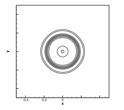
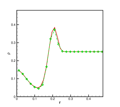
Figure 4.1: Example 4.3: The rest-mass density at $t=0.1$ obtained our scheme. Left: The contours with eight equally spaced contour lines; right: the cut lines of $\rho$ at $y$-axis (solid line) and $y=x$ (dashed line with the symbol “$\diamond$”).

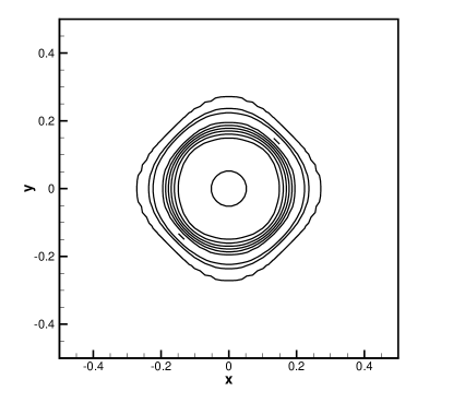
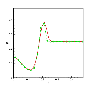
Figure 4.2: Same as Figure 4.1, except for the 1D HLL Riemann solver.

Example 4.4 (Riemann problem I).

The example solves the 2D Riemann problem [49, 41]. The initial data are given by

$$(\rho,u,v,p)(0,x,y)=\begin{cases}(0.1,0,0,0.01),&x>0,~{}y>0,\\ (0.1,0.99,0,1),&x<0,~{}y>0,\\ (0.5,0,0,1),&x<0,~{}y<0,\\ (0.1,0,0.99,1),&x>0,~{}y<0,\end{cases}$$

where both the left and bottom discontinuities are the contact discontinuities with a jump in the transverse velocity, while both the right and top discontinuities are not simple waves. It is necessary to remark that this case is different from that in [47].

The computational domain $\Omega$ is taken as $(-1,1)\times(-1,1)$ and is divided into a uniform mesh with $400\times 400$ cells. Figure 4.3 displays the contours of the rest-mass density logarithm $\ln\rho$ and the pressure logarithm $\ln p$ at $t=0.8$ obtained by using the first-order multidimensional PCP scheme. We can see that the four initial discontinuities interact each other and form two reflected curved shock waves, an elongated jet-like spike. It is worth mentioning that a non-PCP scheme fails when simulating this problem.

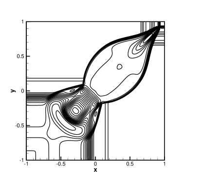
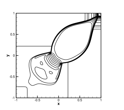
Figure 4.3: Example 4.4: The contours of the density logarithm $\ln\rho$ (left) and the pressure logarithm $\ln p$ (right) at $t=0.8$. 30 equally spaced contour lines are used.

Example 4.5 (Riemann problem II).

The initial data of the second Riemann problem are

$$(\rho,u,v,p)(0,x,y)=\begin{cases}(0.1,0,0,20),&x>0,~{}y>0,\\ (\widetilde{\rho},\widetilde{u},0,0.05),&x<0,~{}y>0,\\ (0.01,0,0,0.05),&x<0,~{}y<0,\\ (\widetilde{\rho},0,\widetilde{u},0.05),&x>0,~{}y<0,\end{cases}$$

with $\widetilde{\rho}=0.00414329639576$ and $\widetilde{u}=0.9946418833556542$, In this problem, the left and lower initial discontinuities are the contact discontinuities, while the upper and right are shock waves with a speed of $-0.66525606186639$. As the time increases, the maximal value of the fluid velocity becomes very large and close to the speed of light, which leads to the numerical simulation more challenging. Figure 4.4 displays the contours of the rest-mass density logarithm $\ln\rho$ and the pressure logarithm $\ln p$ at $t=0.8$ obtained by using the first-order PCP scheme with the multidimensional HLL Riemann solver on the mesh of $400\times 400$ uiniform cells. for $\Omega=(-1,1)\times(-1,1)$. The interaction of four initial discontinuities results in the distortion of the initial shock waves and the formation of a “mushroom cloud” starting from the point (0,0) and expanding to the left bottom region.

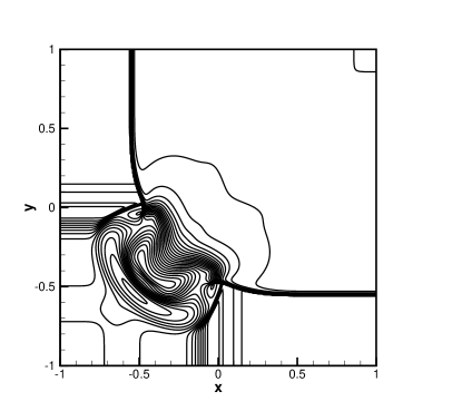
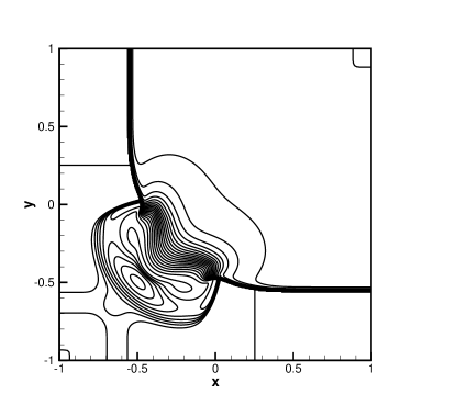
Figure 4.4: Example 4.5: The contours of the density logarithm $\ln\rho$ (left) and the pressure logarithm $\ln p$ (right) at $t=0.8$. 25 equally spaced contour lines are shown.

Example 4.6 (Relativistic jets).

The last example is to simulate two high-speed relativistic jet flows [41], which are ubiquitous in the extragalactic radio sources associated with the active galactic nuclei, and the most compelling case for a special relativistic phenomenon. It is very challenging to simulate such jet flows because there may appear the strong relativistic shock waves, shear waves, interface instabilities, and ultra-relativistic regions, as well as high speed jets etc.

First, we consider a pressure-matched hot jet model, in which the relativistic effects from the large beam internal energies are important and comparable to the effects from the fluid velocity near the speed of light because the classical beam Mach number $M_{b}$ is near the minimum Mach number for given beam speed $v_{b}$. Initially, the computational domain $(0,12)\times(0,30)$ is filled with a static uniform medium with an unit rest-mass density, and a light relativistic jet is injected in the $y$-direction through the inlet part $|x|\leq 0.5$ on the bottom boundary $(y=0)$ with a high speed $v_{b}$, a rest-mass density of 0.01, and a pressure equal to the ambient pressure. The fixed inflow beam condition is specified on the nozzle $\{y=0,|x|\leq 0.5\}$, the reflecting boundary condition is specified at $x=0$, whereas the outflow boundary conditions are on other boundaries. The following three different configurations are considered:

1. $v_{b}=0.99$ and $M_{b}=1.72$, corresponding to the case of $\gamma\approx 7.089$ and $M_{r}\approx 9.971$.

2. $v_{b}=0.999$ and $M_{b}=1.72$, corresponding to the case of $\gamma\approx 22.366$ and $M_{r}\approx 31.316$.

3. $v_{b}=0.9999$ and $M_{b}=1.72$, corresponding to the case of $\gamma\approx 70.712$ and $M_{r}\approx 98.962$.

Here $M_{r}:=M_{b}\gamma/\gamma_{s}$ denotes the relativistic Mach number with $\gamma_{s}=1/\sqrt{1-c_{s}^{2}}$ being the Lorentz factor associated with the local sound speed.

As $v_{b}$ becomes much closer to the speed of light, the simulation of the jet becomes more challenging. Figures 4.5 and 4.6 display the schlieren images of the rest-mass density logarithm $\ln\rho$ and the pressure logarithm $\ln p$ within the domain $[-12,12]\times[0,30]$ at $t=30$ obtained by using the first order scheme with multidimensional HLL Riemann solver with $240\times 600$ uniform cells for the computational domain $(0,12)\times(0,30)$.

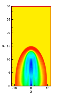
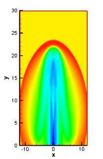
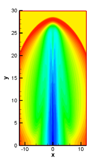
Figure 4.5: Example 4.6: Schlieren images of rest-mass density logarithm $\ln\rho$ at $t=30$ for the hot jet model obtained by the first order scheme with $240\times 600$ uniform cells. From left to right: configurations (i), (ii) and (iii).

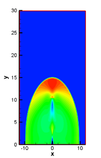
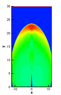
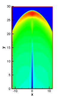
Figure 4.6: Same as Figure 4.5 except for the pressure logarithm $\ln p$.

Next, we consider the pressure-matched highly supersonic jet model, also called as the cold model, in which the relativistic effects from the large beam speed dominate, so that there exists an important difference between the hot and cold relativistic jets. The setups are the same as the above hot jet model, except for that the rest-mass density of the inlet jet becomes 0.1. The computational domain is taken as $(0,12)\times(0,25)$, and again three different configurations are considered here:

1. $v_{b}=0.99$ and $M_{b}=50$, corresponding to the case of $\gamma\approx 7.088$ and $M_{r}\approx 354.371$.

2. $v_{b}=0.999$ and $M_{b}=50$, corresponding to the case of $\gamma\approx 22.366$ and $M_{r}\approx 1118.090$.

3. $v_{b}=0.9999$ and $M_{b}=500$, corresponding to the case of $\gamma\approx 70.712$ and $M_{r}\approx 35356.152$.

Figures 4.7 and 4.8 show the schlieren images of the rest-mass density logarithm $\ln\rho$ and the pressure logarithm $\ln p$ within the domain $[-12,12]\times[0,25]$, obtained by using the first order multidimensional HLL scheme with $240\times 500$ uniform cells for the computational domain $(0,12)\times(0,25)$.

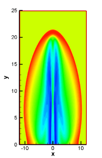
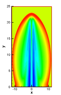
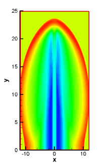
Figure 4.7: Example 4.6: Schlieren images of rest-mass density logarithm $\ln\rho$ for the cold jet model obtained by the first order scheme with $240\times 500$ uniform cells. From left to right: configurations (i) at $t=30$, (ii) at $t=25$, and (iii) at $t=23$.

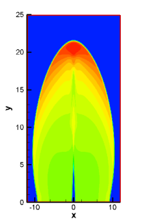
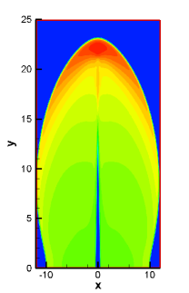
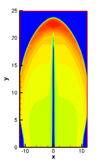
Figure 4.8: Same as Figure 4.7 except for the pressure logarithm $\ln p$.

5 Conclusion

This paper proposed a finite volume scheme based on the multidimensional HLL Riemann solver for the 2D special relativistic hydrodynamics and then studied its PCP property (i.e., preserving the positivity of the rest-mass density and the pressure and the boundness of the fluid velocity). We first proved that the intermediate states in the 1D HLL Riemann solver were PCP when the HLL wave speeds were estimated suitably, and further obtain the PCP property of the intermediate states obtained from the multidimensional HLL Riemann solver in a similar way. Then we developed the first-order accurate PCP finite volume scheme with the multidimensional HLL Riemann solver and forward Euler time discretization. Finally, several 2D numerical experiments were conducted to demonstrate the accuracy and the effectiveness of the proposed PCP scheme in solving the special RHD problems involving large Lorentz factor, or low rest-mass density or low pressure or strong discontinuities, etc. It is worth to remark that the further development of the high-order accurate PCP genuinely multidimensional scheme to higher-order of accuracy seems non-trivial, since some different coefficients have been involved in the numerical fluxes, see (3.5) and (3.6), so that it is too difficult to rewrite a high-order scheme as a convex combination of several first-order like schemes. One possible way to overcome such difficulty is to design a PCP flux-limiter and then modify the numerical flux to achieve the PCP property of the high-order scheme, see e.g. [45].

Appendix Appendix A Proof of Lemma 1.2

This appendix proves Lemma 1.2 presented in Section 1 in a slightly different way from [39].

(i) For any positive number $\kappa$, let $(D^{\kappa},\bm{m}^{\kappa},E^{\kappa})^{T}=\bm{U}^{\kappa}:=\kappa\bm{U}$. Since $\bm{U}\in\mathcal{G}$, it is easy to verify

$$D^{\kappa}=\kappa D>0,\ \ E^{\kappa}-\sqrt{(D^{\kappa})^{2}+|\bm{m}^{\kappa}|^{2}}=\kappa\big{(}E-\sqrt{D^{2}+|\bm{m}|^{2}}\big{)}>0,$$

which leads to admissibility of $\kappa\bm{U}$.

(ii) The convexity of $\mathcal{G}$ shows

$$\frac{a_{1}}{a_{1}+a_{2}}\bm{U}_{1}+\frac{a_{2}}{a_{1}+a_{2}}\bm{U}_{2}\in\mathcal{G},$$

for any $a_{1},a_{2}>0$ and $\bm{U}_{1},\bm{U}_{2}\in\mathcal{G}$. Combining it with the conclusion in (i) yields

$$a_{1}\bm{U}_{1}+a_{2}\bm{U}_{2}\in\mathcal{G}.$$

(iii) For simplicity, denote

$$(D^{\alpha},\bm{m}_{i}^{\alpha},E^{\alpha})^{T}=\bm{U}^{\alpha}: =\alpha\bm{U}-\bm{F}_{i}(\bm{U}),$$

$$(D^{\beta},\bm{m}_{i}^{\beta},E^{\beta})^{T}=\bm{U}^{\beta}: =-\beta\bm{U}+\bm{F}_{i}(\bm{U}).$$

For the state $\bm{U}^{\alpha}$ with $\alpha\geq\lambda_{i}^{(4)}(\bm{U})$, we can get

$$D^{\alpha} =D(\alpha-u_{i})\geq D\big{(}\lambda_{i}^{(4)}(\bm{U})-u_{i}\big{)}>0,$$

$$E^{\alpha} =E(\alpha-u_{i})-pu_{i}\geq E\big{(}\lambda_{i}^{(4)}(\bm{U})-u_{i}\big{)}-pu_{i}$$

$$=\frac{p\gamma^{2}}{c_{s}^{2}}\bigg{(}\big{(}\Gamma-c_{s}^{2}\gamma^{-2}\big{)}\frac{u_{i}(1-c_{s}^{2})+c_{s}\gamma^{-1}\sqrt{1-u_{i}^{2}-c_{s}^{2}(|\bm{u}|^{2}-u_{i}^{2})}}{1-c_{s}^{2}|\bm{u}|^{2}}-\Gamma u_{i}\bigg{)}$$

$$\geq\frac{p\gamma^{2}}{c_{s}^{2}}\bigg{(}\big{(}\Gamma-c_{s}^{2}\gamma^{-2}\big{)}\frac{u_{i}(1-c_{s}^{2})+c_{s}\gamma^{-2}}{1-c_{s}^{2}|\bm{u}|^{2}}-\Gamma u_{i}\bigg{)}$$

$$=\frac{p}{c_{s}(1-c_{s}^{2}|\bm{u}|^{2})}\bigg{(}-c_{s}u_{i}(\Gamma-c_{s}^{2}+1)+\Gamma-c_{s}^{2}\gamma^{-2}\bigg{)}$$

$$\geq\frac{p}{c_{s}(1-c_{s}^{2}|\bm{u}|^{2})}\bigg{(}-c_{s}|\bm{u}|(\Gamma-c_{s}^{2}+1)+\Gamma-c_{s}^{2}\gamma^{-2}\bigg{)}$$

$$=\frac{p}{c_{s}(1+c_{s}|\bm{u}|)}\bigg{(}\Gamma-c_{s}^{2}-c_{s}|\bm{u}|\bigg{)}>0,$$

and

$$(E^{\alpha})^{2}-|\bm{m}^{\alpha}|^{2}-(D^{\alpha})^{2} =(E^{2}-|\bm{m}|^{2}-D^{2}-p^{2})(\alpha-u_{i})^{2}+p^{2}(\alpha^{2}-1)$$

$$=\frac{\Gamma p^{2}}{c_{s}^{2}}\gamma^{2}\bigg{(}\frac{2}{\Gamma-1}-\frac{\Gamma c_{s}^{2}}{(\Gamma-1)^{2}}\bigg{)}(\alpha-u_{i})^{2}+p^{2}(\alpha^{2}-1)$$

$$=p^{2}\cdot f(\alpha),$$

where $f(s)$ is a quadratic function of $s\in[\lambda_{i}^{(4)}(\bm{U}),1)$ with the form of

$$f(s)=\frac{\Gamma\gamma^{2}}{c_{s}^{2}}\bigg{(}\frac{2}{\Gamma-1}-\frac{\Gamma c_{s}^{2}}{(\Gamma-1)^{2}}\bigg{)}(s-u_{i})^{2}+s^{2}-1.$$

It is easy to prove that $f(s)$ is monotonically increasing with $s\in[\lambda_{i}^{(4)}(\bm{U}),1)$, so that $f(s)\geq f(\lambda_{i}^{(4)}(\bm{U}))$ for any $s\in[\lambda_{i}^{(4)}(\bm{U}),1)$ and then $f(\alpha)\geq f(\lambda_{i}^{(4)}(\bm{U}))$. Moreover, we have

$$f(\lambda_{i}^{(4)}(\bm{U})) =\frac{2\Gamma(\Gamma-1)-\Gamma^{2}c_{s}^{2}}{(\Gamma-1)^{2}(1-c_{s}^{2}|\bm{u}|^{2})^{2}}\bigg{(}-\frac{c_{s}u_{i}}{\gamma}+\sqrt{1-u_{i}^{2}-c_{s}^{2}(|\bm{u}|^{2}-u_{i}^{2})}\bigg{)}^{2}$$

$$~{}~{}~{}+\frac{\bigg{(}u_{i}(1-c_{s}^{2})+c_{s}\gamma^{-1}\sqrt{1-u_{i}^{2}-c_{s}^{2}(|\bm{u}|^{2}-u_{i}^{2})}\bigg{)}^{2}}{(1-c_{s}^{2}|\bm{u}|^{2})^{2}}-1$$

$$=C_{1}\bigg{(}c_{s}u_{i}\gamma^{-1}-\sqrt{1-u_{i}^{2}-c_{s}^{2}(|\bm{u}|^{2}-u_{i}^{2})}\bigg{)}^{2}\geq 0,$$

with

$$C_{1}=\frac{1}{(1-c_{s}^{2}|\bm{u}|^{2})^{2}}\bigg{(}\Gamma^{2}-1+c_{s}^{2}(1-2\Gamma)\bigg{)}>0.$$

Therefore, $f(\alpha)>0$ and then $(E^{\alpha})^{2}-|\bm{m}^{\alpha}|^{2}-(D^{\alpha})^{2}>0$. So far, we have proved the conclusion $\alpha\bm{U}-\bm{F}(\bm{U})\in\mathcal{G}$ for $\alpha\geq\lambda_{i}^{(d+2)}(\bm{U})$.

For the state $\bm{U}^{\beta}$ with $\beta\leq\lambda_{i}^{(1)}(\bm{U})$, one can similarly have

$$D^{\beta} =D(u_{i}-\beta)\geq D\big{(}u_{i}-\lambda_{i}^{(1)}(\bm{U})\big{)}>0,$$

$$E^{\beta} =E(u_{i}-\beta)+pu_{i}\geq E\big{(}u_{i}-\lambda_{i}^{(1)}(\bm{U})\big{)}+pu_{i}$$

$$=\frac{p\gamma^{2}}{c_{s}^{2}}\bigg{(}-\big{(}\Gamma-c_{s}^{2}\gamma^{-2}\big{)}\frac{u_{i}(1-c_{s}^{2})-c_{s}\gamma^{-1}\sqrt{1-u_{i}^{2}-c_{s}^{2}(|\bm{u}|^{2}-u_{i}^{2})}}{1-c_{s}^{2}|\bm{u}|^{2}}+\Gamma u_{i}\bigg{)}$$

$$\geq\frac{p\gamma^{2}}{c_{s}^{2}}\bigg{(}-\big{(}\Gamma-c_{s}^{2}\gamma^{-2}\big{)}\frac{u_{i}(1-c_{s}^{2})-c_{s}\gamma^{-2}}{1-c_{s}^{2}|\bm{u}|^{2}}+\Gamma u_{i}\bigg{)}$$

$$=\frac{p}{c_{s}(1-c_{s}^{2}|\bm{u}|^{2})}\bigg{(}c_{s}u_{i}(\Gamma-c_{s}^{2}+1)+\Gamma-c_{s}^{2}\gamma^{-2}\bigg{)}$$

$$\geq\frac{p}{c_{s}(1-c_{s}^{2}|\bm{u}|^{2})}\bigg{(}-c_{s}|\bm{u}|(\Gamma-c_{s}^{2}+1)+\Gamma-c_{s}^{2}\gamma^{-2}\bigg{)}$$

$$=\frac{p}{c_{s}(1+c_{s}|\bm{u}|)}\bigg{(}\Gamma-c_{s}^{2}-c_{s}|\bm{u}|\bigg{)}>0,$$

and

$$(E^{\beta})^{2}-|\bm{m}^{\beta}|^{2}-(D^{\beta})^{2} =(E^{2}-|\bm{m}|^{2}-D^{2}-p^{2})(\beta-u_{i})^{2}+p^{2}(\beta^{2}-1)$$

$$=\frac{\Gamma p^{2}}{c_{s}^{2}}\gamma^{2}\bigg{(}\frac{2}{\Gamma-1}-\frac{\Gamma c_{s}^{2}}{(\Gamma-1)^{2}}\bigg{)}(\beta-u_{i})^{2}+p^{2}(\beta^{2}-1)$$

$$=p^{2}\cdot g(\beta),$$

where $g(s)$ is a quadratic function of $s\in(-1,\lambda_{i}^{(1)}(\bm{U})]$ with the form of

$$g(s)=\frac{\Gamma\gamma^{2}}{c_{s}^{2}}\bigg{(}\frac{2}{\Gamma-1}-\frac{\Gamma c_{s}^{2}}{(\Gamma-1)^{2}}\bigg{)}(s-u_{i})^{2}+s^{2}-1.$$

It is easy to prove that $g(s)$ is monotonically decreasing with $s\in(-1,\lambda_{i}^{(1)}(\bm{U})]$, so that $g(s)\geq g(\lambda_{i}^{(1)}(\bm{U}))$ for any $s\in(-1,\lambda_{i}^{(1)}(\bm{U})]$ and then $g(\beta)\geq g(\lambda_{i}^{(1)}(\bm{U}))$. Moreover, we can show

$$g(\lambda_{i}^{(1)}(\bm{U})) =\frac{2\Gamma(\Gamma-1)-\Gamma^{2}c_{s}^{2}}{(\Gamma-1)^{2}(1-c_{s}^{2}|\bm{u}|^{2})^{2}}\bigg{(}c_{s}u_{i}\gamma^{-1}+\sqrt{1-u^{2}-c_{s}^{2}(|\bm{u}|^{2}-u_{i}^{2})}\bigg{)}^{2}$$

$$~{}~{}~{}+\frac{\bigg{(}u_{i}(1-c_{s}^{2})-c_{s}\gamma^{-1}\sqrt{1-u_{i}^{2}-c_{s}^{2}(|\bm{u}|^{2}-u_{i}^{2})}\bigg{)}^{2}}{(1-c_{s}^{2}|\bm{u}|^{2})^{2}}-1$$

$$=C_{2}\bigg{(}c_{s}u_{i}\gamma^{-1}+\sqrt{1-u_{i}^{2}-c_{s}^{2}(|\bm{u}|^{2}-u_{i}^{2})}\bigg{)}^{2}\geq 0,$$

with

$$C_{2}=\frac{1}{(1-c_{s}^{2}|\bm{u}|^{2})^{2}}\bigg{(}\Gamma^{2}-1+c_{s}^{2}(1-2\Gamma)\bigg{)}>0.$$

Therefore, $g(\beta)>0$ and then $(E^{\beta})^{2}-|\bm{m}^{\beta}|^{2}-(D^{\beta})^{2}>0$, which leads to $-\beta\bm{U}+\bm{F}_{i}(\bm{U})\in\mathcal{G}$ for $\beta\leq\lambda_{i}^{(1)}(\bm{U})$. ∎

References

- [1] R. Abgrall, A genuinely multidimensional Riemann solver, Research Report, RR-1859, 1993.
- [2] D.S. Balsara, Multidimensional HLLE Riemann solver: Application to Euler and magnetohydrodynamic flows, J. Comput. Phys., 229 (2010) 1970-1993.
- [3] D.S. Balsara, A two-dimensional HLLC Riemann solver for conservation laws: pplication to Euler and magnetohydrodynamic flow, J. Comput. Phys., 231 (2012) 7476-7503.
- [4] D.S. Balsara, M. Dumbser and R. Abgrall, A multidimensional HLLC Riemann solver for unstructured meshe-With application to Euler and MHD flows, J. Comput. Phys., 261 (2014) 172-208.
- [5] P. Batten, N. Clarke, C. Lambert and D.M. Causon, On the choice of wavespeeds for the HLLC Riemann solver, SIAM J. Sci. Comput., 18 (1997) 1553-1570.
- [6] G. Capdeville, A multidimensional HLL-Riemann solver for Euler equations of gas dynamics, Comput. Fluids, 47 (2011) 122-147.
- [7] G. Capdeville, A multidimensional HLL-Riemann solver for non-linear hyperbolic systems, Int. J. Numer. Meth. Fluids, 67 (2011) 1899-1931.
- [8] P. Colella, A direct Eulerian MUSCL scheme for gas dynamics, SIAM J. Sci. Stat. Comput., 6 (1985) 104-117.
- [9] S. F. Davis, Simplified second-order Godunov-type methods, SIAM J. Sci. and Stat. Comput., 9(3)(1988) 445-473.
- [10] A. Dolezal, S.S.M. Wong, Relativistic hydrodynamics and essentially non-oscillatory shock capturing schemes, J. Comput. Phys., 120 (1995) 266-277.
- [11] J.M. Duan and H.Z. Tang, High-order accurate entropy stable finite difference schemes for one- and two-dimensional special relativistic hydrodynamics, Adv. Appl. Math. Mech., 12 (2020) 1-29.
- [12] J.M. Duan and H.Z. Tang, High-order accurate entropy stable nodal discontinuous Galerkin schemes for the ideal special relativistic magnetohydrodynamics, J. Comput. Phys., 421 (2020) 109731.
- [13] J.M. Duan and H.Z. Tang, Entropy stable adaptive moving mesh schemes for 2D and 3D special relativistic hydrodynamics, arXiv: 2007.12884, 25 Jul 2020.
- [14] B. Einfeldt, On Godunov-type methods for gas dynamics, SIAM J. Numer. Anal., 25 (3) (1988) 294-318.
- [15] J.A. Font, Numerical hydrodynamics and magnetohydrodynamics in general relativity, Living Rev. Relativ., 11 (2008) 7.
- [16] A. Harten, P.D. Lax and B.van Leer, On upstream differencing and Godunov-type schemes for hyperbolic conservation laws, SIAM Rev., 25 (1983) 289-315.
- [17] P. He and H.Z. Tang, An adaptive moving mesh method for two-dimensional relativistic hydrodynamics, Commun. Comput. Phys., 11 (2012) 114-146.
- [18] P. He and H.Z. Tang, An adaptive moving mesh method for two-dimensional relativistic magnetohydrodynamics, Comput. Fluids, 60 (2012) 1-20.
- [19] D. Ling, J.M. Duan and H.Z. Tang, Physical-constraints-preserving Lagrangian finite volume schemes for one-and two-dimensional special relativistic hydrodynamics, J. Comput. Phys., 396 (2019) 507-543.
- [20] F.D. Lora-Clavijo, J.P. Cruz-Pérez, F.S. Guzmán and J.A. González, Exact solution of the 1D Riemann problem in Newtonian and relativistic hydrodynamics, Rev. Mex. Fís. E, 59 (2013) 28-50.
- [21] J.C. Mandal and V.Sharma, A genuinely multidimensional convective pressure flux split Riemann solver for Euler equations, J. Comput. Phys., 297 (2015) 669-688.
- [22] J.M. Martí and E. Müller, The analytical solution of the Riemann problem in relativistic hydrodynamics, J. Fluid Mech., 258 (1994) 317-333.
- [23] J.M. Martí and E. Müller, Numerical hydrodynamics in special relativity, Living Rev. Relativ., 6 (2003) 7.
- [24] J.M. Martí and E. Müller, Grid-based methods in relativistic hydrodynamics and magnetohydrodynamics, Living Rev. Comput. Astrophys., 1 (2015) 3.
- [25] M.M. May and R.H. White, Hydrodynamics calculations of general-relativistic collapse, Phys. Rev., 141 (1966) 1232-1241.
- [26] M.M. May and R.H. White, Stellar dynamics and gravitational collapse, in Methods Comput. Phys., Vol. 7, edited by B. Alder, S. Fernbach, & M. Rotenberg, New York: Academic, 1967, 219-258.
- [27] V. Pant, Global entropy solutions for isentropic relativistic fluid dynamics, Commun. Part. Diff. Eq., 21 (1996) 1609-1641.
- [28] T. Qin, C.-W. Shu and Y. Yang, Bound-preserving discontinuous Galerkin methods for relativistic hydrodynamics, J. Comput. Phys., 315 (2016) 323-347.
- [29] F. Qu, D. Sun, J. Bai and C. Yan, A genuinely two-dimensional Riemann solver for compressible flows in curvilinear coordinates, J. Comput. Phys., 386 (2019) 47-63.
- [30] D. Radice and L. Rezzolla, Discontinuous Galerkin methods for general-relativistic hydrodynamics: formulation and application to spherically symmetric spacetimes, Phys. Rev. D, 84 (2011) 024010.
- [31] P.L. Roe, Approximate Riemann solver, parameter vectors and difference schemes, J. Comput. Phys., 43 (1981) 357-372.
- [32] A. Tchekhovskoy, J. C. McKinney and R. Narayan, WHAM: a WENO-based general relativistic numerical scheme, I. hydrodynamics, Mon. Not. R. Astron. Soc., 379 (2007) 469-497.
- [33] E.F. Toro, Riemann Solvers and Numerical Methods for Fluid Dynamics: A Practical Introdution, 3rd edition, Springer, 2009.
- [34] B. van Leer, Progress in multi-dimensional upwind differencing. In: Napolitano M., Sabetta F. (eds) Thirteenth International Conference on Numerical Methods in Fluid Dynamics, Lecture Notes in Physics, vol 414. Springer, Berlin, Heidelberg, 1993.
- [35] B. Wendroff, A two-dimensional HLLE Riemann solver and associated Godunov-type difference scheme for gas dynamics, Comput. Math. Appl.,38 (1999) 175-185.
- [36] J.R. Wilson, Numerical study of fluid flow in a Kerrr space, Astrophys. J., 173 (1972) 431-438.
- [37] K.L. Wu, Design of provably physical-constraint-preserving methods for general relativistic hydrodynamics, Phys. Rev. D, 95 (2017) 103001.
- [38] K.L. Wu and H.Z. Tang, Finite volume local evolution Galerkin method for two-dimensional special relativistic hydrodynamics, J. Comput. Phys., 256 (2014) 277-307.
- [39] K.L. Wu and H.Z. Tang, High-order accurate physical-constraints-preserving finite difference WENO schemes for special relativistic hydrodynamics, J. Comput. Phys., 298 (2015) 539-564.
- [40] K.L. Wu and H.Z. Tang, A direct Eulerian GRP scheme for spherically symmetric general relativistic hydrodynamics , SIAM J. Sci. Comput., 38 (2016) B458-B489.
- [41] K.L. Wu and H.Z. Tang, Physical-constraints-preserving central discontinuous Galerkin methods for special relativistic hydrodynamics with a general equation of state, Astrophys. J. Suppl. Ser., 228 (2017) 3.
- [42] K. L. Wu and H. Z. Tang. Admissible states and physical-constraints-preserving schemes for relativistic magnetohydrodynamic equations. Math. Models Methods Appl. Sci., 27 (2017) 1871-1928.
- [43] K. L. Wu and H. Z. Tang. On physical-constraints-preserving schemes for special relativistic magnetohydrodynamics with a general equation of state. Z. Angew. Math. Phys., 69 (2018) 84.
- [44] K.L. Wu, Z.C. Yang and H.Z. Tang, A third-order accurate direct Eulerian GRP scheme for one-dimensional relativistic hydrodynamics, East Asian J. Appl. Math., 4 (2014) 95-131.
- [45] Z.F. Xu, Parameterized maximum principle preserving flux limiters for high order schemes solving hyperbolic conservation laws: one-dimensional scalar problem, Math. Comput., 83 (2014) 2213-2238.
- [46] Z.C. Yang, P. He and H.Z. Tang, A direct Eulerian GRP scheme for relativistic hydrodynamics: one-dimensional case, J. Comput. Phys., 230 (2011) 7964-7987.
- [47] Z.C. Yang and H.Z. Tang, A direct Eulerian GRP scheme for relativistic hydrodynamics: two-dimensional case, J. Comput. Phys., 231 (2012) 2116-2139.
- [48] Y.H. Yuan and H.Z. Tang, Two-stage fourth-order accurate time discretizations for 1D and 2D special relativistic hydrodynamics, J. Comput. Math., 38 (2020) 746-774.
- [49] L.D. Zanna and N. Bucciantini, An efficient shock-capturing central-type scheme for multidimensional relativistic flows, I: hydrodynamics, Astron. Astrophys., 390 (2002) 1177-1186.
- [50] J. Zhao and H.Z. Tang, Runge-Kutta discontinuous Galerkin methods with WENO limiter for the special relativistic hydrodynamics, J. Comput. Phys., 242 (2013) 138-168.
- [51] J. Zhao and H. Z. Tang. Runge–Kutta discontinuous Galerkin methods for the special relativistic magnetohydrodynamics. J. Comput. Phys., 343 (2017) 33-72.
- [52] J. Zhao and H. Z. Tang. Runge-Kutta central discontinuous Galerkin methods for the special relativistic hydrodynamics. Commun. Comput. Phys., 22(2017) 643-682.