Spin-orbital magnetic response of relativistic fermions with band hybridization

Abstract

Spins of relativistic fermions are related to their orbital degrees of freedom. In order to quantify the effect of hybridization between relativistic and nonrelativistic degrees of freedom on spin-orbit coupling, we focus on the spin-orbital (SO) crossed susceptibility arising from spin-orbit coupling. The SO crossed susceptibility is defined as the response function of their spin polarization to the “orbital” magnetic field, namely the effect of magnetic field on the orbital motion of particles as the vector potential. Once relativistic and nonrelativistic fermions are hybridized, their SO crossed susceptibility gets modified at the Fermi energy around the band hybridization point, leading to spin polarization of nonrelativistic fermions as well. These effects are enhanced under a dynamical magnetic field that violates thermal equilibrium, arising from the interband process permitted by the band hybridization. Its experimental realization is discussed for Dirac electrons in solids with slight breaking of crystalline symmetry or doping, and also for quark matter including dilute heavy quarks strongly hybridized with light quarks, arising in a relativistic heavy-ion collision process.

I Introduction

Relativistic fermions arise at various energy scales. While relativistic dynamics of fermions is generally described by the Dirac equation, with four-component spinor field [1], massless relativistic fermions can be described by the Weyl equation, with two-component spinor field [2]. Originally, those equations were invented to describe elementary particles obeying Lorentz symmetry at high energy. Recently, they are also applied to electrons in some crystalline materials, classified as Dirac and Weyl semimetals, which are intensely studied over the past decade [3, 4, 5, 6, 7, 8, 9]. In those semimetals, energy bands of electrons exhibit pointlike crossing structures in momentum space, called Dirac or Weyl points, around which the low-energy excitations of electrons can be effectively described as massless Dirac or Weyl fermions.

While the characteristics of relativistic fermions themselves have been broadly studied, we note here that relativistic fermions coexist with nonrelativistic fermions in some cases. It is found in some crystalline materials that Dirac or Weyl points coexist with other bands irrelevant to those point-node structures at the same energy [10, 11, 12, 13, 14, 15, 16]. Slight breaking of crystalline symmetries by lattice deformations or disorders may lead to hybridization between the Dirac or Weyl bands and the irrelevant bands [17]. For example, the magnetic alloy $\mathrm{Co_{3}Sn_{2}Se_{2}}$, which is a sibling of the magnetic Weyl semimetal $\mathrm{Co_{3}Sn_{2}S_{2}}$, is found to exhibit an anticrossing structure between the Weyl cones and the band irrelevant to them, due to the strong band inversion by spin-orbit coupling (SOC) on Se [18, 19, 20]. Interband hybridization can occur in quark matter as well: light quarks, with flavors $u,d,$ or $s$, are usually treated as massless Dirac fermions, in comparison with heavy quarks ($c$ and sometimes $b$). If the heavy quarks are dilute enough, they form bound states with the light quarks at low momentum due to color exchange, proposed as the QCD Kondo effect [21, 22, 23, 24, 25, 26, 27, 28, 29, 30, 31, 32, 33, 34, 35, 36, 37, 38, 39, 40]. Such a situation is proposed to occur at a short timescale after a relativistic heavy-ion collision process.

Once nonrelativistic fermions are mixed and hybridized with relativistic fermions, the relativistic effect, including SOC, may get modified. In order to quantify the effect of the hybridization between relativistic and nonrelativistic degrees of freedom on SOC, we focus on the spin-orbital (SO) crossed susceptibility, which constitutes a part of the magnetic susceptibility [41, 42, 43, 44, 45, 46, 47, 48]. The SO crossed susceptibility, or the SO susceptibility in short, is defined as the response function of spin polarization (spin magnetization) to the orbital magnetic field, namely, the effect of magnetic field on the orbital motion of particles via the vector potential. The SO susceptibility arises from SOC, namely, the correlation of spin and orbital degrees of freedom, which is the major consequence of the relativistic effect [49]. In connection with measurable transport properties, the SO susceptibility is related to the spin Hall conductivity [50, 51], which is one of the typical transport properties arising from SOC [52, 53, 54].

In particular, the characteristics of the SO susceptibility for relativistic (Dirac and Weyl) fermions have been intensely studied over the past few years, mainly in connection with topological insulators and semimetals [41, 42, 43, 46, 47, 48]. Since the spin of a massless relativistic fermion is locked to its momentum [55], known as spin-momentum locking, it is proposed that the SO susceptibility of massless relativistic fermions shows a universal behavior, depending linearly on the Fermi energy (chemical potential) [42, 56]. However, for multiband systems including nonrelativistic dispersions, general idea on the SO susceptibility has not been well established, despite its rising importance in both solid states and quark matter. Such a lack of general idea on the SO susceptibility is in a clear contrast to the situations in the spin-spin and orbital-orbital susceptibilities, which were generally formulated and studied for various kinds of materials from the mid-20th century [57, 58, 59, 60, 61, 62, 63, 64, 65, 66, 67].

Based on the above background, here we study the effect of band hybridization on the SO crossed susceptibility. First, we derive a formula for the SO susceptibility applicable to general multiband systems. Based on the obtained formula, we evaluate the effect of hybridization. In order to evaluate the difference in the SO susceptibility related to the presence or absence of the hybridization, we use a simple model composed of massless Dirac fermions obeying spin-momentum locking and nonrelativistic fermions free from SOC. We find that, if the magnetic field is suddenly switched on and violates the thermal equilibrium of the fermions, which we call the dynamical process, the susceptibility gets strongly reduced at the Fermi level in the vicinity of the band hybridization point. Owing to the band hybridization, the nonrelativistic fermions acquire spin polarization as well, which also becomes significant in the dynamical process. We give a qualitative understanding of these modifications of the susceptibilities using the perturbation theory with a simple quantum mechanics, which we show in a similar manner with the well-established Van Vleck paramagnetism, namely the interband modification of spin-spin and orbital-orbital susceptibilities assisted by SOC [58].

This article is organized as follows. In Sec. II, we derive a general formula for the SO crossed susceptibility by the linear response theory using the Matsubara formalism. In Sec. III, we apply the obtained formula to Weyl fermions as a test case, to see the consistency with the previous literatures [42, 56]. Section IV is the main study in this article, where we introduce a minimal hybrid model with Dirac and nonrelativistic degrees of freedom, and evaluate the SO crossed susceptibility using the obtained formula. We discuss how the spin polarization in each sector, namely Dirac or nonrelativistic, gets modified by the hybridization. In Sec. V, we give some discussion on possible experimental methods to capture the obtained behavior of the susceptibilities, both in solids and quark matter. Finally, we summarize our analysis in Sec. VI. Detailed definitions of the susceptibilities and calculation processes are shown in the appendixes. Throughout this article, we take the natural unit with $\hbar=1$, and the speed of light $c$ and the charge of particle $-e(<0)$ are left as constants.

II General analysis

In this section, we derive a general formula for the SO crossed susceptibility by the linear response theory. We start with the definition of the SO crossed susceptibility, and evaluate it perturbatively by using the Matsubara Green’s functions. After rearranging the obtained terms with the momentum-space (Bloch) eigenstates, the SO susceptibility is expressed in terms of the geometric quantities related to the band eigenstates, namely, the Berry connection, the Berry curvature, and the orbital magnetic moment.

II.1 Linear response theory

The SO crossed susceptibility is defined as the response function of spin magnetization $\boldsymbol{M}^{\mathrm{s}}$ to the orbital magnetic field $\boldsymbol{B}^{\mathrm{o}}$ [42]. We here give a brief discussion how the spin and orbital degrees of freedom are distinguished, by considering both electrons in solid states and elementary particles in high-energy physics, and show the definition of the SO crossed susceptibility. For detailed discussion about magnetic susceptibility among the spin and orbital degrees of freedom, see Appendix A.

The spin magnetization is composed of the spin polarization of fermions,

$$\boldsymbol{M}^{\mathrm{s}}=-\gamma\langle\boldsymbol{S}\rangle,$$ (1)

where the coeffcient $\gamma=g\mu_{B}$ is the gyromagnetic ratio, with $g$ the $g$-factor for the fermions and $\mu_{B}$ the Bohr magneton, and $\boldsymbol{S}$ is the spin operator of the fermions. (Note that the spin magnetic moment of a negative-charge particle is antiparallel to the spin polarization.) The orbital magnetic field $\boldsymbol{B}^{\mathrm{o}}$ is defined with the U(1) vector potential $\boldsymbol{A}$ satisfying $\boldsymbol{B}^{\mathrm{o}}=\boldsymbol{\nabla}\times\boldsymbol{A}$, which couples to the particles in terms of the covariant derivative in continuum [2],

$$\boldsymbol{\nabla}\mapsto\boldsymbol{\nabla}-ie\boldsymbol{A},$$ (2)

and the Peierls phase on lattice [68],

$$t_{ij}\mapsto t_{ij}\exp\left[-ie\int_{\boldsymbol{r}_{i}}^{\boldsymbol{r}_{j}}d\boldsymbol{r}\cdot\boldsymbol{A}\right],$$ (3)

for the hopping amplitude between lattice sites $\boldsymbol{r}_{i}$ and $\boldsymbol{r}_{j}$.

We should be careful about the role of $\boldsymbol{B}^{\mathrm{o}}$. In the context of relativistic quantum electrodynamics (QED), where the charged particles with Lorentz symmetry are coupled to the electromagnetic fields, the effect of magnetic field is fully described by the vector potential, namely, $\boldsymbol{B}^{\mathrm{o}}$ in our definition. $\boldsymbol{B}^{\mathrm{o}}$ couples to both the spin and orbital degrees of freedom in this framework. On the other hand, in the low-energy effective theory for nonrelativistic fermions, which is derived from the low-momentum expansion of massive Dirac fermions, $\boldsymbol{B}^{\mathrm{o}}$ does not fully describe the effect of the magnetic field. The Zeeman coupling, namely the direct coupling between the magnetic field and the spin angular momentum, is given separately from $\boldsymbol{B}^{\mathrm{o}}$ coupled as the vector potential. This framework applies to electrons in solid states, including those with Dirac or Weyl dispersion at low energy in their momentum-space band structures. In this framework, the effect of magnetic field on the magnetization via the Zeeman coupling, which is rather straightforward and has been well studied in the context of magnetism, is excluded from our analysis in response to $\boldsymbol{B}^{\mathrm{o}}$.

With the above notations, the SO crossed susceptibility is defined as a tensor $\chi^{\mathrm{so}}_{ij}\ (i,j=x,y,z)$ satisfying the relation

$$M^{\mathrm{s}}_{i}(\boldsymbol{q},\Omega)=\chi^{\mathrm{so}}_{ij}(\boldsymbol{q},\Omega)B^{\mathrm{o}}_{j}(\boldsymbol{q},\Omega)$$ (4)

between the spin magnetization $\boldsymbol{M}^{\mathrm{s}}$ defined in Eq. (1) and the orbital magnetic field $\boldsymbol{B}^{\mathrm{o}}$, where $\boldsymbol{q}$ and $\Omega$ are the wave number (momentum) and the frequency (energy) of the applied magnetic field $\boldsymbol{B}^{\mathrm{o}}$. As long as the spin polarization is well defined, $\chi^{\mathrm{so}}_{ij}$ is uniquely defined in both the relativistic and nonrelativistic regimes. Below we derive the response function to the orbital magnetic field $\boldsymbol{B}^{\mathrm{o}}$ by the perturbative expansion with respect to the vector potential $\boldsymbol{A}$, in a way similar to the perturbative derivation process of the orbital-orbital susceptibility [62, 63, 64].

We start with the translationally invariant system described by the momentum-space Hamiltonian

$$\mathcal{H}_{0}=\sum_{\boldsymbol{k}}\psi^{\dagger}(\boldsymbol{k})H(\boldsymbol{k})\psi(\boldsymbol{k}),$$ (5)

with the fermionic field operator $\psi(\boldsymbol{k})$ and the kernel matrix of Hamiltonian $H(\boldsymbol{k})$ acting on the components of the field operator. This assumption applies to both continuum with continuous translational symmetry and crystals with discrete translational symmetries. By diagonalizing the matrix $H(\boldsymbol{k})$, we obtain the energy-momentum dispersion $\epsilon_{a}(\boldsymbol{k})$, corresponding to the band dispersion in crystals, and the eigenstate $|u_{a}(\boldsymbol{k})\rangle$, which are related by

$$H(\boldsymbol{k})|u_{a}(\boldsymbol{k})\rangle=\epsilon_{a}(\boldsymbol{k})|u_{a}(\boldsymbol{k})\rangle$$ (6)

with $a$ the label for the eigenstate.

Figure 1: The loop diagram corresponding to the response function $\Pi^{S_{i}}_{A_{l}}$ given by Eqs. (9) and (11), with the Matsubara formalism. The solid lines represent the fermion propagators, and the wavy line corresponds to the external field.

We are here interested in the expectation value of the spin polarization $\langle\boldsymbol{S}(\boldsymbol{r},t)\rangle$ under the vector potential $\boldsymbol{A}(\boldsymbol{r},t)$. The local spin operator $\boldsymbol{S}(\boldsymbol{r},t)$ is defined with the fermionic field operators $(\psi^{\dagger},\psi)$ as

$$\boldsymbol{S}(\boldsymbol{r},t) =\psi^{\dagger}(\boldsymbol{r},t)\boldsymbol{\mathcal{S}}\psi(\boldsymbol{r},t),$$ (7)

where $\boldsymbol{\mathcal{S}}$ is the matrix acting on the spin subspace of the fermionic fields, usually related to the Pauli matrices $\mathcal{S}_{i}=\sigma_{i}/2$. As the linear response of spin polarization $\langle S_{i=x,y,z}\rangle$ to the vector potential $A_{l=x,y,z}$, we focus on the response function $\Pi^{S_{i}}_{A_{l}}$ defined by

$$\langle S_{i}(\boldsymbol{r},t)\rangle=\int d\boldsymbol{r}^{\prime}dt^{\prime}\ \Pi^{S_{i}}_{A_{l}}(\boldsymbol{r}-\boldsymbol{r}^{\prime},t-t^{\prime})A_{l}(\boldsymbol{r}^{\prime},t^{\prime}),$$ (8)

or its Fourier transform

$$\langle S_{i}(\boldsymbol{q},\Omega)\rangle=\Pi^{S_{i}}_{A_{l}}(\boldsymbol{q},\Omega)A_{l}(\boldsymbol{q},\Omega)$$ (9)

at arbitrary frequency $\Omega$ and momentum $\boldsymbol{q}$.

In order to evaluate the response function $\Pi^{S_{i}}_{A_{l}}(\boldsymbol{q},\Omega)$, we first note that the coupling to the vector potential with an arbitrary momentum $\boldsymbol{A}(\boldsymbol{q})$ is given as the perturbation term

$$\delta H^{\mathrm{o}}(\boldsymbol{k},\boldsymbol{k}^{\prime}) =\frac{e}{2}\left[\boldsymbol{v}(\boldsymbol{k})+\boldsymbol{v}(\boldsymbol{k}^{\prime})\right]\cdot\boldsymbol{A}(\boldsymbol{k}-\boldsymbol{k}^{\prime}),$$ (10)

with the velocity matrix $\boldsymbol{v}(\boldsymbol{k})=\partial H(\boldsymbol{k})/\partial\boldsymbol{k}$ [see Eq. (69)]. Based on this coupling, the response of the spin polarization $\langle S_{i}\rangle$ is given with the Matsubara formalism at one loop, as shown in Fig. 1,

$$\langle S_{i}(\boldsymbol{q},i\bar{\omega}_{m})\rangle=-\frac{eA_{l}(\boldsymbol{q},i\bar{\omega}_{m})}{2\beta V}\sum_{i\omega_{n},\boldsymbol{k}}\mathrm{Tr}\bigl{\{}\mathcal{S}_{i}G(\boldsymbol{k},i\omega_{n})$$ (11)

$$\hskip 34.14322pt\times\left[v_{l}(\boldsymbol{k})+v_{l}(\boldsymbol{k}-\boldsymbol{q})\right]G(\boldsymbol{k}-\boldsymbol{q},i\omega_{n}-i\bar{\omega}_{m})\bigr{\}},$$

using the unperturbed Green’s function $G(i\omega_{n},\boldsymbol{k})=[i\omega_{n}+\mu-H(\boldsymbol{k})]^{-1}$. Here $\beta=1/T$ is the inverse temperature, $V$ is the volume of the system, $\mu$ is the chemical potential (Fermi energy) of the fermions, and $\bar{\omega}_{m}$ and $\omega_{n}$ are bosonic and fermionic Matsubara frequencies, respectively. We do not consider vertex correction to the velocity vertex, as long as we omit interaction among fermions or impurity scattering. By evaluating the Matsubara sum over $i\omega_{n}$ and performing the analytical continuation $i\bar{\omega}_{m}\rightarrow\Omega+i0$ (see Appendix B for detailed derivation process), we obtain

$$\Pi^{S_{i}}_{A_{l}}(\boldsymbol{q},\Omega) =-\frac{e}{V}\sum_{\boldsymbol{k}}\sum_{ab}\mathcal{F}_{ab}(\boldsymbol{k},\boldsymbol{q},\Omega)\mathcal{M}_{ab}^{il}(\boldsymbol{k},\boldsymbol{q}).$$ (12)

The factor

$$\mathcal{M}_{ab}^{il}(\boldsymbol{k},\boldsymbol{q}) =\tfrac{1}{2}\langle u_{b}(\boldsymbol{k}-\boldsymbol{q})|\mathcal{S}_{i}|u_{a}(\boldsymbol{k})\rangle$$ (13)

$$\hskip 14.22636pt\times\langle u_{a}(\boldsymbol{k})|v_{l}(\boldsymbol{k})+v_{l}(\boldsymbol{k}-\boldsymbol{q})|u_{b}(\boldsymbol{k}-\boldsymbol{q})\rangle$$

measures the correlation between spin and orbital degrees of freedom mediated by the single-particle states $|u_{a}(\boldsymbol{k})\rangle$ and $|u_{b}(\boldsymbol{k}-\boldsymbol{q})\rangle$, and the factor

$$\mathcal{F}_{ab}(\boldsymbol{k},\boldsymbol{q},\Omega) =\frac{f(\epsilon_{a}(\boldsymbol{k})-\mu)-f(\epsilon_{b}(\boldsymbol{k}-\boldsymbol{q})-\mu)}{\epsilon_{a}(\boldsymbol{k})-\epsilon_{b}(\boldsymbol{k}-\boldsymbol{q})-\Omega-i0}$$ (14)

specifies the spectral weight from the above two states, with $f$ the Fermi distribution function.

Since the orbital magnetic field $\boldsymbol{B}^{\mathrm{o}}$ and the vector potential $\boldsymbol{A}$ are related by $\boldsymbol{B}^{\mathrm{o}}=\boldsymbol{\nabla}\times\boldsymbol{A}$, or

$$B^{\mathrm{o}}_{j}(\boldsymbol{q},\Omega)=i\epsilon_{jlh}q_{h}A_{l}(\boldsymbol{q},\Omega)$$ (15)

in momentum space, the susceptibility tensor $\chi^{\mathrm{so}}_{ij}(\boldsymbol{q},\Omega)$ defined by Eq. (4) can be derived from $\Pi^{\mathcal{S}_{i}}_{A_{l}}(\boldsymbol{q},\Omega)$ satisfying Eq. (9),

$$\chi^{\mathrm{so}}_{ij}(\boldsymbol{q},\Omega) =\frac{i}{2}\gamma\epsilon_{jlh}\frac{\partial\Pi^{S_{i}}_{A_{l}}(\boldsymbol{q},\Omega)}{\partial q_{h}}.$$ (16)

Owing to the antisymmetrization by $\epsilon_{jlh}$, $\chi^{\mathrm{so}}_{ij}(\boldsymbol{q},\Omega)$ becomes gauge independent.

II.2 Static and dynamical susceptibilities

We are mostly interested in the behavior of $\chi^{\mathrm{so}}_{ij}(\boldsymbol{q},\Omega)$ in the low-frequency $(\Omega\rightarrow 0)$ and long-wavelength $(\boldsymbol{q}\rightarrow 0)$ limits. There are two ways in taking the low-frequency limit, which correspond to different physical situations as follows [69, 70, 71, 72]:

• Static limit — If one takes $\Omega=0$ (or $i\bar{\omega}_{m}=0$) from the beginning, the response function gives the behavior of the system in a thermal equilibrium that is reconstructed under the external field, such as the Landau levels under $\boldsymbol{B}^{\mathrm{o}}$. This picture is valid if the system thermalizes to the new equilibrium as quickly as the external field is applied, corresponding to the case $\tau^{-1}\gtrsim\Omega$, where $\tau$ is the relaxation time that phenomenologically characterizes the timescale of thermalization process.

• Dynamical limit — If one keeps $\Omega\neq 0$ at first step and takes the limit $\Omega\rightarrow 0$ after evaluating $\boldsymbol{q}\rightarrow 0$, the response function gives the response arising from the nonequilibrium modulation of the particle distribution, driven by the introduction of the external field. This picture is valid if the thermalization process is slow enough so that the distribution function of particles cannot follow the applied external field, corresponding to the case $\tau^{-1}\lesssim\Omega$.

In addition to the above conditions, in order to apply the low-frequency limit $\Omega\rightarrow 0$, the frequency $\Omega$ should be smaller than the energy scale of band splitting (level repulsion), such as the bandgap. In the presence of interband hybridization (characterized by the parameter $h$ in Sec. IV), it leads to level repulsion at the band crossing point, providing one characteristic energy scale for this condition.

While the static limit is mainly considered for the SO crossed susceptibility in previous work [41, 42, 43, 44, 45, 46, 47, 48], the dynamical limit is important as well, since it is related to experimental measurements with a magnetic field applied in a short time scale, such as a pulse magnetic field. Especially, in relativistic heavy-ion collision processes, the magnetic field is generated soon after the two nuclei collide peripherally, which is more likely to be described by the dynamical limit. We therefore consider the SO crossed susceptibilities in both the static and dynamical limits, which we distinguish by $\chi_{ij}^{\mathrm{so(sta)}}$ and $\chi_{ij}^{\mathrm{so(dyn)}}$, and compare them in the following discussions.

A difference between the static and dynamical limits emerges in the limiting behavior of the weight factor $\mathcal{F}_{ab}(\boldsymbol{k},\boldsymbol{q},\Omega)$ given in Eq. (14):

• Interband effect — If two bands $a$ and $b$ are different ($\epsilon_{a}(\boldsymbol{k})\neq\epsilon_{b}(\boldsymbol{k})$, or $a\not\equiv b$ for simplicity of notation), both the static and dynamical limits give the same factor

  $$\mathcal{F}_{ab}(\boldsymbol{k},\boldsymbol{q},\Omega)|_{a\not\equiv b}\rightarrow\frac{f(\epsilon_{a}(\boldsymbol{k})-\mu)-f(\epsilon_{b}(\boldsymbol{k})-\mu)}{\epsilon_{a}(\boldsymbol{k})-\epsilon_{b}(\boldsymbol{k})}.$$ (17)

• Intraband effect — If $a$ and $b$ correspond to a same band or degenerate bands ($\epsilon_{a}(\boldsymbol{k})=\epsilon_{b}(\boldsymbol{k})$, or $a\equiv b$), there arises a difference between the static and dynamical limits. By taking $\Omega\rightarrow 0$ first, the static limit gives

  $$\mathcal{F}_{ab}(\boldsymbol{k},\boldsymbol{q},\Omega)|_{a\equiv b}\rightarrow f^{\prime}(\epsilon_{a}(\boldsymbol{k})-\mu),$$ (18)

  with $f^{\prime}(\epsilon)=\partial f/\partial\epsilon$, since the numerator and the denominator in $\mathcal{F}_{ab}$ simultaneously approach zero under $\boldsymbol{q}\rightarrow 0$. On the other hand, in the dynamical limit, with $\boldsymbol{q}\rightarrow 0$ taken first, only the numerator approaches zero and this factor vanishes.

The difference in the limiting behavior of the intraband effect results in the difference in the susceptibility, as we demonstrate in the following discussions.

II.3 Identification with geometric quantities

The SO crossed susceptibility obtained by Eq. (16) can be further evaluated by expanding the energies and the eigenfunctions by $\boldsymbol{q}$ up to its first order. The $\boldsymbol{q}$-expansion yields the $\boldsymbol{k}$-space gradient of the energy $\boldsymbol{\nabla}_{k}\epsilon_{a}(\boldsymbol{k})=\boldsymbol{v}_{a}(\boldsymbol{k})$, namely the group velocity, and the gradient of the eigenfunction $|\boldsymbol{\nabla}_{k}u_{a}(\boldsymbol{k})\rangle$. In order to rearrange the obtained terms, it is instructive to introduce the multiband expressions of the geometrical quantities characterizing the $\boldsymbol{k}$-space structure of the wave functions [73, 74, 75, 76, 77, 78]. (Note that these multiband expressions are introduced to simplify the obtained formulas, and hence are rigorously different from the precise multiband definitions introduced in Ref. 77.) The physical meanings of the geometric quantities are given in terms of the wave-packet picture [79], where a wave packet localized in real space and momentum space is constructed as linear combination of the momentum-space wave functions $|u_{a}(\boldsymbol{k})\rangle$. (For simplicity of notations, we do not explicitly denote the argument $\boldsymbol{k}$ below.)

We here introduce the Berry connection $\boldsymbol{A}_{ab}$, the orbital magnetic moment $\boldsymbol{m}_{ab}$, the Berry curvature $\boldsymbol{\Omega}_{ab}$, and the spin Berry curvature $\boldsymbol{\Omega}^{(\mathcal{S}_{i})}_{ab}$. Below we give their definitions and their physical meanings on the basis of the wave-packet picture. The Berry connection

$$\boldsymbol{A}_{ab} =i\langle u_{a}|\boldsymbol{\nabla}_{k}u_{b}\rangle,$$ (19)

namely the matrix element of the position operator $\boldsymbol{r}=i\boldsymbol{\nabla}_{k}$, is related to the shift of the wave-packet center in real space due to the quantum interference. The orbital magnetic moment is defined as

$$\boldsymbol{m}_{ab} =\frac{ie}{2}\langle\boldsymbol{\nabla}_{k}u_{a}|\times(\bar{\epsilon}_{ab}-H)|\boldsymbol{\nabla}_{k}u_{b}\rangle,$$ (20)

with $\bar{\epsilon}_{ab}=(\epsilon_{a}+\epsilon_{b})/2$. (The cross product acts on the Cartesian components arising from the momentum gradient $\boldsymbol{\nabla}_{k}=\sum_{j=x,y,z}\boldsymbol{e}_{j}\partial_{k_{j}}$, where $\boldsymbol{e}_{x,y,z}$ are the unit vectors in the Cartesian coordinate.) $\boldsymbol{m}_{ab}$ is related to the orbital angular momentum intrinsic to the wave packet, which arises from geometrical structure of the wave functions. It is in analogy with the “self-rotation” of a classical rigid body, and is distinct from motion of the wave-packet center [74, 75, 76, 78]. The Berry curvature

$$\boldsymbol{\Omega}_{ab} =i\langle\boldsymbol{\nabla}_{k}u_{a}|\times|\boldsymbol{\nabla}_{k}u_{b}\rangle$$ (21)

and the “spin Berry curvature”

$$\boldsymbol{\Omega}^{(\mathcal{S}_{i})}_{ab} =i\langle\boldsymbol{\nabla}_{k}u_{a}|\times\mathcal{S}_{i}|\boldsymbol{\nabla}_{k}u_{b}\rangle$$ (22)

roughly correspond to the circulating current and spin current, respectively, arising from the geometrical structure of the wave functions. Since all these effects couple to the vector potential or the orbital magnetic field in real space, these geometric quantities appear in the response functions to the orbital magnetic field.

Using the expressions of the geometric quantities introduced above, we can classify the SO crossed susceptibility into three terms,

$$\chi_{ij}^{\mathrm{so}} =\chi_{ij}^{(A)}+\chi_{ij}^{(m)}+\chi_{ij}^{(\Omega)},$$ (23)

where the first term picks up the contribution from the Berry connection, the second term from the orbital magnetic moment, and the third term from the Berry curvature and the spin Berry curvature. (The detailed calculation process is shown in Appendix B.4.) Here we introduce the shorthand notations for the spin matrix element $\mathcal{S}_{ab}^{i}=\langle u_{a}|\mathcal{S}_{i}|u_{b}\rangle$, the Fermi distribution function $f_{a}=f(\epsilon_{a}(\boldsymbol{k})-\mu)$, and the weight factor

$$F_{ab}=\begin{cases}f^{\prime}_{a}&(a\equiv b)\\ \displaystyle\frac{f_{a}-f_{b}}{\epsilon_{a}-\epsilon_{b}}&(a\not\equiv b)\end{cases}$$ (24)

arising from $\mathcal{F}_{ab}$ in Eq. (14). With these notations, the Berry connection term is given as

$$\chi_{ij}^{\mathrm{so(sta:}A)} =-\frac{e\gamma}{V}\sum_{\boldsymbol{k}}\sum_{a\not\equiv b}(f^{\prime}_{a}-F_{ab})\mathrm{Re}[(\boldsymbol{v}_{a}\times\boldsymbol{A}_{ab})^{j}\mathcal{S}_{ba}^{i}]$$ (25)

$$\chi_{ij}^{\mathrm{so(dyn:}A)} =-\frac{e\gamma}{V}\sum_{\boldsymbol{k}}\sum_{a\not\equiv b}(\tfrac{1}{2}f^{\prime}_{a}-F_{ab})\mathrm{Re}[(\boldsymbol{v}_{a}\times\boldsymbol{A}_{ab})^{j}\mathcal{S}_{ba}^{i}],$$ (26)

and the orbital magnetic moment term as

$$\chi_{ij}^{\mathrm{so(sta:}m)} =\frac{\gamma}{V}\sum_{\boldsymbol{k}}\sum_{ab}F_{ab}\mathrm{Re}\left[m_{ab}^{j}\mathcal{S}_{ba}^{i}\right]$$ (27)

$$\chi_{ij}^{\mathrm{so(dyn:}m)} =\frac{\gamma}{V}\sum_{\boldsymbol{k}}\sum_{a\not\equiv b}F_{ab}\mathrm{Re}\left[m_{ab}^{j}\mathcal{S}_{ba}^{i}\right],$$ (28)

in the static and dynamical limits, respectively. The Berry curvature term

$$\chi_{ij}^{\mathrm{so}(\Omega)} =-\frac{e\gamma}{2V}\sum_{\boldsymbol{k}}\biggl{[}\sum_{ab}f_{a}\mathrm{Re}\left(\Omega_{ab}^{j}\mathcal{S}_{ba}^{i}\right)+\sum_{a}f_{a}\Omega_{aa}^{(\mathcal{S}_{i})j}\biggr{]},$$ (29)

arising from the Berry curvature and the spin Berry curvature, takes the same form for the static and dynamical limits, since this term is originally proportional to $f_{a}-f_{b}$ and the intraband effect $a\equiv b$ gives no contribution to this term.

The static SO susceptibility, namely the response of the spin magnetization to the orbital magnetic field in equilibrium, is equivalent to its counterpart in terms of the Onsager’s reciprocity theorem [80]: the response of the orbital magnetization in equilibrium [78, 81, 82, 83]

$$\boldsymbol{M}^{\mathrm{o}} =-\frac{ie}{2V}\sum_{a,\boldsymbol{k}}f_{a}\langle\boldsymbol{\nabla}_{k}u_{a}|\times(\epsilon_{a}+H-2\mu)|\boldsymbol{\nabla}_{k}u_{a}\rangle$$ (30)

to the spin magnetic field (Zeeman splitting)

$$\delta\mathcal{H}^{\mathrm{s}}=\gamma\int d\boldsymbol{r}\boldsymbol{B}^{\mathrm{s}}\cdot\boldsymbol{S},$$ (31)

consistently reproduces the static susceptibility obtained above [see Eq. (78)]. Since the formula Eq. (30) is valid only in equilibrium, we cannot rederive the dynamical SO crossed susceptibility, which is based on the nonequilibrium distribution disturbed by the magnetic field, from this reciprocity.

The Berry-curvature term, arising from all the occupied states in the Fermi sea, contributes to the static and dynamical susceptibilities in the same manner. Since it counts up the entire contribution from the Fermi sea, the susceptibility depends on the momentum-space cutoff, which corresponds to the structure of the Brillouin zone in crystals. In order to extract the universal behavior arising from the relativistic dispersion and the band hybridization in later sections, we do not concentrate on the value of $\chi_{ij}^{\mathrm{so}}$ itself, but discuss its dependence on the Fermi level $\mu$ throughout this article. We evaluate its deviation from the value at $\mu=0$,

$$\Delta{\chi}^{\mathrm{so}}_{ij}(\mu)={\chi}^{\mathrm{so}}_{ij}(\mu)-{\chi}^{\mathrm{so}}_{ij}(\mu=0),$$ (32)

which is the quantity considered in Ref. 42 for Dirac and Weyl fermions.

III Single Weyl node

Before going on to detailed analysis with interband hybridization effect, let us check how the above formula works by taking a single Weyl node as a simplest test case, which is in parallel with the analyses in Refs. 56, 42. We shall see that, due to spin-momentum locking, the SO crossed response of Dirac and Weyl fermions is closely related to the chiral magnetic effect (CME) and the chiral separation effect (CSE), which are the response phenomena with respect to the orbital magnetic field, well studied in the context of relativistic field theory [84, 85, 86, 87, 88, 89].

In lattice systems, the Nielsen–Ninomiya theorem [90, 91] requires that Weyl nodes with opposite chiralities should appear in pairs. We can still rely on the single Weyl-node picture, as long as we neglect the contribution from $\boldsymbol{k}$ away from the Weyl points and extract the $\mu$-dependence. This picture is valid if the Weyl points are well separated in momentum space. At momenta $\boldsymbol{k}$ away from the Weyl points, the corresponding band energy $\epsilon_{a}(\boldsymbol{k})$ should be located far above or below the Fermi level $\mu$, so that the region around the Weyl points will give the dominant contribution to the response phenomenon. Under such conditions, we can treat the quasiparticle excitations around each Weyl point separately.

III.1 SO crossed susceptibility

If we assume spherical symmetry around the Weyl points, we can use the momentum-space Hamiltonian as a $2\times 2$-matrix,

$$H(\boldsymbol{k}) =\eta v_{\mathrm{F}}\boldsymbol{k}\cdot\boldsymbol{\sigma},$$ (33)

where the momentum $\boldsymbol{k}$ is defined as the relative momentum from the Weyl point, with the spherical coordinate $\boldsymbol{k}=k(\sin\theta\cos\phi,\sin\theta\sin\phi,\cos\theta)$. This matrix acts on the spin-$1/2$ space with spin-up and down states, where the Pauli matrix $\boldsymbol{\sigma}$ corresponds to the spin operator $\boldsymbol{\mathcal{S}}$ by $\boldsymbol{\mathcal{S}}=\boldsymbol{\sigma}/2$. The chirality (right/left) for each Weyl node is identified by $\eta=\pm$, and $v_{\mathrm{F}}$ denotes the Fermi velocity around the Weyl point. This Hamiltonian yields the conventional linear dispersion, with the positive-energy branch $\epsilon(\boldsymbol{k})=v_{\mathrm{F}}|\boldsymbol{k}|$ and negative-energy branch $\epsilon(\boldsymbol{k})=-v_{\mathrm{F}}|\boldsymbol{k}|$, corresponding to the eigenfunctions

$$|u_{+}(\boldsymbol{k})\rangle=\begin{pmatrix}e^{-i\phi/2}\cos\frac{\theta}{2}\\ e^{i\phi/2}\sin\frac{\theta}{2}\end{pmatrix},|u_{-}(\boldsymbol{k})\rangle=\begin{pmatrix}e^{-i\phi/2}\sin\frac{\theta}{2}\\ -e^{i\phi/2}\cos\frac{\theta}{2}\end{pmatrix}.$$ (34)

For the chirality $\eta=+$, the positive-energy branch corresponds to $|u_{+}\rangle$ and the negative-energy branch to $|u_{-}\rangle$, and vice versa for $\eta=-$. Taking the eigenstates $|u_{\pm}\rangle$ as the basis, the intraband and interband geometrical quantities within the single Weyl node are given as

$$\boldsymbol{A}_{\pm,\pm}=\frac{\pm 1}{2k}\cot\theta\boldsymbol{e}_{\phi},\quad\boldsymbol{A}_{\pm,\mp}=\frac{1}{2k}(\pm i\boldsymbol{e}_{\theta}+\boldsymbol{e}_{\phi}),$$ (35)

$$\boldsymbol{m}_{\pm,\pm}=-\frac{\eta ev_{\mathrm{F}}}{2k}\boldsymbol{e}_{k},\quad\boldsymbol{m}_{\pm,\mp}=0,$$ (36)

$$\boldsymbol{\Omega}_{\pm,\pm}=\frac{\mp 1}{2k^{2}}\boldsymbol{e}_{k},\quad\boldsymbol{\Omega}_{\pm,\mp}=\frac{1}{2k^{2}}\cot\theta\boldsymbol{e}_{k},$$ (37)

$$\boldsymbol{\Omega}^{(\mathcal{S}_{i})}_{\pm,\pm}=\frac{1}{4k^{2}}(e_{k}^{i}-e_{\theta}^{i}\cot\theta)\boldsymbol{e}_{k},$$ (38)

with the unit vectors $\boldsymbol{e}_{k}=\boldsymbol{k}/|\boldsymbol{k}|$, $\boldsymbol{e}_{\phi}=\boldsymbol{e}_{z}\times\boldsymbol{e}_{k}/\sin\theta$, $\boldsymbol{e}_{\theta}=\boldsymbol{e}_{\phi}\times\boldsymbol{e}_{k}$. The matrix elements of the spin operator $\boldsymbol{\mathcal{S}}=\boldsymbol{\sigma}/2$ read

$$\boldsymbol{\mathcal{S}}_{\pm,\pm}=\pm\frac{1}{2}\boldsymbol{e}_{k},\ \boldsymbol{\mathcal{S}}_{\mp,\pm}=\mp\frac{1}{2}(i\boldsymbol{e}_{\phi}-\boldsymbol{e}_{\theta}).$$ (39)

Using the above geometrical quantities and matrix elements, the SO crossed susceptibility tensor for a single Weyl node, at Fermi level $\mu$, can be straightforwardly obtained,

$$\Delta{\chi}^{\mathrm{so(sta)}}_{ij}(\mu) =\frac{e\gamma\mu}{8\pi^{2}v_{\mathrm{F}}}\delta_{ij},$$ (40)

$$\Delta{\chi}^{\mathrm{so(dyn)}}_{ij}(\mu) =\frac{e\gamma\mu}{24\pi^{2}v_{\mathrm{F}}}\delta_{ij},$$ (41)

at zero temperature. The static susceptibility, given by Eq. (40), correctly reproduces the result in Ref. 42 obtained by explicitly counting up the contributions from the Landau levels under the magnetic field. On the other hand, the magnitude of the dynamical susceptibility given by Eq. (41) is one third that of the static susceptibility, which has not been explicitly mentioned in the context of the SO crossed susceptibility. Such a difference between static and dynamical limits is also seen in the CME and the CSE, which we shall discuss in detail below. The $\mu$-dependence in the SO crossed susceptibility of Weyl fermions implies that, under an orbital magnetic field $\boldsymbol{B}^{\mathrm{o}}$, spin polarization of the Weyl fermions can be induced by varying the chemical potential $\mu$. This electron spin polarization will exert a spin torque on magnetization if the system has a ferromagnetic order, which is proposed as the charge- or voltage-induced torque in the context of magnetic Weyl semimetals [56].

III.2 Chiral magnetic/separation effects

The SO crossed susceptibility of Dirac and Weyl fermions is closely related to the CME, namely the current response against an orbital magnetic field [84, 85, 86, 87, 88, 89]. For a single Weyl node with chirality $\eta$, the current operator $\boldsymbol{j}$ and the spin operator $\boldsymbol{S}$ are related as

$$\boldsymbol{j} =-\eta ev_{\mathrm{F}}\psi^{\dagger}\boldsymbol{\sigma}\psi=-2\eta ev_{\mathrm{F}}\boldsymbol{S}.$$ (42)

Therefore, when the spin polarization

$$\langle\boldsymbol{S}\rangle_{\eta}^{\mathrm{(sta)}}=-\frac{e\mu}{8\pi^{2}v_{\mathrm{F}}}\boldsymbol{B}^{\mathrm{o}},\quad\langle\boldsymbol{S}\rangle_{\eta}^{\mathrm{(dyn)}}=-\frac{e\mu}{24\pi^{2}v_{\mathrm{F}}}\boldsymbol{B}^{\mathrm{o}}$$ (43)

is induced by the magnetic field $\boldsymbol{B}^{\mathrm{o}}$, the chirality-dependent current

$$\langle\boldsymbol{j}\rangle_{\eta}^{\mathrm{(sta)}}=\frac{\eta e^{2}\mu}{4\pi^{2}}\boldsymbol{B}^{\mathrm{o}},\quad\langle\boldsymbol{j}\rangle_{\eta}^{\mathrm{(dyn)}}=\frac{\eta e^{2}\mu}{12\pi^{2}}\boldsymbol{B}^{\mathrm{o}}$$ (44)

is induced accordingly. For a pair of Weyl nodes, or a single Dirac node, the net current vanishes once it is summed over the chirality $\eta=\pm$. In case the chemical potentials of the two chiralities $\mu_{\eta=\pm}$ are different, which is characterized by the chiral chemical potential $\mu_{5}=(\mu_{+}-\mu_{-})/2$, the net current does not fully cancel. The current $\langle\boldsymbol{j}\rangle=\langle\boldsymbol{j}\rangle_{+}+\langle\boldsymbol{j}\rangle_{-}$ arises in response to $\boldsymbol{B}^{\mathrm{o}}$,

$$\langle\boldsymbol{j}\rangle^{\mathrm{(sta)}}=\frac{e^{2}\mu_{5}}{2\pi^{2}}\boldsymbol{B}^{\mathrm{o}},\quad\langle\boldsymbol{j}\rangle^{\mathrm{(dyn)}}=\frac{e^{2}\mu_{5}}{6\pi^{2}}\boldsymbol{B}^{\mathrm{o}},$$ (45)

which is consistent with the static and dynamical CME obtained by the field-theoretical approach [92, 93] and the semiclassical approach [95, 94, 96]. We should be careful that the CME in equilibrium is unrealistic in lattice systems, once one takes into account all the occupied states below the Fermi level, including the states away from the Weyl points [97, 98, 99, 100]. On the other hand, the dynamical CME, which is explicitly referred to as the gyrotropic magnetic effect (GME) [96] or the natural optical activity [93] as well, is still present in crystals, arising from the field-induced modulation of the density of states at the Fermi surfaces.

In the absence of $\mu_{5}$, the charge current $\langle\boldsymbol{j}\rangle$ vanishes in total, whereas the chiral current $\langle\boldsymbol{j}_{5}\rangle=\langle\boldsymbol{j}\rangle_{+}-\langle\boldsymbol{j}\rangle_{-}$, corresponding to the currents of right-handed and left-handed fermions flowing in opposite directions, is present. The chiral current arises in response to the orbital magnetic field $\boldsymbol{B}^{\mathrm{o}}$,

$$\langle\boldsymbol{j}_{5}\rangle^{\mathrm{(sta)}}=\frac{e^{2}\mu}{2\pi^{2}}\boldsymbol{B}^{\mathrm{o}},\quad\langle\boldsymbol{j}_{5}\rangle^{\mathrm{(dyn)}}=\frac{e^{2}\mu}{6\pi^{2}}\boldsymbol{B}^{\mathrm{o}},$$ (46)

which is known as the chiral separation effect (CSE) in the context of the relativistic field theory [101, 102]. The difference between the static and dynamical limit is present in the CSE as well [103]. Note that the chiral current $\langle\boldsymbol{j}_{5}\rangle$ is proportional to the net spin polarization $\langle\boldsymbol{S}\rangle=\langle\boldsymbol{S}\rangle_{+}+\langle\boldsymbol{S}\rangle_{-}$,

$$\langle\boldsymbol{j}_{5}\rangle=\sum_{\eta}\eta\langle\boldsymbol{j}\rangle_{\eta}=\sum_{\eta}\eta(-2\eta ev_{\mathrm{F}})\langle\boldsymbol{S}\rangle_{\eta}=-2ev_{\mathrm{F}}\langle\boldsymbol{S}\rangle,$$ (47)

due to spin-momentum locking. While the definition of the SO susceptibility is valid as long as the particles have spin degrees of freedom, the CSE is well defined only if the chirality is defined as a good quantum number, and hence we can regard the CSE as the typical example of the SO crossed response arising exclusively for chiral fermions.

IV Band hybridization effect

Based on the general formula obtained above, we now discuss the behavior of the SO crossed susceptibility, in the hybrid system of Dirac and nonrelativistic fermions. Using a minimal model Hamiltonian including Dirac and nonrelativistic fermions, we discuss the effect of band hybridization on the SO susceptibility. We evaluate both the static and dynamical susceptibilities $\Delta\chi^{\mathrm{so(sta/dyn)}}$ as functions of the Fermi energy $\mu$, and discuss how they get modified from those for Dirac and Weyl fermions mentioned in the previous section. We shall also separate the induced spin polarization into that from the Dirac bands and that from the nonrelativistic bands, to see the hybridization-induced effect in more detail. We mainly consider their behavior at zero temperature.

IV.1 Minimal model

Let us take into account a single species of Dirac fermions and a single species of nonrelativistic fermions, both with spin $1/2$, in three dimensions. Here the field operators consist of six components in total: the four-component Dirac sector is labeled by chirality (R/L) and spin $(\uparrow/\downarrow)$ in the Weyl representation,

$$\Psi_{\mathrm{Dirac}}=(\psi_{\mathrm{R}\uparrow},\psi_{\mathrm{R}\downarrow},\psi_{\mathrm{L}\uparrow},\psi_{\mathrm{L}\downarrow})^{T},$$ (48)

while the two-component nonrelativistic (NR) sector is labeled by spin $(\uparrow/\downarrow)$,

$$\Psi_{\mathrm{NR}}=(\psi_{\mathrm{NR}\uparrow},\psi_{\mathrm{NR}\downarrow})^{T}.$$ (49)

We define the model Hamiltonian for each sector as

$$\mathcal{H}_{\mathrm{Dirac}} =\int d^{3}\boldsymbol{r}\ \Psi_{\mathrm{Dirac}}^{\dagger}(\boldsymbol{r})(-iv_{\mathrm{F}}\boldsymbol{\nabla}\cdot\boldsymbol{\alpha})\Psi_{\mathrm{Dirac}}(\boldsymbol{r})$$ (50)

$$\mathcal{H}_{\mathrm{NR}} =\int d^{3}\boldsymbol{r}\ \Psi_{\mathrm{NR}}^{\dagger}(\boldsymbol{r})\left[\frac{-\nabla^{2}}{2m}+\epsilon_{0}\right]\Psi_{\mathrm{NR}}(\boldsymbol{r}).$$ (51)

The $\alpha$-matrices for the Dirac sector are defined with the Weyl representation, $\boldsymbol{\alpha}=\mathrm{diag}(\boldsymbol{\sigma},-\boldsymbol{\sigma})$. Here we assume that the momentum is locked not to the pseudospin, such as atomic orbital or sublattice degrees of freedom in crystals, but to the real spin, so that $\boldsymbol{\sigma}$ acts on the real spin degrees of freedom [104]. For simplicity of discussion, we set the Fermi velocity $v_{\mathrm{F}}$ for the Dirac sector isotropic around the Dirac point $\boldsymbol{k}=0$, and we take the free-particle dispersion for the nonrelativistic sector. $m$ denotes the effective mass at band bottom, and $\epsilon_{0}$ is the energy difference (offset) of the band from the Dirac point.

We now take into account hybridization between the Dirac and nonrelativistic bands, and consider its effect on the SO crossed susceptibility. The hybridization arises if there is a slight violation of crystalline symmetries that protect the Dirac-node structure, or an interaction between the Dirac and nonrelativistic sectors. Whereas its detailed structure depends on the microscopic properties, namely the crystal structure, angular momenta of the constituent atomic orbitals, etc., our main interest is rather conceptual, to see the behavior of the SO crossed susceptibility in the vicinity of the band hybridization point. We therefore set up a simple structure of hybridization, which satisfies spherical symmetry, conserves spin, and acts on the right-handed and left-handed components with the same weights. The hybridization term is then parametrized by a single real value $h$, with

$$\mathcal{H}_{\mathrm{hyb}} =h\int d^{3}\boldsymbol{r}\sum_{s=\uparrow,\downarrow}\left[\psi_{\mathrm{R},s}^{\dagger}\psi_{\mathrm{NR},s}+\psi_{\mathrm{L},s}^{\dagger}\psi_{\mathrm{NR},s}+\mathrm{H.c.}\right].$$ (52)

With this hybridization term, the total Hamiltonian $\mathcal{H}=\mathcal{H}_{\mathrm{Dirac}}+\mathcal{H}_{\mathrm{NR}}+\mathcal{H}_{\mathrm{hyb}}$ can be written as a $6\times 6$-matrix in momentum-space representation as follows:

$$\mathcal{H}=\sum_{\boldsymbol{k}}\Psi^{\dagger}(\boldsymbol{k})H(\boldsymbol{k})\Psi(\boldsymbol{k}),$$ (53)

$$H(\boldsymbol{k})=\begin{pmatrix}v_{\mathrm{F}}\boldsymbol{k}\cdot\boldsymbol{\sigma}&0&h\\ 0&-v_{\mathrm{F}}\boldsymbol{k}\cdot\boldsymbol{\sigma}&h\\ h&h&\frac{k^{2}}{2m}+\epsilon_{0}\end{pmatrix},$$ (54)

with the field operator

$$\Psi=(\psi_{\mathrm{R}\uparrow},\psi_{\mathrm{R}\downarrow},\psi_{\mathrm{L}\uparrow},\psi_{\mathrm{L}\downarrow},\psi_{\mathrm{NR}\uparrow},\psi_{\mathrm{NR}\downarrow})^{T}.$$ (55)

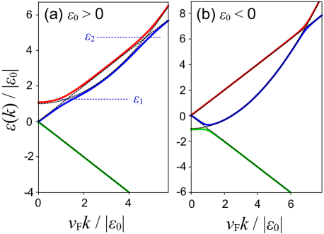
Figure 2: Band structure of the minimal hybridized model defined by Eqs. (53) and (54), for the energy offset (a) $\epsilon_{0}>0$ and (b) $\epsilon_{0}<0$. The parameters are taken as $m=3|\epsilon_{0}|$ and $h=0.2|\epsilon_{0}|$. The dashed lines show the bands without the hybridization $h$. $\epsilon_{1}$ and $\epsilon_{2}$ in (a) are the energies of the band crossing points in the absence of hybridization, which we shall use in later calculations.

Since this model Hamiltonian keeps the right-handed and left-handed components in the Dirac sector equivalent, it yields three bands, each of which is twofold degenerate and spherically symmetric around $\boldsymbol{k}=0$. Here we note that $H(\boldsymbol{k})$ commutes with the operator $\boldsymbol{e}_{k}\cdot\boldsymbol{\sigma}$, corresponding to the helicity of a particle. Therefore, $H(\boldsymbol{k})$ can be separated into two helicity subspaces characterized by the eigenvalue $\eta=\pm$, with the $3\times 3$-matrix

$$H_{\eta}(k)=\begin{pmatrix}\eta v_{\mathrm{F}}k&0&h\\ 0&-\eta v_{\mathrm{F}}k&h\\ h&h&\frac{k^{2}}{2m}+\epsilon_{0}\end{pmatrix}$$ (56)

for each subspace. The typical band structure based on this Hamiltonian is shown by Fig. 2. In the present model, the quadratic dispersion from the nonrelativistic sector coexists with the linear dispersion from the Dirac sector. Therefore, if the energy offset $\epsilon_{0}$ is positive, as shown in Fig. 2(a), the nonrelativistic band intersects the particle (electron) branch of the Dirac band twice, whose energy levels are labeled as $\epsilon_{1}$ and $\epsilon_{2}$ in the following discussions. At these points, the bands develop anticrossing with the amplitude $h$. If $\epsilon_{0}$ is negative, as shown in Fig. 2(b), the nonrelativistic band intersects the antiparticle (hole) and particle branches of the Dirac band once for each, yielding a gap at the crossing point with the antiparticle branch. In the present calculation, we take $\epsilon_{0}$ positive, and investigate the behavior of the SO crossed susceptibility mainly around the hybridization points $\epsilon_{1,2}$.

Our model defined here is composed of minimal number of degrees of freedom, in order to extract the common feature in the SO susceptibility caused solely by the presence or absence of the band hybridization. While realistic systems including relativistic fermions generally have richer internal degrees of freedom, such as orbital and sublattice degrees of freedom for electrons in solid states and color and flavor degrees of freedom for quarks in high-energy physics, dependence on such detailed internal structures for each system is beyond our interest in this article.

IV.2 Static and Dynamical suceptibilities

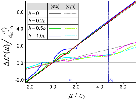
Figure 3: Behavior of the SO crossed susceptibility $\Delta\chi^{\mathrm{so}}(\mu)$, as functions of the Fermi energy $\mu$. The solid and dashed lines are the static and dynamical susceptibility, respectively, with the hybridization parameter $h$ varied as shown in the inset table. The vertical dashed lines $(\epsilon_{1,2})$ correspond to the band hybridization points, which are identical to those shown in Fig. 2(a). The parameters are taken as $\epsilon_{0}>0$ and $m=3\epsilon_{0}$.

With the model Hamiltonian defined in the previous subsection, we now evaluate the SO crossed susceptibility $\Delta\chi^{\mathrm{so}}(\mu)$ in both static and dynamical limits. We first consider the response of the net spin polarization, by taking the spin operator $\boldsymbol{\mathcal{S}}$ as a matrix $\mathrm{diag}(\boldsymbol{\sigma},\boldsymbol{\sigma},\boldsymbol{\sigma})/2$ acting on the 6-component field operator $\Psi$ in Eq. (55). Here we fix the band parameters $\epsilon_{0}>0$ and $m=3\epsilon_{0}$, and vary the band hybridization parameter $h$ and the Fermi energy $\mu$ to capture typical structures in $\Delta\chi^{\mathrm{so}}(\mu)$, arising from the band hybridization. We evaluate the formula obtained in Sec. II.3 numerically, based on the band eigenstates of the model Hamiltonian. The quantities with energy dimensions are rescaled by $\epsilon_{0}$ in the present calculations. Since the system is assumed to satisfy spherical symmetry, the susceptibility tensor possesses only the diagonal part $\Delta\chi^{\mathrm{so}}_{ij}(\mu)=\Delta\chi^{\mathrm{so}}(\mu)\delta_{ij}$, which we shall evaluate in the following discussion.

We first compare the static susceptibility $\Delta\chi^{\mathrm{so(sta)}}$ and the dynamical susceptibility $\Delta\chi^{\mathrm{so(dyn)}}$ under the band hybridization, with those estimated with the Dirac fermions without hybridization, which we call the “pure Dirac” case [Eqs. (40) and (41)]. The results are shown in Fig. 3 as functions of $\mu$. In the vicinity of the band hybridization points $\epsilon_{1,2}$, both the static susceptibility $\Delta\chi^{\mathrm{so(sta)}}$ and the dynamical susceptibility $\Delta\chi^{\mathrm{so(dyn)}}$ deviate from those in the pure Dirac case. They asymptotically reach the pure Dirac behavior at the energies away from $\epsilon_{1,2}$, since the hybridization effect on the band eigenstates is significant only around these points.

For the static susceptibility $\Delta\chi^{\mathrm{so(eq)}}(\mu)$, we find three nonanalytic cusps for each value of $h$. These cusps corresponds to the band edges, namely the minima and maxima of the bands under the hybridization. The origin of such a nonanalytic behavior can be traced back to the density of states, which becomes nonanalytic at each band edge. We can see that it comes from the intraband part of the magnetic-moment contribution $\chi_{ij}^{\mathrm{so(sta:}m)}$ given by Eq. (27), since it is accompanied with the factor $f^{\prime}(\epsilon_{a})$ that gives the density of states at zero-temperature limit. Nonanalyticity in the static susceptibility is also found for massive Dirac fermions [42], arising at the edges of the mass gap, which can also be attributed to the above mechanism.

In contrast, the dynamical susceptibility $\Delta\chi^{\mathrm{so(dyn)}}(\mu)$ is obtained as a smooth function in $\mu$, since it does not contain the intraband Fermi-surface contribution. Although it still contains the Fermi-surface effect $f^{\prime}(\epsilon_{a})$ in $\chi_{ij}^{\mathrm{so(dyn:}A)}$, the velocity $\boldsymbol{v}_{a}$ in the same term reaches zero at the band edge, canceling nonanalyticity from the density of states.

Aside from the nonanalyticity, we should note that the dynamical susceptibility $\Delta\chi^{\mathrm{so(dyn)}}(\mu)$ shows a relatively large deviation from the pure Dirac case around the hybridization points $\epsilon_{1,2}$. In particular, around $\epsilon_{2}$, the static susceptibility appears almost insensitive to the hybridization effect, whereas the dynamical suceptibility gets suppressed by the hybridization. This is because the dynamical susceptibility is dominated by the interband processes: the contribution from the interband processes, accompanied with the weight factor $F_{ab}=[f(\epsilon_{a}-\mu)-f(\epsilon_{b}-\mu)]/(\epsilon_{a}-\epsilon_{b})$, becomes significant at $\boldsymbol{k}$ around the hybridization point, as the two bands $\epsilon_{a}$ and $\epsilon_{b}$ get close to one another. As a result, the dynamical SO crossed susceptibility acquires a large modification from the band hybridization, in comparison with the static susceptibility.

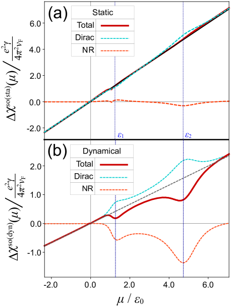
Figure 4: The SO crossed susceptibilities separated into the Dirac sector $\chi^{\mathrm{so}}_{\mathrm{Dirac}}$ and the nonrelativistic (NR) sector $\chi^{\mathrm{so}}_{\mathrm{NR}}$, and their sum (Total, $\chi^{\mathrm{so}}$). Panel (a) shows the static susceptibilities, while Panel (b) shows the dynamical susceptibilities. Both results are obtained with the offset of the NR band $\epsilon_{0}>0$, the effective mass for the NR band $m=3\epsilon_{0}$, and the hybridization parameter $h=0.2\epsilon_{0}$.

IV.3 Response of Dirac and nonrelativistic sectors

In order to understand the hybridization-induced modification in $\chi^{\mathrm{so}}(\mu)$ in more detail, we separate it into the contributions from the Dirac and nonrelativistic sectors. The spin magnetization for the Dirac sector $\boldsymbol{M}^{\mathrm{s}}_{\mathrm{Dirac}}$ and that for the nonrelativistic sector $\boldsymbol{M}^{\mathrm{s}}_{\mathrm{NR}}$ can be evaluated separately, with the spin operators

$$\boldsymbol{\mathcal{S}}_{\mathrm{Dirac}}=\frac{1}{2}\begin{pmatrix}\boldsymbol{\sigma}&0&0\\ 0&\boldsymbol{\sigma}&0\\ 0&0&0\end{pmatrix},\quad\boldsymbol{\mathcal{S}}_{\mathrm{NR}}=\frac{1}{2}\begin{pmatrix}0&0&0\\ 0&0&0\\ 0&0&\boldsymbol{\sigma}\end{pmatrix}.$$ (57)

As the response functions of these sector-resolved spin magnetizations to the orbital magnetic field $\boldsymbol{B}^{\mathrm{o}}$, we define the SO crossed susceptibilities for the Dirac and nonrelativistic sectors,

$$M^{\mathrm{s}}_{\mathrm{Dirac},i}=-\gamma\langle S_{\mathrm{Dirac},i}\rangle \equiv\chi^{\mathrm{so}}_{\mathrm{Dirac},ij}B^{\mathrm{o}}_{j}$$ (58)

$$M^{\mathrm{s}}_{\mathrm{NR},i}=-\gamma\langle S_{\mathrm{NR},i}\rangle \equiv\chi^{\mathrm{so}}_{\mathrm{NR},ij}B^{\mathrm{o}}_{j},$$ (59)

which are obtained by using $\boldsymbol{\mathcal{S}}_{\mathrm{Dirac}}$ and $\boldsymbol{\mathcal{S}}_{\mathrm{NR}}$ instead of $\boldsymbol{\mathcal{S}}$ in the formulas shown in Sec. II.3.

Based on the above definition, the sector-resolved susceptibilities as functions of the Fermi energy $\mu$ are obtained as shown in Fig. 4, (a) in the static limit and (b) in the dynamical limit. We here emphasize that $\chi^{\mathrm{so}}_{\mathrm{NR}}$ becomes nonzero around the hybridization points $\epsilon_{1,2}$ both in the static and dynamical limits, among which the effect in the dynamical limit appears rather significant. This indicates that the nonrelativistic sector shows a finite spin polarization in response to the orbital magnetic field, even though the nonrelativistic fermions are originally not subject to SOC.

Let us here give a qualitative discussion about the mechanism how the dynamical susceptibility is strongly influenced by the band hybridization, by using a perturbation theory with a simple quantum mechanics. What we need to evaluate is the spin magnetic moment of the hybridized states around the hybridization points. Since the orbital magnetic moment $\boldsymbol{m}_{aa}(\boldsymbol{k})$ of a massless Dirac (or Weyl) fermion is parallel to its spin magnetic moment $\boldsymbol{\mu}_{aa}(\boldsymbol{k})=-\gamma\boldsymbol{\mathcal{S}}_{aa}(\boldsymbol{k})$, as seen from Eqs. (36) and (39), here we substitute the orbital magnetic field with an effective spin magnetic field acting selectively on the Dirac sector, coupled to the spins as $\delta\mathcal{H}_{\mathrm{eff}}=\gamma\boldsymbol{B}^{\mathrm{s}}_{\mathrm{Dirac}}\cdot\boldsymbol{S}_{\mathrm{Dirac}}$. Note that this substitution of effective field is valid in describing only the direction of the induced spin polarization, not its magnitude including parameter dependences. We then take into account the hybridization between the Dirac and nonrelativistic sectors, and consider the response of spin magnetic moments to this effective magnetic field. For the sake of clarity, we take the direction of $\boldsymbol{B}^{\mathrm{s}}_{\mathrm{Dirac}}$ as $z$-axis, which yields $\delta\mathcal{H}_{\mathrm{eff}}=\gamma B^{\mathrm{s}}_{\mathrm{Dirac}}S^{z}_{\mathrm{Dirac}}$, and focus on the magnetic moments in this direction, as we are here interested in the responses in spatially isotropic systems.

At the momentum $\boldsymbol{k}_{c}$ where the Dirac and nonrelativistic bands cross each other, two states $|u_{\mathrm{Dirac}}(\boldsymbol{k}_{c})\rangle$ and $|u_{\mathrm{NR}}(\boldsymbol{k}_{c})\rangle$ get hybridized. The hybridized states are given as linear combinations of the two states,

$$|u_{\pm}\rangle =\tfrac{1}{\sqrt{2}}\left[|u_{\mathrm{Dirac}}\rangle\pm|u_{\mathrm{NR}}\rangle\right],$$ (60)

where the eigenenergies $\epsilon_{\pm}$ satisfy $\epsilon_{+}-\epsilon_{-}=2h$. If the hybridization does not mix spins, as we have assumed in the present model, $|u_{\mathrm{Dirac}}\rangle$ and $|u_{\mathrm{NR}}\rangle$ participating to the hybridization have the same spin polarizations. If the Fermi level $\mu$ lies between $\epsilon_{+}$ and $\epsilon_{-}$, only the occupied state $|u_{-}\rangle$ contributes to the spin polarization. Therefore, we see here how the spin magnetic moment of the state $|u_{-}\rangle$ gets perturbed by the effective magnetic field $\boldsymbol{B}^{\mathrm{s}}_{\mathrm{Dirac}}$.

When the effective magnetic field $\boldsymbol{B}^{\mathrm{s}}_{\mathrm{Dirac}}$ is applied, the state $|u_{-}\rangle$ is perturbed by $\delta\mathcal{H}_{\mathrm{eff}}$,

$$|\delta u_{-}\rangle =|u_{+}\rangle\frac{\langle u_{+}|\delta\mathcal{H}_{\mathrm{eff}}|u_{-}\rangle}{\epsilon_{-}-\epsilon_{+}}=-\frac{\gamma B^{\mathrm{s}}_{\mathrm{Dirac}}}{2h}|u_{+}\rangle\langle u_{+}|S^{z}_{\mathrm{Dirac}}|u_{-}\rangle$$ (61)

at first order in $\boldsymbol{B}^{\mathrm{s}}_{\mathrm{Dirac}}$. By this perturbation, the spin magnetic moments of $|u_{-}\rangle$ projected onto the Dirac and nonrelativistic sectors, which we denote as $\boldsymbol{\mu}_{\Gamma}=-\gamma\langle u_{-}|\boldsymbol{S}_{\Gamma}|u_{-}\rangle\ (\Gamma=\mathrm{Dirac},\mathrm{NR})$, get modified as

$$\delta\mu^{z}_{\Gamma} =-\gamma\delta\langle u_{-}|S^{z}_{\Gamma}|u_{-}\rangle=-2\gamma\mathrm{Re}\langle\delta u_{-}|S^{z}_{\Gamma}|u_{-}\rangle$$

$$=\frac{\gamma^{2}B^{\mathrm{s}}_{\mathrm{Dirac}}}{h}\mathrm{Re}\left[\langle u_{+}|S^{z}_{\Gamma}|u_{-}\rangle\langle u_{-}|S^{z}_{\mathrm{Dirac}}|u_{+}\rangle\right].$$ (62)

For the Dirac sector, the modification

$$\delta\mu^{z}_{\mathrm{Dirac}} =\frac{\gamma^{2}B^{\mathrm{s}}_{\mathrm{Dirac}}}{h}|\langle u_{+}|S^{z}_{\mathrm{Dirac}}|u_{-}\rangle|^{2}$$ (63)

is parallel to $B^{\mathrm{s}}_{\mathrm{Dirac}}$, from which we can qualitatively understand the enhancement of the SO response in the Dirac sector. We note that this mechanism is similar to the Van Vleck paramagnetism, where the paramagnetic susceptibility is enhanced by the interband effect that is allowed by SOC [58]. On the other hand, for $\delta\mu^{z}_{\mathrm{NR}}$, the matrix elements in Eq. (62) become

$$\langle u_{+}|S_{\mathrm{NR}}^{z}|u_{-}\rangle =-\tfrac{1}{2}\langle u_{\mathrm{NR}}|S_{\mathrm{NR}}^{z}|u_{\mathrm{NR}}\rangle$$ (64)

$$\langle u_{-}|S_{\mathrm{Dirac}}^{z}|u_{+}\rangle =\tfrac{1}{2}\langle u_{\mathrm{Dirac}}|S_{\mathrm{Dirac}}^{z}|u_{\mathrm{Dirac}}\rangle,$$ (65)

which yields

$$\delta\mu^{z}_{\mathrm{NR}} =-\frac{\gamma^{2}B^{\mathrm{s}}_{\mathrm{Dirac}}}{4h}\langle u_{\mathrm{NR}}|S_{\mathrm{NR}}^{z}|u_{\mathrm{NR}}\rangle\langle u_{\mathrm{Dirac}}|S_{\mathrm{Dirac}}^{z}|u_{\mathrm{Dirac}}\rangle.$$ (66)

Since we have assumed that $|u_{\mathrm{Dirac}}\rangle$ and $|u_{\mathrm{NR}}\rangle$ have the same spin direction, $\langle u_{\mathrm{Dirac}}|S_{\mathrm{Dirac}}^{z}|u_{\mathrm{Dirac}}\rangle$ and $\langle u_{\mathrm{NR}}|S_{\mathrm{NR}}^{i}|u_{\mathrm{NR}}\rangle$ have the same signs, which is the case with the present model Hamiltonian in Eq. (54). Therefore, the product of the two matrix elements in Eq. (62) becomes negative, yielding $\delta\mu^{z}_{\mathrm{NR}}$ antiparallel to $B^{\mathrm{s}}_{\mathrm{Dirac}}$. This discussion provides qualitative interpretation about the negative SO response induced in the nonrelativistic sector seen in Fig. 4(b), which is due to the structure of the hybridized states.

Our calculation results of the SO crossed susceptibility using the minimal model in Eqs. (53) and (54) are well described by the above discussion with a simple quantum mechanics. This discussion is valid no matter what kind of internal degrees of freedom is present, such as orbital, sublattice, flavor, or color. Therefore, we can understand that the modifications in the SO susceptibilities found in our calculation are not the artifact from the minimal model employed here. It is the common feature available in any relativistic fermion systems hybridized with nonrelativistic fermion degrees of freedom, as long as the hybridization mixes two states with the same spin direction.

V Implication on experiments

Finally, we give some discussions about the implications of our findings on experiments. In order to realize our idea in experimental measurements, we first need to note the hierarchy of energy (time) scales, among the relaxation rate (inverse relaxation time) $\tau^{-1}$, the hybridization energy $h$, and the frequency of the external magnetic field $\Omega$. As mentioned in Sec. II.2, the static limit is valid for $\Omega<\tau^{-1}<h$, and the dynamical limit applies to the case $\tau^{-1}<\Omega<h$. For example, the transport calculations in graphene with charged impurities give the relaxation time around $\tau\sim 1\mathrm{ps}$, corresponding to the frequency $\tau^{-1}\sim 1\mathrm{THz}$ and the energy $4\mathrm{meV}$ [105]. This can be regarded as the typical scale of relaxation for Dirac electrons at low carrier density, with the Fermi velocity comparable to that of graphene ($v_{\mathrm{F}}=3\times 10^{6}\mathrm{m/s}$). With this relaxation timescale, transition between the static and dynamical behaviors in the susceptibility can be achieved by varying the frequency of the external magnetic field around the terahertz regime. The hybridization energy $h$ should be larger than $\tau^{-1}$, so that the spectral broadening by the imaginary part of the fermion self energy may not obscure the band splitting of $h$ arising from the hybridization effect.

V.1 Solid states

For electrons in solid states, the response to a magnetic field measured in experiments contains both the response to the orbital magnetic field discussed throughout this article and the response to the spin magnetic field via the Zeeman effect. In order to extract the orbital effect, one may excite the orbital degrees of freedom selectively by a circularly polarized light, and observe the magnetic circular dichroism, namely the difference in the light absorption depending on the polarization of the light [106]. Another way to identify the orbital effect is to subtract the spin effect from the full response to the magnetic field. In order to extract the spin effect, one may rely on the exchange coupling between the spins of localized electrons in magnetic elements and the spins of itinerant electrons, which takes the same form with the Zeeman coupling. By introducing magnetic dopants in bulk sample, or the magnetic proximity effect in thin-film geometry attached with a magnetic material, we can mimic the spin magnetic field for the itinerant electrons, from which we may extract the response to the spin magnetic field.

Aside from the total spin polarization, we are also interested in the spin polarization separated into the Dirac and nonrelativistic sectors, as discussed in Sec. IV.3. In order to distinguish the spin polarization by the sectors, the nuclear magnetic resonance (NMR) spectroscopy will be helpful in some materials [107]. We may rely on the Knight shift in the NMR spectrum, which arises from the hyperfine coupling bewteen the electron spin and the nuclear magnetic moment [108]. The Knight shift provides information about the electron spin polarization belonging to each constituent element in the compound. Therefore, if the Dirac and nonrelativistic bands in the material come from different elements, such as in a Dirac semimetal with impurity dopants, the Knight shift may provide information about the sector-resolved spin polarization mentioned in our discussion.

V.2 Quark matter

Our discussion can also be applied to quark matter. In particular, we may consider mixture of heavy quarks, corresponding to the flavor $c$ and sometimes $b$, and light quarks $u$, $d$, and $s$. Light quarks, having Dirac masses relatively smaller than heavy quarks, can be treated as Dirac fermions, while heavy quarks behave as nonrelativistic fermions at low momentum. Throughout a relativistic heavy-ion collision process, the generated quark matter will be subject to a magnetic field, if the collision of two heavy nuclei is noncentral [88, 109, 110, 111, 112]. In a manner similar to the CME and the CSE proposed in quark matter, this magnetic field will give rise to the spin polarization of both the light and heavy quarks. Since light quarks are described as relativistic Dirac fermions, the magnetic field couples to them only via the vector potential. While heavy quarks behave as nonrelativistic fermions, the Zeeman effect on them is almost negligible due to their large Dirac masses. Therefore, the effect of the magnetic field on the spin polarization of quarks can be dominantly described by the SO crossed susceptibility $\chi^{\mathrm{so}}$.

Hybridization of light and heavy quarks is possible, if heavy quarks are dilute enough in comparison with light quarks. Heavy quarks form bound states with light quarks by the strong interaction, which is proposed as the QCD Kondo effect [21, 22, 23, 24, 25, 26, 27, 28, 29, 30, 31, 32, 33, 34, 35, 36, 37, 38, 39, 40]. Under such a hybridization, our analysis on the SO susceptibility implies that heavy quarks, corresponding to the nonrelativistic sector in our analysis, develop spin polarization in response to a magnetic field, although the Zeeman coupling for heavy quarks is weak. While the spin polarization of heavy quarks cannot be measured directly, it may be captured as spin polarization of heavy hadrons including heavy quarks ($c$ or $b$) after hadronization, where the quarks are cooled down and confined in hadrons. In the hadronization process, spin polarization of heavy quark can be transferred to spin polarization of a $\Lambda_{c}$ or $\Lambda_{b}$ baryon. Therefore, measurement of the spin polarization of the $\Lambda_{c}$ or $\Lambda_{b}$ baryon is one of the promising ways to observe the hybridization induced by the QCD Kondo effect which is not experimentally verified so far. In order to understand such an effect in quark matter precisely, one needs to determine the microscopic structure of interaction and parameters specific to the system, which is left for further analysis [113].

VI Conclusion

In the present article, we have focused on the SO crossed susceptibility, namely the response function of the spin magnetization $\boldsymbol{M}^{\mathrm{s}}$ composed of the spin polarization of fermions, to the orbital magnetic field $\boldsymbol{B}^{\mathrm{o}}$ described by the U(1) vector potential. The SO crossed susceptibility quantifies the relativistic effect acting on fermions, since it arises as a consequence of SOC, which is the relativistic effect. The idea of SO susceptibility is applicable to any kind of fermion system, not limited to solid states but also to quark matter.

One of the main issues discussed in this work is the comparison of the SO crossed susceptibilities in two limits, namely the static and dynamical limits. While the behavior of the SO crossed susceptibility in the static limit, induced by a slowly introduced magnetic field keeping the equilibrium, is broadly discussed in the context of topological materials, its dynamical-limit behavior, under an abruptly introduced magnetic field that drives the distribution out of equilibrium, is discussed systematically for the first time.

As a result of our analysis, we have found that the difference between the static and dynamical SO susceptibilities becomes significant in the presence of band hybridization. We have seen this tendency by using the hybridized model of Dirac fermions obeying spin-momentum locking and nonrelativistic fermions free from SOC. In the dynamical limit, the SO susceptibility gets strongly modified by the hybridization, and the spins of the nonrelativistic fermions also respond to the orbital magnetic field, even though they are not originally subject to SOC. These modification effects can be understood as the outcome of interband perturbation effect allowed by the band hybridization, which is in a mechanism similar to the Van Vleck paramagnetism.

The framework of our discussion applies at various energy scales, such as electrons in solids and quark matter after heavy-ion collision in accelerators. In the present article, we have taken a simple model with minimal number of degrees of freedom, with which we are successful in extracting a common feature in the SO susceptibility triggered by the hybridization of relativistic and nonrelativistic degrees of freedom. Of course, in realistic systems, there may be more diverse internal degrees of freedom, depending on the atomic orbitals and crystalline symmetries for electrons in solid states and color and flavor degrees of freedom for quarks in high-energy physics. Detailed treatment of the crossed response phenomena, based on the microscopic model for each setup, will be left for future analysis.

Appendix A Orbital and spin magnetizations

In this part of the appendix, we review how a magnetic field couples to the orbital and spin degrees of freedom, and distinguish the SO crossed susceptibility from the other types of magnetic susceptibilities.

For relativistic fermions under Lorentz symmetry, their coupling to a magnetic field $\boldsymbol{B}$ is given in terms of covariant derivative, with the vector potential $\boldsymbol{A}(\boldsymbol{r})$ corresponding to the magnetic field $\boldsymbol{B}=\boldsymbol{\nabla}\times\boldsymbol{A}$. On the other hand, for nonrelativistic fermions, such as electrons trapped in crystals (including electrons in topological semimetals with the Dirac- or Weyl-type dispersion at low energy), their coupling to a magnetic field is classified into (a) the orbital effect and (b) the spin effect, which can be derived by downfolding the relativistic theory to the nonrelativistic limit.

(a) The orbital effect is given in terms of covariant derivative, which is similar to the gauge coupling in the relativistic theory. If the dynamics of fermions is described by the continuum Hamiltonian

$$\mathcal{H}_{0} =\int d\boldsymbol{r}\ \psi^{\dagger}(\boldsymbol{r})H(\boldsymbol{p})\psi(\boldsymbol{r}),$$ (67)

where $\psi(\boldsymbol{r})$ is the (multi-component) field operator of the fermions and $H(\boldsymbol{p})$ is defined by substituting the momentum operator $\boldsymbol{p}=-i\boldsymbol{\nabla}$ to the momentum-space Hamiltonian $H(\boldsymbol{k})$, the vector potential shifts the Hamiltonian as

$$\mathcal{H}=\int d\boldsymbol{r}\ \psi^{\dagger}(\boldsymbol{r})H(\boldsymbol{p}-e\boldsymbol{A}(\boldsymbol{r}))\psi(\boldsymbol{r}),$$ (68)

with $-e$ the electric charge of the fermion. Therefore, the perturbation by the magnetic field is extracted as

$$\delta\mathcal{H}^{\mathrm{o}} =-\frac{e}{2}\int d\boldsymbol{r}\ \psi^{\dagger}(\boldsymbol{r})\{\boldsymbol{v}(\boldsymbol{p}),\boldsymbol{A}(\boldsymbol{r})\}\psi(\boldsymbol{r}),$$ (69)

with the velocity operator $\boldsymbol{v}(\boldsymbol{p})=\partial H(\boldsymbol{p})/\partial\boldsymbol{p}$.

(b) The spin effect is the so-called Zeeman splitting, namely the coupling between the spin angular momentum and the magnetic field. If the spin density operator of the fermions is given as $\boldsymbol{S}=\psi^{\dagger}\boldsymbol{\mathcal{S}}\psi$, with $\boldsymbol{\mathcal{S}}$ the matrix acting on the components of the field operator, the spin effect of the magnetic field is given in terms of the Zeeman term,

$$\delta\mathcal{H}^{\mathrm{s}} =\gamma\int d\boldsymbol{r}\ \boldsymbol{B}\cdot\boldsymbol{S}=\gamma\int d\boldsymbol{r}\ \psi^{\dagger}(\boldsymbol{B}\cdot\boldsymbol{\mathcal{S}})\psi.$$ (70)

Here $\gamma=g\mu_{B}$ is the parameter called gyromagnetic ratio, with $\mu_{B}$ the Bohr magneton and $g$ is the $g$-factor for the fermions. Note that $g$ may depend on internal degrees of freedom, such as the species of fermions, the atomic orbitals that the electrons in the crystal belong to, etc., whereas we here neglect such detailed structures.

Although the origins of the above two effects are the same magnetic field $\boldsymbol{B}$, one may formally distinguish them by using different labels for the magnetic field, $\boldsymbol{B}^{\mathrm{o}}$ and $\boldsymbol{B}^{\mathrm{s}}$. Under the orbital and spin magnetic fields, the partition function $Z[\boldsymbol{B}^{\mathrm{o}},\boldsymbol{B}^{\mathrm{s}}]$ is given from the perturbed Hamiltonian $\mathcal{H}_{0}+\delta\mathcal{H}^{\mathrm{o}}[\boldsymbol{B}^{\mathrm{o}}]+\delta\mathcal{H}^{\mathrm{s}}[\boldsymbol{B}^{\mathrm{s}}]$ by tracing out the fermionic degrees of freedom $(\psi^{\dagger},\psi)$. From this partition function, the magnetization can also be defined separately for the orbital and spin sectors, as thermodynamic variables conjugate to $\boldsymbol{B}^{\mathrm{o}}$ and $\boldsymbol{B}^{\mathrm{s}}$:

$$\boldsymbol{M}^{\mathrm{o}}=-\frac{\delta\ln Z}{\delta\boldsymbol{B}^{\mathrm{o}}}\biggr{|}_{\boldsymbol{B}^{\mathrm{o}}=\boldsymbol{B}^{\mathrm{s}}=0},\ \boldsymbol{M}^{\mathrm{s}}=-\frac{\delta\ln Z}{\delta\boldsymbol{B}^{\mathrm{s}}}\biggr{|}_{\boldsymbol{B}^{\mathrm{o}}=\boldsymbol{B}^{\mathrm{s}}=0}.$$

The spin magnetization $\boldsymbol{M}^{\mathrm{s}}$ is composed of the spins of the fermions, related to the expectation value of spin polarization $\langle\boldsymbol{S}\rangle$ as

$$\boldsymbol{M}^{\mathrm{s}}=-\gamma\langle\boldsymbol{S}\rangle=-\gamma\langle\psi^{\dagger}\boldsymbol{\mathcal{S}}\psi\rangle.$$ (71)

On the other hand, the orbital magnetization $\boldsymbol{M}^{\mathrm{o}}$ comes from the orbital angular momenta of the fermions, corresponding to the circulating electric current carried by the fermions. Since the position operator $\boldsymbol{r}$ is ill-defined in unbounded systems, the momentum-space formalism of orbital magnetization $\boldsymbol{M}^{\mathrm{o}}$ cannot be given so simply as the spin magnetization $\boldsymbol{M}^{\mathrm{s}}$ [see Eq. (30)].

The magnetic susceptibility $\chi_{ij}$ is defined as the tensor characterizing the response of magnetization $\delta M_{i}$ to the magnetic field $B_{j}$. As the magnetic field and the magnetization are separated into the orbital and spin parts defined above, the magnetic susceptibility can be separated into the four parts:

[Spin-spin] $$\delta M^{\mathrm{s}}_{i}={\chi}^{\mathrm{ss}}_{ij}B^{\mathrm{s}}_{j},$$ (72)

[Spin-orbital] $$\delta M^{\mathrm{s}}_{i}={\chi}^{\mathrm{so}}_{ij}B^{\mathrm{o}}_{j},$$ (73)

[Orbital-spin] $$\delta M^{\mathrm{o}}_{i}={\chi}^{\mathrm{os}}_{ij}B^{\mathrm{s}}_{j},$$ (74)

[Orbital-orbital] $$\delta M^{\mathrm{o}}_{i}={\chi}^{\mathrm{oo}}_{ij}B^{\mathrm{o}}_{j}.$$ (75)

The spin-spin response is known as the Pauli paramagnetism, namely, the spin polarization induced by the Zeeman splitting, and the orbital-orbital part often gives rise to the Landau diamagnetism, due to the orbital magnetic moment of the quantum Hall states under the Landau quantization. The spin-orbital crossed parts $\chi^{\mathrm{so}}$ and $\chi^{\mathrm{os}}$ are not classified with either of them, which require the correlation between the spin and orbital degrees of freedom.

The above four susceptibilities are given in terms of the partition function $Z[\boldsymbol{B}^{\mathrm{o}},\boldsymbol{B}^{\mathrm{s}}]$,

$$\chi^{\mathrm{ss}}_{ij}=-\frac{\delta^{2}\ln Z}{\delta B^{\mathrm{s}}_{i}\delta B^{\mathrm{s}}_{j}}, \quad\chi^{\mathrm{so}}_{ij}=-\frac{\delta^{2}\ln Z}{\delta B^{\mathrm{s}}_{i}\delta B^{\mathrm{o}}_{j}},$$ (76)

$$\chi^{\mathrm{os}}_{ij}=-\frac{\delta^{2}\ln Z}{\delta B^{\mathrm{o}}_{i}\delta B^{\mathrm{s}}_{j}}, \quad\chi^{\mathrm{oo}}_{ij}=-\frac{\delta^{2}\ln Z}{\delta B^{\mathrm{o}}_{i}\delta B^{\mathrm{o}}_{j}}.$$ (77)

The spin-orbital crossed parts $\chi^{\mathrm{so}}$ and $\chi^{\mathrm{os}}$ satisfy the relation

$$\chi^{\mathrm{so}}_{ij}=\chi^{\mathrm{os}}_{ji},$$ (78)

which is the outcome of the Onsager’s reciprocity theorem [80].

Although magnetic field and magnetization in the relativistic regime cannot be separated into the orbital and spin parts, the idea of the SO crossed susceptibility $\chi^{\mathrm{so}}$ still applies. The spin magnetization can be defined from the spin polarization, $\boldsymbol{M}^{\mathrm{s}}=-\gamma\langle\boldsymbol{S}\rangle$, and the magnetic field $\boldsymbol{B}$ couples to the particles only via the vector potential. Therefore, in the relativistic regime, the response of the spin magnetization to the magnetic field is described in terms of $\chi^{\mathrm{so}}$ defined above.

Appendix B Detailed derivation process of the SO susceptibility tensor

In this appendix, we show details of the derivation process toward the formula for $\chi^{\mathrm{so}}$, whose final form is given in Sec. II.3.

B.1 Perturbation by vector potential

The starting point is the perturbation by the coupling to the vector potential $\boldsymbol{A}$. With the perturbation Hamiltonian $\delta H^{\mathrm{o}}$ given by Eq. (10), the linear perturbation of the Green’s function becomes

$$\delta G(\boldsymbol{k},i\omega_{n};\boldsymbol{k}^{\prime},i\omega_{n}^{\prime})$$ (79)

$$=G(\boldsymbol{k},i\omega_{n})\delta H^{\mathrm{o}}(\boldsymbol{k},i\omega_{n};\boldsymbol{k}^{\prime},i\omega_{n}^{\prime})G(\boldsymbol{k}^{\prime},i\omega_{n}^{\prime}),$$

which is nondiagonal in momentum and Matsubara frequency. Using this perturbation of Green’s function, the expectation value of the spin polarization $\langle\boldsymbol{S}(\boldsymbol{q},i\bar{\omega}_{m})\rangle$ induced by the vector potential $\boldsymbol{A}(\boldsymbol{q},i\bar{\omega}_{m})$ reads

$$\langle S_{i}(\boldsymbol{q},i\bar{\omega}_{m})\rangle$$

$$=\int d\boldsymbol{r}d\tau\ e^{i\boldsymbol{q}\cdot\boldsymbol{r}+i\bar{\omega}_{m}\tau}\langle S_{i}(\boldsymbol{r},\tau)\rangle$$ (80)

$$=\int d\boldsymbol{r}d\tau\ e^{i\boldsymbol{q}\cdot\boldsymbol{r}+i\bar{\omega}_{m}\tau}\langle\psi^{\dagger}(\boldsymbol{r},\tau)\mathcal{S}_{i}\psi(\boldsymbol{r},\tau)\rangle$$ (81)

$$=\int\frac{d\boldsymbol{r}d\tau}{(\beta V)^{2}}\sum_{i\omega_{n},i\omega^{\prime}_{n}}\sum_{\boldsymbol{k},\boldsymbol{k}^{\prime}}e^{i(\boldsymbol{q}+\boldsymbol{k}^{\prime}-\boldsymbol{k})\cdot\boldsymbol{r}+i(\bar{\omega}_{m}+\omega^{\prime}_{n}-\omega_{n})\tau}$$

$$\hskip 99.58464pt\times\langle\psi^{\dagger}(\boldsymbol{k}^{\prime},i\omega^{\prime}_{n})\mathcal{S}_{i}\psi(\boldsymbol{k},i\omega_{n})\rangle$$ (82)

$$=\frac{1}{\beta V}\sum_{i\omega_{n},\boldsymbol{k}}\left\langle\psi^{\dagger}(\boldsymbol{k}-\boldsymbol{q},i\omega_{n}-i\bar{\omega}_{m})\mathcal{S}_{i}\psi(\boldsymbol{k},i\omega_{n})\right\rangle$$ (83)

$$=\frac{-1}{\beta V}\sum_{i\omega_{n},\boldsymbol{k}}\mathrm{Tr}\left[\mathcal{S}_{i}\delta G(\boldsymbol{k},i\omega_{n};\boldsymbol{k}-\boldsymbol{q},i\omega_{n}-i\bar{\omega}_{m})\right]$$ (84)

$$=\frac{-1}{\beta V}\sum_{i\omega_{n},\boldsymbol{k}}\mathrm{Tr}\bigl{[}\mathcal{S}_{i}G(\boldsymbol{k},i\omega_{n})\delta H(\boldsymbol{k},\boldsymbol{k}-\boldsymbol{q})$$ (85)

$$\quad\quad\quad\quad\quad\quad\quad\quad\times G(\boldsymbol{k}-\boldsymbol{q},i\omega_{n}-i\bar{\omega}_{m})\bigr{]}$$

$$=-\frac{eA_{l}(\boldsymbol{q},i\bar{\omega}_{m})}{2\beta V}\sum_{i\omega_{n},\boldsymbol{k}}\mathrm{Tr}\bigl{\{}\mathcal{S}_{i}G(\boldsymbol{k},i\omega_{n})$$ (86)

$$\quad\quad\quad\quad\times\left[v_{l}(\boldsymbol{k})+v_{l}(\boldsymbol{k}-\boldsymbol{q})\right]G(\boldsymbol{k}-\boldsymbol{q},i\omega_{n}-i\bar{\omega}_{m})\bigr{\}}$$

$$\equiv\Pi_{A_{l}}^{\mathcal{S}_{i}}(\boldsymbol{q},i\bar{\omega}_{m})A_{l}(\boldsymbol{q},i\bar{\omega}_{m}),$$ (87)

where $i\bar{\omega}_{m}=i\tfrac{2\pi}{\beta}m$ is the bosonic Matsubara frequency corresponding to the frequency of the vector potential. This form corresponds to Eq. (11). By the analytical continuation $i\bar{\omega}_{m}\rightarrow\Omega+i0$, we obtain the linear response to the vector potential,

$$\langle S_{i}(\boldsymbol{q},\Omega)\rangle =\Pi_{A_{l}}^{S_{i}}(\boldsymbol{q},\Omega)A_{l}(\boldsymbol{q},\Omega),$$ (88)

for finite momentum $\boldsymbol{q}$ and frequency $\Omega$.

B.2 Description with band eigenstates

We need to evaluate the response tensor $\Pi_{A_{l}}^{S_{i}}(\boldsymbol{q},\Omega)$ up to $O(\boldsymbol{q})$, to apply Eq. (16). By decomposing the Green’s function as

$$G(\boldsymbol{k},i\omega_{n}) =-\sum_{a}\frac{|u_{a}(\boldsymbol{k})\rangle\langle u_{a}(\boldsymbol{k})|}{i\omega_{n}^{+}-\epsilon_{a}(\boldsymbol{k})},$$ (89)

where $a$ denotes the band index satisfying

$$H(\boldsymbol{k})|u_{a}(\boldsymbol{k})\rangle=\epsilon_{a}(\boldsymbol{k})|u_{a}(\boldsymbol{k})\rangle$$ (90)

and $i\omega_{n}^{+}=i\omega_{n}+\mu$, the response tensor is given in terms of matrix elements as

$$\Pi_{A_{l}}^{S_{i}}(\boldsymbol{q},i\bar{\omega}_{m})$$

$$=\frac{-e}{2\beta V}\sum_{i\omega_{n},\boldsymbol{k}}\mathrm{Tr}\Bigl{\{}\mathcal{S}_{i}G(\boldsymbol{k},i\omega_{n})$$ (91)

$$\hskip 28.45274pt\times\left[v_{l}(\boldsymbol{k})+v_{l}(\boldsymbol{k}-\boldsymbol{q})\right]G(\boldsymbol{k}-\boldsymbol{q},i\omega_{n}-i\bar{\omega}_{m})\Bigr{\}}$$

$$=\frac{-e}{2\beta V}\sum_{i\omega_{n},\boldsymbol{k}}\sum_{ab}\frac{\langle u_{b}(\boldsymbol{k}-\boldsymbol{q})|\mathcal{S}_{i}|u_{a}(\boldsymbol{k})\rangle}{\left[i\omega_{n}^{+}-\epsilon_{a}(\boldsymbol{k})\right]\left[i\omega_{n}^{+}-i\bar{\omega}_{m}-\epsilon_{b}(\boldsymbol{k}-\boldsymbol{q})\right]}$$

$$\hskip 28.45274pt\times\langle u_{a}(\boldsymbol{k})|v_{l}(\boldsymbol{k})+v_{l}(\boldsymbol{k}-\boldsymbol{q})|u_{b}(\boldsymbol{k}-\boldsymbol{q})\rangle$$ (92)

$$\equiv\frac{-e}{\beta V}\sum_{i\omega_{n},\boldsymbol{k}}\sum_{ab}\frac{\mathcal{M}_{ab}^{il}(\boldsymbol{k},\boldsymbol{q})}{\left[i\omega_{n}^{+}-\epsilon_{a}(\boldsymbol{k})\right]\left[i\omega_{n}^{+}-i\bar{\omega}_{m}-\epsilon_{b}(\boldsymbol{k}-\boldsymbol{q})\right]}.$$ (93)

Here $\mathcal{M}_{ab}^{il}(\boldsymbol{k},\boldsymbol{q})$ defined in the last line corresponds to Eq. (13).

The Matsubara summation is evaluated as

$$\frac{1}{\beta}\sum_{i\omega_{n}}\frac{1}{\left[i\omega_{n}^{+}-\epsilon_{a}(\boldsymbol{k})\right]\left[i\omega_{n}^{+}-i\bar{\omega}_{m}-\epsilon_{b}(\boldsymbol{k}-\boldsymbol{q})\right]}$$

$$=\frac{f(\epsilon_{a}(\boldsymbol{k})-\mu)-f(\epsilon_{b}(\boldsymbol{k}-\boldsymbol{q})-\mu+i\bar{\omega}_{m})}{-i\bar{\omega}_{m}+\epsilon_{a}(\boldsymbol{k})-\epsilon_{b}(\boldsymbol{k}-\boldsymbol{q})}$$ (94)

$$=\frac{f(\epsilon_{a}(\boldsymbol{k})-\mu)-f(\epsilon_{b}(\boldsymbol{k}-\boldsymbol{q})-\mu)}{-i\bar{\omega}_{m}+\epsilon_{a}(\boldsymbol{k})-\epsilon_{b}(\boldsymbol{k}-\boldsymbol{q})}$$ (95)

$$\overset{i\bar{\omega}_{m}\rightarrow\Omega+i0}{\longrightarrow}\frac{f(\epsilon_{a}(\boldsymbol{k})-\mu)-f(\epsilon_{b}(\boldsymbol{k}-\boldsymbol{q})-\mu)}{\epsilon_{a}(\boldsymbol{k})-\epsilon_{b}(\boldsymbol{k}-\boldsymbol{q})-\Omega-i0}\equiv\mathcal{F}_{ab}(\boldsymbol{k},\boldsymbol{q},\Omega),$$

which corresponds to Eq. (14). We thus obtain Eq. (12),

$$\Pi^{S_{i}}_{A_{l}}(\boldsymbol{q},\Omega) =-\frac{e}{V}\sum_{\boldsymbol{k}}\sum_{ab}\mathcal{F}_{ab}(\boldsymbol{k},\boldsymbol{q},\Omega)\mathcal{M}_{ab}^{il}(\boldsymbol{k},\boldsymbol{q}).$$ (96)

B.3 Expansion by $\boldsymbol{q}$

We need to expand $\Pi_{A_{j}}^{\mathcal{O}}(\boldsymbol{q},\Omega)$ up to $O(\boldsymbol{q})$ to derive the response to the magnetic field. By expanding $\mathcal{F}_{ab}(\boldsymbol{k},\boldsymbol{q},\Omega)$ and $\mathcal{M}_{ab}^{il}(\boldsymbol{k},\boldsymbol{q})$ as

$$\mathcal{F}_{ab}(\boldsymbol{k},\boldsymbol{q},\Omega) =\mathcal{F}_{ab}^{(0)}(\boldsymbol{k},\Omega)-q_{h}\mathcal{F}_{ab}^{(1)h}(\boldsymbol{k},\Omega)+O(q^{2}),$$ (97)

$$\mathcal{M}_{ab}^{il}(\boldsymbol{k},\boldsymbol{q}) =\mathcal{M}_{ab}^{(0)il}(\boldsymbol{k})-q_{h}\mathcal{M}_{ab}^{(1)ilh}(\boldsymbol{k})+O(q^{2}),$$ (98)

$\chi^{\mathrm{so}}_{ij}(\boldsymbol{q}=0,\Omega)$ can be obtained from Eq. (16) as

$$\chi^{\mathrm{so}}_{ij}(\boldsymbol{q}=0,\Omega)=\frac{i}{2}\gamma\epsilon_{jlh}\frac{\partial\Pi^{S_{i}}_{A_{l}}(\boldsymbol{q},\Omega)}{\partial q_{h}}\biggr{|}_{\boldsymbol{q}=0}$$ (99)

$$\hskip 28.45274pt=-\frac{ie}{2V}\epsilon_{jlh}\sum_{\boldsymbol{k}}\sum_{ab}\left[\mathcal{F}_{ab}^{(1)h}\mathcal{M}_{ab}^{(0)il}+\mathcal{F}_{ab}^{(0)}\mathcal{M}_{ab}^{(1)ilh}\right].$$

The expansion of the matrix elements $\mathcal{M}_{ab}^{il}(\boldsymbol{k},\boldsymbol{k}-\boldsymbol{q})$ is given by

$$\mathcal{M}_{ab}^{(0)il} =\langle u_{a}|v_{l}|u_{b}\rangle\langle u_{b}|\mathcal{S}_{i}|u_{a}\rangle,$$ (100)

$$\mathcal{M}_{ab}^{(1)ilh} =\tfrac{1}{2}\langle u_{a}|\partial_{k_{h}}v_{l}|u_{b}\rangle\langle u_{b}|\mathcal{S}_{i}|u_{a}\rangle$$ (101)

$$\quad+\langle u_{a}|v_{l}|\partial_{k_{h}}u_{b}\rangle\langle u_{b}|\mathcal{S}_{i}|u_{a}\rangle$$

$$\quad+\langle u_{a}|v_{l}|u_{b}\rangle\langle\partial_{k_{h}}u_{b}|\mathcal{S}_{i}|u_{a}\rangle,$$

where the dependence on $\boldsymbol{k}$ is not explicitly written for simplicity. $v_{a}^{h}$ is the group velocity, defined by $v_{a}^{h}=\partial_{k_{h}}\epsilon_{a}$. Since the first term in $\mathcal{M}_{ab}^{(1)ilh}$ contains $\partial_{k_{h}}v_{l}=\partial_{k_{h}}\partial_{k_{l}}H(\boldsymbol{k})$, which is symmetric in $h\leftrightarrow l$, it does not contribute to $\chi^{\mathrm{so}}_{ij}(\boldsymbol{q},\Omega)$ after the antisymmetrization by $\epsilon_{jlh}$.

On evaluating the weight factor $\mathcal{F}_{ab}(\boldsymbol{k},\boldsymbol{q},\Omega)$, we should be careful about the difference between the static and dynamical limits, which comes from the absence or presence of the frequency $\Omega$ in the denominator.

• For the interband process $\epsilon_{a}\neq\epsilon_{b}$, the numerator and the denominator remain finite in the limit $\boldsymbol{q}\rightarrow 0$ and $\Omega\rightarrow 0$ irrespective of the order of taking these two limits, and hence the $\boldsymbol{q}$-expansion of $\mathcal{F}_{ab}(\boldsymbol{k},\boldsymbol{q},\Omega\rightarrow 0)$ is straightforwardly given as

  $$\mathcal{F}_{ab}^{(0)} =\frac{f_{a}-f_{b}}{\epsilon_{a}-\epsilon_{b}},$$ (102)

  $$\mathcal{F}_{ab}^{(1)h} =v_{a}^{h}\left[\frac{f_{a}-f_{b}}{(\epsilon_{a}-\epsilon_{b})^{2}}-\frac{f^{\prime}_{a}}{\epsilon_{a}-\epsilon_{b}}\right],$$

  in both the static and dynamical limits.

• For the intraband process $\epsilon_{a}=\epsilon_{b}$, the denominator approaches zero in the limit $\boldsymbol{q}\rightarrow 0$ and $\Omega\rightarrow 0$, and hence we need to care about the order of taking these two limits. In the static limit, where the limit $\Omega=0$ is taken first, both the numerator and the denominator approach zero in the limit $\boldsymbol{q}\rightarrow 0$, yielding

  $$\mathcal{F}_{ab}(\boldsymbol{k},\boldsymbol{q},\Omega=0)|_{\epsilon_{a}=\epsilon_{b}}$$ (103)

  $$=\frac{f(\epsilon_{a}(\boldsymbol{k}))-f(\epsilon_{a}(\boldsymbol{k}-\boldsymbol{q}))}{\epsilon_{a}(\boldsymbol{k})-\epsilon_{a}(\boldsymbol{k}-\boldsymbol{q})}\overset{\boldsymbol{q}\rightarrow 0}{\longrightarrow}f^{\prime}(\epsilon_{a}(\boldsymbol{k}))=f^{\prime}_{a},$$

  which is of $O(q^{0})$. In the dynamical limit, where $\Omega$ is kept finite first, the denominator remains finite in the limit $\boldsymbol{q}\rightarrow 0$. Therefore, the $\boldsymbol{q}$-expansion becomes

  $$\mathcal{F}_{ab}(\boldsymbol{k},\boldsymbol{q},\Omega)|_{\epsilon_{a}=\epsilon_{b}}$$ (104)

  $$=\frac{f(\epsilon_{a}(\boldsymbol{k}))-f(\epsilon_{a}(\boldsymbol{k}-\boldsymbol{q}))}{\epsilon_{a}(\boldsymbol{k})-\epsilon_{a}(\boldsymbol{k}-\boldsymbol{q})-\Omega}=-\frac{q_{h}v_{a}^{h}f^{\prime}_{a}}{\Omega}+O(q^{2}),$$

  which is of $O(q^{1})$. Although it appears to diverge in the limit $\Omega\rightarrow 0$, it does not contribute to $\chi^{\mathrm{so(dyn)}}$ after the antisymmetrization, as we shall see below.

B.4 Rearrangement with geometric quantities

From the $\boldsymbol{q}$-expansion given by Eq. (99), we are now ready to rearrange the obtained terms into the geometric quantities,

$$\boldsymbol{A}_{ab} =i\langle u_{a}|\boldsymbol{\nabla}_{k}u_{b}\rangle,$$ (105)

$$\boldsymbol{m}_{ab} =\frac{ie}{2}\langle\boldsymbol{\nabla}_{k}u_{a}|\times(\bar{\epsilon}_{ab}-H)|\boldsymbol{\nabla}_{k}u_{b}\rangle,$$ (106)

$$\boldsymbol{\Omega}_{ab} =i\langle\boldsymbol{\nabla}_{k}u_{a}|\times|\boldsymbol{\nabla}_{k}u_{b}\rangle,$$ (107)

$$\boldsymbol{\Omega}^{(\mathcal{S}_{i})}_{ab} =i\langle\boldsymbol{\nabla}_{k}u_{a}|\times\mathcal{S}_{i}|\boldsymbol{\nabla}_{k}u_{b}\rangle,$$ (108)

whose physical meanings are briefly explained in Sec. II.3. We also use the shorthand notations

$$\bar{\epsilon}_{ab} =\tfrac{1}{2}(\epsilon_{a}+\epsilon_{b}),$$ (109)

$$\mathcal{S}^{i}_{ba} =\langle u_{b}|\mathcal{S}_{i}|u_{a}\rangle.$$ (110)

The matrix element of the velocity operator can be transformed as

$$\langle u_{a}|\boldsymbol{v}|u_{b}\rangle=\langle u_{a}|\boldsymbol{\nabla}_{k}H|u_{b}\rangle$$ (111)

$$=\boldsymbol{\nabla}_{k}\langle u_{a}|H|u_{b}\rangle-\langle\boldsymbol{\nabla}_{k}u_{a}|H|u_{b}\rangle-\langle u_{a}|H|\boldsymbol{\nabla}_{k}u_{b}\rangle$$

$$=\boldsymbol{\nabla}_{k}\epsilon_{a}\delta_{ab}-\epsilon_{b}\langle\boldsymbol{\nabla}_{k}u_{a}|u_{b}\rangle-\epsilon_{a}\langle u_{a}|\boldsymbol{\nabla}_{k}u_{b}\rangle$$

$$=\boldsymbol{v}_{a}\delta_{ab}+(\epsilon_{b}-\epsilon_{a})\langle u_{a}|\boldsymbol{\nabla}_{k}u_{b}\rangle.$$

Therefore, we obtain the relation

$$\boldsymbol{v}|u_{a}\rangle =\boldsymbol{v}_{a}|u_{b}\rangle+(\epsilon_{a}-H)|\boldsymbol{\nabla}_{k}u_{a}\rangle.$$ (112)

B.4.1 Intraband contribution

The intraband contribution differs in the static and dynamical limits. In the static limit, the weight factor is

$$\mathcal{F}^{(0)}_{ab}|_{\epsilon_{a}=\epsilon_{b}} =f^{\prime}_{a},$$ (113)

and hence the intraband contribution to the susceptibility becomes

$$\chi^{\mathrm{so(sta:intra)}}_{ij} =-\frac{ie}{2V}\epsilon_{jlh}\sum_{\boldsymbol{k}}\sum_{a\equiv b}f^{\prime}_{a}\mathcal{M}_{ab}^{(1)ilh}.$$ (114)

Here $\mathcal{M}_{ab}^{(1)ilh}$ for $\epsilon_{a}=\epsilon_{b}$ reads (by omitting the term symmetric in $l\leftrightarrow h$)

$$\langle u_{a}|v_{l}|\partial_{k_{h}}u_{b}\rangle\langle u_{b}|\mathcal{S}_{i}|u_{a}\rangle+\langle u_{a}|v_{l}|u_{b}\rangle\langle\partial_{k_{h}}u_{b}|\mathcal{S}_{i}|u_{a}\rangle$$ (115)

$$=\left[v_{a}^{l}\langle u_{a}|\partial_{k_{h}}u_{b}\rangle+\langle\partial_{k_{l}}u_{a}|\epsilon_{a}-H|\partial_{k_{h}}u_{b}\rangle\right]\mathcal{S}^{i}_{ba}$$ (116)

$$\hskip 28.45274pt+v_{a}^{l}\delta_{ab}\sum_{b^{\prime}}\langle\partial_{k_{h}}u_{a}|u_{b^{\prime}}\rangle\langle u_{b^{\prime}}|\mathcal{S}_{i}|u_{a}\rangle.$$

Therefore, we obtain

$$\chi^{\mathrm{so(sta:intra)}}_{ij} =-\frac{1}{V}\sum_{\boldsymbol{k}}\sum_{a\equiv b}f^{\prime}_{a}\left[\frac{e}{2}(\boldsymbol{v}_{a}\times\boldsymbol{A}_{ab})_{j}+m_{ab}^{j}\right]\mathcal{S}^{i}_{ba}$$

$$\quad+\frac{e}{2V}\sum_{\boldsymbol{k}}\sum_{ab^{\prime}}f^{\prime}_{a}(\boldsymbol{v}_{a}\times\boldsymbol{A}_{ab^{\prime}})_{j}\mathcal{S}^{i}_{b^{\prime}a}$$ (117)

$$=\frac{e}{2V}\sum_{\boldsymbol{k}}\sum_{a\not\equiv b}f^{\prime}_{a}(\boldsymbol{v}_{a}\times\boldsymbol{A}_{ab})_{j}\mathcal{S}^{i}_{ba}$$ (118)

$$\quad-\frac{1}{V}\sum_{\boldsymbol{k}}\sum_{a\equiv b}f^{\prime}_{a}m_{ab}^{j}\mathcal{S}^{i}_{ba}.$$

In the dynamical limit, the weight factor starts from $O(\boldsymbol{q}^{1})$,

$$\mathcal{F}^{(1)h}_{ab}|_{\epsilon_{a}=\epsilon_{b}} =\frac{v_{a}^{h}f^{\prime}_{a}}{\Omega},$$ (119)

and hence the intraband contribution to the susceptibility becomes

$$\chi^{\mathrm{so(dyn:intra)}}_{ij} =-\frac{ie}{2V}\epsilon_{jlh}\sum_{\boldsymbol{k}}\sum_{a\equiv b}\frac{v_{a}^{h}f^{\prime}_{a}}{\Omega}\mathcal{M}_{ab}^{(0)il}.$$ (120)

Here $\mathcal{M}_{ab}^{(0)il}$ for $\epsilon_{a}=\epsilon_{b}$ reads

$$\langle u_{a}|v_{l}|u_{b}\rangle\langle u_{b}|\mathcal{S}_{i}|u_{a}\rangle =v_{a}^{l}\delta_{ab}\mathcal{S}_{aa}^{i}.$$ (121)

Using this form, the right-hand side of Eq. (120) contains the factor $v_{a}^{h}v_{a}^{l}$, which is symmetric in $l\leftrightarrow h$ and vanishes under the antisymmetrization. Therefore, the intraband part for the dynamical susceptibility vanishes,

$$\chi^{\mathrm{so(dyn:intra)}}_{ij} =0.$$ (122)

B.4.2 Interband contribution

The difference in the static and dynamical limits does not appear in the interband contribution. The expansion of $\mathcal{M}$ reads

$$\mathcal{M}_{ab}^{(0)il} =\langle u_{a}|v_{l}|u_{b}\rangle\langle u_{b}|\mathcal{S}_{i}|u_{a}\rangle$$ (123)

$$=-(\epsilon_{a}-\epsilon_{b})\langle u_{a}|\partial_{k_{l}}u_{b}\rangle\mathcal{S}^{i}_{ba},$$ (124)

$$\mathcal{M}_{ab}^{(1)ilh} =\tfrac{1}{2}\langle u_{a}|\partial_{k_{h}}v_{l}|u_{b}\rangle\langle u_{b}|\mathcal{S}_{i}|u_{a}\rangle$$ (125)

$$\quad+\langle u_{a}|v_{l}|\partial_{k_{h}}u_{b}\rangle\langle u_{b}|\mathcal{S}_{i}|u_{a}\rangle$$

$$\quad+\langle u_{a}|v_{l}|u_{b}\rangle\langle\partial_{k_{h}}u_{b}|\mathcal{S}_{i}|u_{a}\rangle$$

$$=\tfrac{1}{2}\langle u_{a}|\partial_{k_{l}}\partial_{k_{h}}H|u_{b}\rangle\mathcal{S}^{i}_{ba}$$ (126)

$$\quad+v_{a}^{l}\langle u_{a}|\partial_{k_{h}}u_{b}\rangle\mathcal{S}^{i}_{ba}$$

$$\quad+\langle\partial_{k_{l}}u_{a}|\epsilon_{a}-H|\partial_{k_{h}}u_{b}\rangle\mathcal{S}^{i}_{ba}$$

$$\quad+\langle\partial_{k_{l}}u_{a}|\epsilon_{a}-\epsilon_{b}|u_{b}\rangle\sum_{c}\langle\partial_{k_{h}}u_{b}|u_{c}\rangle\mathcal{S}^{i}_{ca}.$$

By multiplying the weight factor, we are left with

$$\mathcal{F}_{ab}^{(1)h}\mathcal{M}_{ab}^{(0)il} =v_{b}^{h}\left[f^{\prime}_{b}-\frac{f_{a}-f_{b}}{\epsilon_{a}-\epsilon_{b}}\right]\langle u_{a}|\partial_{k_{l}}u_{b}\rangle\mathcal{S}^{i}_{ba},$$ (127)

$$\mathcal{F}_{ab}^{(0)}\mathcal{M}_{ab}^{(1)ilh} \approx\frac{f_{a}-f_{b}}{\epsilon_{a}-\epsilon_{b}}\mathcal{S}^{i}_{ba}$$ (128)

$$\quad\times\left[v_{a}^{l}\langle u_{a}|\partial_{k_{h}}u_{b}\rangle+\langle\partial_{k_{l}}u_{a}|\epsilon_{a}-H|\partial_{k_{h}}u_{b}\rangle\right]$$

$$\quad+(f_{a}-f_{b})\langle\partial_{k_{l}}u_{a}|u_{b}\rangle\sum_{c}\langle\partial_{k_{h}}u_{b}|u_{c}\rangle\mathcal{S}^{i}_{ca}.$$

Since the first term in Eq. (126) is symmetric in $l\leftrightarrow h$ and does not contribute to the susceptibility, we have omitted its contribution to the right-hand side of Eq. (128). By identifying them with the geometric quantities term by term, the interband contribution to the susceptibility reads

$$\chi^{\mathrm{so(inter)}}_{ij}$$

$$=-\frac{ie}{2V}\epsilon_{jlh}\sum_{\boldsymbol{k}}\sum_{a\not\equiv b}\left[\mathcal{F}_{ab}^{(1)h}\mathcal{M}_{ab}^{(0)il}+\mathcal{F}_{ab}^{(0)}\mathcal{M}_{ab}^{(1)ilh}\right]$$ (129)

$$=-\frac{e}{2V}\epsilon_{jlh}\sum_{\boldsymbol{k}}\sum_{a\not\equiv b}\left[f^{\prime}_{b}-\frac{f_{a}-f_{b}}{\epsilon_{a}-\epsilon_{b}}\right]v_{b}^{h}A_{ab}^{l}\mathcal{S}^{i}_{ba}$$ (130)

$$\quad-\frac{e}{2V}\epsilon_{jlh}\sum_{\boldsymbol{k}}\sum_{a\not\equiv b}\frac{f_{a}-f_{b}}{\epsilon_{a}-\epsilon_{b}}v_{a}^{l}A_{ab}^{h}\mathcal{S}^{i}_{ba}$$

$$\quad-\frac{1}{V}\sum_{\boldsymbol{k}}\sum_{a\not\equiv b}\frac{f_{a}-f_{b}}{\epsilon_{a}-\epsilon_{b}}\left[m_{ab}^{j}+\frac{e}{4}(\epsilon_{a}-\epsilon_{b})\Omega_{ab}^{j}\right]\mathcal{S}^{i}_{ba}$$

$$\quad-\frac{ie}{2V}\epsilon_{jlh}\sum_{\boldsymbol{k}}\sum_{abc}(f_{a}-f_{b})\langle\partial_{k_{l}}u_{a}|u_{b}\rangle\langle\partial_{k_{h}}u_{b}|u_{c}\rangle\mathcal{S}^{i}_{ca},$$

where the condition $a\not\equiv b$ in the last line is omitted due to the factor $(f_{a}-f_{b})$, which vanishes for $a\equiv b$. By further processing these terms, we obtain

$$\chi^{\mathrm{so(inter)}}_{ij}=\frac{e}{2V}\sum_{\boldsymbol{k}}\sum_{a\not\equiv b}f^{\prime}_{a}(\boldsymbol{v}_{a}\times\boldsymbol{A}_{ba})_{j}\mathcal{S}^{i}_{ab}$$ (131)

$$\quad-\frac{e}{2V}\sum_{\boldsymbol{k}}\sum_{a\not\equiv b}\frac{f_{a}-f_{b}}{\epsilon_{a}-\epsilon_{b}}\left[(\boldsymbol{v}_{a}\times\boldsymbol{A}_{ba})_{j}\mathcal{S}^{i}_{ab}+(\boldsymbol{v}_{a}\times\boldsymbol{A}_{ab})_{j}\mathcal{S}^{i}_{ba}\right]$$

$$\quad-\frac{1}{V}\sum_{\boldsymbol{k}}\sum_{a\not\equiv b}\frac{f_{a}-f_{b}}{\epsilon_{a}-\epsilon_{b}}\left[m_{ab}^{j}+\frac{e}{4}(\epsilon_{a}-\epsilon_{b})\Omega_{ab}^{j}\right]\mathcal{S}^{i}_{ba}$$

$$\quad+\frac{ie}{2V}\epsilon_{jlh}\sum_{\boldsymbol{k}}\sum_{abc}f_{a}\langle\partial_{k_{l}}u_{a}|u_{b}\rangle\langle u_{b}|\partial_{k_{h}}u_{c}\rangle\mathcal{S}^{i}_{ca}$$

$$\quad-\frac{ie}{2V}\epsilon_{jlh}\sum_{\boldsymbol{k}}\sum_{abc}f_{b}\langle\partial_{k_{h}}u_{b}|u_{c}\rangle\langle u_{c}|\mathcal{S}_{i}|u_{a}\rangle\langle u_{a}|\partial_{k_{l}}u_{b}\rangle$$

$$=\frac{e}{2V}\sum_{\boldsymbol{k}}\sum_{a\not\equiv b}f^{\prime}_{a}(\boldsymbol{v}_{a}\times\boldsymbol{A}_{ba})_{j}\mathcal{S}^{i}_{ab}$$ (132)

$$\quad-\frac{e}{V}\sum_{\boldsymbol{k}}\sum_{a\not\equiv b}\frac{f_{a}-f_{b}}{\epsilon_{a}-\epsilon_{b}}\mathrm{Re}\left[(\boldsymbol{v}_{a}\times\boldsymbol{A}_{ab})_{j}\mathcal{S}^{i}_{ba}\right]$$

$$\quad-\frac{1}{V}\sum_{\boldsymbol{k}}\sum_{a\not\equiv b}\frac{f_{a}-f_{b}}{\epsilon_{a}-\epsilon_{b}}m_{ab}^{j}\mathcal{S}^{i}_{ba}$$

$$\quad+\frac{e}{2V}\sum_{\boldsymbol{k}}\sum_{ab}\frac{f_{a}+f_{b}}{2}\Omega_{ab}^{j}\mathcal{S}^{i}_{ba}+\frac{e}{2V}\sum_{b}f_{b}\Omega_{bb}^{(\mathcal{S}^{i})j}.$$

By adding the intraband contribution obtained in Eq. (118) or (122), we obtain the full susceptibility classified by the geometric quantities, as given in the main text.

References

• [1] P. A. M. Dirac, The quantum theory of the electron, Proc. R. Soc. London, Ser. A 117, 610 (1928).
• [2] H. Weyl, Gravitation and the electron, Proc. Natl. Acad. Sci. U. S. A. 15, 323 (1929).
• [3] S. Murakami, Phase transition between the quantum spin Hall and insulator phases in 3D: emergence of a topological gapless phase, New J. Phys. 9, 356 (2007).
• [4] X. G. Wan, A. M. Turner, A. Vishwanath, and S. Y. Savrasov, Topological Semimetal and Fermi-Arc Surface States in the Electronic Structure of Pyrochlore Iridates, Phys. Rev. B 83, 205101 (2011).
• [5] A. A. Burkov and L. Balents, Weyl Semimetal in a Topological Insulator Multilayer, Phys. Rev. Lett. 107, 127205 (2011).
• [6] N. P. Armitage, E. J. Mele, and A. Vishwanath, Weyl and Dirac semimetals in three-dimensional solids, Rev. Mod. Phys. 90, 015001 (2018).
• [7] A. A. Burkov, Weyl Metals, Annu. Rev. Condens. Matter Phys. 9, 359 (2018).
• [8] K. Manna, Y. Sun, L. Muechler, J. Kübler, and C. Felser, Heusler, Weyl and Berry, Nat. Rev. Mater. 3, 244 (2018).
• [9] Y. Araki, Magnetic Textures and Dynamics in Magnetic Weyl Semimetals, Ann. Phys. (Berlin) 532, 1900287 (2019).
• [10] S. M. Young, S. Zaheer, J. C. Y. Teo, C. L. Kane, E. J. Mele, and A. M. Rappe, Dirac Semimetal in Three Dimensions, Phys. Rev. Lett. 108, 140405 (2012).
• [11] J. A. Steinberg, S. M. Young, S. Zaheer, C. L. Kane, E. J. Mele, and A. M. Rappe, Bulk Dirac Points in Distorted Spinels, Phys. Rev. Lett. 112, 036403 (2014).
• [12] H. Chen, Q. Niu, and A. H. MacDonald, Anomalous Hall Effect Arising from Noncollinear Antiferromagnetism, Phys. Rev. Lett. 112, 017205 (2014).
• [13] S. Nakatsuji, N. Kiyohara, and T. Higo, Large anomalous Hall effect in a non-collinear antiferromagnet at room temperature, Nature (London) 527, 212 (2015).
• [14] K. Kuroda, T. Tomita, M.-T. Suzuki, C. Bareille, A. A. Nugroho, P. Goswami, M. Ochi, M. Ikhlas, M. Nakayama, S. Akebi et al., Evidence for magnetic Weyl fermions in a correlated metal, Nat. Mater. 16, 1090 (2017).
• [15] G. Chang, S.-Y. Xu, H. Zheng, B. Singh, C.-H. Hsu, G. Bian, N. Alidoust, I. Belopolski, D. S. Sanchez, S. Zhang et al., Room-temperature magnetic topological Weyl fermion and nodal line semimetal states in half-metallic Heusler Co2TiX (X=Si, Ge, or Sn), Sci. Rep. 6, 38839 (2016).
• [16] J.-Z. Ma, S. M. Nie, C. J. Yi, J. Jandke, T. Shang, M. Y. Yao, M. Naamneh, L. Q. Yan, Y. Sun, A. Chikina et al., Spin fluctuation induced Weyl semimetal state in the paramagnetic phase of EuCd2As2, Sci. Adv. 5, eaaw4718 (2019).
• [17] B.-J. Yang and N. Nagaosa, Classification of stable three-dimensional Dirac semimetals with nontrivial topology, Nat. Commun. 5, 4898 (2014).
• [18] E. Liu, Y. Sun, N. Kumar, L. Muechler, A. Sun, L. Jiao, S.-Y. Yang, D. Liu, A. Liang, Q. Xu et al., Giant anomalous Hall effect in a ferromagnetic kagome-lattice semimetal, Nat. Phys. 14, 1125 (2018).
• [19] Q. Xu, E. Liu, W. Shi, L. Muechler, J. Gayles, C. Felser, and Y. Sun, Topological surface Fermi arcs in the magnetic Weyl semimetal $\mathrm{Co_{3}Sn_{2}S_{2}}$, Phys. Rev. B 97, 235416 (2018).
• [20] Q. Wang, Y. Xu, R. Lou, Z. Liu, M. Li, Y. Huang, D. Shen, H. Weng, S. Wang, and H. Lei, Large intrinsic anomalous Hall effect in half-metallic ferromagnet $\mathrm{Co_{3}Sn_{2}S_{2}}$ with magnetic Weyl fermions, Nat. Commun. 9, 3681 (2018).
• [21] S. Yasui and K. Sudoh, Heavy-quark dynamics for charm and bottom flavor on the Fermi surface at zero temperature, Phys. Rev. C 88, 015201 (2013).
• [22] S. Yasui, Kondo effect in charm and bottom nuclei, Phys. Rev. C 93, 065204 (2016).
• [23] S. Yasui and K. Sudoh, Kondo effect of $\bar{D}_{s}$ and $\bar{D}^{*}_{s}$ mesons in nuclear matter, Phys. Rev. C 95, 035204 (2017).
• [24] S. Yasui and T. Miyamoto, Spin-isospin Kondo effects for $\Sigma_{c}$ and $\Sigma^{*}_{c}$ baryons and $\bar{D}$ and $\bar{D}^{*}$ mesons, Phys. Rev. C 100, 045201 (2019).
• [25] K. Hattori, K. Itakura, S. Ozaki, and S. Yasui, QCD Kondo effect: Quark matter with heavy-flavor impurities, Phys. Rev. D 92, 065003 (2015).
• [26] S. Ozaki, K. Itakura, and Y. Kuramoto, Magnetically induced QCD Kondo effect, Phys. Rev. D 94, 074013 (2016).
• [27] S. Yasui, K. Suzuki, and K. Itakura, Kondo phase diagram of quark matter, Nucl. Phys. A 983, 90 (2019).
• [28] S. Yasui, Kondo cloud of single heavy quark in cold and dense matter, Phys. Lett. B 773, 428 (2017).
• [29] T. Kanazawa and S. Uchino, Overscreened Kondo effect, (color) superconductivity, and Shiba states in Dirac metals and quark matter, Phys. Rev. D 94, 114005 (2016).
• [30] T. Kimura and S. Ozaki, Fermi/non-Fermi mixing in $\mathrm{SU}(N)$ Kondo effect, J. Phys. Soc. Jpn. 86, 084703 (2017).
• [31] S. Yasui, K. Suzuki, and K. Itakura, Topology and stability of the Kondo phase in quark matter, Phys. Rev. D 96, 014016 (2017).
• [32] K. Suzuki, S. Yasui, and K. Itakura, Interplay between chiral symmetry breaking and the QCD Kondo effect, Phys. Rev. D 96, 114007 (2017).
• [33] S. Yasui and S. Ozaki, Transport coefficients from the QCD Kondo effect, Phys. Rev. D 96, 114027 (2017).
• [34] T. Kimura and S. Ozaki, Conformal field theory analysis of the QCD Kondo effect, Phys. Rev. D 99, 014040 (2019).
• [35] R. Fariello, J. C. Macías, and F. S. Navarra, The QCD Kondo phase in quark stars, arXiv:1901.01623.
• [36] K. Hattori, X.-G. Huang, and R. D. Pisarski, Emergent QCD Kondo effect in two-flavor color superconducting phase, Phys. Rev. D 99, 094044 (2019).
• [37] D. Suenaga, K. Suzuki, and S. Yasui, QCD Kondo excitons, Phys. Rev. Research 2, 023066 (2020).
• [38] D. Suenaga, K. Suzuki, Y. Araki, and S. Yasui, Kondo effect driven by chirality imbalance, Phys. Rev. Research 2, 023312 (2020).
• [39] T. Kanazawa, Random matrix model for the QCD Kondo effect, arXiv:2006.00200.
• [40] Y. Araki, D. Suenaga, K. Suzuki, and S. Yasui, Two relativistic Kondo effects: Classification with particle and antiparticle impurities, Phys. Rev. Research 3, 013233 (2021).
• [41] Y. Tserkovnyak, D. A. Pesin, and D. Loss, Spin and orbital magnetic response on the surface of a topological insulator, Phys. Rev. B 91, 041121(R) (2015).
• [42] M. Koshino and I. F. Hizbullah, Magnetic susceptibility in three-dimensional nodal semimetals, Phys. Rev. B 93, 045201 (2016).
• [43] R. Nakai and K. Nomura, Theory of magnetic response in two-dimensional giant Rashba system, Phys. Rev. B 93, 214434 (2016).
• [44] H. Suzuura and T. Ando, Theory of magnetic response in two-dimensional giant Rashba system, Phys. Rev. B 94, 085303 (2016).
• [45] T. Ando and H. Suzuura, Note on Formula of Weak-Field Hall Conductivity: Singular Behavior for Long-Range Scatterers, J. Phys. Soc. Jpn. 86, 014709 (2017).
• [46] Y. Ominato, S. Tatsumi, and K. Nomura, Spin-orbit crossed susceptibility in topological Dirac semimetals, Phys. Rev. B 99, 085205 (2019).
• [47] T. Aftab and K. Sabeeh, Anisotropic magnetic response of Weyl semimetals in a topological insulator multilayer, J. Appl. Phys. 127, 163905 (2020).
• [48] S. Ozaki and M. Ogata, Universal quantization of the magnetic susceptibility jump at a topological phase transition, Phys. Rev. Research 3, 013058 (2021).
• [49] L. D. Landau and E. M. Lifshitz, Quantum Mechanics: Non-relativistic Theory, Course of Theoretical Physics vol. 3 (Pergamon, Amsterdam, 1984).
• [50] M.-F. Yang and M.-C. Chang, Středa-like formula in the spin Hall effect, Phys. Rev. B 73, 073304 (2006).
• [51] S. Murakami, Quantum Spin Hall Effect and Enhanced Magnetic Response by Spin-Orbit Coupling, Phys. Rev. Lett. 97, 236805 (2006).
• [52] M. I. D’yakonov and V. I. Perel’, Possibility of Orienting Electron Spins with Current, JETP Lett. 13, 467 (1971).
• [53] S. Murakami, N. Nagaosa, and S.-C. Zhang, Dissipationless Quantum Spin Current at Room Temperature, Science 301, 1348 (2003).
• [54] J. Sinova, S. O. Valenzuela, J. Wunderlich, C. H. Back, and T. Jungwirth, Spin Hall effects, Rev. Mod. Phys. 87, 1213 (2015).
• [55] M. D. Schwartz, Quantum Field Theory and the Standard Model (Cambridge University Press, Cambridge, 2013).
• [56] K. Nomura and D. Kurebayashi, Charge-Induced Spin Torque in Anomalous Hall Ferromagnets, Phys. Rev. Lett. 115, 127201 (2015).
• [57] N. W. Ashcroft and N. D. Mermin, Solid State Physics (Saunders, Philadelphia, 1976).
• [58] J. H. Van Vleck, The Theory of Electronic and Magnetic Susceptibilities (Oxford University Press, London, 1932).
• [59] E. I. Blount, Bloch Electrons in a Magnetic Field, Phys. Rev. 126, 1636 (1962).
• [60] G. H. Wannier and U. N. Upadhyaya, Zero-Field Susceptibility of Bloch Electrons, Phys. Rev. 136, A803 (1964).
• [61] P. K. Misra and L. M. Roth, Theory of Diamagnetic Susceptibility of Metals, Phys. Rev. 177, 1089 (1969).
• [62] H. Fukuyama, A formula for the orbital magnetic susceptibility of Bloch electrons in weak fields, Phys. Lett. A 32, 111 (1970).
• [63] H. Fukuyama, Theory of Orbital Magnetism of Bloch Electrons: Coulomb Interactions, Prog. Theor. Phys. 45, 704 (1971).
• [64] M. Koshino and T. Ando, Orbital diamagnetism in multilayer graphenes: Systematic study with the effective mass approximation, Phys. Rev. B 76, 085425 (2007).
• [65] G. Gómez-Santos and T. Stauber, Measurable Lattice Effects on the Charge and Magnetic Response in Graphene, Phys. Rev. Lett. 106, 045504 (2011).
• [66] A. Raoux, F. Piéchon, J.-N. Fuchs, and G. Montambaux, Orbital magnetism in coupled-bands models, Phys. Rev. B 91, 085120 (2015).
• [67] Y. Gao, S. A. Yang, and Q. Niu, Geometrical effects in orbital magnetic susceptibility, Phys. Rev. B 91, 214405 (2015).
• [68] R. Peierls, Zur Theorie des Diamagnetismus von Leitungselektronen, Z. Physik 80, 763 (1933).
• [69] J. M. Luttinger, Theory of Thermal Transport Coefficients, Phys. Rev. 135, A1505 (1964).
• [70] G. D. Mahan, Many-Particle Physics, 3rd ed.  (Springer, New York, 2000).
• [71] B. S. Shastry, Electrothermal transport coefficients at finite frequencies, Rep. Prog. Phys. 72, 016501 (2009).
• [72] M. R. Peterson and B. S. Shastry, Kelvin formula for thermopower, Phys. Rev. B 82, 195105 (2010).
• [73] M.-C. Chang and Q. Niu, Berry Phase, Hyperorbits, and the Hofstadter Spectrum, Phys. Rev. Lett. 75, 1348 (1995).
• [74] M.-C. Chang and Q. Niu, Berry phase, hyperorbits, and the Hofstadter spectrum: Semiclassical dynamics in magnetic Bloch bands, Phys. Rev. B 53, 7010 (1996).
• [75] G. Sundaram and Q. Niu, Wave-packet dynamics in slowly perturbed crystals: Gradient corrections and Berry-phase effects, Phys. Rev. B 59, 14915 (1999).
• [76] D. Xiao, Y. Yao, Z. Fang, and Q. Niu, Berry-Phase Effect in Anomalous Thermoelectric Transport, Phys. Rev. Lett. 97, 026603 (2006).
• [77] M.-C. Chang and Q. Niu, Berry curvature, orbital moment, and effective quantum theory of electrons in electromagnetic fields, J. Phys.: Condens. Matter 20 193202 (2008).
• [78] D. Xiao, M.-C. Chang, and Q. Niu, Berry phase effects on electronic properties, Rev. Mod. Phys. 82, 1959 (2010).
• [79] G. A. Hagedorn, Semiclassical quantum mechanics, Commun. Math. Phys. 71, 77 (1980).
• [80] L. Onsager, Reciprocal Relations in Irreversible Processes. I., Phys. Rev. 37, 405 (1931).
• [81] T. Thonhauser, D. Ceresoli, D. Vanderbilt, and R. Resta, Orbital Magnetization in Periodic Insulators, Phys. Rev. Lett. 95, 137205 (2005).
• [82] D. Ceresoli, T. Thonhauser, D. Vanderbilt, and R. Resta, Orbital magnetization in crystalline solids: Multi-band insulators, Chern insulators, and metals, Phys. Rev. B 74, 024408 (2006).
• [83] J. Shi, G. Vignale, D. Xiao, and Q. Niu, Quantum Theory of Orbital Magnetization and Its Generalization to Interacting Systems, Phys. Rev. Lett. 99, 197202 (2007).
• [84] A. Vilenkin, Equilibrium parity-violating current in a magnetic field, Phys. Rev. D 22, 3080 (1980).
• [85] H. B. Nielsen and M. Ninomiya, The Adler-Bell-Jackiw anomaly and Weyl fermions in a crystal, Phys. Lett. B 130, 389 (1983).
• [86] D. Kharzeev, Parity violation in hot QCD: Why it can happen, and how to look for it, Phys. Lett. B 633, 260 (2006).
• [87] D. Kharzeev and A. Zhitnitsky, Charge separation induced by P-odd bubbles in QCD matter, Nucl. Phys. A 797, 67 (2007).
• [88] D. E. Kharzeev, L. D. McLerran, and H. J. Warringa, The effects of topological charge change in heavy ion collisions: “Event by event P and CP violation”, Nucl. Phys. A 803, 227 (2008).
• [89] K. Fukushima, D. E. Kharzeev, and H. J. Warringa, Chiral magnetic effect, Phys. Rev. D 78, 074033 (2008).
• [90] H. B. Nielsen and M. Ninomiya, Absence of neutrinos on a lattice: (I). Proof by homotopy theory, Nucl. Phys. B 185, 20 (1981).
• [91] H. B. Nielsen and M. Ninomiya, Absence of neutrinos on a lattice: (II). Intuitive topological proof, Nucl. Phys. B 193, 1173 (1981).
• [92] D. E. Kharzeev and H. J. Warringa, Chiral magnetic conductivity, Phys. Rev. D 80, 034028 (2009).
• [93] J. Ma and D. A. Pesin, Chiral magnetic effect and natural optical activity in metals with or without Weyl points, Phys. Rev. B 92, 235205 (2015).
• [94] M.-C. Chang and M.-F. Yang, Chiral magnetic effect in a two-band lattice model of Weyl semimetal, Phys. Rev. B 91, 115203 (2015).
• [95] D. T. Son and N. Yamamoto, Kinetic theory with Berry curvature from quantum field theories, Phys. Rev. D 87, 085016 (2013).
• [96] S. Zhong, J. E. Moore, and I. Souza, Gyrotropic Magnetic Effect and the Magnetic Moment on the Fermi Surface, Phys. Rev. Lett. 116, 077201 (2016).
• [97] M. M. Vazifeh and M. Franz, Electromagnetic Response of Weyl Semimetals, Phys. Rev. Lett. 111, 027201 (2013).
• [98] G. Başar, D. E. Kharzeev, and H.-U. Yee, Triangle anomaly in Weyl semimetals, Phys. Rev. B 89, 035142 (2014).
• [99] K. Landsteiner, Anomalous transport of Weyl fermions in Weyl semimetals, Phys. Rev. B 89, 075124 (2014).
• [100] K. Landsteiner, Notes on Anomaly Induced Transport, Acta Phys. Pol. B 47, 2617 (2016).
• [101] D. T. Son and A. R. Zhitnitsky, Quantum anomalies in dense matter, Phys. Rev. D 70, 074018 (2004).
• [102] M. A. Metlitski and A. R. Zhitnitsky, Anomalous axion interactions and topological currents in dense matter, Phys. Rev. D 72, 045011 (2005).
• [103] K. Landsteiner, E. Megías, and F. Peña-Benítez, Frequency dependence of the Chiral Vortical Effect, Phys. Rev. D 90, 065026 (2014).
• [104] Even if $\boldsymbol{\sigma}$ in the Dirac Hamiltonian consists of pseudospin degrees of freedom, our discussion is still valid, by considering $\chi^{\mathrm{so}}$ as the response function for the “polarization” (expectation value) of the pseudospin.
• [105] E. H. Hwang and S. Das Sarma, Single-particle relaxation time versus transport scattering time in a two-dimensional graphene layer, Phys. Rev. B 77, 195412 (2008).
• [106] B. T. Thole, P. Carra, F. Sette, and G. van der Laan, X-ray circular dichroism as a probe of orbital magnetization, Phys. Rev. Lett. 68, 1943 (1992).
• [107] M. Mehring, Principles of High Resolution NMR in Solids, (Springer-Verlag, Berlin, 1983).
• [108] W. D. Knight, Nuclear Magnetic Resonance Shift in Metals, Phys. Rev. 76, 1259 (1949).
• [109] J. Rafelski and B. Müller, Magnetic Splitting of Quasimolecular Electronic States in Strong Fields Phys. Rev. Lett. 36, 517 (1976).
• [110] D. E. Kharzeev, J. Liao, S. A. Voloshin, and G. Wang, Chiral magnetic and vortical effects in high-energy nuclear collisions – A status report, Prog. Part. Nucl. Phys. 88, 1 (2016).
• [111] X.-G. Huang, Electromagnetic fields and anomalous transports in heavy-ion collisions – a pedagogical review, Rep. Prog. Phys. 79, 076302 (2016).
• [112] J. Zhao and F. Wang, Experimental searches for the chiral magnetic effect in heavy-ion collisions, Prog. Part. Nucl. Phys. 107, 200 (2019).
• [113] D. Suenaga, Y. Araki, K. Suzuki, and S. Yasui, Chiral separation effect catalyzed by heavy impurities, Phys. Rev. D 103, 054041 (2021).