Rounding Error Analysis of Linear Recurrences
using Generating Series

Abstract

We develop a toolbox for the error analysis of linear recurrences with constant or polynomial coefficients, based on generating series, Cauchy’s method of majorants, and simple results from analytic combinatorics. We illustrate the power of the approach by several nontrivial application examples. Among these examples are a new worst-case analysis of an algorithm for computing Bernoulli numbers, and a new algorithm for evaluating differentially finite functions in interval arithmetic while avoiding interval blow-up.

65G50; 65Q30; 65L70; 05A15

1 Introduction

This article aims to illustrate a technique for bounding round-off errors in the floating-point evaluation of linear recurrence sequences that we found to work well on a number of interesting examples. The main idea is to encode as generating series both the sequence of “local” errors committed at each step and that of “global” errors resulting from the accumulation of local errors. While the resulting bounds are unlikely to be surprising to specialists, generating series techniques, curiously, do not seem to be classical in this context.

As is well-known, in the evaluation of a linear recurrence sequence, rounding errors typically cancel out to a large extent instead of purely adding up. It is crucial to take this phenomenon into account in the analysis in order to obtain realistic (worst-case) bounds, which makes it necessary to study the propagation of local errors in the following steps of the algorithm somewhat finely. In the classical language of sequences, this tends to involve complicated manipulations of nested sums and yield opaque expressions.

Generating series prove a convenient alternative for several reasons. Firstly, they lead to more manageable formulae: convolutions become products, and the relation between the local and the accumulated errors can often be expressed exactly as an algebraic or differential equation involving their generating series. Secondly, such an equation opens the door to powerful analytic techniques like singularity analysis or Cauchy’s method of majorants. Thirdly, as illustrated in Section 10, a significant part of the laborious calculations involved in obtaining explicit constants can be carried out with the help of computer algebra systems when the calculation is expressed using series.

In this article, we substantiate our claim that generating series are an adequate language for error analysis by applying it to a selection of examples from the literature. Our focus is on true mathematical bounds (as opposed, in particular, to linearized bounds) on worst-case errors (with no assumptions on the distribution of individual rounding errors). As detailed below, some of the examples yield results that appear to be new and may be of independent interest.

The text is organized as follows. In order to get a concrete feeling of the basic idea, we start in Section 2 with an elementary example, postponing to Section 3 the discussion of related work. We continue in Sections 4 to 7 with a review of classical facts about generating series, asymptotics, the Cauchy majorant method, and floating-point error analysis that constitute our basic toolbox. Building on this background, we then illustrate the approach outlined in Section 2 in situations involving polynomial coefficients (Legendre polynomials, Section 8) and floating-point arithmetic (with a revisit of the toy example in Section 9). A reader only interested in understanding the method can stop there.

The second half of the article presents more substantial applications of the same idea. It consists of three sections that can be read independently, referring to Sections 4 to 7 for basic results as necessary. Section 10 answers a question of R. P. Brent and P. Zimmermann on the floating-point computation of Bernoulli numbers. Section 11 discusses variations on Boldo’s [3] error analysis of a finite difference scheme for the 1D wave equation, using series with coefficients in a normed algebra to encode a bivariate recurrence. Finally, in Section 12, we take a slightly different perspective and ask how to evaluate the sum of a series whose coefficients satisfy a recurrence when the recurrence is part of the input. Under mild assumptions, we give an algorithm that computes a rigorous enclosure of the sum while avoiding the exponential blow-up that would come with a naive use of interval arithmetic.

2 A Toy Example

Our first example is borrowed from Boldo [3, Section 2.1] and deals with the evaluation of a very simple, explicit linear recurrence sequence with constant coefficients in a simple model of approximate arithmetic. It is not hard to carry out the error analysis in classical sequence notation, cf. [3], and the reader is encouraged to duplicate the reasoning in his or her own favorite language.

Consider the sequence $(c_{n})_{n\geqslant-1}$ defined by the recurrence

(1) $$c_{n+1}=2c_{n}-c_{n-1}$$

with $c_{-1}=0$ and a certain initial value $c_{0}$. The exact solution is $c_{n}=(n+1)c_{0}$. Let us assume that we are computing this sequence iteratively, so that each iteration generates a small local error corresponding to the evaluation of the right-hand side. We denote by $(\tilde{c}_{n})$ the sequence of computed values. The local errors accumulate over the course of the computation, and our goal is to bound the global error $\delta_{n}=\tilde{c}_{n}-c_{n}$.

We assume that each arithmetic operation produces an error bounded by a fixed quantity $u$. (This model is similar to fixed-point arithmetic, but our example is simplified to the point of being completely unrealistic: in an actual fixed-point implementation, since the coefficients on the right-hand side of (1) are integers, this formula involves no rounding error at all.) Thus, we have

(2) $$\tilde{c}_{n+1}=2\tilde{c}_{n}-\tilde{c}_{n-1}+\varepsilon_{n},\qquad\mathopen{|}\varepsilon_{n}\mathclose{|}\leqslant 2u$$

for all $n\geqslant 0$. We will also assume $\mathopen{|}\delta_{0}\mathclose{|}\leqslant u$. Subtracting (1) from (2) yields

(3) $$\delta_{n+1}=2\delta_{n}-\delta_{n-1}+\varepsilon_{n},\quad n\geqslant 0,$$

with $\delta_{-1}=0$.

A naive forward error analysis would have us write $\mathopen{|}\delta_{n+1}\mathclose{|}\leqslant 2\mathopen{|}\delta_{n}\mathclose{|}+\mathopen{|}\delta_{n-1}\mathclose{|}+2u$ and conclude by induction that $\mathopen{|}\delta_{n}\mathclose{|}\leqslant 3^{n+1}u$, or, with a bit more effort,

(4) $$\mathopen{|}\delta_{n}\mathclose{|}\leqslant(\lambda_{+}\alpha_{+}^{n}+\lambda_{-}\alpha_{-}^{n}-4)u,\qquad\alpha_{\pm}=1\pm\sqrt{2},\quad\lambda_{\pm}=4\pm 3\sqrt{2}.$$

Neither of these bounds is satisfactory. To see why, it may help to consider the propagation of the first few rounding errors. Writing $\tilde{c}_{0}=c_{0}+\delta_{0}$ and $\tilde{c}_{1}=2\tilde{c}_{0}+\varepsilon_{0}=c_{1}+2\delta_{0}+\varepsilon_{0}$, we have

$$\tilde{c}_{2}=2(2c_{0}+2\delta_{0}+\varepsilon_{0})-(c_{0}+\delta_{0})+\varepsilon_{1}=c_{2}+3\delta_{0}+2\varepsilon_{0}+\varepsilon_{1}$$

and hence $\mathopen{|}\delta_{2}\mathclose{|}\leqslant 9u$. The naive analysis effectively puts absolute values in this expression, leading to $\mathopen{|}\delta_{2}\mathclose{|}\leqslant 5\mathopen{|}\delta_{0}\mathclose{|}+2\mathopen{|}\varepsilon_{0}\mathclose{|}+\mathopen{|}\varepsilon_{1}\mathclose{|}\leqslant 11u$ instead. Overestimations of this kind compound as $n$ increases. Somehow keeping track of the expression of $\delta_{n}$ as a linear combination of the $\varepsilon_{i}$ (and $\delta_{0}$) clearly should yield better estimates.

To do so, let us note that (3) is a linear recurrence with the same homogeneous part as (1) and the sequence of local errors on the right-hand side, and rephrase this relation in terms of generating series. Define the formal power series

$$\delta(z)=\sum_{n\geqslant 0}\delta_{n}z^{n},\qquad\varepsilon(z)=\sum_{n\geqslant 0}\varepsilon_{n}z^{n}.$$

The relation (3) implies

$$(z^{-1}-2+z)\delta(z)=\sum_{n\geqslant-1}\delta_{n+1}z^{n}-2\sum_{n\geqslant 0}\delta_{n}z^{n}+\sum_{n\geqslant 1}\delta_{n-1}z^{n}=\delta_{0}z^{-1}+\sum_{n\geqslant 0}\varepsilon_{n}z^{n},$$

that is,

(5) $$\delta(z)=\frac{\delta_{0}+z\varepsilon(z)}{(1-z)^{2}}.$$

Since $\mathopen{|}\delta_{0}\mathclose{|}\leqslant u$ and $\mathopen{|}\varepsilon_{n}\mathclose{|}\leqslant 2u$, we see that the absolute values of the coefficients of the numerator are bounded by those of the corresponding coefficients in the series expansion of $2u/(1-z)$. Denoting by $\ll$ this termwise inequality relation, it follows that

$$\delta(z)\ll\frac{2u}{1-z}\frac{1}{(1-z)^{2}}=\frac{2u}{(1-z)^{3}}.$$

Going back to the coefficient sequences, this bound translates into $|\delta_{n}|\leqslant({n+1})({n+2})u$, a much sharper result than (4). This result is essentially optimal in our model, since the $\varepsilon_{n}$ might all be equal to $2u$ and (5) is an exact expression of the global error.

3 Related Work

There is a large body of literature on numerical aspects of linear recurrence sequences, especially solutions of three-term recurrences. The main focus is on on stability issues and backward recurrence algorithms—algorithms where the recurrence relation is used for decreasing $n$ and combined with asymptotic information on the sequence, typically to compute minimal solutions. An important early example this nature is Olver’s error analysis [36] of Miller’s method for computing the minimal solution of a second-order recurrence. We refer to Wimp’s book [43] for further references.

Here we only consider linear recurrences used in the forward direction. Comparatively little has been written on that subject, in Wimp’s words, “not because a forward algorithm is more difficult to analyze, but rather for the opposite reason—that its analysis was considered straightforward” [44]. The first completely explicit error analysis of general linear recurrences that we are aware of appears in the work of Oliver [33, Section 2] (see also [34]). However, the importance of using linearity to study the propagation of local errors was recognized well before. For example, it is apparent in Clenshaw’s discussion [13] of his algorithm for computing partial sums of Chebyshev series, and the first of Henrici’s books on numerical methods for differential equations [19, Section 1.4] uses the terms “local round-off error” and “accumulated round-off error” with the same meaning as we do.

In the same vein as Oliver’s work, Barrio, Melendo, and Serrano [1] analyze the floating-point evaluation of general linear recurrences of finite order. Their result is a first-order bound, meaning that terms of order $\mathrm{O}(u^{2})$ where $u$ is the unit roundoff are omitted. Furthermore, due to its generality, the bound is complicated and expressed in terms of quantities that may be difficult to estimate. We believe that the approach presented here offers at least a partial remedy to these limitations. In more specific situations, though, readily exploitable bounds are available in the literature. This includes in particular algorithms based on linear recurrences for evaluating finite generalized Fourier series, like Clenshaw’s method [[, e.g.,]]Elliott1968,Barrio2002.

Linear recurrences can also be viewed as special cases of triangular systems of linear equations. For example, computing the first $n$ terms of the sequence $(c_{n})$ of the previous section is the same as solving the banded Toeplitz system

(6) $$\begin{bmatrix}1&&&&\\ -2&1&&\boldsymbol{0}&\\ 1&-2&1&&\\ &\ddots&\ddots&\ddots&\\ \boldsymbol{0}&&1&-2&1\end{bmatrix}\begin{bmatrix}x_{0}\\ x_{1}\\ x_{2}\\ \vdots\\ x_{n}\end{bmatrix}=\begin{bmatrix}c_{0}\\ 0\\ 0\\ \vdots\\ 0\end{bmatrix}.$$

The study of systems of this type is literally as old as error analysis: the solution of triangular systems appears as an almost trivial subproblem in von Neumann and Goldstine’s [40] and (more explicitly) Turing’s [39, Section 12, p. 306] landmark analyses of linear system solving, both concluding in a polynomial growth with $n$ of the forward error when some quantities related to the inverse or the condition number of the matrix are fixed. We refer to the encyclopedic book by Higham [20, Chapter 8] for a detailed discussion of the error analysis of triangular systems and further historical perspective.

Because of their dependency on condition numbers, these results do not, in themselves, rule out an exponential buildup of errors in the case of recurrences. In the standard modern proof, the forward error bound results from the combination of a backward error bound and a perturbation analysis that could in principle be refined to deal specifically with recurrences. An issue with this approach is that, to view the numeric solution as the exact solution corresponding to a perturbed input, one is led to perturb the matrix in a fashion that destroys the structure inherited from the recurrence. Experiments by Barrio, Melendo, and Serrano [1] confirm that their bounds tend to be much sharper than bounds based on the condition number of systems of the type (6).

It may nevertheless be the case that one can derive meaningful bounds for recurrences from a refined variant of Theorem 8.5 in [20] better taking into account the structure of the matrix. Our claim is that the tools of the present paper are better suited to the task. The use of linearity to study error propagation can also be viewed as an instance of backward error analysis, where one chooses to perturb the right-hand side of the system instead of the matrix. From this perspective, the present paper is about a convenient way of carrying out the perturbation analysis that enables one to pass to a forward error bound.

Except for the earlier publication [26] of the example considered again in Section 8 below, we are not aware of any prior example of error analysis conducted using generating series in numerical analysis, scientific computing or computer arithmetic. A close analogue appears however in the realm of digital signal processing, with the use of the Z-transform to study the propagation of rounding errors in realization of digital filters starting with Liu and Kaneko [29]. The focus in signal processing is rarely on worst-case error bounds, with the notable exception of recent work by Hilaire and collaborators [[, e.g.,]]HilaireLopez2013.

4 Generating Series

Let $R$ be a ring, typically $R=\mathbb{R}$ or $R=\mathbb{C}$. We denote by $R[[z]]$ the ring of formal power series

$$u(z)=\sum_{n=0}^{\infty}u_{n}z^{n},$$

where $(u_{n})_{n=0}^{\infty}$ is an arbitrary sequence of elements of $R$. A series $u(z)$ used primarily as a convenient encoding of its coefficient sequence $(u_{n})$ is called the generating series of $(u_{n})$.

It is often convenient to extend the coefficient sequence to negative indices by setting $u_{n}=0$ for $n<0$. We can then write $u(z)=\sum_{n}u_{n}z^{n}$ with the implicit summation range extending from $-\infty$ to $\infty$ (keeping in mind that the product of series of this form does not make sense in general if the coefficients are allowed to take nonzero values for arbitrary negative $n$).

Given $u\in R[[z]]$ and $n\in\mathbb{Z}$, we denote by $u_{n}$ or $[z^{n}]u(z)$ the coefficient of $z^{n}$ in $u(z)$. Conversely, whenever $(u_{n})$ is a numeric sequence with integer indices, $u(z)$ is its generating series. We occasionally consider sequences $u_{0}(z),u_{1}(z),\ldots$ of series, with $u_{i,n}=[z^{n}]u_{i}(z)$ in this case. We often identify expressions representing analytic functions with their series expansions at the origin. For instance, $[z^{n}]{(1-\alpha z)^{-1}}$ is the coefficient of $z^{n}$ in the Taylor expansion of $(1-\alpha z)^{-1}$ at $0$, that is, $\alpha^{n}$.

We denote by $S$ the forward shift operator mapping a sequence $(u_{n})_{n\in\mathbb{Z}}$ to $(u_{n+1})_{n\in\mathbb{Z}}$, and by $S^{-1}$ its inverse. Thus, $S\cdot(u_{n})_{n\in\mathbb{Z}}$ is the coefficient sequence of the series $z^{-1}u(z)$. More generally, it is well-known that linear recurrence sequences with constant coefficients correspond to rational functions in the realm of generating series, as in the toy example from Section 2.

It is also classical that the correspondence generalizes to recurrences with variable coefficients depending polynomially on $n$ as follows. We consider recurrence relations

(7) $$p_{0}(n)u_{n}+p_{1}(n)u_{n-1}+\cdots+p_{s}(n)u_{n-s}=b_{n},\quad n\in\mathbb{Z},$$

where $p_{0},\ldots,p_{s}\in R[X]$ are polynomials with $p_{0}\neq 0$. Given sequences expressed in terms of an index called $n$, we also denote by $n$ the operator

$$(u_{n})_{n\in\mathbb{Z}}\quad\mapsto\quad(nu_{n})_{n\in\mathbb{Z}}.$$

We then have $Sn=(n+1)S$, where the product stands for the composition of operators.

Example 4.1.

With these conventions,

$$(nS+n-1)\cdot(u_{n})_{n\in\mathbb{Z}}=(nu_{n+1}+(n-1)u_{n})_{n\in\mathbb{Z}}=((S+1)(n-1))\cdot(u_{n})_{n\in\mathbb{Z}}$$

is an equality of sequences that parallels the operator equality $nS+n-1={(S+1)}(n-1)$.

Any linear recurrence operator of finite order with polynomial coefficients can thus be written as a polynomial in $n$ and $S^{\pm 1}$. Denoting with a dot the action of operators on sequences, (7) thus rewrites as

$$L(n,S^{-1})\cdot(u_{n})=(b_{n})\quad\text{where}\quad L=\sum_{k=0}^{s}p_{k}(X)Y^{k}\in R[X][Y].$$

When dealing with sequences that vanish eventually (or that converge fast enough) as $n\rightarrow-\infty$, we can also consider operators of infinite order

$$p_{0}(n)+p_{1}(n)S^{-1}+p_{2}(n)S^{-2}+\cdots=\sum_{i=0}^{\infty}p_{i}(n)S^{-i}=L(n,S^{-1})$$

where $L\in R[X][[Y]]$.

In the same way as with recurrences, we view the multiplication by $z$ of elements of $R[[z]]$ as a linear operator that can be combined with the differentiation operator $\mathrm{d}/\mathrm{d}z$ to form linear differential operators with polynomial or series coefficients. For example, we have

$$\left(\frac{\mathrm{d}}{\mathrm{d}z}\frac{1}{1-z}\right)\cdot u(z)=\frac{\mathrm{d}}{\mathrm{d}z}\cdot\frac{u(z)}{1-z}=\left(\frac{1}{1-z}\frac{\mathrm{d}}{\mathrm{d}z}+\frac{1}{(1-z)^{2}}\right)\cdot u(z)$$

where the rational functions are to be interpreted as power series.

Lemma 4.2.

Let $(u_{n})_{n\in\mathbb{Z}},(v_{n})_{n\in\mathbb{Z}}$ be sequences of elements of $R$, with $u_{n}=v_{n}=0$ for $n<0$. Consider a recurrence operator of the form $L(n,S^{-1})$ with $L(X,Y)\in R[X][[Y]]$. The sequences $(u_{n}),(v_{n})$ are related by the recurrence relation $L(n,S^{-1})\cdot(u_{n})=(v_{n})$ if and only if their generating series satisfy the differential equation

$$L\left(z\frac{\mathrm{d}}{\mathrm{d}z},z\right)\cdot u(z)=v(z).$$

Proof 4.3.

This follows from the relations

$$\sum_{n=-\infty}^{\infty}nf_{n}z^{n}=z\frac{\mathrm{d}}{\mathrm{d}z}\sum_{n=-\infty}^{\infty}f_{n}z^{n},\qquad\sum_{n=-\infty}^{\infty}f_{n-1}z^{n}=z\sum_{n=-\infty}^{\infty}f_{n}z^{n},$$

noting that the operators of infinite order with respect to $S^{-1}$ that may appear when the coefficients of the differential equation are series are applied to sequences that vanish for negative $n$.

Generating series of sequences satisfying recurrences of the form (7)—in other words, by Lemma 4.2, formal series solutions of linear differential equations with polynomial coefficients—are called differentially finite or holonomic. We refer the reader to [27, 38] for an overview of the powerful techniques available to manipulate these series and their generalizations to several variables.

5 Asymptotics

One of the main appeals of generating series is the access they give to the asymptotics of the corresponding sequences. The basic fact here is simply the Cauchy-Hadamard theorem stating that the inverse of the radius of convergence of $u(z)$ is the limit superior of $\mathopen{|}u_{n}\mathclose{|}^{1/n}$ as $n\rightarrow\infty$. Concretely, as soon as we have an expression of $u(z)$ (or an equation satisfied by it) that makes it clear that it has a positive radius of convergence and where the complex singularities of the corresponding analytic function are located, the exponential growth order of $\mathopen{|}u_{n}\mathclose{|}$ follows immediately.

Much more precise results are available when more is known about the nature of singularities. We quote here a simple result of this kind that will be enough for our purposes, and refer to the book by Flajolet and Sedgewick [16] for far-ranging generalizations (see in particular [16, Corollary VI.1, p. 392] for a statement containing the following lemma as a special case).

Lemma 5.1.

Assume that, for some $\rho>0$, the series $u(z)=\sum_{n}u_{n}z^{n}$ converges for $\mathopen{|}z\mathclose{|}<\rho$ and that its sum has a single singularity $\alpha\in\mathbb{C}$ with $\mathopen{|}\alpha\mathclose{|}=\rho$. Let $\Omega$ denote a disk of radius $\rho^{\prime}>\rho$, slit along the ray $\{t\alpha:t\in[\rho,\rho^{\prime}]\}$, and assume that $u(z)$ extends analytically to $\Omega$. If for some $C\in\mathbb{C}$ and $m\in\mathbb{C}\backslash\mathbb{Z}_{\leqslant 0}$, one has

$$u(z)\sim\frac{C}{(1-\alpha^{-1}z)^{m}}$$

as $z\rightarrow\alpha$ from within $\Omega$, then the corresponding coefficient sequence satisfies

$$u_{n}\sim\frac{C}{\Gamma(m)}n^{m-1}\alpha^{-n}$$

as $n\rightarrow\infty$, where $\Gamma$ is the Euler Gamma function.

6 Majorant Series

While access to identities of sequences and to their asymptotic behavior is important for error analysis, we are primarily interested in inequalities. A natural way to express bounds on sequences encoded by generating series is by majorant series, a classical idea of “19th century” analysis.

Definition 6.1.

Let $f=\sum_{n}f_{n}z^{n}\in\mathbb{C}[[z]]$.

1. A formal series with nonnegative coefficients $\hat{f}=\sum_{n}\hat{f}_{n}z\in\mathbb{R}_{\geqslant 0}[[z]]$ is said to be a majorant series of $f$ when we have $\mathopen{|}f_{n}\mathclose{|}\leqslant\hat{f}_{n}$ for all $n\in\mathbb{N}$. We then write $f\ll\hat{f}$.

2. We denote by ${}^{\sharp}f$ the minimal majorant series of $f$, that is, ${}^{\sharp}f=\sum_{n}\mathopen{|}f_{n}\mathclose{|}z^{n}$.

We also write $f\gg 0$ to indicate simply that $f$ has real, nonnegative coefficients. Series denoted with a hat always have nonnegative coefficients, and $\hat{f}$ is typically some kind of bound on $f$, though not necessarily a majorant series in the sense of the above definition. While, for simplicity, we limit ourselves here to $f\in\mathbb{C}[[z]]$, one can extend the definition to series $f$ with coefficients in a normed algebra (see Section 11).

The following properties are classical and easy to check (see, e.g., Hille [23, Section 2.4]).

Lemma 6.2.

Let $f,g\in\mathbb{C}[[z]]$, $\hat{f},\hat{g}\in\mathbb{R}_{\geqslant 0}[[z]]$ be such that $f\ll\hat{f}$ and $g\ll\hat{g}$.

1. The following assertions hold, where $f_{N:}(z)=\sum_{n\geqslant N}f_{n}z^{n}$:

   $$\begin{array}[]{lll}\text{(a)}\quad f+g\ll\hat{f}+\hat{g},&\text{(b)}\quad\gamma f\ll\mathopen{|}\gamma\mathclose{|}\hat{f}\>\text{for $\gamma\in\mathbb{C}$},&\\ \text{(c)}\quad f_{N:}(z)\ll\hat{f}_{N:}(z)\>\text{for $N\in\mathbb{N}$},&\text{(d)}\quad f^{\prime}(z)\ll\hat{f}^{\prime}(z),&\\ \text{(e)}\quad\left(\int_{0}^{z}f\right)\ll\left(\int_{0}^{z}\hat{f}\right),&\text{(f)}\quad fg\ll\hat{f}\hat{g}.&\end{array}$$

2. The disk of convergence $\hat{D}$ of $\hat{f}$ is contained in that of $f$, and when $\hat{g}_{0}\in\hat{D}$, we have $f(g(z))\ll\hat{f}(\hat{g}(z))$. In particular, $\mathopen{|}f(\zeta)\mathclose{|}$ is bounded by $\hat{f}(\mathopen{|}\zeta\mathclose{|})$ for all $\zeta\in\hat{D}$.

While majorant series are a concise way to express some types of inequalities between sequences, their true power comes from Cauchy’s method of majorants [12, 10]. This method is a way of computing majorant series of solutions of functional equations that reduce to fixed-point equations. The idea is that when the terms of a series solutions can be determined iteratively from the previous ones, it is often possible to “bound” the equation by a simpler “model equation” whose solutions (with suitable initial values) then automatically majorize those of the original equation.

A very simple result of this kind states that the solution $y$ of a linear equation $y=ay+b$ is bounded by the solution $\hat{y}$ of $\hat{y}=\hat{a}\hat{y}+\hat{b}$ when $a\ll\hat{a}$, $b\ll\hat{b}$ and $\hat{a}_{0}=0$. Let us prove a variant of this fact. The previous statement follows by applying the lemma to ${}^{\sharp}y$.

Lemma 6.3.

Let $\hat{a},\hat{b},y\in\mathbb{R}_{\geqslant 0}[[z]]$ be power series with $\hat{a}_{0}=0$ such that (note the $\ll$ sign)

$$y(z)\ll\hat{a}(z)y(z)+\hat{b}(z).$$

Then one has

$$y(z)\ll\hat{y}(z):=\frac{\hat{b}(z)}{1-\hat{a}(z)}.$$

Proof 6.4.

Extracting the coefficient of $z^{n}$ on both sides of the inequality on $y(z)$ yields

(8) $$\mathopen{|}y_{n}\mathclose{|}\leqslant\sum_{i=1}^{n}\hat{a}_{i}\mathopen{|}y_{n-i}\mathclose{|}+\hat{b}_{n},$$

where the sum starts at $i=1$ due to the assumption that $\hat{a}_{0}=0$. Similarly, the $\hat{y}_{n}$ satisfy

(9) $$\hat{y}_{n}=\sum_{i=1}^{n}\hat{a}_{i}\hat{y}_{n-i}+\hat{b}_{n}.$$

We see by comparing (8) and (9) that $\mathopen{|}y_{k}\mathclose{|}\leqslant\hat{y}_{k}$ for all $k<n$ implies $\mathopen{|}y_{n}\mathclose{|}\leqslant\hat{y}_{n}$ (including the trivial case $\mathopen{|}y_{0}\mathclose{|}\leqslant\hat{b}_{0}=\hat{y}_{0}$) so that, by induction, one has $\mathopen{|}y_{n}\mathclose{|}\leqslant\hat{y}_{n}$ for all $n$.

Another classical instance of the method applies to nonsingular linear differential equations with analytic coefficients. In combination with Lemma 4.2 above, it allows us to derive bounds on linear recurrence sequences with polynomial coefficients. Note that, since the correspondence described in Lemma 4.2 maps $S$ to $z^{-1}$, Proposition 6.5 covers the case of recurrences of infinite order.

Proposition 6.5.

Let $a_{0},\ldots,a_{r-1},b\in\mathbb{C}[[z]]$, $\hat{a}_{0},\ldots,\hat{a}_{r-1},\hat{b}\in\mathbb{R}_{\geqslant 0}[[z]]$ be such that $a_{k}\ll\hat{a}_{k}$ for $0\leqslant k<r$ and $b\ll\hat{b}$. Assume that $\hat{y}\in\mathbb{R}[[z]]$ is a solution of the equation

(10) $$\hat{y}^{(r)}(z)-\hat{a}_{r-1}(z)\hat{y}^{(r-1)}(z)-\cdots-\hat{a}_{1}(z)\hat{y}^{\prime}(z)-\hat{a}_{0}(z)\hat{y}(z)=\hat{b}(z).$$

Then, any solution $y\in\mathbb{C}[[z]]$ of

(11) $$y^{(r)}(z)-a_{r-1}(z)y^{(r-1)}(z)-\cdots-a_{1}(z)y^{\prime}(z)-a_{0}(z)y(z)=b(z)$$

with $\mathopen{|}y_{0}\mathclose{|}\leqslant\hat{y}_{0},\ldots,\mathopen{|}y_{r-1}\mathclose{|}\leqslant\hat{y}_{r-1}$ satisfies $y\ll\hat{y}$.

Proof 6.6.

Write $y^{(k)}(z)=\sum_{n}(n+k)^{\underline{k}}y_{n+k}z^{n}$, where $n^{\underline{k}}=n(n-1)\cdots(n-k+1)$. The equation on $y(z)$ translates into

$$\sum_{n}(n+r)^{\underline{r}}y_{n+r}z^{n}-\sum_{k=0}^{r-1}\sum_{n}\sum_{j=0}^{\infty}a_{k,j}(n+k)^{\underline{k}}y_{n+k-j}z^{n}=\sum_{n}b_{n}z^{n},$$

whence

$$n^{\underline{r}}y_{n}=\sum_{j=0}^{\infty}\sum_{k^{\prime}=1}^{r}a_{k,j}(n-k^{\prime})^{\underline{r-k^{\prime}}}y_{n-k^{\prime}-j}+b_{n-r},$$

and similarly for $\hat{y}(z)$. As with Lemma 4.2, these formulae hold for $n\in\mathbb{Z}$. The right-hand side only involves coefficients $y_{j}$ with $j<n$, and the polynomial coefficients $(n-k^{\prime})^{\underline{r-k^{\prime}}}$, including $n^{\underline{r}}$, are nonnegative as soon as $n\geqslant r$. For $n\geqslant r$ and assuming $\mathopen{|}y_{k}\mathclose{|}\leqslant\hat{y}_{k}$ for all $k<n$, we thus have

$$n^{\underline{r}}\mathopen{|}y_{n}\mathclose{|} \leqslant\sum_{j=0}^{\infty}\sum_{k^{\prime}=1}^{r}\mathopen{|}a_{k,j}\mathclose{|}(n-k^{\prime})^{\underline{r-k^{\prime}}}\mathopen{|}y_{n-k^{\prime}-j}\mathclose{|}+|b_{n-r}|$$

$$\leqslant\sum_{j=0}^{\infty}\sum_{k^{\prime}=1}^{r}\hat{a}_{k,j}(n-k^{\prime})^{\underline{r-k^{\prime}}}\hat{y}_{n-k^{\prime}-j}+\hat{b}_{n-r}$$

$$=n^{\underline{r}}\hat{y}_{n}.$$

The result then follows by induction from the inequalities $|y_{0}|\leqslant\hat{y}_{0},\ldots,\allowbreak{\mathopen{|}y_{r-1}\mathclose{|}\leqslant\hat{y}_{r-1}}$.

Like in the case of linear algebraic equations, this result admits variants that deal with differential inequalities. We limit ourselves to first-order equations here.

Lemma 6.7.

Consider power series $\hat{a}_{0},\hat{a}_{1},b,y\in\mathbb{R}_{\geqslant 0}[[z]]$ with nonnegative coefficients such that $\hat{a}_{1}(0)=0$ and

(12) $$y^{\prime}(z)\ll\hat{a}_{1}(z)y^{\prime}(z)+\hat{a}_{0}(z)y(z)+\hat{b}(z).$$

The equation

(13) $$\hat{y}^{\prime}(z)=\hat{a}_{1}(z)\hat{y}^{\prime}(z)+\hat{a}_{0}(z)\hat{y}(z)+\hat{b}(z)$$

admits a unique solution $\hat{y}$ with $\hat{y}(0)=y(0)$, and one has $y\ll\hat{y}$.

Proof 6.8.

Since $\hat{a}_{1,0}=0$, the right-hand side of the inequality

$$(n+1)y_{n+1}\leqslant\sum_{j=1}^{n}\hat{a}_{1,j}(n-j+1)y_{n-j+1}+\sum_{j=0}^{n}\hat{a}_{0,j}y_{n-j}+\hat{b}_{n}$$

corresponding to the extraction of the coefficient of $z^{n}$ in (12) only involves coefficients $y_{j}$ with $j\leqslant n$. Equation (13) corresponds to a recurrence of a similar shape (and therefore has a unique solution), and one concludes by comparing these relations.

Solving majorant equations of the type (10), (13) yields majorants involving antiderivatives. The following observation can be useful to simplify the resulting expressions.

Lemma 6.9.

For $\hat{f},\hat{g}\in\mathbb{R}_{\geqslant 0}[[z]]$, one has $\int_{0}^{z}(\hat{f}\hat{g})\ll\hat{f}\int_{0}^{z}\hat{g}$. In particular, $\int_{0}^{z}\hat{f}$ is bounded by $z\hat{f}(z)$.

Proof 6.10.

Integration by parts shows that $\int_{0}^{z}(\hat{f}\hat{g})-\hat{f}\int_{0}^{z}\hat{g}\in\mathbb{R}_{\geqslant 0}[[z]]$.

It is possible to state much more general results along these lines, and cover, among other things, general implicit functions, solutions of partial differential equations, and various singular equations. We refer to [9, Chap. VII], [24], [41], and [17, Appendix A] for some results that may turn out to be useful in more complicated error analyses.

7 Floating-Point Errors

The toy example from Section 2 illustrates error propagation in fixed-point arithmetic, where each elementary operation introduces a bounded absolute error. In a floating-point setting, the need to deal with the propagation of relative errors complicates the analysis. Thorough treatments of the analysis of floating-point computations can be found in the books of Wilkinson [42] and Higham [20]. We will use the following definitions and properties.

For simplicity, we assume that we are working in binary floating-point arithmetic with unbounded exponents. We make no attempt at covering underflows. Following standard practice, our error bounds are mainly based on the following inequalities that link the approximate version $\tilde{\ast}$ of each arithmetic operation $\ast\in\{+,-,\times,/\}$ to the corresponding exact mathematical operation:

$x\tilde{\ast}y=(x\ast y)(1+\delta_{1})$,	$\mathopen{|}\delta_{1}\mathclose{|}\leqslant u$	—	“first standard model” [[, e.g.,](2.4)]Higham2002,
$x\tilde{\ast}y=(x\ast y)(1+\delta_{2})^{-1}$,	$\mathopen{|}\delta_{2}\mathclose{|}\leqslant u$	—	“modified standard model” [[, e.g.,](2.5)]Higham2002.

In addition, we occasionally use the fact that multiplications by powers of two are exact.

The quantity $u$ that appears in the above bounds is called the unit roundoff and depends only on the precision and rounding mode. For example, in standard $t$-bit round-to-nearest binary arithmetic, one can take $u=2^{-t}$.

The two “standard models” are somewhat redundant, and most error analyses in the literature proceed exclusively from the first standard model. However, working under the modified standard model sometimes helps avoid assumptions that $nu<1$ when studying the effect of a chain of $n$ operations, which is convenient when working with generating series.

Suppose that a quantity $x\neq 0$ is affected by successive relative errors $\delta_{1},\delta_{2},\ldots$ resulting from a chain of dependent operations, with $\mathopen{|}\delta_{i}\mathclose{|}\leqslant u$ for all $i$. The cumulative relative error $\eta$ after $n$ steps is given by

$$1+\eta=\prod_{i=1}^{n}(1+\delta_{i}).$$

This leads us to introduce the following notation. Definition 7.1(a) below is adapted from Higham’s notation [20, Chapter 3], but more restrictive compared with the assumptions of Lemmas 3.1 and 3.3 in [20].

Definition 7.1.

When the roundoff error $u$ is fixed and clear from the context:

1. We write $\eta=\theta_{n}$ to indicate that $1+\eta=\prod_{i=1}^{n}(1+\delta_{i})$ for some $\delta_{1},\ldots,\delta_{n}$ with $\mathopen{|}\delta_{i}\mathclose{|}\leqslant u$.

2. We define $\hat{\theta}_{n}=(1+u)^{n}-1$ for $n\geqslant 0$. As usual, this sequence is extended to $n\in\mathbb{Z}$ by setting $\hat{\theta}_{n}=0$ for $n<0$, and we also consider its generating series

   $$\hat{\theta}(z)=\frac{1}{1-(1+u)z}-\frac{1}{1-z}.$$

3. More generally, we set

   $$\hat{\theta}^{(p,q)}(z)=\sum_{n=0}^{\infty}\hat{\theta}_{pn+q}z^{n}=\frac{(1+u)^{q}}{1-(1+u)^{p}z}-\frac{1}{1-z}.$$

Thus, a series whose coefficient of index $n$ is of the form $\theta_{n}$ satisfies

(14) $$\sum_{n=0}^{\infty}\theta_{n}z^{n}\ll\hat{\theta}(z).$$

Similarly, the generating series corresponding to a regularly spaced subsequence of $(\theta_{n})$ (e.g., cumulative errors after every second operation) is bounded by $\hat{\theta}^{(p,q)}$ for appropriate $p$ and $q$. The inequality (14) is closely related to that between quantities $\mathopen{|}\theta_{n}\mathclose{|}$ and $\gamma_{n}=nu/(1-nu)$ used extensively in Higham’s book, and one has $\hat{\theta}_{n}\leqslant\gamma_{n}$ for $nu<1$. However, compared to [20, Lemma 3.1], our definition of $\theta_{n}$ only allows for nonnegative powers of $1+\delta_{i}$, and (14) would fail to hold without this restriction.

To rewrite the relation $\tilde{x}_{n}=x_{n}(1+\theta_{n})$ in terms of generating series, we can use the Hadamard product of series, defined by

$$(f\odot g)(z)=\sum_{n}f_{n}g_{n}z^{n}.$$

An immediate calculation starting from Definition 7.1 yields a closed-form expression of the Hadamard product with $\hat{\theta}^{(p,q)}$.

Lemma 7.2.

For any power series $\hat{f}(z)$ with nonnegative coefficients, it holds that

$$(\hat{\theta}^{(p,q)}\odot\hat{f})(z)=\sum_{n=0}^{\infty}\hat{\theta}_{pn+q}\hat{f}_{n}z^{n}=(1+u)^{q}\hat{f}((1+u)^{p}z)-\hat{f}(z).$$

8 Variable Coefficients: Legendre Polynomials

With this background in place, we now consider a “real” application involving a recurrence with polynomial coefficients (that, additionally, depend on a parameter $x$). The example is adapted from material previously published in [26]. Let $P_{n}$ denote the Legendre polynomial of index $n$, defined by

$$\sum_{n=0}^{\infty}P_{n}(x)z^{n}=\frac{1}{\sqrt{1-2xz+z^{2}}}.$$

Fix $x\in[-1,1]$, and let $p_{n}=P_{n}(x)$. The classical three-term recurrence

(15) $$p_{n+1}=\frac{1}{n+1}((2n+1)xp_{n}-np_{n-1}),\qquad n\geqslant 0$$

allows us to compute $p_{n}$ for any $n$ starting from $p_{0}=1$ and an arbitrary $p_{-1}\in\mathbb{R}$. Suppose that we run this computation in fixed-point arithmetic, with an absolute error $\varepsilon_{n}$ at step $n$, in the sense that the computed values $\tilde{p}_{n}$ satisfy

(16) $$\tilde{p}_{n+1}=\frac{1}{n+1}((2n+1)x\tilde{p}_{n}-n\tilde{p}_{n-1})+\varepsilon_{n},\qquad n\geqslant 0.$$

An analysis not taking into account the dependencies between the errors at each step yields $\mathopen{|}\tilde{p}_{n}-p_{n}\mathclose{|}\lessapprox(1+\sqrt{2})^{n}\bar{\varepsilon}/4$ where $\bar{\varepsilon}=\max_{n}\varepsilon_{n}$.

Proposition 8.1.

Let $(\tilde{p}_{n})_{n\geqslant-1}$ be a sequence of real numbers satisfying (16), with $\tilde{p}_{0}=1$. Assume that $\mathopen{|}\varepsilon_{n}\mathclose{|}\leqslant\bar{\varepsilon}$ for all $n$. Then, for all $n\geqslant 0$, the global absolute error satisfies

$$\mathopen{|}\tilde{p}_{n}-p_{n}\mathclose{|}\leqslant\frac{(n+1)(n+2)}{4}\bar{\varepsilon}.$$

Proof 8.2.

Let $\delta_{n}=\tilde{p}_{n}-p_{n}$ and $\eta_{n}=(n+1)\varepsilon_{n}$. Subtracting (15) from (16) gives

(17) $$(n+1)\delta_{n+1}=(2n+1)x\delta_{n}-n\delta_{n-1}+\eta_{n},$$

with $\delta_{0}=0$. Note that (17) holds for all $n\in\mathbb{Z}$ if the sequences $(\delta_{n})$ and $(\eta_{n})$ are extended by $0$ for $n<0$. By Lemma 4.2, it translates into

$$(1-2xz+z^{2})z\frac{\mathrm{d}}{\mathrm{d}z}\delta(z)=z(x-z)\delta(z)+z\eta(z).$$

The solution of this differential equation with $\delta(0)=0$ reads

$$\delta(z)=p(z)\int_{0}^{z}\eta(w)\hskip 1.69998ptp(w)\hskip 1.69998pt\mathrm{d}w,\qquad p(z)=\sum_{n=0}^{\infty}p_{n}z^{n}=\frac{1}{\sqrt{1-2xz+z^{2}}}.$$

It is well known that $\mathopen{|}P_{n}\mathclose{|}$ is bounded by $1$ on $[-1,1]$, so that $p(z)\ll(1-z)^{-1}$, and the definition of $\eta_{n}$ implies $\eta(z)\ll\bar{\varepsilon}(1-z)^{-2}$. It follows by Lemma 6.2 that

$$\delta(z)\ll\frac{1}{1-z}\int_{0}^{z}\frac{\bar{\varepsilon}}{(1-w)^{3}}\hskip 1.69998pt\mathrm{d}w=\frac{\bar{\varepsilon}}{2(1-z)^{3}}$$

and therefore $\mathopen{|}\delta_{n}\mathclose{|}\leqslant(n+1)(n+2)\bar{\varepsilon}/4.$

Reasoning in the same way but using the inequality $p(z)\ll\sqrt{2}(1-x^{2})^{-1/4}(1-z)^{-1/2}$ [[, e.g.,]proof of Proposition 3]JohanssonMezzarobba2018 instead of $p(z)\ll(1-z)^{-1}$, we can also prove that one has $|\tilde{p}_{n}-p_{n}|<\frac{4}{3}(1-x^{2})^{-1/2}n\bar{\varepsilon}$ when $|x|<1$. For comparison, Hrycak and Schmutzhard [25] show that when (15) is evaluated in floating-point arithmetic with unit roundoff $u$, the absolute error $|\tilde{p}_{n}-p_{n}|$ is bounded by $21n^{2}u$, and by $129(1-x^{2})^{-1/2}nu$ for $\mathopen{|}x\mathclose{|}<1$, in both cases assuming that $5nu^{1/2}\leqslant 1$.

9 Relative Errors: The Toy Example Revisited

Let us return to the recurrence

(18) $$c_{n+1}=2c_{n}-c_{n-1}$$

considered in Section 2, but now look at what happens when the computation is carried out in floating-point arithmetic, using the observations made in Section 7.

We assume binary floating-point arithmetic with unit roundoff $u$, and consider the iterative computation of the sequence defined by (18) with $c_{-1}=0$ and (for simplicity) an exactly representable initial value $c_{0}$. We have $c_{n}=(n+1)c_{0}$, that is,

$$c(z)=\frac{c_{0}}{(1-z)^{2}}.$$

The floating-point computation produces a sequence of approximations $\tilde{c}_{n}\approx c_{n}$ with $\tilde{c}_{0}=c_{0}$. Using the standard model recalled in Section 7 and the fact that multiplication by $2$ is exact, the analogue of the local estimate (2) reads

(19) $$\tilde{c}_{n+1}=(2\tilde{c}_{n}-\tilde{c}_{n-1})(1+\varepsilon_{n}),\qquad\mathopen{|}\varepsilon_{n}\mathclose{|}\leqslant u.$$

Let $\delta_{n}=\tilde{c}_{n}-c_{n}$. By subtracting $(1+\varepsilon_{n})$ times (18) from (19) and reorganizing, we get

$$\delta_{n+1}-2\delta_{n}+\delta_{n-1}=\varepsilon_{n}(c_{n+1}+2\delta_{n}-\delta_{n-1}),$$

which rewrites

$$(z^{-1}-2+z)\delta(z)=\varepsilon(z)\odot(z^{-1}c(z)+(2-z)\delta(z)).$$

We multiply this equation by $z$ to get

$$(1-z)^{2}\delta(z)=(z\varepsilon(z))\odot(c(z)+z(2-z)\delta(z)).$$

Denote $\gamma(z)=(1-z)^{2}\delta(z)$ and $b(z)=(1-z)^{-2}-1$. Since $\mathopen{|}\varepsilon_{n}\mathclose{|}\leqslant u$ and $b(z)\gg 0$, we have

$$\gamma(z)=(z\varepsilon(z))\odot(c(z)+b(z)\gamma(z))\ll u\left({}^{\sharp}c(z)+b(z){}^{\sharp}\gamma(z)\right),$$

and therefore

$${}^{\sharp}\gamma(z)\ll u\left({}^{\sharp}c(z)+b(z){}^{\sharp}\gamma(z)\right)$$

where $b(0)=0$. By Lemma 6.3, it follows that

$$\gamma(z)\ll{}^{\sharp}\gamma(z)\ll{}^{\sharp}c(z)\frac{u}{1-ub(z)}=\frac{\mathopen{|}c_{0}\mathclose{|}}{(1-z)^{2}}\frac{(1-z)^{2}u}{1-2(1+u)z+(1+u)z^{2}},$$

whence

(20) $$\delta(z)\ll\frac{\mathopen{|}c_{0}\mathclose{|}}{(1-z)^{2}}\frac{u}{(1-\alpha z)(1-\beta z)}=:\hat{\delta}(z)$$

where $\alpha>\beta$ are the roots of $z^{2}-2(1+u)z+(1+u)$.

From (20), a trained eye immediately reads off the essential features the bound. Perhaps the most important information is its asymptotic behavior as the working precision increases. For a bound that depends on a problem dimension $n$, it is customary to focus (sometimes implicitly) on the leading order term as $u\rightarrow 0$ for fixed $n$, and in some cases to further simplify it by looking at its asymptotic behavior for large $n$.

In the present case, the definition of $\alpha$ as a root of $z^{2}-2(1+u)z+(1+u)$ yields $\alpha=1+u^{1/2}+\mathrm{O}(u)$, and hence

(21) $$\hat{\delta}(z)=\frac{\mathopen{|}c_{0}\mathclose{|}u}{(1-z)^{4}}+\mathrm{O}(u^{3/2})\qquad\text{as $u\rightarrow 0$},$$

or equivalently

(22) $$\hat{\delta}_{n}=\frac{1}{6}(n+1)(n+2)(n+3)\mathopen{|}c_{0}\mathclose{|}u+\mathrm{O}(u^{3/2}),\qquad u\rightarrow 0,\quad\text{$n$ fixed}.$$

The fact that $\hat{\delta}_{n}\approx n^{3}\mathopen{|}c_{0}\mathclose{|}u/6$ in the sense that $\lim_{u\rightarrow 0}(u^{-1}\hat{\delta}_{n})\sim_{n\rightarrow\infty}n^{3}\mathopen{|}c_{0}\mathclose{|}u/6$ also follows directly from (21) using Lemma 5.1. (One also sees that $\hat{\delta}_{n}=C\alpha^{n}+\mathrm{O}(n)$ as $n\rightarrow\infty$ for fixed $u$, where $C$ could easily be made explicit. This is however less relevant for our purposes, cf. Remark 9.1 below.)

As observed by one of the referees, (18) is a special case of the classical three-term recurrence for Chebyshev polynomials. One has $c_{n}=c_{0}\,U_{n}(1)$ where $U_{n}$ is the Chebyshev polynomial of the second kind. One can thus view $c_{n}$ as the value at $1$ of a Chebyshev series reduced to a single term and compare (22) with known error bounds for the floating-point evaluation of Chebyshev series. For example, the bound from [2, Theorem 6] specializes in our setting to $\mathopen{|}\delta_{n}\mathclose{|}\leqslant\frac{4}{3}(n+1)(n^{2}+\frac{11}{4}n+3)\mathopen{|}c_{0}\mathclose{|}u+\mathrm{O}(u^{2})$ and is hence just slightly worse than (22), though much more general.

In order to obtain a bound that holds for all $n$ and $u$, we can majorize both $(1-z)^{-1}$ and $(1-\beta z)^{-1}$ by $(1-\alpha z)^{-1}$ in (20). We obtain $\hat{\delta}(z)\ll\mathopen{|}c_{0}\mathclose{|}u(1-\alpha z)^{-4}$, and therefore

(23) $$\mathopen{|}\delta_{n}\mathclose{|}\leqslant\hat{\delta}_{n}\leqslant\mathopen{|}c_{0}\mathclose{|}\frac{(n+1)(n+2)(n+3)}{6}\alpha^{n}u.$$

Recalling that $c_{n}=c_{0}(n+1)$, we conclude that $\tilde{c}_{n}=c_{n}(1+\eta_{n})$ where

(24) $$\mathopen{|}\eta_{n}\mathclose{|}\leqslant\frac{(n+2)(n+3)}{6}\alpha^{n}u.$$

For an even more precise bound, one could also isolate the leading term of the series expansion of $\hat{\delta}(z)$ with respect to $u$ and reason as above to conclude that

(25) $$\mathopen{|}\eta_{n}\mathclose{|}\leqslant\frac{1}{6}{(n+2)}{(n+3)}u+p(n)\alpha^{n}u^{2}$$

for some explicit polynomial $p(n)$.

With no other assumption on the error of subtraction than the first standard model of floating-point arithmetic, the bound (20) is sharp: when $c_{0}\geqslant 0$ and $\varepsilon_{n}\equiv u$, we have $\delta(z)=\hat{\delta}(z)$. This means the exponential growth with $n$ for fixed $u$ is unavoidable under these hypotheses. However, the exponential factor only starts contributing significantly when $n$ becomes extremely large compared to the working precision. It is natural to control it by tying the growth of $n$ to the decrease of $u$. In particular, it is clear that $\alpha^{n}=\mathrm{O}(1)$ if $n=\mathrm{O}(u^{-1/2})$. One can check more precisely that $\alpha^{n}\leqslant e$ as long as $n\leqslant(\alpha-1)^{-1}\approx u^{-1/2}$, and $\alpha^{n}\leqslant 3$ for all $n\leqslant u^{-1/2}$ provided that $u\leqslant 2^{-7}$. The leading term on the right-hand side of (25) is optimal as well, for the same reason.

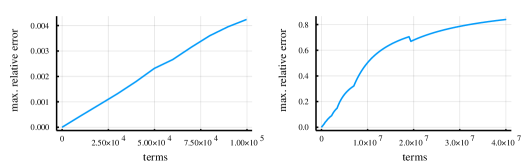
Figure 1: Measured error in the evaluation of the sequence $(c_{n})$ defined by (18) in IEEE binary32 floating-point arithmetic ($u=2^{-24}\simeq 6\cdot 10^{-8}$). For each $n$, we plot the maximum observed error on $c_{n}$ for 997 exactly representable values of $c_{0}$ regularly spaced in the interval $[\pi/2,\pi]$. The script used to produce these plots is available in the supplementary material.

Figure 1 illustrates, on two different scales, the accumulation of errors in numerical experiments. We can see that the relative error actually growths roughly linearly until it saturates around $1$ (meaning that the computed results no longer have a single correct significant digit but remain of the correct order of magnitude). Thus the bounds (24), (25) are still very pessimistic compared to reality. This was to be expected: indeed, it would be quite surprising for all local errors $\varepsilon_{n}$ to align to reach the worst case rather than be more or less evenly distributed in $[-u,u]$. The standard model does not capture this fact. We refer to Higham [20, Section 2.8] and Higham and Mary [21] for a discussion of the kinds of bounds that can be derived if one is willing to make assumptions on the distribution of individual rounding errors.

Remark 9.1.

Starting back from (20), one may be tempted to write the partial fraction decomposition of $\hat{\delta}(z)$ and deduce an exact formula for $\hat{\delta}_{n}$. Doing so leads to

$$\hat{\delta}_{n}=(A\alpha^{n}-B\beta^{n}-u^{-1}n)\mathopen{|}c_{0}\mathclose{|}u,\qquad A=\frac{\alpha^{3}}{(\alpha-1)^{2}(\alpha-\beta)},\quad B=A-1-u^{-1}.$$

This expression is misleading, for it involves cancellations between terms that tend to infinity as $u$ goes to zero. In particular, we have $A\sim\frac{1}{2}u^{-3/2}$ as $u\rightarrow 0$.

10 Relative Errors, Infinite Order: Scaled Bernoulli Numbers

For a more sophisticated application of the same idea, let us study the floating-point computation of scaled Bernoulli numbers as described by Brent [6, Section 7] (see also Brent and Zimmermann [8, Section 4.7.2]). This section is the first where not only the method but the results are new.

The scaled Bernoulli numbers are defined in terms of the classical Bernoulli numbers $B_{k}$ by $b_{k}=B_{2k}/(2k)!$. Their generating series has a simple explicit expression:

(26) $$b(z)=\sum_{k=0}^{\infty}b_{k}z^{k}=\frac{\sqrt{z}/2}{\tanh\left(\sqrt{z}/2\right)}.$$

One possible algorithm for computing $b_{k}$, suggested by Reinsch according to Brent [6, Section 12], is to follow the recurrence

(27) $$b_{k}=\frac{1}{(2k)!4^{k}}-\sum_{j=0}^{k-1}\frac{b_{j}}{(2k+1-2j)!4^{k-j}}.$$

In [8, Exercise 4.35], it is asked to “prove (or give a plausibility argument for)” the fact that the relative error on $b_{k}$ when computed using (27) in floating-point arithmetic is $\mathrm{O}(k^{2}u)$. The $\mathrm{O}(k^{2}u)$ bound is already mentioned without proof in [6], and again in [7, Section 2]. Paul Zimmermann (private communication, June 2018) suggested that the dependency in $k$ may actually be linear rather than quadratic.

Our goal in this section is to prove a version of the latter conjecture. Like in the previous section, it cannot be true if the $\mathrm{O}(\cdot)$ is interpreted as uniform as $u\rightarrow 0$ and $k\rightarrow\infty$ independently. It does hold, however, when $u$ and $k$ are restricted to a region where their product is small enough, as well as in the sense that the relative error $\eta_{k}$ for fixed $k$ satisfies $\mathopen{|}\eta_{k}\mathclose{|}\leqslant C_{k}u$ when $u$ is small enough, for a sequence $C_{k}$ which itself satisfies $C_{k}=\mathrm{O}(k)$ as $k\rightarrow\infty$. We will in fact derive a fully explicit, non-asymptotic bound in terms of $u$ and $k$.

Based on the form of (26), denote $w=\sqrt{z}/2$, and for any $f\in\mathbb{C}[[z]]$, define $f^{\ast}$ by $f^{\ast}(w)=f(4w^{2})$, so that $f^{\ast}(w)=f(z)$. In particular, we have $b^{\ast}(w)=w/\tanh w$. We will use the following classical facts about the numbers $|b_{k}|$.

Lemma 10.1.

The absolute values of the scaled Bernoulli numbers satisfy

$${}^{\sharp}b^{\ast}(w)=2-\frac{w}{\tan w},\qquad\mathopen{|}b_{k}\mathclose{|}\sim_{k\rightarrow\infty}\frac{2}{(2\pi)^{2k}},\qquad\frac{2}{(2\pi)^{2k}}\leqslant\mathopen{|}b_{k}\mathclose{|}\leqslant\frac{4}{(2\pi)^{2k}},$$

where the last formula assumes $k\geqslant 1$.

Proof 10.2.

The expression of ${}^{\sharp}b^{\ast}(w)$ can be deduced from that of $b^{\ast}(w)$ and the fact that $B_{2n}$ has sign $(-1)^{n+1}$ for $n\geqslant 1$, using the relation $\tanh(iw)=i\tan(w)$. The other statements follow from the expression of Bernoulli numbers using the Riemann zeta function [[, e.g.,]formula (25.6.2)]DLMF.

Let $\tilde{b}_{k}$ denote the approximate value of $b_{k}$ computed using (27). We assume that the computed value of $n!$ is equal to $n!/(1+q_{n})$ with $q_{n}=\theta_{n-2}$, in the notation of Section 7, for $n\geqslant 2$, and $q_{0}=q_{1}=1$. According to the modified standard model of floating-point arithmetic, this holds true if $n!$ is computed as $(((2\times 3)\times 4)\times\cdots\times n)$ and the working precision is at least $\lceil\log_{2}n\rceil$, even with no special treatment of multiplications by powers of two. The local error introduced by one step of the iteration (27) then behaves as follows.

Lemma 10.3.

At every step of the iteration (27), the computed value $\tilde{b}_{k}$ has the form

(28) $$\tilde{b}_{k}=\frac{1+s_{k}}{(2k)!4^{k}}-\sum_{j=0}^{k-1}\frac{\tilde{b}_{j}(1+t_{k,j})}{(2k+1-2j)!4^{k-j}},\qquad\mathopen{|}s_{k}\mathclose{|}\leqslant\hat{\theta}_{2k},\quad\mathopen{|}t_{k,j}\mathclose{|}\leqslant\hat{\theta}_{3(k-j)+2}.$$

Proof 10.4.

The computation of $b_{0}$ ($=1$) involves no rounding error. Assume $k\geqslant 1$, and first consider the term $a_{k}=1/((2k)!4^{k})$ outside the sum. By assumption, the computed value of $(2k)!$ is $(2k)!/(1+q_{2k})$, and the multiplication by $4^{k}$ that follows is exact. Inverting the result introduces an additional rounding error. The computed value of the whole term is hence $a_{k}(1+r_{k}^{\prime})$ where $r_{k}^{\prime}=\theta_{2k-1}$. By the same reasoning, the term of index $j$ in the sum is computed with a relative error $r_{k,j}=\theta_{2(k-j)+1}$ for all $j,k$. If $v_{k,i}$ denotes the relative error in the addition of the term of index $i$ to the partial sum for $0\leqslant j\leqslant i-1$, the computed value of the sum is hence

$$\sum_{j=0}^{k-1}\frac{\tilde{b}_{j}(1+r_{k,j})}{(2k+1-2j)!4^{k-j}}\prod^{k-1}_{i=j}(1+v_{k,i}).$$

Taking into account the relative error $v^{\prime}_{k}$ of the final subtraction leads us to (28), with

$$1+s_{k}=(1+r^{\prime}_{k})(1+v^{\prime}_{k}),\qquad 1+t_{k,j}=(1+r_{k,j})(1+v^{\prime}_{k})\prod^{k-1}_{i=j}(1+v_{k,i}),$$

which concludes the proof.

Let $\delta_{k}=\tilde{b}_{k}-b_{k}$. Comparison of (28) with (27) yields

$$\delta_{k}=\frac{s_{k}}{(2k)!4^{k}}-\sum_{j=0}^{k-1}\frac{\delta_{j}+\tilde{b}_{j}t_{k,j}}{(2k+1-2j)!4^{k-j}},$$

which rearranges into

(29) $$\sum_{j=0}^{k}\frac{\delta_{j}}{(2k+1-2j)!4^{k-j}}=\frac{s_{k}}{(2k)!4^{k}}-\sum_{j=0}^{k-1}\frac{(b_{j}+\delta_{j})t_{k,j}}{(2k+1-2j)!4^{k-j}}.$$

Using the bounds from Lemma 10.3, with  $\hat{\theta}_{3(k-j)+2}$ replaced by $\hat{\theta}_{4(k-j)+2}$ to obtain slightly simpler expressions later, it follows that

(30) $$\left|\sum_{j=0}^{k}\frac{\delta_{j}}{(2k+1-2j)!4^{k-j}}\right|\leqslant\frac{\hat{\theta}_{2k}}{(2k)!4^{k}}+\sum_{j=0}^{k-1}\frac{(\mathopen{|}b_{j}\mathclose{|}+\mathopen{|}\delta_{j}\mathclose{|})\hat{\theta}_{4(k-j)+2}}{(2k+1-2j)!4^{k-j}}.$$

Let us introduce the auxiliary series

$$C(z)=\sum_{k=0}^{\infty}\frac{z^{k}}{(2k)!4^{k}}=\cosh w,\quad S(z)=\sum_{k=0}^{\infty}\frac{z^{k}}{(2k+1)!4^{k}}=\frac{\sinh w}{w},\quad\check{S}(z)=\frac{w}{\sin w},$$

$$\tilde{C}(z)=\hat{\theta}^{(2,0)}(z)\odot C(z),\quad\tilde{S}(z)=\hat{\theta}^{(4,2)}(z)\odot(S(z)-1).$$

The inequality (30) (note that the sum on the right-hand side stops at $k-1$) translates into

$$\delta(z)S(z)\ll\tilde{C}(z)+\tilde{S}(z)\left({}^{\sharp}b(z)+{}^{\sharp}\delta(z)\right).$$

Since $\check{S}(z)$ has nonnegative coefficients [35, (4.19.4)], we have $S(z)^{-1}=iw/\sin(iw)\ll\check{S}(z)$, hence

$$\delta(z)\ll\check{S}(z)\tilde{C}(z)+\check{S}(z)\tilde{S}(z){}^{\sharp}b(z)+\check{S}(z)\tilde{S}(z){}^{\sharp}\delta(z).$$

As $\tilde{S}(z)=\mathrm{O}(z)$, Lemma 6.3 applies and yields

(31) $$\delta(z)\ll\hat{\delta}(z):=\frac{\check{S}(z)\tilde{C}(z)+\check{S}(z)\tilde{S}(z){}^{\sharp}b(z)}{1-\check{S}(z)\tilde{S}(z)}.$$

Using Lemma 7.2 to rewrite the Hadamard products, we have

(32) $$\tilde{C}(z) =C(a^{2}z)-C(z)=\cosh(aw)-\cosh(w),$$

(33) $$\tilde{S}(z) =a^{2}S(a^{4}z)-S(z)-(a^{2}-1)=\frac{\sinh(a^{2}w)-\sinh(w)}{w}-(a^{2}-1),$$

where $a=1+u$. In addition, Lemma 10.1 gives a formula for ${}^{\sharp}b(z)$. Thus (31) yields an explicit, if complicated, majorant series for $\delta(z)$.

It is not immediately clear how to extract a readable bound on $\delta_{k}$ in the style of (23). However, we can already prove an asymptotic version of Zimmermann’s observation. The calculations leading to Propositions 10.5 and 10.9 can be checked with the help of a computer algebra system. A worksheet that illustrates how to do that using Maple is provided in the supplementary material.

Proposition 10.5.

When $k$ is fixed and for small enough $u$, the relative error $\eta_{k}=\delta_{k}/b_{k}$ satisfies $\mathopen{|}\eta_{k}\mathclose{|}\leqslant C_{k}u$ for some $C_{k}$. In addition, the constants $C_{k}$ can be chosen such that $C_{k}=\mathrm{O}(k)$ as $k\rightarrow\infty$.

Proof 10.6.

As $u$ tends to zero, we have

$$\hat{\delta}(z) =\left(\frac{2(1-\cosh w)\cos(w)}{w^{-2}\sin(w)^{2}}+\frac{4(\cosh w-1)+w\sinh w}{w^{-1}\sin w}\right)u+\mathrm{O}(u^{2})$$

$$=:\hat{\xi}(z)u+\mathrm{O}(u^{2}),$$

where the coefficients are to be interpreted as formal series in $z$. Hence, for fixed $k$, the error $\delta_{k}$ is bounded by $\hat{\xi}_{k}u+\mathrm{O}(u^{2})$ as $u\rightarrow 0$. The function $\hat{\xi}^{\ast}(w)$ is meromorphic, with double poles at $w=\pm\pi$, corresponding for $\hat{\xi}(z)$ to a unique pole of minimal modulus (also of order two) at $z=4\pi^{2}$. This implies (by Lemma 5.1) that $(2\pi)^{2k}\hat{\xi}_{k}=\mathrm{O}(k)$ as $k\rightarrow\infty$. The result follows using the growth estimates from Lemma 10.1.

In other words, there exist a constant $A$ and a function $R$ such that $\eta_{k}\leqslant Aku+R(k,u)$, where $R(k,u)=o(u)$ as $u\rightarrow 0$ for fixed $k$, but $R(k,u)$ might be unbounded if $k$ tends to infinity while $u$ tends to zero. (Remark 10.13 below shows that an exponential dependency in $k$ is in fact unavoidable.) To get a bound valid for all $u$ and $k$ in a reasonable region, let us study the denominator of (31) more closely. A similar argument applied to $\hat{\xi}$ in the place of $\hat{\delta}$ would make the constant $A$ explicit.

Lemma 10.7.

For small enough $u\geqslant 0$, the function $h:w\mapsto\tilde{S}^{\ast}(w)-\check{S}^{\ast}(w)^{-1}$ has exactly two simple zeros $\pm\alpha=\pm\pi/(1+\varphi(u))$ closest to the origin, with

(34) $$\varphi(u)=2(\cosh(\pi)-1)u+\mathrm{O}(u^{2}),\quad u\rightarrow 0.$$

Furthermore, if $u\leqslant 2^{-16}$, then one has $0\leqslant\varphi(u)\leqslant 2(\cosh(\pi)-1)u$, and $h$ has no other zero than $\pm\alpha$ in the disk $\mathopen{|}w\mathclose{|}<\rho:=6.2$.

Proof 10.8.

To start with, observe that when $u=0$, the term $\tilde{S}^{\ast}(w)$ in the definition of $h$ vanishes identically, leaving us with $h(w)=\check{S}^{\ast}(w)^{-1}=w^{-1}\sin w$. The zeros of $1/\check{S}^{\ast}$ closest to the origin are located at $w=\pm\pi$, the next closest, at $w=\pm 2\pi$ and hence outside the disk $\mathopen{|}w\mathclose{|}<\rho$.

Let us focus on the zero at $w=\pi$. Since $h^{\prime}(\pi)=1/\pi$ for $u=0$, the Implicit Function Theorem applies and shows that, locally, the zero varies analytically with $u$. One obtains the asymptotic form (34) by implicit differentiation.

We turn to the bounds on $\varphi(u)$. The power series expansion of $\tilde{S}^{\ast}$ with respect to $w$ has nonnegative coefficients, showing that $h(\pi)=\tilde{S}^{\ast}(\pi)\geqslant 0$. Now, with $a=1+u$ as in (33), isolate the first nonzero term of that series and write

$$\tilde{S}^{\ast}(w)=\frac{a^{6}-1}{6}w^{2}+\frac{G(a^{2}w)-G(w)}{w},\qquad G(w)=\sinh(w)-w-\frac{w^{3}}{6}.$$

Let $K=2(\cosh(\pi)-1)$ and $w_{0}=\pi/(1+Ku)$. One has

(35) $$G(a^{2}w_{0})-G(w_{0})\leqslant(a^{2}-1)w_{0}\max_{1\leqslant t\leqslant a^{2}}\mathopen{|}G^{\prime}(tw_{0})\mathclose{|}.$$

Note that $a^{2}w_{0}\leqslant\pi$ for all $u\leqslant 1/2$. Since $G(w)\gg 0$, it follows that

$$G(a^{2}w_{0})-G(w_{0})\leqslant(a^{2}-1)w_{0}G^{\prime}(\pi),$$

therefore the term $\tilde{S}^{\ast}(w_{0})$ in $h(w_{0})$ satisfies

$$\tilde{S}^{\ast}(w_{0})\leqslant\frac{a^{6}-1}{6}w_{0}^{2}+(a^{2}-1)G^{\prime}(\pi).$$

As for the other term, the inequality $\sin(\pi-v)\geqslant v-v^{3}/6$ ($u\geqslant 0$) applied to $v=\pi-w_{0}=Kuw_{0}$ yields

$$-\check{S}^{\ast}(w_{0})^{-1}\leqslant-Ku+(Ku)^{3}\frac{w_{0}^{2}}{6}.$$

Collecting both contributions and substituting in the value $G^{\prime}(\pi)=(K-\pi^{2})/2$, we obtain

$$h(w_{0})\leqslant\hat{h}:=\frac{a^{6}-1}{6}\frac{\pi^{2}}{(1+Ku)^{2}}+\frac{a^{2}-1}{2}(K-\pi^{2})-Ku+(Ku)^{3}\frac{w_{0}^{2}}{6}.$$

The right-hand side is an explicit rational function of $u$, satisfying

$$\hat{h}\sim(-2\pi^{2}(K-1)+K/2)u^{2}$$

as $u\rightarrow 0$. One can check that it remains negative for $0<u\leqslant 2^{-16}$. Thus, one has $h(w_{0})<0\leqslant h(\pi)$, and $h$ has a zero in the interval $w\in[w_{0},\pi]$, that is, a zero of the form $\alpha=\pi/(1+\varphi(u))$ with $0\leqslant\varphi(u)\leqslant Ku$, as claimed. The corresponding statement for $-\alpha$ follows by parity.

It remains to show that $\pm\alpha$ are the only zeros of $h$ in the disk $\mathopen{|}w\mathclose{|}<\rho$. We do it by comparing them to the zeros of $1/\check{S}^{\ast}$ using Rouché’s theorem.

To this end, note first that the expression $\mathopen{|}\sin(\rho e^{i\theta})\mathclose{|}$ reaches its minimum for $\theta\in[0,\pi/2]$ when $\theta=0$. Indeed, one has $\mathopen{|}\sin(\rho e^{i\theta})\mathclose{|}^{2}=\cosh(\rho\sin\theta)^{2}-\cos(\rho\cos\theta)^{2}$. The term $\cosh(\rho\sin\theta)^{2}$ is strictly increasing on the whole interval. For $\theta\leqslant\theta_{0}:=\arccos(3\pi/(2\rho))$, the term $-\cos(\rho\cos\theta)^{2}$ is increasing as well, so that $\mathopen{|}\sin(\rho e^{i\theta})\mathclose{|}\geqslant\mathopen{|}\sin\rho\mathclose{|}$ in that range, whereas for $\theta_{0}\leqslant\theta\leqslant\pi$, we have $\mathopen{|}\sin(\rho e^{i\theta})\mathclose{|}^{2}\geqslant\cosh(\rho\sin\theta_{0})^{2}-1>1\geqslant\mathopen{|}\sin\rho\mathclose{|}^{2}$. It follows that $\mathopen{|}\sin w\mathclose{|}\geqslant\mathopen{|}\sin\rho\mathclose{|}$, and hence $\mathopen{|}\check{S}^{\ast}(w)^{-1}\mathclose{|}\geqslant\rho^{-1}\mathopen{|}\sin\rho\mathclose{|}$, for $w=\rho e^{i\theta}$ with $0\leqslant\theta\leqslant\pi/2$, and by symmetry on the whole circle $\mathopen{|}w\mathclose{|}=\rho$.

Turning to $\tilde{S}^{\ast}(w)$ and reasoning as in (35) starting from (33), one can write

$$\mathopen{|}\tilde{S}^{\ast}(w)\mathclose{|}\leqslant(a^{2}-1)\sup_{1\leqslant t\leqslant a^{2}}\mathopen{|}\cosh(tw)-1\mathclose{|}\leqslant(a^{2}-1)\cosh(a^{2}\rho)$$

for $\mathopen{|}w\mathclose{|}=\rho$. Comparing these bounds leads to

$$\mathopen{|}\tilde{S}^{\ast}(w)\mathclose{|}<10^{-2}<\mathopen{|}\check{S}^{\ast}(w)^{-1}\mathclose{|},\qquad\mathopen{|}w\mathclose{|}=\rho,\quad 0\leqslant u\leqslant 2^{-16}.$$

Therefore, $h(w)$ has the same number of zeros as $w^{-1}\sin w$ inside the circle.

Proposition 10.9.

For all $0<u\leqslant 2^{-16}$, we have $\tilde{b}_{k}=b_{k}(1+\eta_{k})$ where

$$\mathopen{|}\eta_{k}\mathclose{|}\leqslant(1+21.2u)^{k}(1.1k+446)u.$$

Proof 10.10.

We use the notation of the previous lemma. In the expression (31) of $\hat{\delta}(z)$, the series $\tilde{S}(z)$ and $\tilde{C}(z)$ define entire functions, while ${}^{\sharp}b^{\ast}(w)=2-w/\tan w$ is a meromorphic function with poles at $w\in\pi\mathbb{Z}$. These observations combined with Lemma 10.7 imply that $\hat{\delta}^{\ast}$ is meromorphic in the disk $\mathopen{|}w\mathclose{|}<6.2$, with exactly four simple poles located at $w=\pm\alpha$ and $w=\pm\pi$. Only the first two poles depend on $u$.

One has $\hat{\delta}^{\ast}(w)\sim-(1-w/\pi)^{-1}$ as $w\rightarrow\pi$. Let $F^{\ast}$ denote the derivative of $w\mapsto w\tilde{S}^{\ast}(w)$. With the help of a computer algebra system, it is not too hard to determine that the singular expansion as $w\rightarrow\alpha$ reads

$$\hat{\delta}^{\ast}(w)\sim\frac{\tilde{C}^{\ast}(\alpha^{2})-\cos\alpha+2\alpha^{-1}\sin\alpha}{F^{\ast}(\alpha)-\cos\alpha}\frac{1}{1-w/\alpha}=:\frac{R(u)}{1-w/\alpha}$$

and one has $R(u)=1+(2\cosh\pi-2-\pi\sinh\pi)u+\mathrm{O}(u^{2})$ as $u\rightarrow 0$. The expansions at $-\alpha$ and $-\pi$ follow since $\hat{\delta}^{\ast}$ is an even function. Set

$$\hat{\delta}^{\ast}(w)=\frac{R(u)}{1-w/\alpha}+\frac{R(u)}{1+w/\alpha}-\frac{1}{1-w/\pi}-\frac{1}{1+w/\pi}+g^{\ast}(u,w),$$

where $g^{\ast}(u,\cdot)$ now is analytic for $\mathopen{|}w\mathclose{|}<6.2\approx 1.97\pi$ and vanishes identically when $u=0$. Since

$$\frac{R(u)}{1\pm w/\alpha}-\frac{1}{1\pm w/\pi}=\frac{R(u)-1}{1\pm w/\alpha}\mp\frac{\varphi(u)w/\pi}{(1\pm w/\alpha)(1\pm w/\pi)},$$

we have

$$\hat{\delta}^{\ast}(w)=\frac{2(R(u)-1)}{1-(w/\alpha)^{2}}+\frac{2\varphi(u)(2+\varphi(u))(w/\pi)^{2}}{(1-(w/\alpha)^{2})(1-(w/\pi)^{2})}+g^{\ast}(u,w),$$

that is,

$$\hat{\delta}(z)=\frac{2(R(u)-1)}{1-z/(2\alpha)^{2}}+\frac{2\varphi(u)(2+\varphi(u))z/(2\pi)^{2}}{(1-z/(2\alpha)^{2})(1-z/(2\pi)^{2})}+g(u,z).$$

By Cauchy’s inequality, for any $\lambda<1.9$, the Taylor coefficients $g_{k}$ of $g(u,\cdot)$ satisfy

$$\mathopen{|}g_{k}\mathclose{|}\leqslant\frac{A_{\lambda}(u)}{(2\pi\lambda)^{2k}},\qquad A_{\lambda}(u):=\max_{\text{\scriptsize{$\begin{array}[]{c}\mathopen{|}w\mathclose{|}=\lambda\pi\end{array}$}}}\mathopen{|}g^{\ast}(u,w)\mathclose{|},$$

and therefore

(36) $$\hat{\delta}(z)\ll\frac{2\mathopen{|}R(u)-1\mathclose{|}}{1-z/(2\alpha)^{2}}+\frac{2\varphi(u)(2+\varphi(u))z/(2\alpha)^{2}}{(1-z/(2\alpha)^{2})^{2}}+\frac{A_{\lambda}(u)}{1-z/(2\pi\lambda)^{2}},$$

where we have bounded $\nu z/(1-\nu z)$ where $\nu=1/(2\pi)^{2}$ by the same expression with $\nu=1/(2\alpha)^{2}$.

For $0\leqslant u\leqslant 2^{-16}$ and using the enclosure of $\varphi(u)$ from Lemma 10.7, a brute force evaluation using interval arithmetic yields the bounds

$$\mathopen{|}R(u)-1\mathclose{|}\leqslant(\max_{0\leqslant v\leqslant u}\mathopen{|}R^{\prime}(v)\mathclose{|})u\leqslant 72u,\qquad\frac{2\varphi(u)(2+\varphi(u))}{(2\alpha)^{2}}\leqslant 2.2u.$$

SageMath code for computing these estimates can be found in the supplementary material. By the same method, choosing $\lambda=\sqrt{3/2}$ and making use of the fact that $g^{\ast}(0,w)=0$, we get

$$A_{\lambda}(u)\leqslant u\max_{\text{\scriptsize{$\begin{array}[]{c}0\leqslant v\leqslant u\\ \mathopen{|}w\mathclose{|}=\lambda\pi\end{array}$}}}\left|\frac{\partial g^{\ast}}{\partial u}(v,w)\right|\leqslant 747u.$$

We substitute these bounds in (36) to conclude that

$$\hat{\delta}_{k} \leqslant(2\times 72(2\alpha)^{-2k}+2.2k(2\alpha)^{-2k}+747(2\pi\lambda)^{-2k})u$$

$$\leqslant\frac{1}{(2\pi)^{2k}}((2.2k+2\times 72)(1+2(\cosh\pi-1)u)^{2k}+747(2/3)^{k})u$$

$$\leqslant\frac{(1+21.2u)^{2k}}{(2\pi)^{2k}}(2.2k+891)u.$$

The claim follows since, as noted in Lemma 10.1, $\mathopen{|}b_{k}\mathclose{|}\geqslant 2(2\pi)^{-2k}$ for all $k\geqslant 1$.

Corollary 10.11.

For all $u$ and $k$ satisfying $0<u\leqslant 2^{-16}$ and $43ku\leqslant 1$, one has $\tilde{b}_{k}=b_{k}(1+\eta_{k})$ with $\mathopen{|}\eta_{k}\mathclose{|}\leqslant(3k+1213)u$.

Proof 10.12.

The assumption on $ku$ implies $(1+21.2u)^{2k}\leqslant e$.

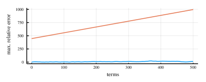
Figure 2: Bound from Proposition 10.9 (top curve) and measured error (bottom curve), in multiples of the unit roundoff $u$, for the evaluation of the scaled Bernoulli numbers in 53-bit floating-point arithmetic with unbounded exponents. The script used to produce this plot is available in the supplementary material.

Proposition 10.9 and Corollary 10.11 seem difficult to improve significantly, at least if we keep reasoning analytically, without bringing into play the discrete low-level behavior of rounding errors. Figure 2 illustrates that, as in the previous section, the bounds nevertheless overestimate the actual accumulated errors.

Remark 10.13.

Let us now prove our claim that no bound of the form $\eta_{k}=\mathrm{O}(ku)$ can hold uniformly with respect to $u$ and $k$. In the notation of Lemma 10.3, suppose that we have $s_{k}=u$ and $t_{k,j}=\hat{\theta}_{k-j}$ for all $k,j$. These values are reached, e.g., by taking $v_{k,i}=u$ and $v^{\prime}_{k}=r_{k,j}=r^{\prime}_{k}=0$ for all $i,j,k$. Since the $v_{k,i}$ and $v^{\prime}_{k}$ represent individual rounding errors, this corresponds to a feasible situation in our model. Then, (29) translates into $\delta(z)S(z)=C(z)u-(\hat{\theta}\odot S)(z)(b(z)+\delta(z))$, that is,

$$\delta(z)=\frac{C(z)u-\bigl{(}S((1+u)z)-S(z)\bigr{)}b(z)}{S((1+u)z)}.$$

For small $u$, the denominator vanishes at $z=\beta:=-4\pi^{2}/(1+u)$, while the numerator is analytic for $\mathopen{|}w\mathclose{|}<\pi$ and does not vanish at $\beta$ (it tends to $-1$ as $u\rightarrow 0$, since $S(\beta)\sim u/2$ and $\delta(\beta)\sim-2u^{-1}$). Thus, the radius of convergence of $\delta(z)$ is at most $4\pi^{2}/(1+u)$. This implies that $\eta_{k}$ grows exponentially for fixed $u$.

11 Two Variables: The Equation of a Vibrating String

As part of an interesting case study of formal program verification in scientific computing, Boldo et al. [3, 5, 4] give a full worst-case rounding error analysis of a simple explicit finite difference scheme for the one-dimensional wave equation

(37) $$\frac{\partial^{2}p}{\partial t^{2}}-c^{2}\frac{\partial^{2}p}{\partial x^{2}}=0.$$

Such a finite difference scheme is nothing but a multi-dimensional linear recurrence—in the present case, a two-dimensional one, with a time index ranging over the natural numbers while the space index is restricted to a finite domain. We rephrase the relatively subtle error analysis using a slight extension of the language introduced in the previous sections. Doing so does not change the essence of the argument, but possibly makes it more palatable.

We use the notation and assumptions of [5, Section 3.2], [4, Section 5], except that we flip the sign of $\delta_{i}^{k}$ to keep with our usual conventions. Time and space are discretized into a grid with time step $\Delta t$ and space step $\Delta x$. To the continuous solution $p(x,t)$ corresponds a double sequence $(p_{i}^{k})$ where $k\geqslant 0$ is the space index and $0\leqslant i\leqslant n$ is the time index. Taking central differences for the derivatives in (37) and letting $a=(c\Delta t/\Delta x)^{2}$ leads to

(38) $$\left\{\begin{aligned} p_{i}^{1}&=p_{i}^{0}+\dfrac{a}{2}(p_{i+1}-2p_{i}+p_{i-1}),&\\ p_{i}^{k+1}&=2p_{i}^{k}-p_{i}^{k-1}+a(p_{i+1}^{k}-2p_{i}^{k}+p_{i-1}^{k}),&&k\geqslant 1.\end{aligned}\right.$$

The problem is subject to the boundary conditions $p_{0}^{k}=p_{n}^{k}=0$, $k\in\mathbb{N}$, and we are given initial data $(p_{i}^{0})_{i=1}^{n-1}$. In accordance with the Courant-Friedrichs-Lewy condition, we assume $0<a\leqslant 1$.

Boldo et al. study an implementation of (38) in double-precision floating-point arithmetic, but their focus is on the propagation of absolute errors. Their local error analysis shows that the computed values $(\tilde{p}_{i}^{k})$ corresponding to $(p_{i}^{k})$ satisfy

(39) $$\left\{\begin{aligned} \tilde{p}_{i}^{0}&=p_{i}^{0}+\delta_{i}^{0}\\ \tilde{p}_{i}^{1}&=\tilde{p}_{i}^{0}+\dfrac{a}{2}(\tilde{p}_{i+1}^{0}-2\tilde{p}_{i}^{0}+\tilde{p}_{i-1}^{0})+\delta_{i}^{1}-\left(\delta_{i}^{0}+\dfrac{a}{2}(\delta_{i+1}^{0}-2\delta_{i}^{0}+\delta_{i-1}^{0})\right),\\ \tilde{p}_{i}^{k+1}&=2\tilde{p}_{i}^{k}-\tilde{p}_{i}^{k-1}+a(\tilde{p}_{i+1}^{k}-2\tilde{p}_{i}^{k}+\tilde{p}_{i-1}^{k})+\delta_{i}^{k+1},\qquad k\geqslant 1\end{aligned}\right.$$

with $\mathopen{|}\delta_{i}^{k}\mathclose{|}\leqslant\bar{\delta}:=78\cdot 2^{-52}$ for all $i$ and all $k\geqslant 1$. While the discussion of error propagation in [5, 4] assumes $\delta_{i}^{0}=0$, the machine-checked proof actually allows for initial errors $\mathopen{|}\delta_{i}^{0}\mathclose{|}\leqslant\bar{\delta}^{0}:=14\cdot 2^{-52}$ and gives the additional bound $\mathopen{|}\delta_{i}^{1}\mathclose{|}\leqslant\bar{\delta}^{1}:=81\cdot 2^{-53}$. Both in [5, 4] and here, the computation of these local bounds is the only step of the analysis that depends on the assumption that the computation is run in double precision.

From there, they prove [4, Theorem 5.2] that one has $\mathopen{|}\tilde{p}_{i}^{k}-p_{i}^{k}\mathclose{|}\leqslant\frac{1}{2}\bar{\delta}(k+1)(k+2)$ for all $i$ and $k$. (As usual, a naive analysis would lead to an exponential bound.) The main aim of this section is to give a new proof of this result.

The iterations (38) and (39) are, a priori, valid for $0<i<n$ only, but it is not hard to see that they can be made to hold for all $i\in\mathbb{Z}$ by extending the sequences $(p_{i}^{k})$, $(\tilde{p}_{i}^{k})$, and $(\delta_{i}^{k})$ by odd symmetry and $(2n)$-periodicity with respect to $i$. Viewing time as the main variable, we encode space-periodic sequences of period $2n$ by generating series of the form

(40) $$f(x,t)=\sum_{k=0}^{\infty}\sum_{i=-n}^{n-1}f_{i}^{k}x^{i}t^{k}\in\Omega[[t]]$$

where $\Omega=\mathbb{R}[x]/\langle x^{2n}-1\rangle$ is the ring of polynomials modulo $x^{2n}-1$. When $f$ is an element of $\Omega[[t]]$, we denote

$$f^{u:}(x,t)=\sum_{k\geqslant u}\sum_{i}f_{i}^{k}x^{i}t^{k},\qquad f_{i}(t)=\sum_{k}f_{i}^{k}t^{k},\qquad f^{k}(x)=\sum_{i}f_{i}^{k}x^{i}.$$

Multiplication by $x$ and $t$ in $\Omega[[t]]$ respectively corresponds to backward shifts of the indices $i$ and $k$.

Let $\Delta(x,t)=\tilde{p}(x,t)-p(x,t)$ (where $\Delta$, $\tilde{p}$, and $p$ all are special cases of (40)) be the generating series of the global error. Our goal is to obtain bounds on the $\Delta_{i}^{k}$. We start by expressing $\Delta(x,t)$ in terms of $\delta(x,t)$. This is effectively a more precise version of [4, Theorem 5.1] covering initial data with numeric errors.

Proposition 11.1.

One has

(41) $$\Delta(x,t)=\lambda(x,t)\eta(x,t)$$

where

(42) $$\lambda(x,t)=\frac{1}{1-\varphi(x)t+t^{2}},\qquad\eta(x,t)=\delta(x,t)-\varphi(x)t\delta_{0}(x)$$

with

$$\varphi(x)=2+a(x^{-1}-2+x).$$

Proof 11.2.

By comparing (39) with (38) and observing how $\Delta_{i}^{1}$ simplifies thanks to the correcting term in $\tilde{p}_{i}^{1}$, we get

(43) $$\left\{\begin{aligned} \Delta_{i}^{k}&=\delta_{i}^{k},&&k=0,1,\\ \Delta_{i}^{k+1}&=2\Delta_{i}^{k}-\Delta_{i}^{k-1}+a(\Delta_{i+1}^{k}-2\Delta_{i}^{k}+\Delta_{i-1}^{k})+\delta_{i}^{k+1},&&k+1\geqslant 2.\end{aligned}\right.$$

In terms of series, (43) translates into

(44) $$\Delta^{0}(x)=\delta^{0}(x),\qquad\Delta^{1}(x)=\delta^{1}(x),$$

(45) $$t^{-1}\Delta^{2:}(x,t)=2\Delta^{1:}(x,t)-t\Delta(x,t)+a(x^{-1}-2+x)\Delta^{1:}(x,t)+t^{-1}\delta^{2:}(x,t).$$

Taking into account (44), equation (45) becomes

$$\Delta(x,t)=2t(\Delta(x,t)-\delta_{0}(x))-t^{2}\Delta(x,t)+a(x^{-1}-2+x)t(\Delta(x,t)-\delta^{0}(x))+\delta(x,t),$$

that is,

$$(1-(2+a(x^{-1}-2+x))t+t^{2})\Delta(x,t)=\delta(x,t)-\varphi(x)t\delta_{0}(x)$$

The coefficient on the left-hand side is invertible in $\Omega[[t]]$, leading to the equality $\Delta(x,t)={\lambda(x,t)}\eta(x,t)$.

Rather than by bivariate majorant series, we will control elements of $\Omega[[t]]$ by majorant series in a single variable relative to a norm on $\Omega$. We say that $\hat{f}\in\mathbb{R}_{\geqslant 0}[[t]]$ is a majorant series of $f\in A[[t]]$ with respect to a norm $\|{\cdot}\|_{s}$ on an algebra $A$, and write $f\ll_{s}\hat{f}$, when $\|f_{k}\|_{s}\leqslant\hat{f}_{k}$ for all $k\in\mathbb{N}$. The basic properties listed in Section 6 extend in the obvious way. In particular, if $\|{\cdot}\|_{q},\|{\cdot}\|_{r},\|{\cdot}\|_{s}$ are norms such that $\|uv\|_{q}\leqslant\|u\|_{r}\|v\|_{s}$, then $f\ll_{r}\hat{f}$ and $g\ll_{s}\hat{g}$ imply $fg\ll_{q}\hat{f}\hat{g}$.

For $u=\sum_{i}u_{i}x^{i}\in\Omega$, we define

$$\|u\|_{1}=\sum_{i=-n}^{n-1}\mathopen{|}u_{i}\mathclose{|},\qquad\|u\|_{2}=\left(\sum_{i=-n}^{n-1}\mathopen{|}u_{i}\mathclose{|}^{2}\right)^{1/2},\qquad\|u\|_{\infty}=\max_{i=-n}^{n-1}\mathopen{|}u_{i}\mathclose{|}.$$

Note the inequality $\|uv\|_{\infty}\leqslant\|u\|_{1}\|v\|_{\infty}$ for $u,v\in\Omega$ (an instance of Young’s convolution inequality).

The local error analysis yields

$$\delta(x,t)\ll_{\infty}\bar{\delta}^{0}+\bar{\delta}^{1}t+\frac{\bar{\delta}t^{2}}{1-t}.$$

Using the notation of Proposition 11.1, one has $\|\varphi(x)\|_{1}\leqslant 2$, hence $\|\varphi(x)\delta^{0}(x)\|_{\infty}\leqslant 2\bar{\delta}^{0}$ and

(46) $$\eta(x,t)\ll_{\infty}\bar{\delta}^{0}+(\bar{\delta}^{1}+2\bar{\delta}_{0})t+\frac{\bar{\delta}t^{2}}{1-t}\ll\frac{\bar{\delta}}{1-t}.$$

We first deduce a bound on the global error in quadratic mean with respect to space. We will later get a second proof of this result as a corollary of Proposition 11.6; the main interest of the present one is that it does not rely on Lemma 11.5.

Proposition 11.3.

One has

$$\Delta(x,t)\ll_{2}\frac{\sqrt{2n}}{(1-t)^{3}}\bar{\delta}.$$

In other words, the root mean square error at time $k$ satisfies

$$\left(\frac{1}{n}\sum_{i=0}^{n-1}(\Delta_{i}^{k})^{2}\right)^{1/2}\leqslant\frac{(k+1)(k+2)}{2}\bar{\delta}.$$

Proof 11.4.

Elements of $\Omega$ can be evaluated at $2n$-th roots of unity, and the collection $u^{\ast}=(u(\omega))_{\omega^{2n}=1}$ of values of a polynomial $u\in\Omega$ is nothing but the discrete Fourier transform of its coefficients. The coefficientwise Fourier transform of formal power series,

$$f(t)\mapsto f^{\ast}(t)=(f(\omega,t))_{\omega^{2n}=1},$$

is an algebra homomorphism from $\Omega[[t]]$ to $\mathbb{C}^{2n}[[t]]$. One easily checks Parseval’s identity for the discrete Fourier transform:

$$\|u\|_{2}=\frac{1}{\sqrt{2n}}\|u^{\ast}\|_{2},\qquad u\in\Omega,$$

where the norm on the right-hand side is the standard Euclidean norm on $\mathbb{C}^{2n}$.

The uniform bound (46) resulting from the local error analysis implies

$$\eta(x,t)\ll_{2}\frac{\sqrt{2n}}{1-t}\bar{\delta},$$

and Parseval’s identity yields

$$\eta^{\ast}(t)\ll_{2}\frac{2n\bar{\delta}}{1-t}.$$

At $x=\omega=e^{\mathrm{i}\theta}$, the factor $\lambda$ in (41) takes the form

$$\lambda(\omega,t)=\frac{1}{1-2b_{\omega}t+t^{2}},\qquad b_{\omega}=1+a(\cos\theta-1),$$

where $-1\leqslant b_{\omega}\leqslant 1$ due to the assumption that $0<a\leqslant 1$. The denominator therefore factors as $(1-\zeta_{\omega}t)(1-\bar{\zeta}_{\omega}t)$ where $\mathopen{|}\zeta_{\omega}\mathclose{|}=1$, so that we have

$$\lambda(\omega,t)=\frac{1}{(1-\zeta_{\omega}t)(1-\bar{\zeta}_{\omega}t)}\ll\frac{1}{(1-t)^{2}}$$

in $\mathbb{C}[[t]]$ and hence $\lambda^{\ast}(t)\ll_{\infty}(1-t)^{-2}$.

Since the entrywise product in $\mathbb{C}^{2n}$ satisfies $\|u^{\ast}v^{\ast}\|_{2}\leqslant\|u^{\ast}\|_{\infty}\|v^{\ast}\|_{2}$, the bounds on $\lambda^{\ast}$ and $\eta^{\ast}$ combine into

$$\lambda^{\ast}(t)\eta^{\ast}(t)\ll_{2}\frac{2n\bar{\delta}}{(1-t)^{3}}.$$

Using Parseval’s identity again, we conclude that

$$\Delta(x,t)=\lambda(x,t)\eta(x,t)\ll_{2}\frac{\sqrt{2n}\bar{\delta}}{(1-t)^{3}}$$

as claimed. The second formulation of the result comes from the symmetry of the data: one has $\Delta(x^{-1},t)=-\Delta(x,t)$, hence $\|\Delta^{k}\|_{2}^{2}=2\sum_{i=0}^{n-1}(\Delta_{i}^{k})^{2}$ for all $k$.

Proposition 11.3 immediately implies $\Delta(x,t)\ll_{\infty}\bar{\delta}\sqrt{2n}(1-t)^{-3}$. However, this estimate turns out to be too pessimistic by a factor $\sqrt{2n}$. The key to better bounds is the following lemma, proved (with the help of generating series!) in Appendix C of [4]. The argument, due to M. Kauers and V. Pillwein, reduces the problem to an inequality of Askey and Gasper via an explicit expression in terms of Jacobi polynomials that is proved using Zeilberger’s algorithm. It remains intriguing to find a more direct way to derive the uniform bound on $\Delta$.

Lemma 11.5.

The coefficients $\lambda_{i}^{k}$ of $\lambda(x,t)$ are nonnegative.

Strictly speaking, the nonnegativity result in [4] is about the coefficients, not of $\lambda(x,t)\in\Omega[[t]]$ as defined above, but of its lift to $\mathbb{R}[x,x^{-1}][[t]]$ obtained by interpreting (42) in the latter ring. It is thus slightly stronger than the above lemma.

From this lemma it is easy to deduce a more satisfactory bound on the global error, matching that of [4, Theorem 5.2].

Proposition 11.6.

One has the bound

$$\Delta(x,t)\ll_{\infty}\frac{\bar{\delta}}{(1-t)^{3}},$$

that is,

$$\mathopen{|}\Delta_{i}^{k}\mathclose{|}\leqslant\frac{1}{2}\bar{\delta}(k+1)(k+2)$$

for all $i$ and $k$.

Proof 11.7.

Lemma 11.5 implies $\lambda(x,t)\ll_{1}\lambda(1,t)$. This bound combines with (46) to give

$$\Delta(x,t)=\lambda(x,t)\eta(x,t)\ll_{\infty}\lambda(1,t)\frac{\bar{\delta}}{(1-t)}=\frac{\bar{\delta}}{(1-t)^{3}},$$

just like in the proof of Proposition 11.3.

12 Solutions of Linear Differential Equations

For the last application, we return to recurrences of finite order in a single variable. Instead of looking at a specific sequence, though, we now consider a general class of recurrences with polynomial coefficients. It is technically simpler and quite natural to restrict our attention to recurrences associated to nonsingular differential equations under the correspondence from Lemma 4.2: thus, we consider a linear ordinary differential equation

(47) $$p_{r}(z)y^{(r)}(z)+\cdots+p_{1}(z)y^{\prime}(z)+p_{0}(z)y(z)=0$$

where $p_{0},\ldots,p_{r}\in\mathbb{C}[z]$ and assume that $p_{r}(0)\neq 0$. We expect that this assumption could be lifted by working along the lines of [32].

It is classical that (47) then has $r$ linearly independent formal power series solutions and all these series are convergent in a neighborhood of $0$. Suppose that we want to evaluate one of these solutions at a point lying within its disk of convergence. A natural way to proceed is to sum the series iteratively, using the associated recurrence to generate the coefficients. Our goal in this section is to give an error bound on the approximation of the partial sum computed by a version of this algorithm. We do not consider the truncation error here (see however Remark 12.5 below).

We formulate the computation as an algorithm based on interval arithmetic that returns an enclosure of the partial sum. Running the whole loop in interval arithmetic would typically lead to enclosures of width that growths exponentially with the number of computed terms, and thus to a catastrophic loss of accuracy. Instead, the algorithm executes the body of the loop in interval arithmetic, which saves us from going into the details of the local error analysis, but “squashes” the computed interval to its midpoint after each loop iteration. It maintains a running bound on the discarded radii that serves to control the overall effect of the propagation of local errors. This way of using interval arithmetic does not create long chains of interval operations depending on each other and only produces a small overestimation.

The procedure is presented as Algorithm 1. While, to the best of our knowledge, the algorithm is new, the approach just sketched is a very natural one. The main contribution of this section is the automated error analysis that makes it applicable.

In the algorithm and the analysis that follows, we use the notation of Section 4 for differential and recurrence operators, with the symbol $\partial$ denoting $\mathrm{d}/\mathrm{d}z$. When $P=p_{r}\partial^{r}+\cdots$ is a differential operator, we denote by

$$\rho(P)=\min\{\mathopen{|}\xi\mathclose{|}:p_{r}(\xi)=0\}\in[0,\infty]$$

the radius of the disk centered at the origin and extending to the nearest singular point. Variable names set in bold represent complex intervals, or balls, and operations involving them obey the usual laws of midpoint-radius interval arithmetic (i.e., $\boldsymbol{x}\ast\boldsymbol{y}$ is a reasonably tight ball containing $x\ast y$, for all $x\in\boldsymbol{x}$, $y\in\boldsymbol{y}$, and for every arithmetic operation $\ast$). We denote by $\operatorname{mid}(\boldsymbol{x})$ the center of a ball $\boldsymbol{x}$ and by $\operatorname{rad}(\boldsymbol{x})$ its radius.

Algorithm 1

Input

An operator $P=p_{r}(z)\partial^{r}+\cdots+p_{1}(z)\partial+p_{0}(z)$, with $p_{r}(0)\neq 0$. A vector $(\boldsymbol{u}_{n})_{n=0}^{r-1}$ of ball initial values. An evaluation point $\zeta\in\mathbb{C}$ with $\mathopen{|}\zeta\mathclose{|}<\rho(P)$. A truncation order $N$.

Output

A complex ball containing $\sum_{n=0}^{N-1}u_{n}\zeta^{n}$, where $u(z)$ is the solution of $P\cdot u=0$ corresponding to the given initial values.

1. [Compute a recurrence relation.] Define $L\in\mathbb{K}[X][Y]$ by $z^{r}P=L(z,z\partial)$. Compute polynomials $b_{0}(n),\ldots,b_{s}(n)$ such that

   $$L(S^{-1},n)=b_{0}(n)-b_{1}(n)S^{-1}-\cdots-b_{s}(n)S^{-s}.$$

2. [Compute a majorant differential equation.] Let $m=\max(1,\deg p_{r})$. Compute a rational $\alpha\approx\rho(P)^{-1}$ such that $\rho(P)^{-1}<\alpha<\mathopen{|}\zeta\mathclose{|}^{-1}$. (If $\rho(P)=\infty$, take, for instance, $\alpha\approx\mathopen{|}\zeta\mathclose{|}^{-1}/2$.) Compute rationals $c\approx\mathopen{|}p_{r}(0)\mathclose{|}$ and $M$ such that $0<c\leqslant\mathopen{|}p_{r}(0)\mathclose{|}$ and $M\geqslant\max_{i=0}^{r-1}\sum_{j=0}^{\deg p_{i}}\mathopen{|}p_{i,j}\mathclose{|}\alpha^{-i-j-1}$.

3. [Initial values for the bounds.] Compute positive lower bounds on the first $r$ terms of the series $\hat{g}(z)=\exp\left(Mc^{-1}\alpha\int_{0}^{z}(1-\alpha z)^{-m}\right)$. (This is easily done using arithmetic on truncated power series with ball coefficients.) Deduce rationals $\hat{u}_{0}\geqslant\max_{n=0}^{r-1}(\mathopen{|}\boldsymbol{u}_{n}\mathclose{|}/\hat{g}_{n})$ and $\hat{\delta}_{0}\geqslant\max_{n=0}^{r-1}(\mathopen{|}\delta_{n}\mathclose{|}/\hat{g}_{n})$.

4. [Initialize the recurrence.] Set

   $$(\tilde{u}_{r-s},\ldots,\tilde{u}_{-1},\tilde{u}_{0},\ldots,\tilde{u}_{r-1})=(0,\ldots,0,\operatorname{mid}(\boldsymbol{u}_{0}),\ldots,\operatorname{mid}(\boldsymbol{u}_{r-1})),$$

   $\boldsymbol{s}_{0}=0$, $\boldsymbol{t}_{0}=1$, $\bar{\eta}=0$. (Although most variables are indexed by functions on $n$ for ease of reference, only $(\tilde{u}_{n-i})_{i=0}^{s}$, $\boldsymbol{s}_{n}$, $\boldsymbol{t}_{n}$, and $\bar{\eta}$ need to be stored from one loop iteration to the next.)

5. For $n=1,\ldots,N$, do:

   1. If $n\geqslant r$, then:

      1. [Next coefficient.] Compute

         $$\boldsymbol{u}_{n}=\dfrac{1}{b_{0}(n)}(b_{1}(n)\tilde{u}_{n-1}+\cdots+b_{s}(n)\tilde{u}_{n-s})$$

         in ball arithmetic.

      2. [Round.] Set $\tilde{u}_{n}=\operatorname{mid}(\boldsymbol{u}_{n})$. (If $\boldsymbol{u}_{n}$ contains $0$, it can be better in practice to force $\tilde{u}_{n}$ to $0$ even if $\operatorname{mid}(\boldsymbol{u}_{n})\neq 0$ and increase $\operatorname{rad}(\boldsymbol{u}_{n})$ accordingly.)

      3. [Local error bound.] Let $\mu=\mathopen{|}\tilde{u}_{n-1}\mathclose{|}+\cdots+\mathopen{|}\tilde{u}_{n-s}\mathclose{|}$. If $\mu\neq 0$, then update $\bar{\eta}$ to $\max(\bar{\eta},\eta_{n})$ where $\eta_{n}=\operatorname{rad}(\boldsymbol{u}_{n})/\mu$.

   2. [Next partial sum.] Compute $\boldsymbol{t}_{n}=\zeta\cdot\boldsymbol{t}_{n-1}$ and $\boldsymbol{s}_{n}=\boldsymbol{s}_{n-1}+\tilde{u}_{n-1}\boldsymbol{t}_{n-1}$ using ball arithmetic.

6. [Account for accumulated numerical errors.] Compute $\sigma\geqslant c(\mathopen{|}\zeta\mathclose{|}+\cdots+\mathopen{|}\zeta\mathclose{|}^{s})$. If $\sigma\bar{\eta}\geqslant 1$, signal an error. Otherwise, compute

   (48) $$A\geqslant\frac{M\alpha\mathopen{|}\zeta\mathclose{|}}{(1-\alpha\mathopen{|}\zeta\mathclose{|})^{m}},\qquad\Delta_{N}\geqslant\frac{\hat{\delta}_{0}+\hat{u}_{0}\sigma(1+A)\bar{\eta}}{1-\sigma\bar{\eta}}\exp\frac{A}{1-\sigma\bar{\eta}}$$

   and increase the radius of $\boldsymbol{s}_{N}$ by $\Delta_{N}$.

7. Return $\boldsymbol{s}_{N}$.

As mentioned, the key feature of Algorithm 1 is that step 5(a)1 computes $\boldsymbol{u}_{n}$ based only on the centers of the intervals $\boldsymbol{u}_{n-1},\ldots,\boldsymbol{u}_{n-s}$, ignoring their radii. In the remainder of this section, we will prove that thanks to the correction made at step 6, the enclosure returned when the computation succeeds is nevertheless correct. The algorithm may also fail at step 6, but that can always be avoided by increasing the working precision (provided that interval operations on inputs of radius tending to zero produce results of radius that tends to zero).

With the notation from the algorithm, let $u(z)$ be a power series solution of $P\cdot u=0$ corresponding to initial values $u_{0}\in\boldsymbol{u}_{0},\ldots,u_{r}\in\boldsymbol{u}_{r}$. The Cauchy existence theorem implies that such a solution exists and that $u(z)$ converges on the disk $\mathopen{|}z\mathclose{|}<\rho(P)$. We recall basic facts about the recurrence obtained at step 1. Let $Q(X)=X(X-1)\cdots(X-r+1)$.

Lemma 12.1.

The coefficient sequence $(u_{n})$ of $u(z)$ satisfies

(49) $$b_{0}(n)u_{n}=b_{1}(n)u_{n-1}+\cdots+b_{s}(n)u_{n-s},\nopagebreak$$

where one has $b_{0}(n)=p_{r}(0)Q(n)$. In particular, $b_{0}$ is not the zero polynomial.

Proof 12.2.

Observe that for $p\in\mathbb{C}[z]$, the operator $\partial p=p\partial+p^{\prime}$ has $p$ as a leading coefficient when viewed as a polynomial in $\partial$ with coefficients in $\mathbb{C}[z]$ written to the left. It follows that $z^{k}\partial^{k}=(z\partial)^{k}+\left(\text{terms involving lower powers of\leavevmode\nobreak\ $\partial$}\right)$ and therefore that $z^{r}P$ can be written as a polynomial in $z$ and $z\partial$, as implicitly required by the algorithm. That the operator $L(S^{-1},n)$ annihilates $(u_{n})$ follows from Lemma 4.2.

The only term of $z^{r}P$, viewed as a sum of monomials $p_{i,j}z^{j}\partial^{i}$ that can contribute to $b_{0}$ is $p_{r}(0)z^{r}\partial^{r}$, for all others have $i-j<0$. The relation $z^{k}\partial^{k}=(z\partial-{k+1})z^{k-1}\partial^{k-1}$ then shows that $b_{0}(n)=p_{r}(0)Q(n)$, where $p_{0}(0)\neq 0$ by assumption.

Let $\hat{a}(z)=Mc^{-1}\alpha(1-\alpha z)^{-m}$ where $M$, $c$, and $\alpha$ are the quantities computed at step 2 of the algorithm.

Lemma 12.3.

Let $y,\hat{y}$ be power series such that $P\cdot y\ll\partial^{r-1}(\partial-\hat{a})\cdot\hat{y}$. If one has $\mathopen{|}y_{n}\mathclose{|}\leqslant\hat{y}_{n}$ for $n<r$, then $y\ll\hat{y}$.

Proof 12.4.

Let $\hat{P}=\partial^{r-1}(\partial-\hat{a}(z))$, that is,

$$\hat{P}=\partial^{r-1}\left(\partial-\frac{Mc^{-1}\alpha}{(1-\alpha z)^{m}}\right)=\partial^{r}-\sum_{i=0}^{r-1}\hat{f}_{i}(z)\partial^{r-1-i}$$

where

$$\hat{f}_{i}(z)=\binom{r-1}{i}\frac{(m+i-1)!}{(m-1)!}\frac{Mc^{-1}\alpha^{i+1}}{(1-\alpha z)^{m+i}}.$$

The parameters $c$, $m$, and $\alpha$ are chosen so that $(1-\xi^{-1}z)^{-1}\ll(1-\alpha z)^{-1}$ for every root $\xi$ of $p_{r}$, and hence $p_{r}(z)^{-1}\ll c^{-1}(1-\alpha z)^{-m}$. Since, additionally, one has $(\alpha z)^{j}(1-\alpha z)^{-1}\ll(1-\alpha z)^{-1}$, it follows that, for $0\leqslant i<r$,

$$\frac{p_{i}(z)}{p_{r}(z)}\ll\frac{\sum_{j}\mathopen{|}p_{i,j}\mathclose{|}z^{j}}{c(1-\alpha z)^{m}}=\sum_{j}\mathopen{|}p_{i,j}\mathclose{|}\alpha^{-j}\frac{(\alpha z)^{j}}{c(1-\alpha z)^{m}}\ll\frac{Mc^{-1}\alpha^{i+1}}{(1-\alpha z)^{m}}\ll\hat{f}_{i}(z),$$

by definition of $M$. By Proposition 6.5, these inequalities and our assumptions on $\hat{y}$ imply that one has ${y\ll\hat{y}}$.

Lemma 12.3 applies in particular to series $y,\hat{y}$ with $P\cdot y=0$ and $\hat{y}^{\prime}=\hat{a}\hat{y}$. The solution $\hat{g}$ of the latter equation with $\hat{g}_{0}=1$ is the series

(50) $$\hat{g}(z)=\exp\int_{0}^{z}\hat{a}(w)\mathrm{d}w$$

already encountered at step 3 of the algorithm. Observe that none of its coefficients vanishes. Therefore, step 3 runs without error, and ensures that $\mathopen{|}u_{n}\mathclose{|}\leqslant\hat{u}_{0}\hat{g}_{n}$ (and $\mathopen{|}\delta_{n}\mathclose{|}\leqslant\hat{\delta}_{0}\hat{g}_{n}$) for $n<r$. As $P\cdot u=0$, the lemma implies $u\ll\hat{u}_{0}\hat{g}$.

Remark 12.5.

Therefore, the tails of the series $\hat{u}(z)=\hat{u}_{0}\hat{g}(z)$ determined by Algorithm 1 are majorant series of the tails of $u(z)$. This means that the algorithm can be modified to simultaneously bound the truncation and rounding error, and most of the steps involved can be shared between both bounds. We refer the reader to [31] and the references therein for more on the computation of tight bounds on truncation errors. Though our focus here is on the propagation of local errors, the modified algorithm is the more interesting one for applications in rigorous computing, for it can serve as the basic brick of an algorithm for computing rigorous enclosures of solutions of ODEs with polynomial coefficients.

Let us now turn to the loop. As usual, consider the computed coefficient sequence $(\tilde{u}_{n})$, and let $\delta_{n}=\tilde{u}_{n}-u_{n}$. Write

$$\tilde{u}_{n}=\dfrac{1}{b_{0}(n)}(b_{1}(n)\tilde{u}_{n-1}+\cdots+b_{s}(n)\tilde{u}_{n-s})+\varepsilon_{n},\qquad r\leqslant n\leqslant N,$$

so that $\mathopen{|}\varepsilon_{n}\mathclose{|}\leqslant\operatorname{rad}(\boldsymbol{u}_{n})$. Let $\eta_{n}=\varepsilon_{n}/(\mathopen{|}\tilde{u}_{n-1}\mathclose{|}+\cdots+\mathopen{|}\tilde{u}_{n-s}\mathclose{|})$ when $r\leqslant n\leqslant N$ and the denominator is nonzero, and $\eta_{n}=0$ otherwise. We thus have, for all $n\in\mathbb{Z}$,

(51) $$b_{0}(n)\tilde{u}_{n}-b_{1}(n)\tilde{u}_{n-1}-\cdots-b_{s}(n)\tilde{u}_{n-s}=b_{0}(n)\eta_{n}(\mathopen{|}\tilde{u}_{n-1}\mathclose{|}+\cdots+|\tilde{u}_{n-s}|)$$

and, thanks to step 5(a)3 of the algorithm, $\mathopen{|}\eta_{n}\mathclose{|}\leqslant\bar{\eta}$. By subtracting (49) from (51) and bounding $\eta_{n}$ by $\bar{\eta}$, we obtain

(52) $$\mathopen{|}b_{0}(n)\delta_{n}-b_{1}(n)\delta_{n-1}-\cdots-b_{s}(n)\delta_{n-s}\mathclose{|}\leqslant c\bar{\eta}Q(n)(\mathopen{|}\tilde{u}_{n-1}\mathclose{|}+\cdots+\mathopen{|}\tilde{u}_{n-s}\mathclose{|}).$$

Let $\varphi(z)=z+\cdots+z^{s}$.

Lemma 12.6.

Let $\hat{v}\in\mathbb{R}_{\geqslant 0}[[z]]$ be any majorant series of $(\varphi\,{}^{\sharp}u)^{\prime}(z)$. The equation

(53) $$(1-c\bar{\eta}\varphi(z))\hat{\delta}^{\prime}(z)=(\hat{a}(z)+c\bar{\eta}\varphi^{\prime}(z))\hat{\delta}(z)+c\bar{\eta}\hat{v}(z).$$

admits a solution $\hat{\delta}(z)$ with the initial value $\hat{\delta}_{0}$ computed at step 3, and this solution is a majorant series of $\delta(z)$.

Proof 12.7.

In terms of generating series, (52) rewrites as $z^{r}P\cdot\delta(z)\ll c\bar{\eta}Q(z\partial)\varphi(z)\cdot{}^{\sharp}\tilde{u}(z)$. As already observed in the proof of Lemma 12.1, one has $Q(z\partial)=z^{r}\partial^{r}$, so that the previous equation is equivalent to

(54) $$P\cdot\delta(z)\ll c\bar{\eta}\partial^{r}\varphi(z)\cdot{}^{\sharp}\tilde{u}(z).$$

Let $\hat{\gamma}$ be the solution of

(55) $$(\partial-\hat{a}(z))\cdot\hat{\gamma}(z)=c\bar{\eta}\partial\varphi(z)\cdot{}^{\sharp}\tilde{u}(z)$$

with $\hat{\gamma}_{0}=\hat{\delta}_{0}$. By Proposition 6.5, we have $\hat{\delta}_{0}\hat{g}(z)\ll\hat{\gamma}(z)$ where $\hat{g}$ is given by (50). In addition, as noted when discussing step 3, we have $\mathopen{|}\delta_{n}\mathclose{|}\leqslant\hat{\delta}_{0}\hat{g}_{n}$ for $n<r$, hence $\mathopen{|}\delta_{n}\mathclose{|}\leqslant\hat{\gamma}_{n}$ for $n<r$. As $\hat{\gamma}$ also satisfies $P\cdot\delta\ll\partial^{r}(\partial-\hat{a})\cdot\hat{\gamma}$, we can conclude that $\delta\ll\hat{\gamma}$ using Lemma 12.3. But then, since $\tilde{u}=u+\delta$, we have ${}^{\sharp}\tilde{u}\ll{}^{\sharp}u+\hat{\gamma}$, hence $\left(\varphi{}^{\sharp}\tilde{u}\right)^{\prime}\ll\hat{v}+(\varphi\hat{\gamma})^{\prime}$, and (55) implies

$$\hat{\gamma}^{\prime}=\hat{a}\hat{\gamma}+c\bar{\eta}\left(\varphi{}^{\sharp}\tilde{u}\right)^{\prime}\ll c\bar{\eta}\varphi\hat{\gamma}^{\prime}+(\hat{a}+c\bar{\eta}\varphi^{\prime})\hat{\gamma}+c\bar{\eta}\hat{v}$$

where we note that $\varphi(0)=0$. This inequality is of the form required by Lemma 6.7, which yields the existence of $\hat{\delta}$ and the inequality $\hat{\gamma}\ll\hat{\delta}$. We thus have $\delta\ll{\hat{\gamma}\ll\hat{\delta}}$.

It remains to solve the majorant equation (53) to get an explicit bound on $\hat{\delta}$.

Proposition 12.8.

The generating series $\delta(z)$ of the global error on $u_{n}$ committed by Algorithm 1 satisfies

(56) $$\delta(z)\ll\frac{\hat{\delta}_{0}+c\bar{\eta}\hat{u}_{0}\varphi(z)(1+z\hat{a}(z))}{1-c\bar{\eta}\varphi(z)}\exp\left(\frac{z\hat{a}(z)}{1-c\bar{\eta}\varphi(z)}\right),\quad\hat{a}(z)=\frac{Mc^{-1}\alpha}{(1-\alpha z)^{m}}.$$

Proof 12.9.

The solution $\hat{h}(z)$ of the homogeneous part of (53) with $\hat{h}_{0}=1$ is given by

$$\hat{h}(z)=\frac{1}{1-c\bar{\eta}\varphi(z)}\exp\int_{0}^{z}\frac{\hat{a}(w)}{1-c\bar{\eta}\varphi(w)}\mathrm{d}w.$$

Observe that

$$\left(\varphi{}^{\sharp}u\right)^{\prime}\ll\hat{u}_{0}(\varphi\hat{g})^{\prime}=\hat{u}_{0}(\varphi^{\prime}+\varphi\hat{a})\hat{g}\ll\hat{u}_{0}(\varphi^{\prime}+\varphi\hat{a})\hat{h},$$

so that, in Lemma 12.6, we can take $\hat{v}(z)=\hat{u}_{0}(\varphi^{\prime}+\varphi\hat{a})\hat{h}$. The method of variation of parameters then leads to the expression

$$\hat{\delta}(z)=\hat{h}(z)\left(\hat{\delta}_{0}+c\bar{\eta}\int_{0}^{z}\frac{\hat{v}(w)}{\hat{h}(w)}\mathrm{d}w\right)=\hat{h}(z)\left(\hat{\delta}_{0}+c\bar{\eta}\hat{u}_{0}\left(\varphi(z)+\int_{0}^{z}\varphi(w)\hat{a}(w)\mathrm{d}w\right)\right).$$

Using the bounds from Lemma 6.9

$$\int_{0}^{z}\frac{\hat{a}(w)}{1-c\bar{\eta}\varphi(w)}\mathrm{d}w\ll\frac{z\hat{a}(z)}{1-c\bar{\eta}\varphi(z)},\qquad\int_{0}^{z}\varphi(w)\hat{a}(w)\mathrm{d}w\ll z\varphi(z)\hat{a}(z),$$

we see that $\hat{\delta}(z)$ is bounded by the right-hand side of (56). Note in passing that $z\hat{a}(z)$ could be replaced by $\int_{0}^{z}\hat{a}$ at the price of a slightly more complicated final bound.

Step 6 of Algorithm 1 effectively computes an upper bound on $\mathopen{|}\delta(\zeta)\mathclose{|}$ using inequality (56). It follows that the returned interval $\boldsymbol{s}_{N}$ contains the exact partial sum $\sum_{n=0}^{N-1}u_{n}\zeta^{n}$ corresponding to the input data, as stated in the specification of the algorithm. This concludes the proof of correctness of Algorithm 1.

Remark 12.10.

Instead of $\varepsilon_{n}/(\mathopen{|}\tilde{u}_{n-1}\mathclose{|}+\cdots+\mathopen{|}\tilde{u}_{n-s}\mathclose{|})$, one could compute a run-time bound directly on $\mathopen{|}\varepsilon_{n}/\hat{h}_{n}\mathclose{|}$. Doing so leads to a somewhat simpler variant of the above analysis. We chose to present the version given here because it is closer to plain floating-point error analysis — and gives us an excuse to illustrate the generalization to recurrences with polynomial coefficients of the technique of Section 9. Another small advantage is that plugging in a sharper first-order majorant equation as suggested below requires no other change to the algorithm, whereas it may not be obvious how to compute a good lower bound on $\hat{h}_{n}$.

It is natural to ask how this algorithm compares to naive interval summation. We limit ourselves to a short informal discussion. When the operator $P$, the series $u(z)$ and the evaluation point $\zeta$ are fixed, our bound $\Delta_{N}$ on the global error decreases linearly with $\hat{\delta}_{0}+\bar{\eta}$. Suppose that we run the algorithm with a relative working precision of $t$ bits. Under the reasonable assumptions that $\operatorname{rad}(\boldsymbol{u}_{n})=\mathrm{O}(2^{-t})$ for $0\leqslant n<r$ and that both $\eta_{n}$ and $\operatorname{rad}(\boldsymbol{s}_{n})$ are $\mathrm{O}(n^{d}2^{-t})$ for some $d$, we then have $\Delta_{N}=\mathrm{O}(N^{d}2^{-t})$. As the truncation order $N$ necessary for reaching an accuracy $\mathopen{|}\boldsymbol{s}_{N}-u(\zeta)\mathclose{|}\leqslant 2^{-q}$ is $N=\mathrm{O}(q)$, this means that, for fixed $u$ and $\zeta$, the algorithm needs no more than $q+\mathrm{O}(\log q)$ bits of working precision to compute an enclosure of $u(\zeta)$ of width $2^{-q}$. In the same setting, computing the partial sum purely in ball arithmetic (that is, without Step 5(a)2 of Algorithm 1) may require a working precision of the order of $q+\lambda N$ bits, for some $\lambda$ depending on the recurrence.

The majorant series of Proposition 12.8 was chosen to keep the algorithm simple, not to optimize the error bound, so that we do not expect the version described here to be practical. One helpful feature it does have is that the parameter $\alpha$ can be taken arbitrarily close to $\rho(p_{r})^{-1}$ without forcing other parts of the bound to tend to infinity. (This is in contrast with the geometric majorant series typically found in textbook proofs of theorems on differential equations.) Nevertheless, the exponential factor in (48) can easily grow extremely large, and we expect Algorithm 1 to lead to unusable bounds in practice on moderately complicated examples. Even in simple cases, forcing a majorant series of finite radius of convergence when $p_{r}$ is constant is far from optimal.

The same idea, though, can be used with a more sophisticated choice of majorant series. In particular, the algorithm adapts without difficulty if $\hat{a}(z)$ is a sharper rational majorant of the coefficients of the equation. As a first step toward making the algorithm practical, we have implemented a variant based on the more flexible framework of [31], in the ore_algebra package [28, 30] for SageMath. Preliminary experiments suggest that, in some cases, it is very effective in reducing the working precision necessary for computing enclosures of solutions of differential equations with polynomial coefficients. At this stage, though, it does not consistently run faster than naive interval summation, due both to overestimation issues and to the computational overhead of obtaining good bounds. We leave it to future work to develop an efficient Taylor method for solving linear ODEs with polynomial incorporating the technique presented in this section. It would also be interesting to extend the analysis to the computation of “logarithmic series” solutions of linear ODEs at regular singular points.

References

• [1] R. Barrio, B. Melendo and S. Serrano “On the numerical evaluation of linear recurrences” In Journal of Computational and Applied Mathematics 150.1, 2003, pp. 71–86 DOI: 10.1016/S0377-0427(02)00565-4
• [2] Roberto Barrio “Rounding error bounds for the Clenshaw and Forsythe algorithms for the evaluation of orthogonal polynomial series” In Journal of Computational and Applied Mathematics 138.2, 2002, pp. 185–204 DOI: 10.1016/S0377-0427(01)00382-X
• [3] Sylvie Boldo “Floats and Ropes: A Case Study for Formal Numerical Program Verification” In Automata, Languages and Programming, Lecture Notes in Computer Science Springer, 2009, pp. 91–102 DOI: 10.1007/978-3-642-02930-1_8
• [4] Sylvie Boldo et al. “Trusting Computations: A Mechanized Proof from Partial Differential Equations to Actual Program” In Computers & Mathematics with Applications 68.3, 2014, pp. 325–352 DOI: 10.1016/j.camwa.2014.06.004
• [5] Sylvie Boldo et al. “Wave Equation Numerical Resolution: A Comprehensive Mechanized Proof of a C Program” In Journal of Automated Reasoning 50.4, 2013, pp. 423–456 DOI: 10.1007/s10817-012-9255-4
• [6] Richard P. Brent “Unrestricted Algorithms for Elementary and Special Functions” In Information Processing 80, 1980 URL: https://maths-people.anu.edu.au/~brent/pub/pub052.html
• [7] Richard P. Brent and David Harvey “Fast Computation of Bernoulli, Tangent and Secant Numbers” In Computational and Analytical Mathematics New York, NY: Springer, 2013, pp. 127–142 DOI: 10.1007/978-1-4614-7621-4_8
• [8] Richard P. Brent and Paul Zimmermann “Modern Computer Arithmetic” Cambridge University Press, 2010 URL: https://members.loria.fr/PZimmermann/mca/pub226.html
• [9] Henri Cartan “Théorie élémentaire des fonctions analytiques d’une ou plusieurs variables complexes” Hermann, 1961
• [10] Augustin Cauchy “Mémoire sur l’emploi du nouveau calcul, appelé calcul des limites, dans l’intégration d’un système d’équations différentielles” In Comptes-rendus de l’Académie des Sciences 15, 1842, pp. 14
• [11] Augustin Cauchy “Œuvres complètes d’Augustin Cauchy, Ière série” Gauthier-Villars, 1892 URL: https://gallica.bnf.fr/ark:/12148/bpt6k901870
• [12] Augustin Cauchy “Résumé d’un mémoire sur la Mécanique céleste et sur un nouveau calcul appelé calcul des limites” In Exercices d’analyse et de physique mathématique II Bachelier, 1841, pp. 50–109
• [13] C.. Clenshaw “A note on the summation of Chebyshev series” In Mathematics of Computation 9, 1955, pp. 118–120 URL: http://www.ams.org/journals/mcom/1955-09-051/S0025-5718-1955-0071856-0/
• [14] Roger Cooke “The Cauchy–Kovalevskaya Theorem” URL: https://web.archive.org/web/20100725150116/http://www.cems.uvm.edu/~cooke/ckthm.pdf
• [15] David Elliott “Error analysis of an algorithm for summing certain finite series” In Journal of the Australian Mathematical Society 8.2, 1968, pp. 213–221 DOI: 10.1017/S1446788700005267
• [16] Philippe Flajolet and Robert Sedgewick “Analytic Combinatorics” Cambridge University Press, 2009 URL: http://algo.inria.fr/flajolet/Publications/book.pdf
• [17] M. Giusti, G. Lecerf, B. Salvy and J.-C. Yakoubsohn “On Location and Approximation of Clusters of Zeros of Analytic Functions” In Foundations of Computational Mathematics 5.3, 2005, pp. 257–311 DOI: 10.1007/s10208-004-0144-z
• [18] Joseph F. Grcar “John von Neumann’s Analysis of Gaussian Elimination and the Origins of Modern Numerical Analysis” In SIAM Review 53.4, 2011, pp. 607–682 DOI: 10.1137/080734716
• [19] Peter Henrici “Discrete Variable Methods in Ordinary Differential Equations” Wiley, 1962
• [20] Nicholas J. Higham “Accuracy and stability of numerical algorithms” SIAM, 2002
• [21] Nicholas J. Higham and Theo Mary “A New Approach to Probabilistic Rounding Error Analysis” In SIAM Journal on Scientific Computing 41.5 Society for IndustrialApplied Mathematics, 2019, pp. A2815–A2835 DOI: 10.1137/18M1226312
• [22] Thibault Hilaire and Benoit Lopez “Reliable Implementation of Linear Filters with Fixed-Point Arithmetic” In SiPS 2013 Proceedings, 2013, pp. 401–406 DOI: 10.1109/SiPS.2013.6674540
• [23] Einar Hille “Ordinary differential equations in the complex domain” Wiley, 1976
• [24] Joris Hoeven “Majorants for formal power series”, 2003 URL: http://www.texmacs.org/joris/maj/maj-abs.html
• [25] Tomasz Hrycak and Sebastian Schmutzhard “Evaluation of Chebyshev polynomials by a three-term recurrence in floating-point arithmetic” In BIT Numerical Mathematics 58.2, 2018, pp. 317–330 DOI: 10.1007/s10543-017-0683-8
• [26] Fredrik Johansson and Marc Mezzarobba “Fast and Rigorous Arbitrary-Precision Computation of Gauss–Legendre Quadrature Nodes and Weights” In SIAM Journal on Scientific Computing 40.6, 2018, pp. C726–C747 DOI: 10.1137/18M1170133
• [27] Manuel Kauers “The holonomic toolkit” In Computer Algebra in Quantum Field Theory: Integration, Summation and Special Functions, Texts and Monographs in Symbolic Computation Springer, 2013 URL: http://www.risc.jku.at/people/mkauers/publications/kauers13.pdf
• [28] Manuel Kauers, Maximilian Jaroschek and Fredrik Johansson “Ore polynomials in Sage” In Computer Algebra and Polynomials Springer, 2015, pp. 105–125 DOI: 10.1007/978-3-319-15081-9_6
• [29] B. Liu and T. Kaneko “Error Analysis of Digital Filters Realized with Floating-Point Arithmetic” In Proceedings of the IEEE 57.10, 1969, pp. 1735–1747 DOI: 10.1109/PROC.1969.7388
• [30] Marc Mezzarobba “Rigorous Multiple-Precision Evaluation of D-Finite Functions in SageMath” Extended abstract of a talk at the 5th International Congress on Mathematical Software, 2016 URL: http://arxiv.org/abs/1607.01967
• [31] Marc Mezzarobba “Truncation Bounds for Differentially Finite Series” In Annales Henri Lebesgue 2 ÉNS Rennes, 2019, pp. 99–148 DOI: 10.5802/ahl.17
• [32] Marc Mezzarobba and Bruno Salvy “Effective Bounds for P-recursive sequences” In Journal of Symbolic Computation 45.10, 2010, pp. 1075–1096 DOI: 10.1016/j.jsc.2010.06.024
• [33] J. Oliver “Relative error propagation in the recursive solution of linear recurrence relations” In Numerische Mathematik 9 Springer, 1967, pp. 323–340 DOI: 10.1007/BF02162423
• [34] J. Oliver “The Numerical Solution of the Initial Value Problem for Linear Recurrence Relations”, 1965
• [35] “Digital Library of Mathematical Functions” Companion to the NIST Handbook of Mathematical Functions [37] National Institute of StandardsTechnology, 2010 URL: http://dlmf.nist.gov/
• [36] F… Olver “Error Analysis of Miller’s Recurrence Algorithm” In Mathematics of Computation 18.85, 1964, pp. 65–74
• [37] “NIST Handbook of Mathematical Functions” Cambridge University Press, 2010
• [38] Bruno Salvy “Linear Differential Equations as a Data-Structure” In Foundations of Computational Mathematics 19.5, 2019, pp. 1071–1112 URL: http://arxiv.org/abs/1811.08616
• [39] A.. Turing “Rounding-Off Errors in Matrix Processes” In The Quarterly Journal of Mechanics and Applied Mathematics 1.1 Oxford Academic, 1948, pp. 287–308 DOI: 10.1093/qjmam/1.1.287
• [40] John von Neumann and H.. Goldstine “Numerical Inverting of Matrices of High Order” In Bulletin of the American Mathematical Society 53.11, 1947, pp. 1021–1099 DOI: 10.1090/S0002-9904-1947-08909-6
• [41] P.. Warne et al. “Explicit a-priori error bounds and adaptive error control for approximation of nonlinear initial value differential systems” In Computers and Mathematics with Applications 52.12 Elsevier, 2006, pp. 1695–1710 DOI: 10.1016/j.camwa.2005.12.004
• [42] J.. Wilkinson “Rounding errors in algebraic processes” Prentice-Hall, 1963
• [43] Jet Wimp “Computation with Recurrence Relations” Pitman, 1984
• [44] Jet Wimp “Forward Computation in Second Order Difference Equations” In Applicable Analysis 1.4, 1972, pp. 325–329 DOI: 10.1080/00036817208839021