Optimal transport between determinantal point processes and application to fast simulation

Abstract.

We analyze several optimal transportation problems between determinantal point processes. We show how to estimate some of the distances between distributions of DPP they induce. We then apply these results to evaluate the accuracy of a new and fast DPP simulation algorithm. We can now simulate in a reasonable amount of time more than ten thousands points.

1. Introduction

Determinantal point processes (DPP) have been introduced in the seventies [21] to model fermionic particles with repulsion like electrons. They recently regained interest since they represent the locations of the eigenvalues of some random matrices. A determinantal point process is characterized by an integral operator of kernel $K$ and a reference measure $m$. The integral operator is compact and symmetric and is thus characterized by its eigenfunctions and its eigenvalues. Following [18], the eigenvalues are not measurable functions of the realizations of the point process so it is difficult to devise how a modification of the eigenfunctions, respectively of the eigenvalues or of the reference measure, modifies the random configurations of a DPP. Conversely, it is also puzzling to know how the usual transformations on point processes like thinning, dilations, displacements, translate onto $K$ and $m$.

A careful analysis of the simulation algorithm given in [18] yields several answers to these questions. For instance, it is clear that the eigenvalues control the distribution of the number of points and the eigenfunctions determine the positions of the atoms once their number is known. The above mentioned algorithm is a beautiful piece of work but requires to draw points according to distributions whose densities are not expressed as combinations of classical functions, hence the necessity to use rejection sampling method. Unfortunately, as the number of drawn points increases, the densities quickly present high peaks and deep valleys inducing a high number of rejections, see Figure 1.

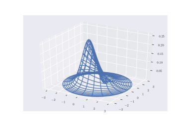
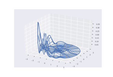
Figure 1. Peaks and valleys of some densities.

As a consequence, it is hardly feasible to simulate a DPP with more than one thousand points in a reasonable amount of time. As a DPP appears as the locations of the eigenvalues of some matrix ensembles, it may seem faster and simpler to draw random matrices and compute the eigenvalues with the optimized libraries to do so. There are several drawbacks to this approach: 1) we cannot control the domain into which the points fall, for some applications it may be important to simulate DPP restricted to some compact sets, 2) as eigenvalues belong to ${\mathbf{R}}$ or ${\mathbf{C}}$, we cannot imagine DPP in higher dimensions with this approach, 3) for stationary DPP, it is often useful to simulate under the Palm measure (see below) which is known to correspond to the distribution of the initial DPP with the first eigenvalue removed so no longer corresponds to a random matrix ensemble.

Several refinements of the algorithm 1 have been proposed along the years but the most advanced contributions have been made for DPP on lattices, which are of a totally different nature than continuous DPPs. We here propose to fasten the simulation of a DPP by reducing the number of eigenvalues considered and approximating the eigenfunctions by functions whose quadrature can be easily inversed to get rid of the rejection part.

We evaluate the impact of these approximations by bounding the distances between the original distribution of the DPP to be simulated and the real distribution according to which the points are drawn.

Actually, there are several notions of distances between the distributions of point processes (see [10] and references therein). We focus here on the total variation distance and on the quadratic Wasserstein distance. The former counts the difference of the number of points in an optimal coupling between two distributions. The latter evaluates the matching distance between two realizations of an optimal coupling provided that it exists.

The paper is organized as follows. We first recall the definition and salient properties of DPP. In Section 3, we briefly introduce the optimal transportation problem in its full generality and give some elements dedicated to point processes. In Section 4, we show how the eigenvalues and eigenfunctions do appear in the evaluation of the distances under scrutiny. In Section 5, we apply these results to the simulation of DPPs.

2. Determinantal point processes

Let $E$ be a Polish space, $\mathcal{O}(E)$ the family of all non-empty open subsets of $E$ and $\mathcal{B}$ denotes the corresponding Borel $\sigma$-algebra. In the sequel, $m$ is a Radon measure on $(E,\mathcal{B})$. Let ${\mathfrak{N}}$ be the space of locally finite subsets in $E$, also called the configuration space:

$${\mathfrak{N}}=\{\xi\subset E\,:\,|\Lambda\cap\xi|<\infty\,\text{ for any compact set }\Lambda\subset E\},$$

equipped with the topology of the vague convergence. We call elements of ${\mathfrak{N}}$ configurations and identify a locally finite configuration $\xi$ with the atomic Radon measure $\sum_{y\in\xi}\varepsilon_{y}$, where we have written $\varepsilon_{y}$ for the Dirac measure at $y\in E$.

Next, let ${\mathfrak{N}}^{f}=\{\xi\in{\mathfrak{N}}\,:\,|\xi|<\infty\}$ the space of all finite configurations on $E$. ${\mathfrak{N}}^{f}$ is naturally equipped with the trace $\sigma$-algebra $\mathcal{F}^{f}=\mathcal{F}|_{{\mathfrak{N}}^{f}}$.

A random point process is defined as a probability measure on $({\mathfrak{N}},\mathcal{F})$. A random point process $\mu$ is characterized by its Laplace transform, which is defined for any measurable non-negative function $f$ on $E$ as

$${\mathcal{L}}_{\mu}(f)=\int_{\mathfrak{N}}e^{-\sum_{x\in\xi}f(x)}\text{d}\mu(\xi).$$

Our notations are inspired by those of [14], where the reader can also find a brief summary of many properties of Papangelou intensities.

Definition 1.

We define the $m$-sample measure $L$ on $({\mathfrak{N}}^{f},\mathcal{F}^{f})$ by the identity

$$\int f(\alpha)\,\text{d}L(\alpha)=\sum_{n\geq 0}\frac{1}{n!}\int_{E^{n}}f(\{x_{1},\dots,x_{n}\})\text{d}m(x_{1})\ldots\text{d}m(x_{n}),$$

for any measurable nonnegative function $f$ on ${\mathfrak{N}}^{f}$.

Point processes are often characterized via their correlation function defined as:

Definition 2 (Correlation function).

A point process $\mu$ is said to have a correlation function $\rho:{\mathfrak{N}}^{f}\rightarrow{\mathbf{R}}$ if $\rho$ is measurable and

$$\int_{\mathfrak{N}}\sum_{\alpha\subset\xi,\ \alpha\in{\mathfrak{N}}^{f}}f(\alpha)\text{d}\mu(\xi)=\int_{{\mathfrak{N}}^{f}}f(\alpha)\,\rho(\alpha)\,\text{d}L(\alpha),$$

for all measurable nonnegative functions $f$ on ${\mathfrak{N}}^{f}$. For $\xi=\{x_{1},\dots,x_{n}\}$, we will write $\rho(\xi)=\rho_{n}(x_{1},\dots,x_{n})$ and call $\rho_{n}$ the $n$-th correlation function, where $\rho_{n}$ is a symmetrical function on $E^{n}$.

It can be noted that correlation functions can also be defined by the following property, both characterizations being equivalent in the case of simple point processes.

Definition 3.

A point process $\mu$ is said to have correlation functions $(\rho_{n},\,n\geq 0)$ if for any $A_{1},\dots,A_{n}$ disjoint bounded Borel subsets of $E$,

$$\mathbf{E}\left[{\prod_{i=1}^{n}\xi(A_{i})}\right]=\int_{A_{1}\times\dots\times A_{n}}\rho_{n}(x_{1},\dots,x_{n})\text{d}m(x_{1})\ldots\text{d}m(x_{n}).$$

Recall that $\rho_{1}$ is the mean density of particles with respect to $m$, and

$$\rho_{n}(x_{1},\dots,x_{n})\text{d}m(x_{1})\ldots\text{d}m(x_{n})$$

is the probability of finding a particle in the vicinity of each $x_{i}$, $i=1,\dots,n$.

Note that

$${\mathfrak{N}}_{E}^{f}=\bigcup_{n=0}^{\infty}{\mathfrak{N}}_{E}^{(n)}$$

where

$${\mathfrak{N}}_{E}^{(n)}=\{\xi\in{\mathfrak{N}}_{E}^{f},\,\xi(E)=n\}.$$

Since ${\mathfrak{N}}_{E}^{(n)}$ can be identified with $E^{n}/\mathfrak{S}_{n}$ where $\mathfrak{S}_{n}$ is the group of permutations over $n$ elements, every function $f\,:\,{\mathfrak{N}}_{E}^{f}\to{\mathbf{R}}$ is in fact equivalent to a family of symmetric functions $(f_{n},\,n\geq 1)$ where $f_{n}$ goes from $E^{n}$ to ${\mathbf{R}}$. For the sake of notations, we omit the index $n$ of $f_{n}$.

Definition 4.

A measure $\mu$ on ${\mathfrak{N}}_{E}^{f}$ is regular with respect to the reference measure $m$ when there exists

$$j\,:\,\bigcup_{n=0}^{\infty}{\mathfrak{N}}_{E}^{(n)} \longrightarrow{\mathbf{R}}^{+}$$

$$\{x_{1},\cdots,x_{n}\} \longmapsto j_{n}(x_{1},\cdots,x_{n})$$

where $j_{n}$ is symmetric on $E^{n}$ such that for any measurable bounded $f:{\mathfrak{N}}^{f}\rightarrow{\mathbf{R}}$,

(1) $$E[f(\xi)]=f(\emptyset)+\sum_{n=1}^{\infty}\frac{1}{n!}\int_{E^{n}}f(x_{1},\dots,x_{n})j(x_{1},\dots,x_{n})\text{d}m(x_{1})\dots\text{d}m(x_{n}).$$

The function $j_{n}$ is called the $n$-th Janossy density. Intuitively, it can be viewed as the probability to have exactly $n$ points in the vicinity $(x_{1},\cdots,x_{n})$

For details about the relationships between correlation functions and Janossy densities, see [7].

2.1. Determinantal point processes

For details, we mainly refer to [24]. A determinantal point on $X$ is characterized by a kernel $K$ and a reference measure $m$. The map $K$ is supposed to be an Hilbert-Schmidt operator from $L^{2}(E,\,m)$ into $L^{2}(E,\,m)$ which satisfies the following conditions:

1. $K$ is a bounded symmetric integral operator on $L^{2}(E,\,m)$, with kernel $K(.,.)$, i.e., for any $x\in E$,

   $$Kf(x)=\int_{E}{K(x,y)f(y)\text{d}m(y)}.$$

2. The spectrum of $K$ is included in $[0,\,1]$.

3. The map $K$ is locally of trace class, i.e., for all compact $\Lambda\subset E$, the restriction $K_{\Lambda}=P_{\Lambda}KP_{\Lambda}$ of $K$ to $L^{2}(\Lambda,\,m)$ is of trace class.

Definition 5.

The determinantal measure on ${\mathfrak{N}}$ with characteristics $K$ and $m$ can be defined through its correlation functions:

$$\rho_{n,\,K}(x_{1},\cdots,\,\,x_{n})=\det\bigl{(}K\left(x_{k},\,x_{l}\bigr{)}\right)_{1\leq k,l\leq n},$$

and for $n=0$, $\rho_{0,\,K}(\emptyset)=1$.

There is a particular class of DPP which is the basic blocks on which general DDP are built upon.

Definition 6.

A DPP whose spectrum is reduced to the singleton $\{1\}$ is called a projection DPP. Actually, its kernel is of the form

$$K_{\phi}(x,y)=\sum_{j=0}^{M}\phi_{j}(x)\phi_{j}(y)$$

where $M\in{\mathbf{N}}\cup\{\infty\}$ and $(\phi_{j},\,j=0,\cdots,M)$ is a family of orthonormal functions of $L^{2}(E,m)$.

If $M$ is finite then almost-all configurations of such a point process have $M$ atoms.

Alternatively, when the spectrum of $K$ does not contain $1$, we can define a DPP through its Janossy densities. In this situation, the properties of $K$ ensure that there exists a sequence $(\lambda_{i},\,i\geq 1)$ of elements of $[0,1)$ with no accumulation point but $0$ and a complete orthonormal basis $(\phi_{i},\,i\geq 1)$ of $L^{2}(m)$ such that

$$K_{\phi}(x,y)=\sum_{i\geq 1}\lambda_{i}\phi_{i}(x)\phi_{i}(y).$$

Note that if $L^{2}(E,\,m)$ is a ${\mathbf{C}}$-vector space, we must modify this definition accordingly:

$$K_{\phi}(x,y)=\sum_{i\geq 1}\lambda_{i}\phi_{i}(x)\overline{\phi_{i}(y)}.$$

For a compact subset $\Lambda\subset X$, the map $J_{\Lambda}$ is defined by:

$$J_{\Lambda}=\left(\operatorname{Id}-K_{\Lambda}\right)^{-1}K_{\Lambda},$$

so that we have:

$$\left(\operatorname{Id}-K_{\Lambda}\right)\left(\operatorname{Id}+J_{\Lambda}\right)=\operatorname{Id}.$$

For any compact $\Lambda\subset E,$ the operator $J_{\Lambda}$ is an Hilbert-Schmidt, trace class operator, whose spectrum is included in $[0,+\infty)$. We denote by $J_{\Lambda}$ its kernel. For any $n\in{\mathbf{N}}$, any compact $\Lambda\subset E$, and any $(x_{1},\cdots,\,x_{n})\in\Lambda^{n}$, the $n$-th Janossy density is given by:

(2) $$j_{\Lambda}^{n}\left(x_{1},\,\cdots,\,x_{n}\right)=\det\left(J_{\Lambda}\left(x_{k},\,x_{l}\right)\right)_{1\leq k,l\leq n}.$$

We can now state how the characteristics of a DPP are modified by some usual transformations on the configurations.

Theorem 1.

Let $\mu$ a DPP on ${\mathbf{R}}^{k}$ with kernel $K$ and reference measure $m=h\text{d}x$. Let $(\lambda_{n},\,n\geq 0)$ be its eigenvalues counted with multiplicity and $(\phi_{n},\,n\geq 0)$ the corresponds eigenfunctions.

1. A random thinning of probability $p$ transforms $\mu$ into a DPP of kernel $pK$.

2. A dilation of ratio $\rho$ transforms $\mu$ into a DPP of kernel

   $$K_{\rho}(x,y)=\frac{1}{\rho}\,K(\rho^{-1/k}x,\,\rho^{-1/k}y).$$

3. If $H$ is a $\mathcal{C}^{1}$-diffeomorphism on $E$, then

   $$\mathcal{H}\,:\,{\mathfrak{N}}_{E} \longrightarrow{\mathfrak{N}}_{E}$$

   $$\sum_{x\in\xi}\varepsilon_{x} \longrightarrow\sum_{x\in\xi}\varepsilon_{H(x)}$$

   transforms $\mu$ into a DPP of kernel

   $$K_{H}(x,y)=K\left(H^{-1}(x),\,H^{-1}(y)\right)$$

   and reference measure $m\circ H^{-1}$, the image measure of $m$ by $H$, see [6].

4. If $K(x,y)=k(x-y)$ then $\mu$ is stationary [20] and thus admits a stationary Palm measure $\mu^{0}$. From [24], we know that $\mu^{0}$ is distributed as the DPP of kernel

   $$K^{0}(x,y)=\sum_{n=1}^{\infty}\lambda_{n}\phi_{n}(x)\phi_{n}(y).$$

Remark 1.

It is straightforward to see that the spectrum of $K_{H}$ in $L^{2}(E,\,m\circ H^{-1})$ is the same as the spectrum of $K$ in $L^{2}(E,\,m)$. Actually, this transformation will be a particular case of the optimal maps obtained in solving the $\operatorname{MKP}$ for the Wassertein-2 distance (see Theorem 12).

Remark 2.

Recall that for a Poisson process, we can obtain a realization of its Palm measure by just adding an atom at $0$ to any of its realization. Unfortunately, we know from [18] that the eigenvalues of a DPP cannot be obtained as measurable functions of the configurations. Hence it is hopeless to construct a realization of $\mu^{0}$ from a realization of $\mu$.

2.1.1. Simulation of DPP

The simulation algorithm introduced [18] is up to now the most efficient to produce random configurations distributed according to a determinantal point process. It is based on the following lemma.

Lemma 2.

Let $\mu_{K,m}$ a determinantal point process of a trace-class kernel $K$ and reference measure $m$. Let $\operatorname{sp}(K;L^{2}(m))=\{\lambda_{n},i\geq 0\}$ and $(\phi_{n},\,i\geq 0)$ a CONB of $L^{2}(E,\,m)$ composed of eigenfunctions of $K$. Let $(B(\lambda_{n}),i\geq 0)$ a family of independent Bernoulli random variables of respective parameter $\lambda_{n}$. Let

$$I=\{n\geq 0,\,B(\lambda_{n})=1\}.$$

Since $\mathbf{E}\left[{|I|}\right]=\sum_{n=0}^{\infty}\lambda_{n}<\infty$, $I$ is a.s. a finite subset of ${\mathbf{N}}$. Consider

$$K_{I}(x,y)=\sum_{n\in I}\phi_{n}(x)\phi_{n}(y)$$

and

$$p_{I}(x_{1},\cdots,x_{|I|})=\frac{1}{|I|!}\det\Bigl{(}K_{I}(x_{k},x_{l}),\,1\leq k,l\leq|I|\Bigr{)}.$$

Construct a random configuration $\xi$ as follows: Given $I$, draw points $(W_{1},\cdots,W_{|I|})$ with joint density $p_{I}$. Then $\xi$ is distributed according to $\mu_{K,m}$.

In the following, let $\phi_{I}(x)=(\phi_{n}(x),n\in I)$.

Data: $R,I$

Result: $W_{1},\cdots,W_{|I|}$

Draw $W_{1}$ from the distribution with density $\|\phi_{I}(x)\|_{{\mathbf{C}}^{|I|}}^{2}/|I|$;

$e_{1}\leftarrow\phi_{I}(W_{1})/\|\phi_{I}(W_{1})\|_{{\mathbf{C}}^{|I|}}$;

for $i\leftarrow 2$ to $|I|$ do

      Draw $W_{i}$ from the distribution with density

$$p_{i}(x)=\frac{1}{|I|-i+1}\left(\left\|\phi_{I}(x)\right\|_{{\mathbf{C}}^{|I|}}^{2}-\sum_{k=1}^{i-1}|e_{k}.\phi_{I}(x)|^{2}\right)$$

$u_{i}\leftarrow\phi_{I}(W_{i})-\sum_{k=1}^{i-1}e_{k}.\phi_{I}(W_{i})\ e_{k}$;

       $e_{i}\leftarrow u_{i}/\|u_{i}\|_{{\mathbf{C}}^{|I|}}$;

      

end for

Algorithm 1 Sampling of the locations of the points given the set $I$ of active Bernoulli random variables.

We have two kind of difficulties here: the drawing of $W_{i}$ according to a density function with no particular feature so we usually have to resort to rejection sampling; when $|I|$ is large the computation of the density may be costly as it contains a sum of $|I|$ terms. Figure 1 also suggests that when the number of points becomes high, the profile of the conditional density might be very chaotic with high peaks and deep valleys, involving a large number of rejections in the sampling of this density. These are the problems we intend to address in the following.

Remark 3.

Note that this algorithm is fully applicable even if $E$ is a discrete finite space. It has been improved in several ways [19, 25] but when it comes to simulate a DPP with a large number of points as it is necessary in some applications [5], the best way remains to use MCMC methods [1]. Unfortunately, by its very construction, this last approach is not feasible when the underlying space $E$ is continuous.

3. Distances derived from optimal transport

For details on optimal transport in ${\mathbf{R}}^{d}$ and in general Polish spaces, we refer to [27, 26]. For $X$ and $Y$ two Polish spaces, for $\mu$ (respectively $\nu$) a probability measure on $X$ (respectively $Y$), $\Sigma(\mu,\,\nu)$ is the set of probability measures on $X\times Y$ whose first marginal is $\mu$ and second marginal is $\nu$. We also need to consider a lower semi continuous function $c$ from $X\times Y$ to ${\mathbf{R}}^{+}$. The Monge-Kantorovitch problem associated to $\mu$, $\nu$ and $c$, denoted by $\operatorname{MKP}(\mu$, $\nu$, $c$) for short, consists in finding

(3) $$\inf_{\gamma\in\Sigma(\mu,\,\nu)}\int_{X\times Y}c(x,y)\text{d}\gamma(x,\,y).$$

More precisely, since $X$ and $Y$ are Polish and $c$ is l.s.c., it is known from the general theory of optimal transportation, that there exists an optimal measure $\gamma\in\Sigma(\mu,\,\nu)$ and that the minimum coincides with

$$\sup_{(F,\,G)\in\Phi_{c}}(\int_{X}F\text{d}\mu+\int_{Y}G\text{d}\nu),$$

where $(F,\,G)$ are such that $F\in L^{1}(\text{d}\mu)$, $G\in L^{1}(\text{d}\nu)$ and $F(x)+G(y)\leq c(x,\,y)$. We will denote by ${\mathcal{W}}_{c}(\mu,\,\nu)$ the value of the infimum in (3). In the sequel, we need the following theorem of Brenier:

Theorem 3.

Let $c(x,y)=2^{-1}\|x-y\|^{2}$ be the Euclidean distance on ${\mathbf{R}}^{k}$ and $\mu,\,\nu$ two probability measures with finite second moment. If the measure $\mu$ is absolutely continuous with respect to the Lebesgue measure, there exists a unique optimal measure $\gamma_{{\text{opt}}}$ which realizes the minimum in (3). Moreover, there exists a unique function $\psi\,:\,{\mathbf{R}}^{k}\to{\mathbf{R}}$ such that

$$y=x-\nabla\psi(x),\ \gamma_{{\text{opt}}}\text{-a.s.}$$

Then, we have

$${\mathcal{W}}_{e}(\mu,\nu)=\frac{1}{2}\int_{{\mathbf{R}}^{k}}\|\nabla\psi\|_{{\mathbf{R}}^{k}}^{2}\text{d}\mu.$$

The square root of ${\mathcal{W}}_{e}(\mu,\nu)$ defines a distance on ${\mathfrak{M}}_{1}({\mathbf{R}}^{k})$, the set of probability measures on ${\mathbf{R}}^{k}$, called the Wasserstein-2 distance.

For $c$ a distance on $X=Y$, ${\mathcal{W}}_{c}$ also defines a distance on ${\mathfrak{M}}_{1}({\mathbf{R}}^{k})$, often called Kantorovitch-Rubinstein or Wasserstein-1 distance. It admits the alternative characterization.

Theorem 4 (See [11]).

Let $c$ be a distance on the Polish space $(X,d_{X})$. For $\mu$ and $\mu$ two probability measures on $X$,

$${\mathcal{W}}_{c}(\mu,\mu)=\sup_{f\in\operatorname{Lip}_{1}}\left(\int_{X}f\text{d}\mu-\int_{X}f\text{d}\nu\right)$$

where

$$\operatorname{Lip}_{1}=\left\{f\,:X\to{\mathbf{R}},\ \forall x,y\in X,|f(x)-f(y)|\leq d_{X}(x,y)\right\}.$$

Note that $d_{X}$ is the distance which defines the topology of the Polish space $X$, it may not be identical to $c$.

The next result is found in [26, Chapter 7].

Theorem 5.

The topologies induced by ${\mathcal{W}}_{c}$ and ${\mathcal{W}}_{e}$ on ${\mathfrak{M}}_{1}({\mathbf{R}}^{k})$ are strictly stronger than the topology of convergence in distribution.

4. Distances between point processes

There are several ways to define a distance between point processes. We here focus on two of them. They are constructed similarly: Choose a cost function $c$ on ${\mathfrak{N}}_{E}$ and then consider ${\mathcal{W}}_{c}$ defined by the solution of $\operatorname{MKP}(\mu,\nu,c)$ for $\mu$ and $\nu$ two elements of ${\mathfrak{M}}_{1}({\mathfrak{N}}_{E})$.

Definition 7.

Consider $\operatorname{dist}_{\text{\small{TV}}}$ the distance in total variation between two configurations (viewed as discrete measures):

$$\operatorname{dist}_{\text{\small{TV}}}(\xi,\zeta)=(\xi\Delta\zeta)(E)$$

where $\xi\Delta\zeta$ is the symmetric difference between the two sets $\xi$ and $\zeta$, i.e. we count the number of distinct atoms between $\xi$ and $\zeta$. Then, for $\mu$ and $\nu$ belonging to ${\mathfrak{M}}_{1}({\mathfrak{N}}_{E})$, their Kantorovitch-Rubinstein distance is defined by

$${\mathcal{W}}_{\text{\small{KR}}}(\mu,\nu) =\inf_{\begin{subarray}{c}\text{law}(\xi)=\mu\\ \text{law}(\zeta)=\nu\end{subarray}}\mathbf{E}\left[{(\xi\Delta\zeta)(E)}\right]$$

(4) $$=\sup_{f\in\operatorname{Lip}_{1}({\mathfrak{N}}_{E})}\left(\int_{{\mathfrak{N}}_{E}}f(\xi)\text{d}\mu(\xi)-\int_{{\mathfrak{N}}_{E}}f(\zeta)\text{d}\nu(\zeta)\right).$$

Remark 4.

For any compact set $\Lambda\subset E$, the map

$$\Xi_{\Lambda}\,:\,{\mathfrak{N}}_{E} \longrightarrow{\mathbf{N}}$$

$$\xi \longmapsto\xi(\Lambda)$$

is Lipschitz. Let $(\mu_{n},\,n\geq 1)$ be a sequence of point processes and denote by $\xi_{n}$ an ${\mathfrak{N}}_{E}$-valued random variable whose distribution is $\mu_{n}$. Similarly, for another element $\nu\in{\mathfrak{M}}_{1}({\mathfrak{N}}_{E})$, let $\zeta$ be an ${\mathfrak{N}}_{E}$-valued random variable whose distribution is $\nu$. In view of (4) and Theorem 4, if ${\mathcal{W}}_{\text{\small{KR}}}(\mu_{n},\nu)$ tends to zero then for any compact set $\Lambda$, the sequence of random variables $(\xi_{n}(\Lambda),\,n\geq 1)$ converges in distribution to $\zeta(\Lambda)$.

For the quadratic distance, we first consider, on $E={\mathbf{R}}^{k}$, the cost function as $\rho(x,y)=2^{-1}\|x-y\|^{2}$ and we define a cost between configurations (see also [4, 3, 2]) as the ’lifting’ of $\rho$ on ${\mathfrak{N}}_{E}$:

$$c(\xi_{1},\xi_{2})=\inf\left\{\int\rho(x,y)\ \text{d}\beta(x,y),\ \beta\in\Sigma({\xi_{1},\xi_{2}})\right\},$$

where $\Sigma({\xi_{1},\xi_{2}})$ denotes the set of $\beta\in{\mathfrak{N}}_{E\times E}$ having marginals $\xi_{1}$ and $\xi_{2}.$ First remark that when $\xi_{1}(E)$ is finite, the cost is finite only if $\xi_{1}(E)=\xi_{2}(E)$, otherwise $\Sigma({\xi_{1},\xi_{2}})$ is empty and then, by convention, the cost is infinite. Moreover, the cost is attained at the permutation of $\{1,\cdots,\xi_{1}(E)\}$ which minimizes the sum of the squared distances:

$$c(\xi_{1},\xi_{2})=\frac{1}{2}\min_{\sigma\in\mathfrak{S}_{\xi_{1}(E)}}\sum_{j=1}^{\xi_{1}(E)}\|x_{i}-y_{\sigma(i)}\|^{2}$$

where $\xi_{1}=\{x_{j},1\leq j\leq\xi_{1}(E)\}$ and $\xi_{2}=\{y_{j},1\leq j\leq\xi_{1}(E)\}$. For infinite configurations, it is not immediate that the cost function so defined has the minimum regularity required to consider an optimal transport problem. According to [23], this is indeed true as $c$ is lower semi continuous on ${\mathfrak{N}}_{E}\times{\mathfrak{N}}_{E}$. We can then consider the Monge-Kantorovitch problem $\operatorname{MKP}(\mu,\nu,c)$ on ${\mathfrak{M}}_{1}({\mathfrak{N}}_{E})$. The main theorem of [8] is the following. For $\Lambda$ a compact subset of $E$, by definition of locally finite point process, the number of points of $\xi_{|\Lambda}$ is finite hence we can write

$${\mathfrak{N}}_{\Lambda}=\bigcup_{n=0}^{\infty}{\mathfrak{N}}_{\Lambda}^{(n)}$$

where

$${\mathfrak{N}}_{\Lambda}^{(n)}=\left\{\xi\in{\mathfrak{N}}_{\Lambda},\ \xi(\Lambda)=n\right\}.$$

Definition 8.

A probability measure $\mu$ on ${\mathfrak{N}}_{E}$ is said to be regular whenever it admits Janossy densities of any order.

Theorem 6.

Let $\Lambda\subset E$ a compact set. Let $\mu$ be a regular probability measure on ${\mathfrak{N}}_{\Lambda}$ and $\nu$ be a probability measure on ${\mathfrak{N}}_{E}$. The Monge-Kantorovitch distance, associated to $c$, between $\mu$ and $\nu$ is finite if and only if the following two conditions hold

1. $\mu(\zeta(\Lambda)=n)=\nu(\xi(E)=n):={\mathfrak{c}}_{n}$ for any integer $n\geq 0$,

2. $\sum_{n\geq 1}{\mathfrak{c}}_{n}\,{\mathcal{W}}_{e}(\mu_{n},\,\nu_{n})$ is finite.

Then, the solution of $\operatorname{MKP}(\mu,\nu,c)$ is attained at a unique point $\gamma_{{\text{opt}}}$ and there exists a unique map

$$\varphi\,:\,\bigcup_{n=0}^{\infty}{\mathfrak{N}}_{\Lambda}^{(n)} \longrightarrow\bigcup_{n=0}^{\infty}{\mathfrak{N}}_{E}^{(n)}$$

$$\xi=\{x_{1},\cdots,x_{n}\} \longmapsto\{\varphi_{n}\bigl{(}y;\,(x_{1},\cdots,x_{n})\bigr{)},\ y\in\xi\}\in E^{n}$$

such that for $\xi\in{\mathfrak{N}}_{\Lambda}^{(n)},$

$$\zeta=\sum_{x\in\xi}\varepsilon_{\varphi_{n}(x,\,\xi)},\gamma_{{\text{opt}}}\text{-a.s.}$$

Moreover,

(5) $${\mathcal{W}}_{c}(\mu,\,\nu)=\sum_{n\geq 1}{\mathfrak{c}}_{n}{\mathcal{W}}_{e}(\mu_{n},\,\nu_{n}).$$

If $\nu$ is regular, then for $y\in\{x_{1},\cdots,x_{n}\}$,

$$\varphi_{n}(y,(x_{1},\cdots,x_{n}))=y-\nabla_{y}\psi_{n}(x_{1},\cdots,x_{n})$$

where $\operatorname{Id}-\nabla\psi_{n}$ is the optimal transportation map between the $n$-th Janossy normalized densities ${\mathfrak{c}}_{n}^{-1}\,j_{n}^{\mu}$ and ${\mathfrak{c}}_{n}^{-1}\,j_{n}^{\nu}$.

This means that whenever the distance between $\mu$ and $\nu$ is finite, there exists a strong coupling which works as follows: 1) draw a discrete random variable with the distribution of $\xi(\Lambda)$, let $\iota$ the obtained value 2) draw the points of $\xi$ according to $\mu_{\iota}$ and then 3) apply the map $\varphi_{\iota}(.,\,\xi)$ to each point of $\xi$. The configuration which is obtained is distributed according to $\nu_{\iota}$.

It is shown in [8] that for two Poisson point processes of respective intensity $\sigma_{1}$ and $\sigma_{2}$, the distance defined above is finite if and only if $\sigma_{1}(E)=\sigma_{2}$ and

$$\zeta=\sum_{x\in\xi}\varepsilon_{t(x)},\ \gamma_{{\text{opt}}}\text{-a.s.}$$

where $t$ is the optimal transport map between $\sigma_{1}$ and $\sigma_{2}$ for the Euclidean cost as defined in Theorem 3. Note that the optimal map is a transformation which is applied to each atom irrespectively of the others. In full generality, for non Poisson processes, the amount by which an atom is moved depends on the other locations.

4.1. Distances between DPP

For determinantal point processes, we can evaluate the effect of a modification of the eigenvalues with the Kantorovitch-Rubinstein distance and the effect of a modification of the eigenvectors with the Wasserstein-2 distance.

Lemma 7.

Let $\mu$ and $\nu$ two determinantal point processes with respective kernels $K_{\mu}$ and $K_{\nu}$. Assume that $K_{\mu}$ and $K_{\nu}$ are two projection kernels in some Hilbert space $L^{2}(m)$ such that $K_{\mu}=K_{\nu}+L$ where $L$ is another projection kernel and $L$ is orthogonal to $K_{\nu}$. Then,

(6) $${\mathcal{W}}_{\text{\small{KR}}}(\mu,\,\nu)\leq\text{range}(L).$$

Proof.

The hypothesis means that there exists $(\phi_{j},\,j=1,\cdots,l+n)$ a family of orthonormal functions in $L^{2}(m)$ such that

$$K_{\nu}(x,y)=\sum_{j=1}^{n}\phi_{j}(x)\phi_{j}(y)\text{ and }L(x,y)=\sum_{j=n+1}^{l}\phi_{j}(x)\phi_{j}(y).$$

Since $L$ is a positive symmetric operator, this exactly means that $K_{\nu}\prec K_{\mu}$ in the Loewner sense. According to [15], there exists $\xi^{\prime},\,\zeta^{\prime}$ of respective distribution $\mu$, $\nu$ and a point process $\omega^{\prime}$ such that

$$\xi^{\prime}=\zeta^{\prime}+\omega^{\prime}\text{ and }\zeta^{\prime}\cap\omega^{\prime}=\emptyset.$$

This implies that

$$\xi^{\prime}\Delta\zeta^{\prime}(E)=\omega^{\prime}(E)=l.$$

According to the first definition of ${\mathcal{W}}_{\text{\small{KR}}}$, see (4), this implies (6). ∎

Theorem 8.

Let $\mu$ (respectively $\nu$) be a determinantal point process of characteristics $K_{\mu}$ and $h_{\mu}$ (respectively $K_{\nu}$ and $h_{\nu}$) on a compact set $\Lambda\subset{\mathbf{R}}^{k}$. Denote by $(\lambda_{n}^{\mu},\,n\geq 0)$ (respectively $(\lambda_{n}^{\nu},\,n\geq 0)$) the eigenvalues of $K_{\mu}$ in $L^{2}(E,\,h_{\mu}\text{d}x)$ (respectively of $K_{\nu}$ in $L^{2}(E,\,h_{\nu}\text{d}x)$) counted with multiplicity and ranked in decreasing order. Assume that

$$\lambda_{n}^{\nu}\leq\lambda_{n}^{\mu},\ \forall n\geq 0.$$

Then,

(7) $${\mathcal{W}}_{\text{\small{KR}}}(\mu,\,\nu)\leq\sum_{n=0}^{\infty}|\lambda_{n}^{\mu}-\lambda_{n}^{\nu}|.$$

Proof.

We make a coupling of $(B(\lambda_{n}^{\mu}),\,n\geq 0)$ and $(B(\lambda_{n}^{\mu}),\,n\geq 0)$ by using the same sequence of uniform random variables: Let $(U_{n},\,n\geq 0)$ be a sequence of independent, identically uniformly distributed over $[0,1]$, random variables, consider

$$X^{\mu}_{n}=\mathbf{1}_{\{U_{n}\leq\lambda_{n}^{\mu}\}}\text{ and }X_{n}^{\nu}=\mathbf{1}_{\{U_{n}\leq\lambda_{n}^{\nu}\}}.$$

Note that

(8) $$\mathbf{P}(X_{n}^{\nu}\neq X_{n}^{\mu})=|\lambda_{n}^{\mu}-\lambda_{n}^{\nu}|.$$

Let $I_{\mu}=\{n\geq 0,X_{n}^{\mu}=1\}$ and $I_{\nu}=\{n\geq 0,X_{n}^{\nu}=1\}$. In view of the hypothesis, $X^{\nu}\leq X^{\mu}$ hence $I_{\nu}\subset I_{\mu}$. Otherwise stated, $K_{I_{\mu}}$ and $K_{I_{\nu}}$ are two projection kernels which satisfy the hypothesis of Lemma 7. Hence, there exists a realization $(\xi,\zeta)$ of $\Sigma(\mu,\nu)$ given $I_{\mu}$ and $I_{\nu}$, such that

$$\operatorname{dist}_{\text{\small{TV}}}(\xi,\,\zeta)={\sum_{n=0}^{\infty}\mathbf{1}_{\{X_{n}^{\nu}\neq X_{n}^{\mu}\}}}.$$

Gluing these realizations together, we get a coupling $(\xi,\zeta)$ such that

$$\mathbf{E}\left[{\operatorname{dist}_{\text{\small{TV}}}(\xi,\,\zeta)}\right] =\mathbf{E}\left[{\mathbf{E}\left[{\operatorname{dist}_{\text{\small{TV}}}(\xi,\,\zeta)\,|\,I_{\mu},I_{\nu}}\right]}\right]$$

$$=\mathbf{E}\left[{\sum_{n=0}^{\infty}\mathbf{1}_{\{X_{n}^{\nu}\neq X_{n}^{\mu}\}}}\right]$$

$$=\sum_{n=0}^{\infty}|\lambda_{n}^{\mu}-\lambda_{n}^{\nu}|,$$

according to (8). Since the Kantorovitch-Rubinstein distance is obtained as the infimum over all couplings of the total variation distance between $\xi$ and $\zeta$, this particular construction shows that (7) holds. ∎

The next corollary is an immediate consequence of the alternative definition of the KR distance on point processes, see Eqn. (4).

Corollary 9.

With the hypothesis of Theorem 8, let $\xi$ and $\zeta$ be random point process of respective distribution $\mu$ and $\nu$. Then, we have that

$$\sup_{A\subset\Lambda}\operatorname{dist}_{\text{\small{TV}}}(\xi(A),\,\zeta(A))\leq\sum_{n=0}^{\infty}|\lambda_{n}^{\mu}-\lambda_{n}^{\nu}|.$$

This means that the Kantorovitch-Rubinstein distance between point processes focuses on the number of atoms in any compact. As we shall see now, the Wasserstein-2 distance evaluates the matching distance between configurations when they have the same cardinality.

Theorem 10.

Let $\mu$ (respectively $\nu$) be a determinantal point process of characteristics $K_{\mu}$ and $h_{\mu}$ (respectively $K_{\nu}$ and $h_{\nu}$) on a compact set $\Lambda\subset{\mathbf{R}}^{k}$. The Wasserstein-2 distance between $\mu$ and $\nu$ is finite if and only if

$$\text{sp}(K_{\mu};\,L^{2}(h_{\mu}\!\text{d}x))=\text{sp}(K_{\nu};\,L^{2}(h_{\nu}\!\text{d}x)).$$

Proof of Theorem 10.

According to point 1 of Theorem 6, we must first prove the equality of the spectra. We already know that the eigenvalues of both kernels are between $0$ and $1$, with no other accumulation point than $0$. Furthermore, the distribution of $\zeta(\Lambda)$ is that of the sum of independent Bernoulli random variables of parameters given by the eigenvalues, hence

(9) $$\Phi_{\mu}(z)=\mathbf{E}_{\mu}\left[{z^{\zeta(\Lambda)}}\right]=\prod_{\lambda\in\operatorname{sp}K_{\mu}}(1-\lambda+\lambda z).$$

The infinite product is convergent since $\operatorname{trace}K_{\mu}=\sum_{\lambda\in\operatorname{sp}K_{\mu}}$ is finite.

If the Wasserstein-2 distance between $\mu$ and $\nu$ is finite then $\Phi_{\mu}=\Phi_{\nu}$. The zeros of these two holomorphic functions are all greater than $1$ and are isolated. Let

$$m(\Phi,r)=\text{number of zeros (counted with multiplicity) of $\Phi$ in $B(0,\,r)$}.$$

By the properties of zeros of holomorphic functions we have

$$m(\Phi_{\mu},r)=m(\Phi_{\nu},r)\text{ for any }r\geq 0.$$

Hence,

$$\Big{\{}\frac{1-\lambda}{\lambda},\ \lambda\in\operatorname{sp}K_{\mu}\Big{\}}=\Big{\{}\frac{1-\lambda}{\lambda},\ \lambda\in\operatorname{sp}K_{\nu}\Big{\}}$$

and the two spectra must coincide. Now then, by the very definition of ${\mathcal{W}}_{e}$,

$${\mathcal{W}}_{e}(\mu_{n},\nu_{n})\leq\int_{\Lambda}\|x\|^{2}(\text{d}\mu_{n}+\text{d}\nu_{n})\leq\sup_{x\in\Lambda}\|x\|^{2}\Bigl{(}\mu_{n}(\Lambda)+\nu_{n}(\Lambda)\Bigr{)}.$$

Thus, we have

$$\sum_{n\geq 1}{\mathcal{W}}_{e}(\mu_{n},\,\nu_{n})\ \mu(\zeta(\Lambda)=n)\leq\sup_{x\in\Lambda}\|x\|^{2}\sum_{n\geq 1}\Bigl{(}\mu_{n}(\Lambda)+\nu_{n}(\Lambda)\Bigr{)}\mu(\zeta(\Lambda)=n)\\ =2\sup_{x\in\Lambda}\|x\|^{2}\operatorname{trace}K_{\mu}.$$

This quantity is finite hence the Wasserstein-2 distance between $\mu$ and $\nu$ as soon as the spectra are equal. ∎

The next lemma is a straightforward consequence of Lemma 2.

Lemma 11.

Let $\mu$ be a determinantal point process of characteristics $K_{\mu}$ and $h_{\mu}$. For $I$ a finite subset, let

$$c_{I}=\prod_{i\in I}\lambda_{i}^{\mu}\,\prod_{j\in I^{c}}(1-\lambda_{j}^{\mu}),$$

where the $\lambda^{\mu}_{i}$’s are the eigenvalues of $K_{\mu}$. Then, its $n$-th Janossy density is given by

$$j_{n}^{\mu}(x_{1},\cdots,x_{n})=\sum_{\begin{subarray}{c}I\subset{\mathbf{N}}\\ |I|=n\end{subarray}}c_{I}\,p_{I}(x_{1},\cdots,x_{n}).$$

This means that given $\zeta(E)=n$, the points are distributed according to the probability measure:

$${\mathfrak{p}}^{\mu}_{n}\,:\,(x_{1},\cdots,x_{n})\longmapsto{\mathfrak{c}}_{n}^{-1}\sum_{\begin{subarray}{c}I\subset{\mathbf{N}}\\ |I|=n\end{subarray}}c_{I}\,p_{I}(x_{1},\cdots,x_{n})\text{ where }{\mathfrak{c}}_{n}=\sum_{\begin{subarray}{c}I\subset{\mathbf{N}}\\ |I|=n\end{subarray}}c_{I}.$$

Proof.

Consider that $\xi$ is constructed with Algorithm 1 and denote by $I_{\xi}$ the set of indices of the Bernoulli random variables which are equal to $1$ for the drawing of $\xi$. For any bounded $f\,:\,{\mathfrak{N}}^{f}_{E}\to{\mathbf{R}}$,

$$\mathbf{E}\left[{f(\xi)}\right] =f(\emptyset)+\sum_{n=1}^{\infty}\mathbf{E}\left[{f(\xi)\mathbf{1}_{\{\xi(E)=n\}}}\right]$$

$$=f(\emptyset)+\sum_{n=1}^{\infty}\sum_{\begin{subarray}{c}J\subset{\mathbf{N}}\\ |J|=n\end{subarray}}\mathbf{E}\left[{f(\xi)\,|\,{I_{\xi}=J}}\right]\,c_{J}$$

$$=f(\emptyset)+\sum_{n=1}^{\infty}\sum_{\begin{subarray}{c}J\subset{\mathbf{N}}\\ |J|=n\end{subarray}}c_{J}\int_{E^{n}}f(x_{1},\cdots,x_{n})\,p_{J}(x_{1},\cdots,x_{n})\text{d}x_{1}\ldots\text{d}x_{n}$$

$$=f(\emptyset)+\sum_{n=1}^{\infty}{\mathfrak{c}}_{n}\int_{E^{n}}f(x_{1},\cdots,x_{n})\,{\mathfrak{p}}_{n}^{\mu}(x_{1},\cdots,x_{n})\text{d}x_{1}\ldots\text{d}x_{n}.$$

The result follows by identification with (1). ∎

Then, Theorem 6 applies as follows.

Theorem 12.

Suppose that the hypothesis of Theorem 10 hold. Let $\operatorname{Id}-\nabla\psi_{n}$ be the optimal transport map between ${\mathfrak{p}}^{\mu}_{n}$ and ${\mathfrak{p}}^{\nu}_{n}$. Then, the optimal coupling is given by the following rule: For $\xi$ such that $\xi(E)=n$, it is coupled with $\zeta$ the configuration with $n$ atoms described by

$$\zeta=\sum_{x\in\xi}\varepsilon_{x-\nabla_{x}\psi_{n}(\xi)}.$$

Furthermore,

$${\mathcal{W}}_{c}(\mu,\nu) =\sum_{n=1}^{\infty}{\mathfrak{c}}_{n}\,{\mathcal{W}}_{e}({\mathfrak{p}}_{n}^{\mu},\,{\mathfrak{p}}_{n}^{\nu})$$

$$=\frac{1}{2}\sum_{n=1}^{\infty}\int_{E^{n}}\|\nabla\psi_{n}(x_{1},\cdots,x_{n})\|^{2}_{E^{n}}\ j_{n}^{\mu}(x_{1},\cdots,x_{n})\text{d}x_{1}\ldots\text{d}x_{n}.$$

Theorems 10 and 12 mean that two determinantal point processes are strongly coupled when and only when their eigenvalues are identical. Moreover, the eigenvalues also control the convex combination of the densities of the projection DPP which appear in the Janossy densities.

4.2. Determinantal projection processes

Recall from Definition 6 that a projection DPP has a spectrum reduced to $\{1\}$. When it is of finite rank $M$, almost all its configurations have $M$ points distributed according to the density

(10) $$p_{\phi}(x_{1},\cdots,x_{M})=\frac{1}{M!}\det\Bigl{(}K_{\phi}(x_{i},\,x_{j}),\,1\leq i,j\leq M\Bigr{)}.$$

Theorem 12 cannot be used as is since projection DPPs do not possess Janossy densities. However, the initial definition of ${\mathcal{W}}_{c}$ can still be used.

Theorem 13.

Let $\psi=(\psi_{j},\,1\leq j\leq M)$ and $\psi=(\psi_{j},\,1\leq j\leq M)$ two orthonormal families of $L^{2}(E;m)$. Let $\mu_{\psi}$ and $\mu_{\phi}$ the two projection DPP associated to these families. Then,

$${\mathcal{W}}_{c}(\mu_{\psi},\,\mu_{\phi})\leq\inf_{\sigma\in\mathfrak{S}_{M}}\sum_{j=1}^{M}{\mathcal{W}}_{e}(|\psi_{j}|^{2}\text{d}m,\,|\phi_{\sigma(j)}|^{2}\text{d}m).$$

Proof.

We know that the points of $\mu_{\psi}$ (respectively $\mu_{\phi}$) are distributed according to $p_{\psi}$ (respectively $p_{\phi}$) given by (10). Let $\gamma$ be a probability measure on $E^{M}\times E^{M}$ whose marginals are $p_{\psi}\text{d}m$ and $p_{\phi}\text{d}m$. We know that

$${\mathcal{W}}_{c}(\mu_{\psi},\,\mu_{\phi}) =\int_{E^{M}\times E^{M}}\inf_{\sigma\in\mathfrak{S}_{M}}\sum_{j=1}^{M}|x_{j}-y_{\sigma(j)}|_{E}^{2}\ \text{d}\gamma(x_{1},\cdots,x_{M},y_{1},\cdots,y_{M})$$

$$\leq\sum_{j=1}^{M}\int_{E^{M}\times E^{M}}|x_{j}-y_{j}|_{E}^{2}\ \text{d}\gamma(x_{1},\cdots,x_{M},y_{1},\cdots,y_{M}).$$

We know from Algorithm 1, that the marginal distribution a single atom of $\mu_{\psi}$ has distribution

$$\text{d}\mu_{\psi}^{1}(x)=\frac{1}{M}\sum_{j=1}^{M}|\psi_{j}(x)|^{2}\text{d}m(x).$$

Since $p_{\psi}$ and $p_{\phi}$ are both invariant with respect to permutations, we obtain

$${\mathcal{W}}_{c}(\mu_{\psi},\,\mu_{\phi}) \leq M\ \int_{E\times E}|x_{1}-y_{1}|_{E}^{2}\text{d}\gamma(x_{1},\cdots,x_{M},y_{1},\cdots,y_{M})$$

$$\leq M\ {\mathcal{W}}_{e}(\mu_{\psi}^{1},\mu_{\phi}^{1}).$$

If $\gamma_{i}^{1}$ is a coupling between $|\psi_{i}|^{2}\text{d}m$ and $|\phi_{i}|^{2}\text{d}m$ then $M^{-1}\sum_{i=1}^{M}\gamma_{i}^{1}$ is a coupling between $\mu_{\psi}^{1}$ and $\mu_{\phi}^{1}$. Hence,

$${\mathcal{W}}_{c}(\mu_{\psi},\,\mu_{\phi}) \leq\sum_{j=1}^{M}\int_{E\times E}|x_{1}-y_{1}|^{2}\text{d}\gamma^{1}_{j}(x_{1},y_{1})$$

$$\leq\sum_{j=1}^{M}{\mathcal{W}}_{e}(|\psi_{j}|^{2}\text{d}m,|\phi_{j}|^{2}\text{d}m).$$

Since we can order the elements of the family $\psi$ and $\phi$ in any order, the result follows. ∎

5. Simulation

As mentioned previously, implementing Algorithm 1 using rejection sampling involves too many rejections which prevents the algorithm to work for more than $1\,000$ points. In this section, we will show that we can generate $10\,000$ points for the Ginibre point process on a compact disc using inverse transform sampling and approximation of the kernel.

In this section, we will consider Ginibre point processes but our reasoning could be applied to any rotational invariant determinantal process like the polyanalytic ensembles [16, 13] or the Bergman process [17]. For these processes, it is relatively easy to compute the eigenvalues and the eigenfunctions of the kernel of their restriction to a ball centered at the origin. For the Ginibre process, which will be our toy model, its restriction to $\mathcal{B}_{R}$, denoted by $\mathfrak{G}^{R}$, has a kernel of the form

$$K^{R}_{N}(x,y)=\sum_{n=0}^{\infty}\lambda_{n}^{R}\phi_{n}^{R}(x)\overline{\phi_{n}^{R}(y)}$$

where [9]

$$\lambda_{n}^{R} =\frac{\gamma(n+1,R^{2})}{n!}$$

$$\phi_{n}^{R}(x) =\frac{1}{\sqrt{\pi\gamma(n+1,R^{2})}}\ x^{n}e^{-|x|^{2}/2},$$

with $\gamma(n,r)$ is the lower incomplete gamma function. We denote by the $\mathfrak{G}^{R}_{N}$ the process whose kernel is the truncation of $K_{R}$ to its first $N$ components:

$$K^{R}_{N}(x,y)=\sum_{n=0}^{N-1}\lambda_{n}^{R}\phi_{n}^{R}(x)\overline{\phi_{n}^{R}(y)}$$

The strict application of Algorithm 1 for the simulation of $\mathfrak{G}^{R}$, requires to compute all the quantities of the form

$$\lambda_{n}^{R}\prod_{k=n+1}^{\infty}(1-\lambda_{k}^{R})$$

to determine which Bernoulli random variables are active. Strictly speaking, this is unfeasible. However, it is a well known observation that the number of points of $\mathfrak{G}^{R}$ is about $R^{2}$. So it is likely that $\mathfrak{G}^{R}$ and $\mathfrak{G}^{R}_{N_{R}}$ should be close for $N_{R}$ close to $R^{2}$. This is what proves the next theorem.

Theorem 14.

Let $c>0$ and $N_{R}=(R+c)^{2}$. For $R>c$, we have

$${\mathcal{W}}_{\text{\small{KR}}}(\mathfrak{G}^{R},\,\mathfrak{G}^{R}_{N_{R}})\leq\sqrt{\frac{2}{\pi}}Re^{-c^{2}}.$$

Actually, the proof says that with high probability, $\mathfrak{G}^{R}$ and $\mathfrak{G}_{N_{R}}^{R}$ do coincide.

Proof.

First, using the integral expression $\gamma(j,x)=\int_{t=0}^{x}t^{j-1}e^{-t}dt$, observe that $\sum_{j=1}^{\infty}\frac{\gamma(j,x)}{\Gamma(j)}=x$. Then, using the formula $\gamma(n+1,x)=n\gamma(n,x)-x^{n}e^{-x}$, we have by induction:

$$\sum_{j=n+1}^{\infty}\frac{\gamma(j,x)}{\Gamma(j)}=\frac{x^{n}e^{-x}-(n-x)\gamma(n,x)}{\Gamma(n)}\cdotp$$

For $n=(R+c)^{2}$ and $x=R^{2}$, this implies:

$$\sum_{j\geq(R+c)^{2}}\lambda_{j}^{R} \leq(R+c)^{2}\frac{R^{2(R+c)^{2}}e^{-R^{2}}}{(R+c)^{2}!}$$

Using the bound $n!\geq\sqrt{2\pi n}\left(\frac{n}{e}\right)^{n}$

$$\sum_{j\geq(R+c)^{2}}\lambda_{j}^{R} \leq\frac{R+c}{\sqrt{2\pi}}\frac{R^{2(R+c)^{2}}e^{(R+c)^{2}-R^{2}}}{(R+c)^{2(R+c)^{2}}}$$

$$\leq\frac{R+c}{\sqrt{2\pi}}e^{(R+c)^{2}-R^{2}-2(R+c)^{2}\log(1+\frac{c}{R})}$$

$$\leq\frac{R+c}{\sqrt{2\pi}}e^{(R+c)^{2}-R^{2}-2(R+c)^{2}\frac{\frac{c}{R}}{1+\frac{c}{R}}}$$

$$\leq\frac{R+c}{\sqrt{2\pi}}e^{-c^{2}}$$

Since $R>c$, the proof is complete. ∎

As a corollary of the previous proof, we have

(11) $$\mathbf{P}(\exists n\geq(R+c)^{2},\text{Ber}(\lambda_{n}^{R})=1)\leq\sum_{n\geq(R+c)^{2}}\lambda_{n}^{R}\leq\kappa Re^{{-c^{2}}}$$

for $R$ large enough. This means that the number of active Bernoulli random variables in Algorithm 1 is less than $(R+c)^{2}$ with high probability. We can also provide a lower bound on the cardinality of $I$.

Lemma 15.

For any $R>c>0$,

$$\mathbf{P}(\text{card}(I)<(R-c)^{2})\leq\frac{1}{\sqrt{2\pi}}Re^{-c^{2}}.$$

Proof.

As in the previous proof, we will reduce the problem to bound a sum of reduced incomplete gamma functions.

$$\mathbf{P}(\text{card}(I)<(R-c)^{2}) =1-\mathbf{P}(\text{card}(I)\geq(R-c)^{2})$$

$$\leq 1-\prod_{0\leq j<\lfloor{(R-c)^{2}}\rfloor}\mathbf{P}(Ber(\lambda_{j}^{R})=1)$$

$$\leq\sum_{0\leq j<\lfloor{(R-c)^{2}}\rfloor}(1-\mathbf{P}(Ber(\lambda_{j}^{R})=1))$$

$$\leq\sum_{1\leq j\leq\lfloor{(R-c)^{2}}\rfloor}\frac{\Gamma(j,R^{2})}{\Gamma(j)}\cdotp$$

Using the formula $\Gamma(n+1,x)=n\Gamma(n,x)+x^{n}e^{-x}$, we have by induction:

$$\sum_{j=1}^{n}\frac{\Gamma(j,x)}{\Gamma(j)}=\frac{x^{n}e^{-x}-(x-n)\Gamma(n,x)}{\Gamma(n)}\cdotp$$

For $n=\lfloor{(R-c)^{2}}\rfloor$ and $x=R^{2}$, this implies:

$$\mathbf{P}(\text{card}(I)<(R-c)^{2}) \leq(R-c)^{2}\frac{R^{2(R-c)^{2}}e^{-R^{2}}}{(R-c)^{2}!}\cdotp$$

Using Stirling formula

$$\mathbf{P}(\text{card}(I)<(R-c)^{2}) \leq\frac{R-c}{\sqrt{2\pi}}\frac{R^{2(R-c)^{2}}e^{(R-c)^{2}-R^{2}}}{(R-c)^{2(R-c)^{2}}}$$

$$\leq\frac{R-c}{\sqrt{2\pi}}e^{(R-c)^{2}-R^{2}-2(R-c)^{2}\log(1-\frac{c}{R})}$$

$$\leq\frac{R-c}{\sqrt{2\pi}}e^{(R-c)^{2}-R^{2}+2(R-c)^{2}\frac{\frac{c}{R}}{1-\frac{c}{R}}}$$

$$\leq\frac{R-c}{\sqrt{2\pi}}e^{-c^{2}}\cdotp$$

The proof is thus complete. ∎

The combination of Lemma 15 and (11) shows that the cardinality of $I$ is of the order of $R^{2}$ with high probability.

5.1. Inverse transform sampling

The next step of the algorithm is to draw the points according to a density given by a determinant. Since we do not have explicit expression of the inverse cumulative function of these densities, we have to resort to rejection sampling. Fortunately, even it has not been noticed to the best of our knowledge, the particular form of the eigenfunctions of the Ginibre like processes is prone to the simulation of modulus and arguments by inverting their respective cumulative distribution function. This new approach is summarized in Algorithm 2.

Lemma 16 (Simulation of the modules).

Let $p(z)=\sum_{i\in I}a_{i}z^{n_{i}}f_{i}(|z|)$ and

$$P(r)=\int_{\rho=0}^{r}\int_{\theta=0}^{2\pi}|p(\rho e^{j\theta})|^{2}\rho\,d\rho\,d\theta$$

The following equality holds:

$$P(r)=\sum_{i\in I}|a_{i}|^{2}F_{i}(r^{2})$$

where

$$F_{i}(r^{2})=\int_{\rho=0}^{r^{2}}\pi\rho^{n_{i}}f_{i}^{2}(\sqrt{\rho})d\rho.$$

Given a sequence of complex numbers $W_{\ell}$ for $\ell$ from $1$ to $|I|$, we denote by $e_{\ell}$ the orthonormal vectors obtained by Gram-Schmidt orthonormalization of the vectors $\phi^{R}_{I}(W_{\ell})$. Let also $M_{\ell}\subset\mathbb{R}^{|I|}$ be the vector $(|e_{\ell,i}|^{2})_{i\in I}$ where $e_{\ell,i}$ is the coordinate of index $i$ of $e_{\ell}$. Moreover, let $U_{F}(r)=(F_{i}(r))_{i\in I}$. Finally, let $U_{i}$ be the sequence of vectors defined by induction with $U_{1}=(1)_{i\in I}$ and $U_{i+1}=U_{i}-M_{i}$. Then drawing the module of $W_{i}$ in Algorithm 1 is reduced to sampling uniformly $c_{i}$ in $[0,1]$ and solving the equation:

(12) $$c_{i}=\frac{1}{|I|-i+1}U_{i}\cdot U_{F}(r).$$

Knowing $U_{i}$, we can compute $U_{i+1}$ in $O(|I|)$ arithmetic operations. Using a dichotomy approach, Equation (12) can be solved with precision $\varepsilon$ using $O(|I|\log\varepsilon)$ evaluation of the $F_{i}$.

Given the moduli, we can now simulate the arguments.

Lemma 17 (Simulation of the arguments).

Let $p=\sum_{i\in I}a_{i}z^{n_{i}}f_{i}(|z|)$ and

$$Q(r,\alpha)=\int_{\theta=0}^{\alpha}|p(re^{i\theta})|^{2}r\,d\theta$$

Then $Q$ can be rewritten as a sum of $|I|^{2}$ terms:

$$Q(r,\alpha)=\sum_{i,k\in I}a_{i}\overline{a_{k}}G_{i,k}(r,\alpha)$$

where $G_{i,k}(r,\alpha)=\begin{cases}rg_{i}(r)g_{k}(r)\dfrac{e^{j(n_{i}-n_{k})\alpha}-1}{j(n_{i}-n_{k})}&\text{if }i\neq j\\ rg_{i}^{2}(r)\alpha&\text{if }i=k\end{cases}$ and $g_{i}(r)=r^{n_{i}}f_{i}(r)$.

Similarly to the simulation of the modules, for $\ell$ from $1$ to $|I|$, let $A_{\ell}\subset\mathbb{C}^{|I|^{2}}$ be the vector $(e_{\ell,i}\overline{e_{\ell,k}})_{i,k\in I}$. Let $V_{G}(r,\alpha)=\left(G_{i,k}(r,\alpha)\right)_{i,k\in I}$. Let $(V_{i})_{i=1\ldots|I|-1}$ be the sequence of vectors defined by recurrence with $V_{1}=(\mathbbm{1}_{i=k})_{i,k\in I}$ and $V_{i+1}=V_{i}-A_{i}$. Drawing the argument of $W_{i}$ in Algorithm 1 is now reduced to sampling uniformly $c_{i}$ in $[0,1]$ and solving the equation:

(13) $$c_{i}=\frac{1}{V_{i}\cdot V_{G}(r,2\pi)}V_{i}\cdot V_{G}(r,\alpha).$$

Computing $V_{i+1}$ from $V_{i}$ requires $O(|I|^{2})$ arithmetic operations. Then, for fixed $r$, Equation (13) can be solved up to precision $\varepsilon$ in $O(|I|^{2}+|I|\log\varepsilon)$ arithmetic operations and evaluations of the $f_{i}$, using a dichotomy approach.

The total cost of sampling the $W_{i}$ with this approach is $O(|I|^{3}+|I|^{2}\log\varepsilon)$ operations. We will see in the next section how we can reduce this complexity using an approximation of the eigenfunctions.

Gathering the results of this section, we get in Algorithm 2 an efficient method to sample points from a symmetric projection point process.

Data: $R,I$

Result: $W_{1},\cdots,W_{|I|}$

Draw $W_{1}$ from the distribution with density $\|\phi_{I}(x)\|_{{\mathbf{C}}^{|I|}}^{2}/|I|$;

$e_{1}\leftarrow\phi_{I}(W_{1})/\|\phi_{I}(W_{1})\|_{{\mathbf{C}}^{|I|}}$;

$U_{1}=(1)_{i\in I}$;

$V_{1}=(\mathbbm{1}_{i=k})_{i,k\in I}$;

for $i\leftarrow 2$ to $|I|$ do

      A. Update vectors $U_{i}$ and $V_{i}$ for next point simulation

       $M_{i}\leftarrow(|e_{i,\ell}|^{2}|)_{\ell\in I}$;

       $A_{i}\leftarrow(e_{i,k}\overline{e_{i,\ell}})_{k,\ell\in I}$;

       $U_{i}\leftarrow U_{i-1}-M_{i}$;

       $V_{i}\leftarrow V_{i-1}-A_{i}$;

       B. Draw point $W_{i}$

       Draw $c_{i}$ from the uniform distribution in the interval $[0,1]$;

       $r_{i}\leftarrow$ solution of $c_{i}=\frac{1}{|I|-i+1}U_{i}\cdot U_{F}(r)$;

       Draw $d_{i}$ from the uniform distribution in the interval $[0,1]$;

       $\alpha_{i}\leftarrow$ solution of $d_{i}=\frac{1}{V_{i}\cdot V_{G}(r_{i},2\pi)}V_{i}\cdot V_{G}(r_{i},\alpha)$;

       $W_{i}\leftarrow r_{i}e^{i\alpha_{i}}$;

       C. Compute new vector $e_{i}$

       $u_{i}\leftarrow\phi_{I}(W_{i})-\sum_{k=1}^{i-1}e_{k}.\phi_{I}(W_{i})\ e_{k}$;

       $e_{i}\leftarrow u_{i}/\|u_{i}\|_{{\mathbf{C}}^{|I|}}$;

      

end for

Algorithm 2 Simulation of a compact symmetric projection point process restricted to the disc $\mathcal{B}_{R}$

5.2. Compact Ginibre and approximation

Using Theorem 13 with a well-chosen approximation, we will show that we can reduce in Algorithm 2 the complexity of steps A. and B. from $O(|I|^{2})$ to $O(|I|^{1.5})$ operations with high probability.

For a given constant $c>0$ and for an integer $n$, let $R_{n}$ be the ring between the circles of radii $u_{n}=\min(R,\sqrt{n}+c)$ and $l_{n}=\max(0,\min(\sqrt{n},R)-c)$. Let

$$\mu_{n}=\int_{R_{n}}|\phi_{n}^{R}(z)|^{2}dz =\frac{\gamma(n+1,u_{n}^{2})-\gamma(n+1,l_{n}^{2})}{\gamma(n+1,R^{2})}$$

$$f_{n}(|z|) =\frac{1}{\sqrt{\pi\gamma{(n+1,R^{2})}}}e^{-\frac{|z|^{2}}{2}}.$$

and define the following approximated functions :

$$\widetilde{f}_{n}(|z|)=\begin{cases}f_{n}(|z|)/\sqrt{\mu_{n}}&\text{if }z\in R_{n}\\ 0&\text{otherwise}\end{cases}$$

and let

$$\widetilde{\phi}_{n}^{R}(z)=z^{n}\widetilde{f}_{n}(|z|).$$

We now show that replacing $\phi_{n}^{R}$ by $\tilde{\phi}_{n}^{R}$ does not cost much in terms of accuracy.

Theorem 18.

For any $I\subset\{1,\cdots,N_{R}\}$,

$${\mathcal{W}}_{c}(\mu_{\phi},\,\mu_{\tilde{\phi}})\leq\sum_{j\in I}\log\left(\frac{1}{\mu_{j}}\right)\cdotp$$

Proof.

According to Theorem 13, it is sufficient to evaluate

$${\mathcal{W}}_{e}\left(|\phi_{j}^{R}|^{2}\text{d}x,\,|\tilde{\phi}_{j}^{R}|^{2}\text{d}x\right)$$

for any $j\in I$. Denote the two measures involved in the previous OTP by

$$\zeta_{j}(dx)=|\phi_{j}^{R}(x)|^{2}\text{d}x,\ \tilde{\zeta}_{j}(dx)=|\tilde{\phi}_{j}^{R}(x)|^{2}\text{d}x.$$

These are two radially symmetric measures on ${\mathbf{R}}^{2}$. We still denote by $\zeta$ and $\tilde{\zeta}$ the two measures they induce on the polar coordinates $(r,\theta)$. Consider

$$\zeta_{j}(\text{d}r\,|\,\theta)=c_{j}\,r^{2j+1}e^{-r^{2}}\mathbf{1}_{[0,R]}(r)\text{ where }c_{j}=\frac{1}{\gamma(j+1,R^{2})},$$

the distribution of $r$ given $\theta$ under $\zeta$ and the same quantity for $\tilde{\zeta}$. If we have a coupling $\Sigma_{\theta}$ between these two measures, then

$$(r,\theta)\longmapsto(\Sigma_{\theta}(r),\theta)$$

is a coupling between $\zeta_{j}$ and $\tilde{\zeta}_{j}$. It follows that

$${\mathcal{W}}_{e}(\zeta_{j},\,\tilde{\zeta}_{j})\leq{\mathcal{W}}_{e}\left(c_{j}r^{2j+1}e^{-r^{2}}\mathbf{1}_{[0,R]}(r)\text{d}r,\,\tilde{c}_{j}r^{2j+1}e^{-r^{2}}\mathbf{1}_{R_{j}}(r)\text{d}r\right)$$

where

$$\tilde{c}_{j}=\frac{1}{\mu_{j}}\cdotp$$

We have

$$-\frac{d^{2}}{dr^{2}}\log(r^{2j+1}e^{-r^{2}})=\frac{2j+1}{r^{2}}+2\geq 2.$$

Hence the Bakry-Emery criterion [26] entails that the measure

$$\rho_{\infty}(dr)=c_{j}r^{2j+1}e^{-r^{2}}\mathbf{1}_{[0,R]}(r)\text{d}r$$

satisfies the Talagrand inequality: For any probability measure $\rho$

$${\mathcal{W}}_{e}(\rho,\,\rho_{\infty})\leq H(\rho\,|\,\rho_{\infty})=\int\rho(r)\log\frac{\rho(r)}{\rho_{\infty}(r)}\text{d}r$$

Apply this identity to

$$\text{d}\rho_{j}(r)=\tilde{c}_{j}r^{2j+1}e^{-r^{2}}\mathbf{1}_{R_{j}}(r)\text{d}r$$

yields

$${\mathcal{W}}_{e}(\rho_{j},\,\rho_{\infty})\leq\log\left(\frac{1}{\rho_{\infty}(R_{j})}\right)=\log\left(\frac{1}{\mu_{j}}\right)\cdotp$$

∎

Finally, using the same techniques as above, we bound the sum of the $\log\left(\frac{1}{\mu_{i}}\right)$ in the following lemma.

Lemma 19.

There exists a constant $\kappa$ such that for $\sqrt{\log R}\leq c\leq R$:

$$\sum_{n=0}^{\infty}\log\left(\frac{1}{\mu_{n}}\right)\leq\kappa R^{2}e^{-c^{2}}\cdotp$$

Proof.

We split the sum in three parts:

$$S_{1} =\sum_{n=0}^{(R-c)^{2}-1}\log\left(\frac{1}{\mu_{n}}\right)$$

$$S_{2} =\sum_{n=(R-c)^{2}}^{R^{2}-1}\log\left(\frac{1}{\mu_{n}}\right)$$

$$S_{3} =\sum_{n=R^{2}}^{\infty}\log\left(\frac{1}{\mu_{n}}\right)$$

We will first prove that the terms in $S_{1}$ and $S_{2}$ are $O(e^{-c^{2}})$ and the terms $\log(\frac{1}{\mu_{R^{2}+k}})$ in $S_{3}$ are $O(Re^{-c^{2}}(1-\frac{1}{R})^{k})$.

For $c\geq 1$ and $n\leq(R-c)^{2}$, we show that ${\mu_{n}}^{-1}$ is roughly equal to $\dfrac{\gamma(n+1,R^{2})}{\Gamma(n+1)}$:

$$\gamma(n+1,u_{n}^{2})-\gamma(n+1,l_{n}^{2})\\ \begin{aligned} &=\Gamma(n+1)-\Gamma(n+1,u_{n}^{2})-\gamma(n+1,l_{n}^{2})\\ &\geq\Gamma(n+1)-\frac{u_{n}^{2(n+1)}}{u_{n}^{2}-n-1}e^{-u_{n}^{2}}-\frac{l_{n}^{2(n+1)}}{n+1-l_{n}^{2}}e^{-l_{n}^{2}}\\ &\geq\Gamma(n+1)-\frac{u_{n}^{2}e^{-c^{2}}}{(u_{n}^{2}-n-1)\sqrt{2\pi n}}\Gamma(n+1)-\frac{l_{n}^{2}e^{-c^{2}}}{(n+1-l_{n}^{2})\sqrt{2\pi n}}\Gamma(n+1)\\ &\geq\Gamma(n+1)(1-e^{-c^{2}})\end{aligned}$$

This implies that

$$\frac{1}{\mu_{n}}\leq\frac{\gamma(n+1,R^{2})}{\Gamma(n+1)(1-e^{-c^{2}})}$$

and

$$\log(\frac{1}{\mu_{n}})\leq\frac{1}{1-e^{-c^{2}}}(\frac{\Gamma(n+1,R^{2})}{\Gamma(n+1)}+e^{-c^{2}})\cdotp$$

Thus, for $c\geq 1$, we have:

$$S_{1}\leq 2Re^{-c^{2}}+2R^{2}e^{-c^{2}}.$$

For $S_{2}$ we have $u_{n}=R$ and $l_{n}=\sqrt{n}-c$ such that

$$\frac{1}{\mu_{n}}=\frac{1}{1-\dfrac{\gamma(n+1,(\sqrt{n}-c)^{2})}{\gamma(n+1,R^{2})}}\cdotp$$

Moreover, for $n+1\leq R^{2}$, we know that

$$\gamma(n+1,R^{2}) \geq\frac{\Gamma(n+1)}{2}$$

and

$$\gamma(n+1,(\sqrt{n}-c)^{2}) \leq e^{-c^{2}}\Gamma(n+1).$$

Combine these identities with the well known fact

$$\sum_{i}\log\left(\frac{1}{1-\epsilon_{i}}\right)\leq\frac{\sum_{i}\epsilon_{i}}{1-\max\epsilon_{i}}$$

to obtain

$$S_{2}\leq\frac{2cRe^{-c^{2}}}{1-e^{-c^{2}}}\cdotp$$

Finally for $S_{3}$, we have $u_{n}=R$ and $l_{n}=R-c$, so that we have

$$\frac{1}{\mu_{n}}=\frac{1}{1-\frac{\gamma(n+1,(R-c)^{2})}{\gamma(n+1,R^{2})}}\cdotp$$

Then remark that :

$$\frac{\gamma(n,(R-c)^{2})}{\gamma(n,R^{2})} \leq\frac{(R-c)^{2n}e^{-(R-c)^{2}}/(n-(R-c)^{2})}{R^{2n}e^{-R^{2}}/n}$$

$$\leq\frac{(1-\frac{c}{R})^{2n}e^{R^{2}-(R-c)^{2}}}{1-\frac{(R-c)^{2}}{n}}$$

$$\leq\frac{(1-\frac{c}{R})^{2(n-R^{2})}e^{-2R^{2}\frac{c}{R}-R^{2}\frac{c^{2}}{R^{2}}+2cR-c^{2}}}{1-\frac{(R-c)^{2}}{n}}$$

$$\leq\frac{(1-\frac{c}{R})^{2(n-R^{2})}e^{-2c^{2}}}{1-\frac{(R-c)^{2}}{R^{2}}}$$

$$\leq\frac{R}{c}(1-\frac{c}{R})^{2(n-R^{2})}e^{-2c^{2}}$$

Thus, summing from $R^{2}$ to $\infty$ we get:

$$S_{3}\leq\frac{\dfrac{R^{2}}{c^{2}}e^{-2c^{2}}}{1-\dfrac{R}{c}e^{-2c^{2}}}\cdotp$$

The proof is thus complete.

∎

5.3. Experimental results

An implementation in Python of this algorithm publicly available [22] allowed us to sample $10\,000$ points in $2\,128$ seconds on a 8 core 3Ghz CPU. The same approach can be used for the DPP with the so-called Bergmann kernel which represents the zeros of some Gaussian analytic functions [17].

References

• [1] N. Anari, S.ย O. Gharan, and A. Rezaei. Monte-Carlo Markov chain algorithms for sampling strongly Rayleigh distributions and determinantal point processes. In Vitaly Feldman, Alexander Rakhlin, and Ohad Shamir, editors, 29th Annual Conference on Learning Theory, volumeย 49 of Proceedings of Machine Learning Research, pages 103โ€“115, Columbia University, New York, New York, USA, 23โ€“26 Jun 2016. PMLR.
• [2] A.ย D. Barbour and T.ย C. Brown. The Stein-Chen method, point processes and compensators. Ann. Probab., 20(3):1504โ€“1527, 1992.
• [3] A.ย D. Barbour and M.ย Maansson. Compound Poisson approximation and the clustering of random points. Adv. in Appl. Probab., 32(1):19โ€“38, 2000.
• [4] A.ย D. Barbour and M.ย Maansson. Compound Poisson process approximation. Ann. Probab., 30(3):1492โ€“1537, 2002.
• [5] R. Bardenet and A. Hardy. Monte-Carlo with determinantal point processes. Annals of Applied Probability, 30(1):368-417, 2020.
• [6] I.ย Camilier and L.ย Decreusefond. Quasi-invariance and integration by parts for determinantal and permanental point processes. Journal of Functional Analysis, 259:268โ€“300, 2010.
• [7] D.ย J. Daley and D.ย Vere-Jones. An introduction to the theory of point processes. Vol. I. Probability and its Applications (New York). Springer-Verlag, New York, 2003.
• [8] L.ย Decreusefond. Wasserstein distance on configurations space. Potential Anal., 28(3):283โ€“300, 2008.
• [9] L.ย Decreusefond, I.ย Flint, and A.ย Vergne. A note on the simulation of the ginibre point process. Journal of Applied Probability, 52(04):1003โ€“1012.
• [10] L.ย Decreusefond, A.ย Joulin, and N.ย Savy. Upper bounds on Rubinstein distances on configuration spaces and applications. Communications on stochastic analysis, 4(3):377โ€“399, 2010.
• [11] R.ย M. Dudley. Real Analysis and Probability, volumeย 74. Cambridge University Press, 2002.
• [12] N.ย Dunford and J.T. Schwartz. Linear Operators. Part II. Wiley Classics Library, 1988.
• [13] M.ย Fenzel and G.ย Lambert. Precise deviations for disk counting statistics of invariant determinantal processes. arXiv:2003.07776.
• [14] H.-O. Georgii and H.J. Yoo. Conditional intensity and Gibbsianness of determinantal point processes. Journal of Statistical Physics, 118(1-2):55โ€“84, 2005.
• [15] A. Goldman. The Palm measure and the Voronoi tessellation for the Ginibre process. The Annals of Applied Probability, 20(1):90โ€“128, February 2010.
• [16] A. Haimi and H. Hedenmalm. The polyanalytic Ginibre ensembles. Journal of Statistical Physics, 153(1):10โ€“47,2013.
• [17] B.ย Hough, M.ย Krishnapur, Y.ย Peres, and B.ย Virag. Zeros of Gaussian Analytic Functions and Determinantal Point Processes. Microsoft Research.
• [18] J.ย B. Hough, M.ย Krishnapur, Y.ย Peres, and B.ย Virรกg. Determinantal processes and independence. Probability Surveys, 3:206โ€“229 (electronic), 2006.
• [19] A. Kulesza and B. Taskar. Determinantal point processes for machine learning. Foundations and Trendsยฎ in Machine Learning, 5(2โ€“3):123โ€“286, 2012.
• [20] F. Lavancier, J. Mรธller, and E. Rubak. Determinantal point process models and statistical inference. Journal of the Royal Statistical Society: Series B (Statistical Methodology), 77(4):853โ€“877, 2015.
• [21] O.ย Macchi. The coincidence approach to stochastic point processes. Advances in Applied Probability, 7:83โ€“122, 1975.
• [22] G.ย Moroz. Determinantal point process. Software, doi:10.5281/zenodo.4088585, https://gitlab.inria.fr/gmoro/point_process, October 2020.
• [23] M.ย Rรถckner and A.ย Schied. Rademacherโ€™s theorem on configuration spaces and applications. Journal of Functional Analysis, 169(2):325โ€“356, 1999. 00000.
• [24] T. Shirai and Y. Takahashi. Random point fields associated with certain Fredholm determinants i: fermion, Poisson and boson point processes. Journal of Functional Analysis, 205(2):414โ€“463, dec 2003.
• [25] N.ย Tremblay and P.-O. Barthelme, S.ย Amblard. Optimized Algorithms to Sample Determinantal Point Processes. arXiv e-prints, page arXiv:1802.08471, February 2018.
• [26] C.ย Villani. Topics in Optimal Transportation, volumeย 58 of Graduate Studies in Mathematics. American Mathematical Society, Providence, RI, 2003.
• [27] C.ย Villani. Optimal Transport, Old and New. Lectures Notes in Mathematics. Springer Verlag, New York, 2007.