Abstract

Contextual sequential decision problems with categorical or numerical observations are ubiquitous and Generalized Linear Bandits (GLB) offer a solid theoretical framework to address them. In contrast to the case of linear bandits, existing algorithms for GLB have two drawbacks undermining their applicability. First, they rely on excessively pessimistic concentration bounds due to the non-linear nature of the model. Second, they require either non-convex projection steps or burn-in phases to enforce boundedness of the estimators. Both of these issues are worsened when considering non-stationary models, in which the GLB parameter may vary with time. In this work, we focus on self-concordant GLB (which include logistic and Poisson regression) with forgetting achieved either by the use of a sliding window or exponential weights. We propose a novel confidence-based algorithm for the maximum-likehood estimator with forgetting and analyze its perfomance in abruptly changing environments. These results as well as the accompanying numerical simulations highlight the potential of the proposed approach to address non-stationarity in GLB.

1 INTRODUCTION

In recent years, linear bandits (Abbasi-Yadkori et al., 2011; Chu et al., 2011; Dani et al., 2008; Rusmevichientong and Tsitsiklis, 2010) have become the go-to paradigm to balance exploration and exploitation in contextual sequential decision making problems. Linear bandits have typically found applications for content-based recommendations (Li et al., 2010; Valko et al., 2014), real-time bidding (Flajolet and Jaillet, 2017) and even mobile-health interventions (Tewari and Murphy, 2017). Concurrently, Generalized linear bandits (GLB) have been introduced as a generalization of linear bandits, able to describe broader reward models of considerable practical relevance, in particular binary or categorical rewards (Filippi et al., 2010; Li et al., 2017). GLB are for instance a natural option in online advertising applications where the rewards take the form of clicks (Chapelle and Li, 2011). In this work, we focus on deterministic algorithms and refer to (Chapelle and Li, 2011; Kveton et al., 2020) for randomized algorithms applicable to GLB. Compared to the linear bandits case, there are two distinctive drawbacks of GLB algorithms. The first is (1) the presence of a problem-dependent constant, imposed by the non-linear nature of the model, that is possibly prohibitively large and has a negative impact both on the design of algorithms and on their analysis. The second is (2) the need to modify the Maximum Likelihood Estimator (MLE) to ensure that it has a bounded norm. Usually this is achieved by resorting to an additional non-convex projection program applied to the MLE (Filippi et al., 2010). These distinctions correspond to a fundamental difference between the models, and explain why methods developed for linear bandits may fail in the case of GLB.

The first drawback (1) was recently addressed by Faury et al. (2020), in the specific case of logistic bandits. They showed that in this particular setting, the regret bounds of carefully designed algorithms could be significantly improved only at the cost of minor algorithmic modifications. Their analysis tightens the gap with the linear case, and takes a significant step towards the development of efficient GLB algorithms.

The second drawback (2) has seen little treatment in the literature, except for the work of Li et al. (2017) who proved that the projection step of Filippi et al. (2010) could be avoided by resorting to random initialization phases. However, a careful examination of the required conditions shows that these initialization phases can be prohibitively long to be deployed in scenarios of practical interest.

The aforementioned improvements to the original GLB algorithm of Filippi et al. (2010) were developed under a stationarity assumption. However, non-stationary environments are ubiquitous in real-world applications of contextual bandits. In the linear bandits literature, this has motivated the development of adequate algorithms, able to handle changes in the structure of the reward signal (Cheung et al., 2019b; Russac et al., 2019; Zhao et al., 2020). Russac et al. (2020) generalized such approaches to GLB, but without addressing neither (1) nor (2). As a result, the practical relevance of their approach remains questionable and the development of efficient and non-stationary GLB algorithms stands incomplete.

This paper aims at closing this gap. We study a broad family of GLB, known as self-concordant (which includes for instance the logistic and Poisson bandits), in environments where the parameter is allowed to switch arbitrarily over time. Under this setting, we answer (1) by providing a non-trivial extension of the concentration results from Faury et al. (2020). We also leverage the self-concordance property to remove the projection step, henceforth overcoming (2). This is made possible by an improved characterization of the, possibly weighted, MLE in (self-concordant) generalized linear models. Combined together, these two contributions lead to the design of efficient GLB algorithms, with improved regret bounds and which do not require to solve hard (i.e. non-convex) optimization programs. In doing so, we also answer the long-standing issue of providing proper confidence regions centered around the pristine MLE in GLB.

2 BACKGROUND

2.1 Setting and Assumptions

At each time step, the environment provides a time-dependent action set $\mathcal{A}_{t}$ and the agent plays a $d$-dimensional action $a_{t}\in\mathcal{A}_{t}$. We will assume that the reward’s distribution belongs to a canonical exponential family with respect to a reference measure $\nu$, such that $d\mathbb{P}_{\theta}(r|a)=\exp(ra^{\top}\theta-b(a^{\top}\theta)+c(r))d\nu(r)$. Here, the function $c(\cdot)$ is real-valued and $b(\cdot)$ is assumed to be twice continuously differentiable. Thanks to the properties of exponential families, $b$ is convex and can be related to the function $\mu=\dot{b}$, itself referred to as the inverse link or mean function. A key feature of this description is that given a ground-truth parameter $\theta^{\star}$, selecting an action $a_{t}$ at time $t$ yields a reward $r_{t+1}$ conditionally independent on the past and such that $\mathbb{E}[r_{t+1}|a_{t}]=\mu(a_{t}^{\top}\theta^{\star})$.

The non-stationary nature of the considered environments is characterized as follows: the bandit parameter $\theta^{\star}$ is allowed to change in an arbitrary fashion up to $\Gamma_{T}$ times within the horizon $T$. In the following, $\theta^{\star}$ will be indexed by $t$ to clearly exhibit its dependency w.r.t round $t$, and the reward signal will follow

$$\mathbb{E}[r_{t+1}|a_{t}]=\mu(a_{t}^{\top}\theta_{t}^{\star})\;.$$

The focus of this paper is the dynamic regret defined as

$$R_{T}=\sum_{t=1}^{T}\max_{a\in\mathcal{A}_{t}}\mu\big{(}a^{\top}\theta^{\star}_{t}\big{)}-\mu\big{(}a_{t}^{\top}\theta^{\star}_{t}\big{)}\;.$$

Note that in this setting, there is no fixed best arm, both due to the non-stationarity of the environment and to the fact that the action set $\mathcal{A}_{t}$ may vary with time. We will work under the following assumptions.

Assumption 1 (Bounded actions and bandit parameters).

$$\forall t\geq 1,\lVert\theta^{\star}_{t}\rVert_{2}\leq S\quad\text{and}\quad\forall a\in\mathcal{A}_{t},\lVert a\rVert_{2}\leq 1\;.$$

We define the admissible parameter space $\Theta=\big{\{}\theta\in\mathbb{R}^{d},\lVert\theta\rVert_{2}\leq S\big{\}}$.

Assumption 2 (Bounded rewards).

$$\exists m\in\mathbb{R}^{+}\text{such that}\;\forall t\geq 1,0\leq r_{t}\leq m\;.$$

Assumption 3.

The mean function $\mu:\mathbb{R}\mapsto\mathbb{R}$ is continuously differentiable, Lipschitz with constant $k_{\mu}$ and such that

$$c_{\mu}=\inf_{\theta\in\Theta,\lVert a\rVert_{2}\leq 1}\dot{\mu}\big{(}a^{\top}\theta\big{)}>0\;.$$

The quantity $c_{\mu}$ is crucial in the analysis, as it represents the (worst case) sensitivity of the mean function. Our last assumption differs from most of existing works as we focus here on self-concordant GLMs. This assumption on the curvature of the mean function is rather mild, and covers for instance the logistic and Poisson models.

Assumption 4 (Generalized self-concordance).

The mean function verifies $|\ddot{\mu}|\leq\dot{\mu}\;.$

In order to estimate the unknown bandit parameter $\theta_{t}^{\star}$, we will adopt a weighted regularized maximum-likelihood principle. Formally, we define $\hat{\theta}_{t}$ for $\lambda>0$ and $\gamma\in(0,1]$ as the solution of the strictly convex program

$$\hat{\theta}_{t}=\operatorname*{arg\,min}_{\theta\in\mathbb{R}^{d}}-\sum_{s=1}^{t-1}\gamma^{t-1-s}\log\mathbb{P}_{\theta}(r_{s+1}|a_{s})+\frac{\lambda}{2}\lVert\theta\rVert_{2}^{2}\;.$$ (1)

Equivalently, $\hat{\theta}_{t}$ may be defined as the minimizer of $-\sum_{s=1}^{t-1}\gamma^{-s}\log\mathbb{P}_{\theta}(r_{s+1}|a_{s})+\frac{\lambda\gamma^{-(t-1)}}{2}\lVert\theta\rVert_{2}^{2}$, with time-independent increasing weights $\gamma^{-s}$ and time-varying regularization $\lambda\gamma^{-(t-1)}$, which is more handy for analysis purposes, see (Russac et al., 2019).

2.2 Stationary GLB

GLB were first considered in the seminal work of Filippi et al. (2010) who proposed $\tt GLM\mathchar 45\relax UCB$, an optimistic algorithm with a regret upper bound of the form $\tilde{\mathcal{O}}(c_{\mu}^{-1}d\sqrt{T})$. A key characteristic of $\tt GLM\mathchar 45\relax UCB$ is a projection step, used to map the MLE onto the set of admissible parameters $\Theta$. Formally, when the MLE $\hat{\theta}_{t}$ is not in $\Theta$, it needs to be replaced by

$$\tilde{\theta}_{t}=\operatorname*{arg\,min}_{\theta\in\Theta}\left\lVert\sum_{s=1}^{t-1}\left[\mu\big{(}a_{s}^{\top}\theta\big{)}-\mu\big{(}a_{s}^{\top}\hat{\theta}_{t}\big{)}\right]a_{s}\right\rVert_{\mathbf{V_{t}}^{-1}}$$ (2)

where $\mathbf{V_{t}}$ is an invertible $d\times d$ square matrix.

With $\tt GLM\mathchar 45\relax UCB$, both the size of the confidence set (thus the exploration bonus) and the regret bound scale as $c_{\mu}^{-1}$. However, this constant can be prohibitively large. In the cases of the logistic and Poisson bandits, one has $c_{\mu}^{-1}\geq e^{S}$, revealing an exponential dependency on $S$. If we consider the example of click prediction in online advertising with the logistic GLB, $c_{\mu}^{-1}$ is of the order $10^{3}$, corresponding to typical click rates of less than a percent.

This critical dependency was addressed by Faury et al. (2020) for the logistic bandit. They introduce $\tt LogUCB1$ and $\tt LogUCB2$ for which they respectively prove $\widetilde{\mathcal{O}}(c_{\mu}^{-1/2}d\sqrt{T})$ and $\widetilde{\mathcal{O}}(d\sqrt{T}+c_{\mu}^{-1})$ regret upper bounds. Their analysis relies on the self-concordance property of the logistic log-likelihood. Self-concordance offers a refined way to control the curvature of the log-likelihood, and has been used in batch statistical learning (Bach, 2010) and online optimization (Bach and Moulines, 2013) (see also (Boyd and Vandenberghe, 2004, Section 9.6) for a broader picture). However, the analysis of Faury et al. (2020) does not use the self-concordance to its fullest and a projection step is still required, as detailed in Section 5.

Since the mean function $\mu$ can be non-convex (as for example in the case of logistic regression), the projection step defined in Equation (2) generally involves the minimization of a non-convex function. Solving this program can be arduous and finding ways to bypass it is desirable. This was achieved by Li et al. (2017) using a burn-in phase corresponding to an initial number of rounds during which the agent plays randomly. This ensures that $\hat{\theta}_{t}$ stays in $\Theta$ for subsequent rounds and therefore avoids the projection step. This technique was re-used in other recent works, such as (Kveton et al., 2020; Zhou et al., 2019). A major drawback of this approach however is the length of this burn-in phase, which typically grows with $c_{\mu}^{-2}$ (Kveton et al., 2020, Section 4.5). In the previously cited example of click-prediction, this would lead the agent to act randomly for approximately $10^{6}$ rounds.

2.3 Forgetting in Non-Stationary Environments

Motivated by the non-stationary nature of most real-life applications of contextual bandits, a consequent theory for linear bandits in non-stationary environments has been recently developed (Cheung et al., 2019a; Russac et al., 2019; Zhao et al., 2020). We focus here on forgetting policies, a broader perspective is discussed in Section 5. In (Cheung et al., 2019a), a sliding window is used and the estimator is constructed based on the most recent observations only. In (Russac et al., 2019) exponentially increasing weights are used to give more importance to most recent observations. In (Zhao et al., 2020) the algorithm is restarted on a regular basis. These contributions were generalized to GLB by Russac et al. (2020); Cheung et al. (2019a); Zhao et al. (2020). However, the approach of Russac et al. (2020) still suffers from the aforementioned limitations (dependency w.r.t. $c_{\mu}$ and need for a projection step) while the analysis of both Cheung et al. (2019a) and Zhao et al. (2020) are missing key features of the problem at hand (see (Russac et al., 2020, Section 1)).

The non-stationary nature of the problem rules out the use of burning phases as changes in the GLB parameter can lead $\hat{\theta}_{t}$ to leave $\Theta$, even when well initialized. This also accentuates the inconveniences brought by the projection step, as $\hat{\theta}_{t}$ leaving $\Theta$ is more likely to happen. This is why finding alternatives without projection is even more attractive in this particular setting. Furthermore, a generalization of the improvements brought by Faury et al. (2020) to non-stationary world is missing, and it is unclear if the dependency in $c_{\mu}$ can still be reduced in this harder setting.

2.4 Contributions

The present paper addresses these challenges, focusing on the use of exponential weights to adapt to changes in the model. First, we extend in Theorem 3 the Bernstein-like tail-inequality of (Faury et al., 2020, Theorem 1) to weighted self-normalized martingales. We then leverage the self-concordance property (Assumption 4) to provide an improved characterization of the maximum-likelihood estimator (Proposition 1). This allows to provide concentration guarantees without projecting $\hat{\theta}_{t}$ back to $\Theta$. Combining these results leads to the $\tt SC\mathchar 45\relax D\mathchar 45\relax GLUCB$ strategy (Algorithm 1), which does not resort to a non-convex projection step and enjoys an $\tilde{\mathcal{O}}(c_{\mu}^{-1/3}d^{2/3}\Gamma_{T}^{1/3}T^{2/3})$ worst case regret upper bound (Theorem 2). A $\mathcal{O}(c_{\mu}^{-1/2}\Delta^{-1}d\sqrt{\Gamma_{T}T})$ regret bound is also obtained (Theorem 1) under an additional minimal gap $\Delta>0$ assumption (Assumption 5). A summary of our contributions and comparison with prior work are given in Table 1.

Algorithm	Setting	Projection	Regret Upper Bound
$\tt GLM\mathchar 45\relax UCB$ Filippi et al. (2010)	Stationary GLM	Non-convex	$\widetilde{\mathcal{O}}\left({\color[rgb]{0,0,0}\boldsymbol{c_{\mu}^{-1}}}\cdot d\cdot\sqrt{T}\right)$
$\tt LogUCB1$ Faury et al. (2020)	Stationary Logistic	Non-convex	$\widetilde{\mathcal{O}}\left({\color[rgb]{0,0,0}\boldsymbol{c_{\mu}^{-1/2}}}\cdot d\cdot\sqrt{T}\right)$
$\tt D\mathchar 45\relax GLUCB$ Russac et al. (2020)	Non-Stationary GLM	Non-convex	$\widetilde{\mathcal{O}}\left({\color[rgb]{0,0,0}\boldsymbol{c_{\mu}^{-1}}}\cdot d^{2/3}\cdot\Gamma_{T}^{1/3}\cdot T^{2/3}\right)$
$\tt SC\mathchar 45\relax D\mathchar 45\relax GLUCB$ (this paper)	Non-Stationary GLM + SC + Ass. 5	No projection	$\widetilde{\mathcal{O}}\left({\color[rgb]{1,0,0}\boldsymbol{c_{\mu}^{-1/2}}}\cdot d\cdot\sqrt{\Gamma_{T}T}\right)$
$\tt SC\mathchar 45\relax D\mathchar 45\relax GLUCB$ (this paper)	Non-Stationary GLM + SC	No projection	$\widetilde{\mathcal{O}}\left({\color[rgb]{1,0,0}\boldsymbol{c_{\mu}^{-1/3}}}\cdot d^{2/3}\cdot\Gamma_{T}^{1/3}\cdot T^{2/3}\right)$

Table 1: Comparison of regret guarantees for different algorithms in the GLM setting with respect to the degree of non-linearity $c_{\mu}$, the dimension $d$, the horizon $T$ and the number $\Gamma_{T}$ of abrupt changes. In the table SC stands for self-concordant. Regret guarantees for $\tt SC\mathchar 45\relax SW\mathchar 45\relax GLUCB$ are the same than for $\tt SC\mathchar 45\relax D\mathchar 45\relax GLUCB$.

3 ALGORITHM AND RESULTS

3.1 Algorithms

In this section, we consider the abruptly changing environments defined in Section 2. We propose two algorithms: $\tt SC\mathchar 45\relax D\mathchar 45\relax GLUCB$, which is based on discount factors, and $\tt SC\mathchar 45\relax SW\mathchar 45\relax GLUCB$ using a sliding window. Due to space limitation constraints, the pseudo-code of $\tt SC\mathchar 45\relax SW\mathchar 45\relax GLUCB$ and the corresponding theoretical results are reported in Appendix C. Associated with the weighed MLE defined in Equation (1), define the weighted design matrix as

$$\mathbf{V}_{t}=\sum_{s=1}^{t-1}\gamma^{t-1-s}a_{s}a_{s}^{\top}+\frac{\lambda}{c_{\mu}}\mathbf{I}_{d}\;.$$ (3)

The $\tt SC\mathchar 45\relax D\mathchar 45\relax GLUCB$ algorithm proceeds as follows. First, based on the previous rewards and actions, $\hat{\theta}_{t}$ is computed. After receiving the action set $\mathcal{A}_{t}$, the action $a_{t}$ is chosen optimistically as the maximizer of the current estimate $\mu(a^{\top}\hat{\theta}_{t})$ of each arm’s reward inflated by the confidence bonus $c_{\mu}^{-1/2}\beta_{T}^{\delta}\lVert a\rVert_{\mathbf{V}_{t}^{-1}}$. Finally, the reward $r_{t+1}$ is received and the matrix $\mathbf{V}_{t}$ is updated. The expression of $\beta^{\delta}_{T}$ is a consequence of our novel concentration result and is defined in Equation (4). A pseudo-code of the algorithm is presented in Algorithm 1.

There are two differences between $\tt SC\mathchar 45\relax D\mathchar 45\relax GLUCB$ and the algorithm proposed in Russac et al. (2020). First, we directly use $\hat{\theta}_{t}$ to make predictions about the arms’ performances, whether it belongs to $\Theta$ or not. Second, the exploration term scales as $c_{\mu}^{-1/2}$ (instead of $c_{\mu}^{-1}$), as in Faury et al. (2020). The latter has a direct impact on the regret-bound of $\tt SC\mathchar 45\relax D\mathchar 45\relax GLUCB$, to be stated below.

Algorithm 1 $\tt SC\mathchar 45\relax D\mathchar 45\relax GLUCB$

  Input: Probability $\delta$, dimension $d$, regularization $\lambda$, upper bound for bandit parameters $S$, discount factor $\gamma$.

  Initialize: $\mathbf{V}_{0}=(\lambda/c_{\mu})\mathbf{I}_{d}$, $\hat{\theta}_{0}=0_{\mathbb{R}^{d}}$.

  for $t=1$ to $T$ do

     Receive $\mathcal{A}_{t}$, compute $\hat{\theta}_{t}$ according to (1)

     Play $a_{t}=\operatorname*{arg\,max}_{a\in\mathcal{A}_{t}}\mu(a^{\top}\hat{\theta}_{t})+\frac{\beta^{\delta}_{T}}{\sqrt{c_{\mu}}}\lVert a\rVert_{\mathbf{V}_{t}^{-1}}$ with $\beta_{T}^{\delta}$ defined in Equation (4)

     Receive reward $r_{t+1}$

     Update: $\mathbf{V}_{t+1}\leftarrow a_{t}a_{t}^{\top}+\gamma\mathbf{V}_{t}+\frac{\lambda}{c_{\mu}}(1-\gamma)\mathbf{I}_{d}$

  end for

3.2 Regret Upper Bounds

We detail in this section the performance guarantees for $\tt SC\mathchar 45\relax D\mathchar 45\relax GLUCB$. Define

$$\beta_{T}^{\delta}=k_{\mu}\sqrt{\lambda}\left(1+\bar{S}+\sqrt{\frac{1+\bar{S}}{\lambda}}\rho_{T}^{\delta}+\left(\frac{\rho_{T}^{\delta}}{\sqrt{\lambda}}\right)^{2}\right)^{3/2}$$ (4)

with

$$\bar{S}=S+\frac{2Sk_{\mu}+m}{T\lambda(1-\gamma)}\;,$$ (5)

and where

$$\begin{split}\rho_{T}^{\delta}&=\frac{\sqrt{\lambda}}{2m}+\frac{2m}{\sqrt{\lambda}}\log\left(\frac{T}{\delta}\right)+\frac{2m}{\sqrt{\lambda}}d\log(2)\\ &+\frac{dm}{\sqrt{\lambda}}\log\left(1+\frac{k_{\mu}(1-T^{-2})}{d\lambda(1-\gamma^{2})}\right)\;.\end{split}$$

The latter expression is a direct consequence of the concentration result presented in Theorem 3 below. The difference between $\bar{S}$ and $S$ is a bias term due to the non-stationarity.

Before stating our first theorem, we add an additional assumption on the minimal gap. This assumption is discussed in Section 5 and is only used in Theorem 1.

Assumption 5.

The reward gaps $\Delta_{t}=\min_{a\in\mathcal{A}_{t},\mu(a^{\top}\theta^{\star}_{t})<\mu(a_{\star}^{\top}\theta^{\star}_{t})}\mu(a_{\star}^{\top}\theta^{\star}_{t})-\mu(a^{\top}\theta^{\star}_{t})$ satisfies

$$\forall t\leq T,\Delta_{t}\geq\Delta>0\;.$$

Theorem 1.

Under Assumption 5, the regret of the $\tt SC\mathchar 45\relax D\mathchar 45\relax GLUCB$ algorithm is bounded for all $\gamma\in(1/2,1)$ with probability at least $1-\delta$ by

$$\begin{split}R_{T}&\leq C_{1}\frac{\Gamma_{T}}{1-\gamma}+C_{2}\frac{1}{T(1-\gamma)^{2}\Delta}\\ &+C_{3}\frac{\beta^{\delta}_{T}\sqrt{dT}}{\sqrt{c_{\mu}}\Delta}\sqrt{T\log(1/\gamma)+\log\left(1+\frac{1}{d\lambda(1-\gamma)}\right)}\\ &+C_{4}\frac{d(\beta_{T}^{\delta})^{2}}{c_{\mu}\Delta}\Big{(}T\log(1/\gamma)+\log\Big{(}1+\frac{1}{d\lambda(1-\gamma)}\Big{)}\Big{)}\;,\end{split}$$

where $C_{1}$, $C_{2}$, $C_{3}$, $C_{4}$ are universal constants independent of $c_{\mu}$, $\gamma$ with only logarithmic terms in $T$.

In particular, setting $\gamma=1-\frac{\sqrt{c_{\mu}\Gamma_{T}}}{d\sqrt{T}}$ and $\lambda=d\log(T)$ leads to

$$R_{T}=\widetilde{\mathcal{O}}\big{(}\Delta^{-1}c_{\mu}^{-1/2}d\sqrt{\Gamma_{T}T}\big{)}\;.$$

There is a strong link between the cost of non-stationarity in the $K$-arm setting and the one observed in the more general GLB setting. In the $K$-arm setting, any sub-optimal arm $i$ is played at most $\mathcal{O}(\Delta_{i}^{-2}\log(T))$ times (e.g (Munos, 2014, Proposition 1.1)), whereas in any abruptly changing environment, forgetting policies play a sub-optimal arm $i$ at most $\widetilde{\mathcal{O}}((\Delta_{T}(i))^{-2}\sqrt{\Gamma_{T}T})$ (Garivier and Moulines, 2011). $\Delta_{T}(i)$ is the minimum distance between the mean of the optimal arm and the mean of the suboptimal arm $i$ over the entire time horizon. For GLBs, in the stationary case Filippi et al. (2010, Theorem 1) give a gap-dependent bound on the regret scaling as $\mathcal{O}(\Delta^{-1}c_{\mu}^{-2}d^{2}\log(T))$. Here, the bound of Theorem 1 is of order $\mathcal{O}(\Delta^{-1}c_{\mu}^{-1/2}d\sqrt{\Gamma_{T}T})$. The reduced dependency in $c_{\mu}$ in the latter bound is a direct consequence of the use of self-concordance. Also note that when the inverse link function is the identity and the action set is the canonical basis, our analysis recovers the results of Garivier and Moulines (2011).

We give an upper bound for the worst case regret of Algorithm 1 in the following theorem; its proof is deferred to the appendix.

Theorem 2.

The regret of the $\tt SC\mathchar 45\relax D\mathchar 45\relax GLUCB$ algorithm is bounded for all $\gamma\in(1/2,1)$ with probability at least $1-\delta$ by

$$\begin{split}R_{T}&\leq C_{1}\frac{\Gamma_{T}}{1-\gamma}\\ &+C_{2}\frac{\beta^{\delta}_{T}\sqrt{dT}}{\sqrt{c_{\mu}}}\sqrt{T\log\left(\frac{1}{\gamma}\right)+\log\left(1+\frac{1}{d\lambda(1-\gamma)}\right)}\;,\end{split}$$

where $C_{1}$ and $C_{2}$ are universal constants independent of $c_{\mu}$ and $\gamma$ with only logarithmic terms in $T$.

In particular, setting $\gamma=1-\left(\frac{c_{\mu}^{1/2}\Gamma_{T}}{dT}\right)^{2/3}$ and $\lambda=d\log(T)$ leads to

$$R_{T}=\widetilde{\mathcal{O}}\big{(}c_{\mu}^{-1/3}d^{2/3}\Gamma_{T}^{1/3}T^{2/3}\big{)}\;.$$

As in the linear case, this regret bound highlights the existence of two mechanisms of different nature. The first term is due to non-stationarity, the number of changes $\Gamma_{T}$ being multiplied by $1/(1-\gamma)$, which is a rough measure of the forgetting time induced by the exponential weights. The second term characterizes the rate at which the weighted MLE $\hat{\theta}_{t}$ approaches $\theta_{t}^{\star}$. By balancing both terms, we can characterize the asymptotic behavior of the regret bound.

In Theorem 2, optimally tuning $\gamma$ yields the asymptotic worst case rate of $T^{2/3}$. This is similar to the asymptotic rate achievable in the linear case with a different measure of non-stationarity (Russac et al., 2019) and the same dependency is attained with a sliding window for MDPs in abruptly changing environments (Gajane et al., 2018) and with restart factors (Auer et al., 2008).

Remark 1.

The proof of Theorem 2 reveals that for rounds $t$ where $\hat{\theta}_{t}$ lies in $\Theta$, it is possible to obtain a (usually) tighter concentration result (depending on the values of $\lambda$ and $S$) by replacing $\beta_{T}^{\delta}$ with $k_{\mu}\sqrt{1+2S}(\sqrt{\lambda}S+\rho_{T}^{\delta})$. This cannot be used to improve the result of Theorem 2, as one doesn’t know in advance for which rounds the condition will be satisfied, but this minor modification of Algorithm 1 is most often advisable in practice. See Section B.4 in Appendix for more details.

4 KEY ARGUMENTS

In this section, we detail some key elements of our analysis. First, we describe the concentration result in its most generic form. Then, we explain the main steps to derive the upper bound of the regret of $\tt SC\mathchar 45\relax D\mathchar 45\relax GLUCB$.

4.1 A Tail-Inequality for Self-Normalized Weighted Martingales

To reduce the dependency in $c_{\mu}$, it is essential to take into account the actual conditional variance of the generalized linear model (Faury et al., 2020). With exponentially increasing weights, we also need time-dependent regularization parameters to avoid a vanishing effect of the regularization (Russac et al., 2019). Carefully combining these two elements yields the following concentration result.

Theorem 3.

Let $t$ be a fixed time instant. Let $\{\mathcal{F}_{u}\}_{u=1}^{t}$ be a filtration. Let $\{a_{u}\}_{u=1}^{t}$ be a stochastic process on $\mathbb{R}^{d}$ such that $a_{u}$ is $\mathcal{F}_{u}$ measurable and $\lVert a_{u}\rVert_{2}\leq 1$. Let $\{\epsilon_{u}\}_{u=2}^{t}$ be a martingale difference sequence such that $\epsilon_{u+1}$ is $\mathcal{F}_{u+1}$ measurable. Assume that the weights are non-decreasing, strictly positive and the time horizon is known. Furthermore, assume that conditionally on $\mathcal{F}_{u}$ we have $|\epsilon_{u+1}|\leq m$ a.s. Let $\{\lambda_{u}\}_{u=1}^{t}$ be a deterministic sequence of regularization terms and denote $\sigma_{t}^{2}=\mathbb{E}\left[\epsilon_{t+1}^{2}|\mathcal{F}_{t}\right]$.

Let $\widetilde{\mathbf{H}}_{t}=\sum_{s=1}^{t-1}w_{s}^{2}\sigma_{s}^{2}a_{s}a_{s}^{\top}+\lambda_{t-1}\mathbf{I}_{d}$  and  $S_{t}=\sum_{s=1}^{t-1}w_{s}\epsilon_{s+1}a_{s}$, then for any $\delta\in(0,1]$,

$$\begin{split}\left\lVert S_{t}\right\rVert_{\widetilde{\mathbf{H}}_{t}^{-1}}&\geq\frac{\sqrt{\lambda_{t-1}}}{2mw_{t-1}}+\frac{2mw_{t-1}}{\sqrt{\lambda_{t-1}}}\log\left(\frac{\det(\widetilde{\mathbf{H}}_{t})^{1/2}}{\delta\lambda_{t}^{d/2}}\right)\\ &+\frac{2mw_{t-1}}{\sqrt{\lambda_{t-1}}}d\log(2)\end{split}$$

with probability smaller than $\delta$.

4.2 Upper Bounding the Regret of $\tt SC\mathchar 45\relax D\mathchar 45\relax GLUCB$

In a non-stationary environment, each change in the parameter will necessarily result in a number of rounds where the bias of the weighted MLE estimator cannot be controlled. This gives rise to the first term in the upper bound in Theorem 2. To make this observation more explicit, for $D\geq 1$, define $\mathcal{T}(\gamma)=\{1\leq t\leq T,\text{ such that }\theta^{\star}_{s}=\theta^{\star}_{t}\text{ for }t-D\leq s\leq t-1\}$ the set of time instants that are at least $D$ steps away from the previous closest breakpoint. Central in the analysis of weighted GLBs is the matrix

$$\mathbf{G}_{t}(\hat{\theta}_{t},\theta^{\star}_{t})=\sum_{s=1}^{t-1}\gamma^{t-1-s}\alpha(a_{s},\hat{\theta}_{t},\theta^{\star}_{t})a_{s}a_{s}^{\top}+\lambda\mathbf{I}_{d},$$

where

$$\alpha(a_{s},\hat{\theta}_{t},\theta^{\star}_{t})=\int_{0}^{1}\dot{\mu}(a_{s}^{\top}((1-v)\theta^{\star}_{t}+v\hat{\theta}_{t}))dv.$$

As in the linear case, we define its analogue with squared exponential weights,

$$\widetilde{\mathbf{G}}_{t}(\hat{\theta}_{t},\theta^{\star}_{t})=\sum_{s=1}^{t-1}\gamma^{2(t-1-s)}\alpha(a_{s},\hat{\theta}_{t},\theta^{\star}_{t})a_{s}a_{s}^{\top}+\lambda\mathbf{I}_{d}\;.$$

We add the subscript $t-D:t$ to a quantity when the sum is for time instants between $t-D$ and $t-1$. In this subsection, for space constraints, we will denote equivalently $\widetilde{\mathbf{G}}_{t}(\hat{\theta}_{t},\theta^{\star}_{t})$ (resp. $\mathbf{G}_{t}(\hat{\theta}_{t},\theta^{\star}_{t})$) by $\widetilde{\mathbf{G}}_{t}$ (resp. $\mathbf{G}_{t}$). As for linear bandits, the exploration bonus is designed to mitigate the impact of prediction errors. We focus below on upper bounding the prediction error in $\hat{\theta}_{t}$ defined as $\Delta_{t}(a,\hat{\theta}_{t})=|\mu(a^{\top}\hat{\theta}_{t})-\mu(a^{\top}\theta^{\star}_{t})|$. The exact link between the regret and this quantity is made explicit in Proposition 9 in the appendix. By defining $g_{t}(\theta)=\sum_{s=t-D}^{t-1}\gamma^{t-1-s}\mu(a_{s}^{\top}\theta)a_{s}+\lambda\theta$, when $t\in\mathcal{T}(\gamma)$ one can upper bound the prediction error in $\hat{\theta}_{t}$.

$$\begin{split}\Delta_{t}(a,\hat{\theta}_{t})&\leq\frac{c\gamma^{D}}{1-\gamma}+k_{\mu}\underbrace{\lVert g_{t}(\hat{\theta}_{t})-g_{t}(\theta^{\star}_{t})\rVert_{\widetilde{\mathbf{G}}_{t-D:t}^{-1}}}_{\leavevmode\hbox to8.9pt{\vbox to8.9pt{\text{[drawing]}}}}\underbrace{\lVert a\rVert_{\mathbf{G}_{t}^{-1}}}_{\leavevmode\hbox to8.9pt{\vbox to8.9pt{\text{[drawing]}}}}\end{split}$$

The first term corresponds to the bias due to non-stationarity. is a measure of the deviation of $\hat{\theta}_{t}$ from $\theta^{\star}_{t}$ adapted to the non-linear nature of the problem. Note that $g_{t}(\hat{\theta}_{t})-g_{t}(\theta^{\star}_{t})$ involves a martingale difference sequence (thanks to the optimality condition of the MLE) that can be controlled using Theorem 3. However, to bound using Theorem 3 one needs to link the matrix $\widetilde{\mathbf{G}}_{t-D:t}$ with $\widetilde{\mathbf{H}}_{t-D:t}$ , the self-concordance allows exactly to do this.

Self-Concordance

More precisely, the use of self-concordance offers a sharp relation (independent of $c_{\mu}$) between the first derivative of the mean function evaluated at different points. Using Lemma 4 reported in Appendix D, standard calculations yield:

$$\widetilde{\mathbf{G}}_{t-D:t}\geq\big{(}1+C+\frac{1}{\sqrt{\lambda}}\lVert g_{t}(\hat{\theta}_{t})-g_{t}(\theta^{\star}_{t})\rVert_{\widetilde{\mathbf{G}}_{t-D:t}^{-1}}\big{)}\widetilde{\mathbf{H}}_{t-D:t}$$ (6)

Note that Equation (6) involves the deviation term that we want to control. Here, $C$ is a residual bias due to the non-stationarity of the environment.

Better Characterization of the MLE

By leveraging Equation (6) to bound the deviation $g_{t}(\hat{\theta}_{t})-g_{t}(\theta^{\star}_{t})$ in the $\widetilde{\mathbf{G}}_{t-D:t}^{-1}$-norm, one obtains an implicit equation. Solving it leads to the following proposition.

Proposition 1.

When $t\in\mathcal{T}(\gamma)$, the following holds,

$$\lVert g_{t}(\hat{\theta}_{t})-g_{t}(\theta^{\star}_{t})\rVert_{\widetilde{\mathbf{G}}_{t-D:t}^{-1}(\hat{\theta}_{t},\theta_{t}^{\star})}\leq\sqrt{1+C}\rho_{T}^{\delta}+\frac{1}{\sqrt{\lambda}}\left(\rho_{T}^{\delta}\right)^{2}\;,$$

where $C$ is a residual term due to non-stationarity.

Remark.

In stark contrast with previously existing works (see (Filippi et al., 2010, Proposition 1)), deviations from the true parameter $\theta^{\star}_{t}$ are characterized uniquely by the MLE (and not by its projected counterpart). This can be done whether $\hat{\theta}_{t}$ belongs to $\Theta$ or not and without any projection. This is not specific to the non-stationary nature of the problem but fundamentally relies on an improved analysis of the MLE. Similar guarantees can be obtained in any stationary environment. See Section 5 for a more detailed comparison of the possible uses of the self-concordance property.

can be upper bounded using Proposition 1. To upper bound we use the following inequality.

$$\mathbf{G}_{t}\geq\left(1+C+\frac{1}{\sqrt{\lambda}}\lVert g_{t}(\hat{\theta}_{t})-g_{t}(\theta^{\star}_{t})\rVert_{\widetilde{\mathbf{G}}_{t-D:t}^{-1}}\right)^{-1}c_{\mu}\mathbf{V}_{t}\;.$$ (7)

Combining Proposition 1 with Equation (7) gives the upper bound for . Putting everything together, we obtain the form of $\beta_{T}^{\delta}$ given in Equation (4). The regret bound is then obtained by summing the exploration bonus for the different time instants. Applying the so-called elliptical lemma (see (Lattimore and Szepesvári, 2019, Chap. 19)) and letting $D=~{}\log(T)/\log(1/\gamma)$ completes the proof.

5 DISCUSSION

Assumption on the Gaps.

Assumptions similar to our Assumption 5 requiring a minimum gap are frequent in non-stationary bandits. First, note that $\Delta$ is not required for the algorithm but only for the theoretical analysis. Second, similar assumptions can be found for $K$-arm bandits in several works to obtain the optimal $\widetilde{\mathcal{O}}(\sqrt{\Gamma_{T}T})$ regret bound. This is in particular the case for change-points detection methods: (Cao et al., 2019, Corollary 1) and (Zhou et al., 2020, Corollary 4.3) is proved under an assumption on the minimal gap. This remains true for forgetting strategies: the bound of Garivier and Moulines (2011) is gap-dependent, Trovo et al. (2020) achieve a $\mathcal{O}(\Delta^{-1}\sqrt{T\Gamma_{T}})$ regret. More demanding, the LM-DSEE and SW-UCB# algorithms from Wei and Srivatsva (2018) require the minimum gap as an input of the algorithm. Generally speaking, none of those works provide an analysis when the minimum gap can depend on the time horizon $T$ and when the mean of different arms can be arbitrarily close. We suspect that forgetting policies would obtain a $\mathcal{O}(\Gamma_{T}^{1/3}T^{2/3})$ worst case dependency as in Theorem 2 and that changepoint detection methods are likely to fail in such a case.

Tightness of the Bound.

For problems with a finite number of actions, Auer et al. (2018) have developed an algorithm that does not require the knowledge of the number of breakpoints nor assumption on the gaps. This was extended to the $K$-arm setting by Auer et al. (2019) and to the more general contextual bandits by Chen et al. (2019). Both works (Auer et al. (2019); Chen et al. (2019)) achieve the optimal $\widetilde{\mathcal{O}}(\sqrt{\Gamma_{T}T})$ regret bound. Yet, their analysis does not apply to the GLB framework. Furthermore, both works rely on replaying phases that are incompatible with time-dependent action sets as considered here. Additionally, in (Chen et al., 2019) the regret is defined with respect to the best policy in some finite class, whereas our results apply to the general setting where actions can change over time and the regret benchmark is the ground-truth of the environment. The best lower-bound for forgetting policies in abruptly changing environments with time-dependent action sets remains unknown. While it is known that forgetting policies are minimax optimal when non-stationarity is measured through the so-called variational budget (see Cheung et al. (2019b); Russac et al. (2019)), whether such methods are optimal in abruptly changing environments is unclear. Nonetheless, the bound obtained by Garivier and Moulines (2011) in the $K$-arm setting yields a worst case regret bound that can be shown to be of order $\mathcal{O}(\Gamma_{T}^{1/3}T^{2/3})$ (see Appendix E).

Knowledge of $\Gamma_{T}$

Optimizing the choice of the forgetting parameter $\gamma$ (w.r.t. the regret bound) requires the knowledge of $\Gamma_{T}$. The Bandit over Bandit (BOB) framework introduced by Cheung et al. (2019b) can be used to circumvent this requirement. When the assumption 5 is satisfied, following the proof from Cheung et al. (2019a) one would obtain a regret bound of order $\widetilde{\mathcal{O}}(\Delta^{-1}dc_{\mu}^{-1/2}\sqrt{T\max(\Gamma_{T},T^{1/2})})$ (see (Auer et al., 2019, Remark 2)). Similarly, in the absence of Assumption 5 an upper bound of order $\widetilde{\mathcal{O}}(c_{\mu}^{-1/3}d^{2/3}T^{2/3}\max(\Gamma_{T},d^{-1/2}T^{1/4})^{1/3})$ can be achieved (see (Zhao et al., 2020, Theorem 4)).

Self-Concordance

The analysis of Faury et al. (2020) does not use self-concordance to its fullest. We present an improved analysis valid in any stationary time frame, proving that a better treatment of the self-concordance removes the need for the inconvenient projection. Informally, the self-concordance links $\mu(x^{\top}\hat{\theta}_{t})$ to $\mu(x^{\top}\theta^{\star})$ without resorting to global bounds on $\dot{\mu}$ (e.g $k_{\mu}$ and $c_{\mu}$). In Faury et al. (2020), this takes the form of a Taylor-like expansion:

$$\mu(x^{\top}\theta_{t})\leq\mu(x^{\top}\theta^{\star})+\frac{|x^{\top}(\theta^{\star}-\theta_{t})|}{1+2S}\dot{\mu}(x^{\top}\theta^{\star})\;,$$

where $\theta_{t}$ is a projected version of $\hat{\theta}_{t}$ in $\Theta$. The denominator of the r.h.s. is reminiscent of this projection step. We show here that a finer analysis yields the following, more implicit but powerful bound:

$$\mu(x^{\top}\hat{\theta}_{t})\leq\mu(x^{\top}\theta^{\star})+\frac{|x^{\top}(\theta^{\star}-\hat{\theta}_{t})|}{1+|x^{\top}(\theta^{\star}-\hat{\theta}_{t})|}\dot{\mu}(x^{\top}\theta^{\star})\;.$$

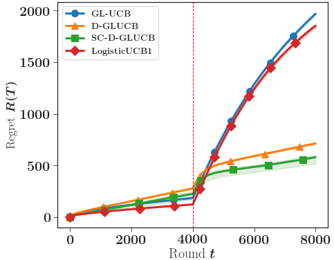
(a) $c_{\mu}^{-1}=400$

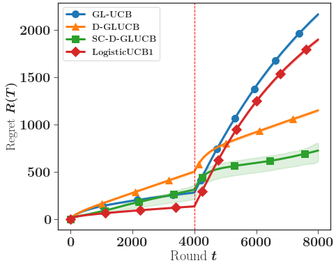
(b) $c_{\mu}^{-1}=1000$

Figure 1: Regret of the different algorithms in a 2D abruptly changing environment averaged on $200$ independent experiments and the $25\%$ associated quantiles.

Note that when $\hat{\theta}_{t}\in\Theta$ (i.e there is no need for a projection), our bound implies the one of Faury et al. (2020). The kind of relationship displayed in the above equation allows us to derive a tail inequality for the deviation from $\hat{\theta}_{t}$ to $\theta^{\star}$ without projecting $\hat{\theta}_{t}$, by solving an implicit equation. We believe that this new approach is of interest in other settings involving self-concordant GLBs. The self-concordance assumption (Assumption 4) is not particularly restrictive and goes beyond logistic functions. Under the classical Assumption 1 (i.e. bounded features) all GLMs are self-concordant (cf. Sec. 2 of Bach (2014)) with constants that depend on the link function.

6 EXPERIMENTS

In this section, we illustrate the empirical performance of $\tt SC\mathchar 45\relax D\mathchar 45\relax GLUCB$ in a simulated, abruptly changing environment with a logistic link function $\mu(x)=1/(1+\exp(-x))$. In this two-dimensional problem, there is a switch in the reward distribution at $t=4000$ (red dashed line on Figure 1).

$\tt SC\mathchar 45\relax D\mathchar 45\relax GLUCB$ (Algorithm 1) is compared with $\tt GLM\mathchar 45\relax UCB$ from Filippi et al. (2010), $\tt LogUCB1$ from Faury et al. (2020) and with $\tt D\mathchar 45\relax GLUCB$ from Russac et al. (2020). $\tt SC\mathchar 45\relax D\mathchar 45\relax GLUCB$ (resp. $\tt D\mathchar 45\relax GLUCB$) is related with $\tt LogUCB1$ (resp. $\tt GLM\mathchar 45\relax UCB$) in the sense that the exploration terms have the same scaling but the former incorporate the exponential weights making it possible to adapt to changes. The average regret of the different policies together with their central $50\%$ quantiles, averaged on 200 independent runs, are reported in Figure 1 for two different parameter values.

In Fig. 1(a), $\theta^{\star}$ starts on the circle of radius $S=6$ (corresponding to $c_{\mu}^{-1}=\exp(S)\approx 400$) with an angle of $2\pi/3$ and jumps at $t=4000$ to an angle of $4\pi/3$. The experiment reported on Fig. 1(b) is identical with a radius $S=7$ corresponding to a $c_{\mu}^{-1}\approx 1000$. As previously discussed, using such values of $S$ is required in situation where the actions return binary rewards with expected values in the range $10^{-3}$ – $10^{-2}$, which is typically the case in web advertising or recommendation applications.

For both experiments, at every time steps, $50$ randomly generated actions in the unit circle are proposed to the learner. For $\tt SC\mathchar 45\relax D\mathchar 45\relax GLUCB$ and $\tt D\mathchar 45\relax GLUCB$ the asymptotically optimal choice of the discount factors is used: $\gamma=1-(\Gamma_{T}/(d\times T))^{2/3}$ with $d=2$, $\Gamma_{T}=2$ and $T=8000$. To speed up the learning that is hard with those values of $c_{\mu}$, all the algorithms have their exploration bonus divided by 5.

As expected, the algorithms tuned for non stationary situations ($\tt SC\mathchar 45\relax D\mathchar 45\relax GLUCB$, $\tt D\mathchar 45\relax GLUCB$) perform worse than their stationary counterparts ($\tt LogUCB1$ and $\tt GLM\mathchar 45\relax UCB$) during the first stationary phase. More precisely, with the choice made for $\gamma$ the estimation of $\hat{\theta}_{t}$ for algorithms that use exponential weights is roughly based on the $1/(1-\gamma)\approx 400$ most recent observations. In contrast, $\tt LogUCB1$ and $\tt GLM\mathchar 45\relax UCB$ use all the observations from the start to compute the MLE, which eventually leads to a more precise estimation. Right after the change, the bias caused by the non-stationarity results in a significant increase in regret. Unweighted algorithms are affected much more deeply by this phenomenon that will eventually cause large losses in performance due to the persistence of obsolete information.

The theoretical analysis of Section 3.2 suggests that the advantage of $\tt SC\mathchar 45\relax D\mathchar 45\relax GLUCB$ is all the more significant in strongly non-linear (large $c_{\mu}^{-1}$) non-stationary environments. This is obvious in Figure 1, particularly when comparing Fig. 1(a) and Fig. 1(b), which differ by the range on which the logistic function is used for making reward predictions. Note that, on average, for these two simulated scenarios the fact that the MLE $\hat{\theta}_{t}$ does not belong to $\Theta$ happens for several hundred of rounds. All the algorithms except $\tt SC\mathchar 45\relax D\mathchar 45\relax GLUCB$ would require non convex projection steps at these instants, or equivalently, one should inflate $S$ (and thus $c_{\mu}^{-1}$) to ensure the compliance of these algorithms with the associated theory. In producing Figure 1, this projection step was simply bypassed, which provides an optimistic evaluation of the performance of the competitors of $\tt SC\mathchar 45\relax D\mathchar 45\relax GLUCB$. Interestingly, the observation that the dispersion of performance of $\tt SC\mathchar 45\relax D\mathchar 45\relax GLUCB$ is slightly higher than that of $\tt D\mathchar 45\relax GLUCB$ can be traced back to the use of Remark 1 in these simulations: $\tt SC\mathchar 45\relax D\mathchar 45\relax GLUCB$ adapts to the events $\{\hat{\theta}_{t}\notin\Theta\}$ (rather than pretending that these did not happen) and thus its performance is made somewhat dependent on the actual occurrence of these events.

 

Self-Concordant Analysis of Generalized Linear Bandits with Forgetting: Supplementary Material

 

The Appendix is structured as follows. In Section A, our new concentration result for self-normalized weighted martingales with time dependent regularization parameters is presented. In Section A.3, similar concentration results are established when a sliding window is used. Section B studies the regret with discount factors through our improved characterization of the MLE. Section C gives similar results with a sliding window. Section D gathers some technical results, in particular the main properties resulting from the self-concordance assumption. Finally in Section E, a worst case bound for a sliding window policy in the $K$-arm setting is presented.

Appendix A TAIL-INEQUALITY FOR SELF-NORMALIZED WEIGHTED MARTINGALES

While keeping in mind our objective of obtaining a deviation inequality with exponentially increasing weights, we give more generic results under two assumptions on the weights.

Assumption 6.

The time horizon $T$ is known in advance.

Assumption 7.

The weights are deterministic, strictly positive and non-decreasing, i.e,

$$\forall 1\leq t\leq T,0<w_{1}\leq w_{t}\leq w_{t+1}\leq w_{T}\;.$$

We recall the statement of the corresponding concentration result.

See 3

Theorem 3 is a non-trivial extension of Faury et al. (2020, Theorem 1) allowing for the use of time-dependent regularization parameters and weights. We now state several lemmas that are useful for establishing Theorem 3.

A.1 Useful Lemmas

As a first step we fix a time instant $t$. Let $M_{u}^{t}(\xi)$ for $\xi\in\mathbb{R}^{d}$ and $1\leq u\leq t$ be defined as

$$M_{u}^{t}(\xi)=\exp\left(\frac{1}{mw_{t-1}}\,\xi^{\top}S_{u}-\frac{1}{m^{2}w^{2}_{t-1}}\xi^{\top}\widetilde{\mathbf{H}}_{u}(0)\xi\right)\;,$$ (8)

with $S_{u}=\sum_{s=1}^{u-1}w_{s}\epsilon_{s+1}a_{s}$ and $\widetilde{\mathbf{H}}_{u}(0)=\sum_{s=1}^{u-1}w_{s}^{2}\sigma_{s}^{2}a_{s}a_{s}^{\top}$ where $\sigma_{s}^{2}=\mathbb{E}[\epsilon_{s+1}^{2}|\mathcal{F}_{s}]$.

We prefer the notation $M_{u}^{t}$ to $M_{u}$ to clearly indicate the dependency on the weight $w_{t-1}$. When $u=t$, we prefer the notation $M_{t}$ to $M_{t}^{t}$. For the entire appendix, we use the notation $\mathcal{B}_{2}(d)=\{a\in\mathbb{R}^{d},\lVert a\rVert_{2}\leq 1\}$.

Lemma 1.

For all $\xi\in\mathcal{B}_{2}(d)$ and $2\leq u\leq t$, under Assumption 6 and 7, we have

$$\mathbb{E}\left[M_{u}^{t}(\xi)|\mathcal{F}_{u-1}\right]\leq M_{u-1}^{t}(\xi)\;.\quad\text{a.s}$$

Proof.

$$\begin{split}\mathbb{E}\left[M_{u}^{t}(\xi)|\mathcal{F}_{u-1}\right]&=M_{u-1}^{t}(\xi)\exp\left(-\frac{1}{m^{2}w_{t-1}^{2}}\xi^{\top}w_{u-1}^{2}\sigma_{u-1}^{2}a_{u-1}a_{u-1}^{\top}\xi\right)\\ &\quad\times\mathbb{E}\left[\exp\left(\frac{1}{mw_{t-1}}\xi^{\top}w_{u-1}\epsilon_{u}a_{u-1}\right)|\mathcal{F}_{u-1}\right]\;.\end{split}$$

The equality holds because $a_{u-1}$ is $\mathcal{F}_{u-1}$ measurable and $\epsilon_{u-1}$ is $\mathcal{F}_{u-1}$ measurable. With $\tilde{\epsilon}_{u}=\epsilon_{u}/m$ and $v=\frac{w_{u-1}}{w_{t-1}}\xi^{\top}a_{u-1}$, the conditions of Lemma 3 (stated below) are met and we have,

$$\mathbb{E}\left[\exp\left(\frac{1}{mw_{t-1}}\xi^{\top}w_{u-1}\epsilon_{u}a_{u-1}\right)|\mathcal{F}_{u-1}\right]=\mathbb{E}\left[\exp(v\tilde{\epsilon}_{u})|\mathcal{F}_{u-1}\right]\leq 1+\frac{v^{2}}{m^{2}}\sigma_{u-1}^{2}\;.$$

$|v|\leq 1$ holds because of Assumption 7 and both $\xi$ and $a_{u-1}\in\mathcal{B}_{2}(d)$. Therefore,

$$\begin{split}\mathbb{E}\left[M_{u}^{t}(\xi)|\mathcal{F}_{u-1}\right]&\leq M_{u-1}^{t}(\xi)\exp\left(-\frac{1}{m^{2}w_{t-1}^{2}}\xi^{\top}w_{u-1}^{2}\sigma_{u-1}^{2}a_{u-1}a_{u-1}^{\top}\xi\right)\\ &\quad\times\left(1+\frac{w_{u-1}^{2}}{m^{2}w_{t-1}^{2}}\sigma^{2}_{u-1}\xi^{\top}a_{u-1}a_{u-1}^{\top}\xi\right)\\ &\leq M_{u-1}^{t}(\xi)\quad\text{(a.s)}\;,\end{split}$$

where the last inequality uses $1+x\leq\exp(x)$. ∎

Hence, for all $1\leq u\leq t$ and $\xi\in\mathcal{B}_{2}(d)$, $\mathbb{E}\left[M_{t}(\xi)\right]\leq\mathbb{E}\left[M_{u}^{t}(\xi)\right]\leq\mathbb{E}\left[M_{1}^{t}(\xi)\right]=1$.

For $1\leq u\leq t$ we define,

$$\bar{M}_{u}^{t}=\int_{\xi}M_{u}^{t}(\xi)dh_{u}(\xi)\;.$$ (9)

Here, $h_{u}$ is the density of an isotropic normal distribution of precision $\frac{2\lambda_{u-1}}{m^{2}w_{t-1}^{2}}$ truncated on $\mathcal{B}_{2}(d)$. We will denote $N(h_{u})$ its normalization constant.

Lemma 2.

Let $t$ be a fixed time instant, for all $1\leq u\leq t$, under assumptions 6 and 7, with $\{h_{u}\}_{u=1}^{t}$ the density of an isotropic normal distribution of precision $\frac{2\lambda_{u-1}}{m^{2}w_{t-1}^{2}}$ truncated on $\mathcal{B}_{2}(d)$ we have,

$$\mathbb{E}\left[\bar{M}_{u}^{t}\right]\leq 1\;.$$

Proof.

$$\mathbb{E}\left[\bar{M}_{u}^{t}\right] =\int_{\Omega}\bar{M}_{u}^{t}d\mathbb{P}(w)=\int_{\Omega}\left(\int_{\mathbb{R}^{d}}M_{u}^{t}(\xi)dh_{u}(\xi)\right)d\mathbb{P}(w)$$

$$\leq\int_{\mathbb{R}^{d}}\left(\int_{\Omega}M_{u}^{t}(\xi)d\mathbb{P}(w)\right)dh_{u}(\xi)\quad\text{(Fubini)}$$

$$\leq\int_{\mathbb{R}^{d}}\left(\int_{\Omega}1d\mathbb{P}(w)\right)dh_{u}(\xi)\quad\text{(Lemma \ref{lemma_instantaneous} + $h_{u}$ defined on $\mathcal{B}_{2}(d)$)}$$

$$\leq\int_{\mathbb{R}^{d}}dh_{u}(\xi)=1\;.\quad\text{($h_{u}$ is a probability density function)}$$

∎

Remark 2.

Allowing time-dependent regularization parameters is essential in our analysis to avoid the vanishing effect of the regularization with exponentially increasing weights for example. This is a fundamental difference with the deviation result provided in Faury et al. (2020). Furthermore, allowing the regularization parameters to be time-dependent comes at a cost here, we loose the property $\mathbb{E}\left[\bar{M}_{u}^{t}|\mathcal{F}_{u-1}\right]\leq\bar{M}_{u-1}^{t}$ that would hold with a fixed regularization parameter (as in Faury et al. (2020)). In the linear bandit setting, this issue was discussed in Lemma 2 in Russac et al. (2019).

In particular, applying Lemma 2 for $u=t$ gives,

$$\mathbb{E}\left[\bar{M}_{t}\right]=\mathbb{E}\left[\bar{M}_{t}^{t}\right]\leq 1\;.$$ (10)

Lemma 3 (Lemma 7 of Faury et al. (2020)).

Let $\varepsilon$ be a centered random variable of variance $\sigma^{2}$ and such that $|\varepsilon|\leq 1$ almost surely. Then for all $v\in[-1,1]$,

$$\mathbb{E}\left[\exp(v\varepsilon)\right]\leq 1+v^{2}\sigma^{2}\;.$$

Remark 3.

We stress out that $v\in[-1,1]$ is required for Lemma 3 to hold. It has strong consequences in our setting with the weights as the normalization $1/w_{t-1}$ and $1/w_{t-1}^{2}$ in the definition of $M_{u}^{t}\;$ are needed to ensure that $v=(w_{u-1}/w_{t-1})\xi^{\top}a_{u}$ that appears in the proof of Lemma 1 will be smaller than 1. As a consequence, the stopping trick presented in Abbasi-Yadkori et al. (2011) can not be applied to $\bar{M}_{u}^{t}$ because of its dependency on $t$. For this reason, the deviation result presented in Theorem 3 is only valid for a fixed time instant $t$. To obtain a deviation result on the entire trajectory an union bound is required.

A.2 Proof of Theorem 3

The proof of this theorem follows the line of proof of Faury et al. (2020). The main differences are the time-dependent regularization parameters and the presence of weights. We recall that in Equation (9) $h_{t}$ is the density of an isotropic normal distribution of precision $\frac{2\lambda_{t-1}}{m^{2}w_{t-1}^{2}}$ truncated on $\mathcal{B}_{2}(d)$ and denote $N(h_{t})$ its normalization constant.

The following holds,

$$\bar{M}_{t}=\frac{1}{N(h_{t})}\int_{\mathbb{R}^{d}}\mathds{1}\left[\xi\in\mathcal{B}_{2}(d)\right]\exp\left(\frac{1}{mw_{t-1}}\xi^{\top}S_{t}-\frac{1}{m^{2}w_{t-1}^{2}}\xi^{\top}\widetilde{\mathbf{H}}_{t}\xi\right)d\xi\;.$$ (11)

Let $f_{t}:\mathbb{R}^{d}\mapsto\mathbb{R}$ be defined as $f_{t}(\xi)=\frac{1}{mw_{t-1}}\xi^{\top}S_{t}-\frac{1}{m^{2}w_{t-1}^{2}}\xi^{\top}\widetilde{\mathbf{H}}_{t}\xi$. As a quadratic function, $f_{t}$ can be rewritten for $\xi^{\star}=\operatorname*{arg\,max}_{\lVert\xi\rVert_{2}\leq 1/2}f_{t}(\xi)$,

$$f_{t}(\xi)=f_{t}(\xi^{\star})+\nabla f_{t}(\xi^{\star})^{\top}(\xi-\xi^{\star})+\frac{1}{2}(\xi-\xi^{\star})^{\top}\nabla^{2}f_{t}(\xi^{\star})(\xi-\xi^{\star})\;.$$

Using $\forall\xi\in\mathcal{B}_{2}(d),\,\,\nabla^{2}f_{t}(\xi)=-\frac{2}{m^{2}w_{t-1}^{2}}\widetilde{\mathbf{H}}_{t}$,

$$\bar{M}_{t} =\frac{e^{f_{t}(\xi^{\star})}}{N(h_{t})}\int_{\mathbb{R}^{d}}\mathds{1}\left[\lVert\xi\rVert_{2}\leq 1\right]\exp\left(\nabla f_{t}(\xi^{\star})^{\top}(\xi-\xi^{\star})-\frac{1}{m^{2}w_{t-1}^{2}}\lVert\xi-\xi^{\star}\rVert_{\widetilde{\mathbf{H}}_{t}}^{2}\right)d\xi$$

$$=\frac{e^{f_{t}(\xi^{\star})}}{N(h_{t})}\int_{\mathbb{R}^{d}}\mathds{1}\left[\lVert\xi+\xi^{\star}\rVert_{2}\leq 1\right]\exp\left(\nabla f_{t}(\xi^{\star})^{\top}\xi-\frac{1}{m^{2}w_{t-1}^{2}}\lVert\xi\rVert_{\widetilde{\mathbf{H}}_{t}}^{2}\right)d\xi$$

$$\geq\frac{e^{f_{t}(\xi^{\star})}}{N(h_{t})}\int_{\mathbb{R}^{d}}\mathds{1}\left[\lVert\xi\rVert_{2}\leq 1/2\right]\exp\left(\nabla f_{t}(\xi^{\star})^{\top}\xi-\frac{1}{m^{2}w_{t-1}^{2}}\lVert\xi\rVert_{\widetilde{\mathbf{H}}_{t}}^{2}\right)d\xi$$

$$\geq\frac{e^{f_{t}(\xi^{\star})}N(g_{t})}{N(h_{t})}\mathbb{E}_{\xi\sim g_{t}}\left[\exp\left(\nabla f_{t}(\xi^{\star})^{\top}\xi\right)\right]\;.$$

The second equality is obtained after a change of variable $\xi\mapsto\xi-\xi^{\star}$. In the last inequality, $g_{t}$ is the density of a $d$-dimensional normal distribution with precision matrix $\frac{2}{m^{2}w_{t-1}^{2}}\widetilde{\mathbf{H}}_{t}$ truncated on $\{a\in\mathbb{R}^{d},\lVert a\rVert_{2}\leq 1/2\}$.

$$\bar{M}_{t} \geq\frac{e^{f_{t}(\xi^{\star})}N(g_{t})}{N(h_{t})}\exp\left(\mathbb{E}_{\xi\sim g_{t}}\left[\nabla f_{t}(\xi^{\star})^{\top}\xi\right]\right)\;.\quad\textnormal{(Jensen's inequality)}$$

$g_{t}$ is symmetric which implies $\mathbb{E}_{\xi\sim g_{t}}\left[\xi\right]=0$. Hence,

$$\bar{M}_{t}\geq\frac{e^{f_{t}(\xi^{\star})}N(g_{t})}{N(h_{t})}\;.$$ (12)

Therefore,

$$\delta \geq\mathbb{P}\left(\bar{M}_{t}\geq\frac{1}{\delta}\right)\quad\text{(Equation \eqref{eq_bar_t} + Markov's Inequality)}$$

$$\geq\mathbb{P}\left(f_{t}(\xi^{\star})\geq\log\left(\frac{1}{\delta}\right)+\log\left(\frac{N(h_{t})}{N(g_{t})}\right)\right)\quad\textnormal{(Equation $\eqref{eq:bar_M_t_lower}$)}$$

$$=\mathbb{P}\left(\max_{\lVert\xi\rVert_{2}\leq 1/2}f_{t}(\xi)\geq\log\left(\frac{1}{\delta}\right)+\log\left(\frac{N(h_{t})}{N(g_{t})}\right)\right)$$

$$\geq\mathbb{P}\left(f_{t}(\xi_{0})\geq\log\left(\frac{1}{\delta}\right)+\log\left(\frac{N(h_{t})}{N(g_{t})}\right)\right)\;.$$

In the last inequality $\xi_{0}$ is defined as $\xi_{0}=\frac{\sqrt{\lambda_{t}}}{2}\frac{\widetilde{\mathbf{H}}_{t}^{-1}S_{t}}{\lVert S_{t}\rVert_{\widetilde{\mathbf{H}}_{t}^{-1}}}$, such that $\lVert\xi_{0}\rVert_{2}\leq 1/2$ holds. This can be seen by using $\widetilde{\mathbf{H}}_{t}\geq\lambda_{t-1}\mathbf{I}_{d}$. We also have,

$$f_{t}(\xi_{0})=\frac{1}{mw_{t-1}}\xi_{0}^{\top}S_{t}-\frac{1}{m^{2}w_{t-1}^{2}}\xi_{0}^{\top}\widetilde{\mathbf{H}}_{t}\xi_{0}=\frac{\sqrt{\lambda_{t-1}}}{2mw_{t-1}}\lVert S_{t}\rVert_{\widetilde{\mathbf{H}}_{t}^{-1}}-\frac{\lambda_{t-1}}{4m^{2}w_{t-1}^{2}}\;.$$

Therefore,

$$\mathbb{P}\left(\lVert S_{t}\rVert_{\widetilde{\mathbf{H}}_{t}^{-1}}\geq\frac{\sqrt{\lambda_{t-1}}}{2mw_{t-1}}+\frac{2mw_{t-1}}{\sqrt{\lambda_{t-1}}}\log(1/\delta)+\frac{2mw_{t-1}}{\sqrt{\lambda_{t-1}}}\log\left(\frac{N(h_{t})}{N(g_{t})}\right)\right)\leq\delta\;.$$ (13)

We conclude using Proposition 2.

Proposition 2.

Let $h_{t}$ be the density of a $d$-dimensional isotropic normal distribution of precision $\frac{2\lambda_{t-1}}{m^{2}w_{t-1}^{2}}$ truncated on $\mathcal{B}_{2}(d)$. Let $g_{t}$ be the density of a $d$-dimensional normal distribution with precision matrix $\frac{2}{m^{2}w_{t-1}^{2}}\widetilde{\mathbf{H}}_{t}$ truncated on $\{a\in\mathbb{R}^{d},\lVert a\rVert_{2}\leq 1/2\}$. The following inequality holds,

$$\log\left(\frac{N(h_{t})}{N(g_{t})}\right)\leq\log\left(\frac{\det(\widetilde{\mathbf{H}}_{t})}{\lambda_{t-1}^{d/2}}\right)+d\log(2)\;.$$ (14)

Proof.

$$N(h_{t}) =\int_{\mathbb{R}^{d}}\mathds{1}\left[\lVert\xi\rVert_{2}\leq 1\right]\exp\left(-\frac{1}{2}\frac{2\lambda_{t-1}}{m^{2}w_{t-1}^{2}}\lVert\xi\rVert_{2}^{2}\right)d\xi$$

$$=\left(\frac{m^{2}w_{t-1}^{2}}{2\lambda_{t-1}}\right)^{d/2}\int_{\mathbb{R}^{d}}\mathds{1}\left[\lVert\xi\rVert_{2}\leq\frac{\sqrt{2\lambda_{t-1}}}{mw_{t-1}}\right]\exp\left(-\frac{1}{2}\lVert\xi\rVert_{2}^{2}\right)d\xi\;.$$

$$N(g_{t}) =\int_{\mathbb{R}^{d}}\mathds{1}\left[\lVert\xi\rVert_{2}\leq 1/2\right]\exp\left(-\frac{1}{2}\frac{2}{m^{2}w_{t-1}^{2}}\xi^{\top}\widetilde{\mathbf{H}}_{t}\xi\right)d\xi$$

$$=\frac{1}{\left|\det\left(\frac{\sqrt{2}}{mw_{t-1}}\widetilde{\mathbf{H}}_{t}^{1/2}\right)\right|}\int_{\mathbb{R}^{d}}\mathds{1}\left[\lVert\xi\rVert_{2}\leq\frac{1}{2}\frac{\sqrt{2\lambda_{t-1}}}{mw_{t-1}}\right]\exp\left(-\frac{1}{2}\lVert\xi\rVert_{2}^{2}\right)d\xi$$

$$\geq\left(\frac{m^{2}w_{t-1}^{2}}{2}\right)^{d/2}\det(\widetilde{\mathbf{H}}_{t})^{-1/2}\int_{\mathbb{R}^{d}}\mathds{1}\left[\lVert\xi\rVert_{2}\leq\frac{1}{2}\frac{\sqrt{2\lambda_{t-1}}}{mw_{t-1}}\right]\exp\left(-\frac{1}{2}\lVert\xi\rVert_{2}^{2}\right)d\xi\;.$$

Therefore,

$$\frac{N(h_{t})}{N(g_{t})}\leq\frac{\det(\widetilde{\mathbf{H}}_{t})}{\lambda_{t-1}^{d/2}}\underbrace{\frac{\int_{\mathbb{R}^{d}}\mathds{1}\left[\lVert\xi\rVert_{2}\leq\frac{\sqrt{2\lambda_{t-1}}}{mw_{t-1}}\right]\exp\left(-\frac{1}{2}\lVert\xi\rVert_{2}^{2}\right)d\xi}{\int_{\mathbb{R}^{d}}\mathds{1}\left[\lVert\xi\rVert_{2}\leq\frac{1}{2}\frac{\sqrt{2\lambda_{t-1}}}{mw_{t-1}}\right]\exp\left(-\frac{1}{2}\lVert\xi\rVert_{2}^{2}\right)d\xi}}_{R}\;.$$ (15)

The last step consists in upper bounding the ratio of the integrals $R$. Following, (Faury et al., 2020, Lemma 6), one gets $R=2^{d}$.

We conclude by using this equality in Equation (15) and applying the logarithm on both sides. ∎

A.3 A Unifying Concentration Result for Discount Factors and Sliding-Window

In this section, we explain how Theorem 3 can be used with self-concordant GLBs to obtain a concentration inequality that encapsulates the analysis for both discount-factors and the sliding-window.

Up to now, we have stated the results in the most generic way. Actually, in our analysis we will use a weaker version of the concentration inequality established in Theorem 3.

Theorem 4.

Let $t$ be a fixed time instant. Let $\{\mathcal{F}_{u}\}_{u=1}^{t}$ be a filtration. Let $\{a_{u}\}_{u=1}^{t}$ be a stochastic process on $\mathbb{R}^{d}$ such that $a_{u}$ is $\mathcal{F}_{u}$ measurable and $\lVert a_{u}\rVert_{2}\leq 1$. Let $\{\epsilon_{u}\}_{u=2}^{t}$ be a martingale difference sequence such that $\epsilon_{u+1}$ is $\mathcal{F}_{u+1}$ measurable. Assume that the weights are non-decreasing, positive and the time horizon is known. Furthermore, assume that conditionally on $\mathcal{F}_{u}$ we have $|\epsilon_{u+1}|\leq m$ a.s. Let $\{\lambda_{u}\}_{u=1}^{t}$ be a deterministic sequence of regularization terms and denote $\sigma_{t}^{2}=\mathbb{E}\left[\epsilon_{t+1}^{2}|\mathcal{F}_{t}\right]$.

Let $\widetilde{\mathbf{H}}_{t-t_{0}:t}=\sum_{s=t-t_{0}}^{t-1}w_{s}^{2}\sigma_{s}^{2}a_{s}a_{s}^{\top}+\lambda_{t-1}\mathbf{I}_{d}$ and $S_{t-t_{0}:t}=\sum_{s=t-t_{0}}^{t-1}w_{s}\epsilon_{s+1}a_{s}$.

Then for any $\delta\in(0,1]$,

$$\mathbb{P}\left(\left\lVert S_{t-t_{0}:t}\right\rVert_{\widetilde{\mathbf{H}}_{t-t_{0}:t}^{-1}}\geq\frac{\sqrt{\lambda_{t-1}}}{2mw_{t-1}}+\frac{2mw_{t-1}}{\sqrt{\lambda_{t-1}}}\log\left(\frac{\det(\widetilde{\mathbf{H}}_{t-t_{0}:t})^{1/2}}{\delta\lambda_{t-1}^{d/2}}\right)+\frac{2mw_{t-1}}{\sqrt{\lambda_{t-1}}}d\log(2)\right)\leq\delta\;.$$

Proof.

The arguments used to establish Theorem 4 are the same than for Theorem 3. We only give the main term that differs from the proof of Theorem 3.

With $t$ a fixed time instant, for any $u$ such that $t-t_{0}\leq u\leq t$, $M_{u}^{t}$ is defined as

$$M_{u}^{t}(\xi)=\exp\left(\frac{1}{mw_{t-1}}\,\xi^{\top}S_{t-t_{0}:u}-\frac{1}{m^{2}w_{t-1}^{2}}\xi^{\top}\sum_{s=t-t_{0}}^{u-1}w_{s}^{2}a_{s}a_{s}^{\top}\xi\right)\;,$$

with $S_{t-t_{0}:u}=\sum_{s=t-t_{0}}^{u-1}w_{s}\epsilon_{s+1}a_{s}$. Following the steps of the proof of Theorem 3 with these slight differences gives the result. ∎

Discount Factors

Let $t_{0}=D$ be the equivalent of the sliding window length with exponential weights, $w_{t}=\gamma^{-t}$ and $\lambda_{t}=\lambda\gamma^{-2t}$ for $0<\gamma<1$. Even when $\gamma$ depends on $T$, the weights satisfy the assumptions 6 and 7. We can obtain:

Corollary 1 (Concentration result with discount factors).

Under the same assumption than Theorem 4, when defining $\widetilde{\mathbf{H}}_{t-D:t}=\sum_{s=t-D}^{t-1}\gamma^{2(t-1-s)}\dot{\mu}(a_{s}^{\top}\theta^{\star}_{s})a_{s}a_{s}^{\top}+\lambda\mathbf{I}_{d}$ and $S_{t-D:t}=\sum_{s=t-D}^{t-1}\gamma^{-s}\epsilon_{s+1}a_{s}$. For any $\delta\in(0,1]$,

$$\mathbb{P}\left(\left\lVert\gamma^{t-1}S_{t-D:t}\right\rVert_{\widetilde{\mathbf{H}}_{t-D:t}^{-1}}\geq\frac{\sqrt{\lambda}}{2m}+\frac{2m}{\sqrt{\lambda}}\log\left(\frac{\det(\widetilde{\mathbf{H}}_{t-D:t})^{1/2}}{\delta\lambda^{d/2}}\right)+\frac{2m}{\sqrt{\lambda}}d\log(2)\right)\leq\delta\;.$$

Sliding Window

With $t_{0}=\tau$ the length of the sliding window, with the weights satisfying $w_{t}=1$ for $t-\tau\leq s\leq t-1$ and $\lambda_{t}=\lambda$, we have:

Corollary 2 (Concentration result with a sliding window).

Under the same assumption than Theorem 4, when defining $\mathbf{H}_{t}=\sum_{s=\max(1,t-\tau)}^{t-1}\dot{\mu}(a_{s}^{\top}\theta^{\star}_{s})a_{s}a_{s}^{\top}+\lambda\mathbf{I}_{d}$ and $S_{t}=\sum_{s=\max(1,t-\tau)}^{t-1}\epsilon_{s+1}a_{s}$. For any $\delta\in(0,1]$,

$$\mathbb{P}\left(\left\lVert S_{t}\right\rVert_{\mathbf{H}_{t}^{-1}}\geq\frac{\sqrt{\lambda}}{2m}+\frac{2m}{\sqrt{\lambda}}\log\left(\frac{\det(\mathbf{H}_{t})^{1/2}}{\delta\lambda^{d/2}}\right)+\frac{2m}{\sqrt{\lambda}}d\log(2)\right)\leq\delta\;.$$

Appendix B REGRET ANALYSIS WITH DISCOUNT FACTORS

In this section we detail the regret analysis of $\tt SC\mathchar 45\relax D\mathchar 45\relax GLUCB$. First we recall the main notation.

B.1 Notation

For any $\theta\in\mathbb{R}^{d}$,

$$\widetilde{\mathbf{H}}_{t}(\theta)=\sum_{s=1}^{t-1}\gamma^{2(t-1-s)}\dot{\mu}(a_{s}^{\top}\theta)a_{s}a_{s}^{\top}+\lambda\mathbf{I}_{d}\;.$$ (16)

$$\mathbf{H}_{t}(\theta)=\sum_{s=1}^{t-1}\gamma^{t-1-s}\dot{\mu}(a_{s}^{\top}\theta)a_{s}a_{s}^{\top}+\lambda\mathbf{I}_{d}\;.$$ (17)

$$\mathbf{\widetilde{V}}_{t}=\sum_{s=1}^{t-1}\gamma^{2(t-1-s)}a_{s}a_{s}^{\top}+\frac{\lambda}{c_{\mu}}\mathbf{I}_{d}\;.$$ (18)

$$\mathbf{V}_{t}=\sum_{s=1}^{t-1}\gamma^{t-1-s}a_{s}a_{s}^{\top}+\frac{\lambda}{c_{\mu}}\mathbf{I}_{d}\;.$$ (19)

$$g_{1:t}(\theta)=\sum_{s=1}^{t-1}\gamma^{t-1-s}\mu(a_{s}^{\top}\theta)a_{s}+\lambda\theta\;.$$ (20)

$$S_{t}=\sum_{s=1}^{t-1}\gamma^{-s}\epsilon_{s+1}a_{s}\;.$$ (21)

For any $\theta_{1},\theta_{2}\in\mathbb{R}^{d}$,

$$\alpha(a,\theta_{1},\theta_{2})=\int_{0}^{1}\dot{\mu}(va^{\top}\theta_{2}+(1-v)a^{\top}\theta_{1})dv\;.$$

$$\mathbf{G}_{t}(\theta_{1},\theta_{2})=\sum_{s=1}^{t-1}\gamma^{t-1-s}\alpha(a_{s},\theta_{1},\theta_{2})a_{s}a_{s}^{\top}+\lambda\mathbf{I}_{d}\;.$$

$$\widetilde{\mathbf{G}}_{t}(\theta_{1},\theta_{2})=\sum_{s=1}^{t-1}\gamma^{2(t-1-s)}\alpha(a_{s},\theta_{1},\theta_{2})a_{s}a_{s}^{\top}+\lambda\mathbf{I}_{d}\;.$$ (22)

Let $\widetilde{\mathbf{H}}_{t}$ be defined as

$$\widetilde{\mathbf{H}}_{t}=\sum_{s=1}^{t-1}\gamma^{2(t-1-s)}\dot{\mu}(a_{s}^{\top}\theta^{\star}_{s})a_{s}a_{s}^{\top}+\lambda\mathbf{I}_{d}\;.$$ (23)

Let us define $\mathcal{T}(\gamma)$ as

$$\mathcal{T}(\gamma)=\{1\leq t\leq T,\text{such that}\,\forall s,\,t-D\leq s\leq t-1,\theta^{\star}_{s}=\theta^{\star}_{t}\}\;.$$ (24)

Remark.

$t\in\mathcal{T}(\gamma)$ when $t$ is a least $D$ steps away from the closest previous breakpoint. On the contrary to the analysis with the sliding window (see Appendix C) the bias does not completely cancel out when we are far enough from a breakpoint.

$D$ is an analysis parameter and will be specified later in the different theorems. For the entire section we will use the notation $t-D:t$ when the sum concerns time instants $s$ such that $t-D\leq s\leq t-1$. In the weighted setting, we construct an estimator based on a weighted penalized log-likelihood. $\hat{\theta}_{t}$ is defined as the unique maximizer of

$$\sum_{s=1}^{t-1}\gamma^{t-1-s}\log\mathbb{P}_{\theta}(r_{s+1}|a_{s})-\frac{\lambda}{2}\lVert\theta\rVert_{2}^{2}\;.$$

By using the definition of the GLM and thanks to the concavity of this equation in $\theta$, $\hat{\theta}_{t}$ is the unique solution of

$$\sum_{s=1}^{t-1}\gamma^{t-1-s}(r_{s+1}-\mu(a_{s}^{\top}\theta))a_{s}-\lambda\theta=0\;.$$

This can be summarized with

$$g_{1:t}(\hat{\theta}_{t}) =\sum_{s=1}^{t-1}\gamma^{t-1-s}r_{s+1}a_{s}=\gamma^{t-1}S_{t}+\sum_{s=1}^{t-1}\gamma^{t-1-s}\mu(a_{s}^{\top}\theta^{\star}_{s})a_{s}\;.$$ (25)

B.2 Analysis of the Regret of $\tt SC\mathchar 45\relax D\mathchar 45\relax GLUCB$

In this section, we present the main ideas to obtain an analysis of the regret of the $\tt SC\mathchar 45\relax D\mathchar 45\relax GLUCB$ algorithm when the projection step is avoided.

We define

$$\rho_{T}^{\delta}=\left(\frac{\sqrt{\lambda}}{2m}+\frac{2m}{\sqrt{\lambda}}\log\left(\frac{T}{\delta}\right)+\frac{dm}{\sqrt{\lambda}}\log\left(1+\frac{k_{\mu}(1-\gamma^{2D})}{d\lambda(1-\gamma^{2})}\right)+\frac{2m}{\sqrt{\lambda}}d\log(2)\right)\;,$$ (26)

and also,

$$\bar{S}=S+\frac{\gamma^{D}(2Sk_{\mu}+m)}{\lambda(1-\gamma)}\;.$$ (27)

The expression of $\rho_{T}^{\delta}$ and $\bar{S}$ given here coincide with the expression in the main paper when $D=\log(T)/\log(1/\gamma)$. $\rho_{T}^{\delta}$ is defined such that thanks to Corollary 1 with high probability for all $t$ in $\mathcal{T}(\gamma)$, $\lVert\gamma^{t-1}S_{t-D:t}\rVert_{\widetilde{\mathbf{H}}_{t-D:t}^{-1}}\leq\rho^{\delta}_{T}$ holds.

The next result uses the self-concordance to relate the first derivative of the link function evaluated at different points. This relation is independent of $c_{\mu}$ and only depends on the distance between the parameters.

Proposition 3.

When $\hat{\theta}_{t}$ is the maximum likelihood as defined in Equation (1) and $t\in\mathcal{T}(\gamma)$, we have

$$\alpha(a,\theta^{\star}_{t},\hat{\theta}_{t})\geq\left(1+\bar{S}+\frac{1}{\sqrt{\lambda}}\lVert\gamma^{t-1}S_{t-D:t}\rVert_{\widetilde{\mathbf{G}}_{t-D:t}^{-1}(\theta^{\star}_{t},\hat{\theta}_{t})}\right)^{-1}\dot{\mu}(a^{\top}\theta^{\star}_{t})\;,$$

where $\bar{S}$ is defined in Equation (27).

Proof.

In the proof, we will replace the notation $\widetilde{\mathbf{G}}_{t-D:t}(\theta^{\star}_{t},\hat{\theta}_{t})$ with $\widetilde{\mathbf{G}}_{t-D:t}$ and $\widetilde{\mathbf{G}}_{t}(\theta^{\star}_{t},\hat{\theta}_{t})$ with $\widetilde{\mathbf{G}}_{t}$ but also $\mathbf{G}_{t}(\theta^{\star}_{t},\hat{\theta}_{t})$ with $\mathbf{G}_{t}$. Using Lemma 4 we have,

$$\alpha(a,\theta^{\star}_{t},\hat{\theta}_{t})\geq\left(1+\left|a^{\top}(\hat{\theta}_{t}-\theta^{\star}_{t})\right|\right)^{-1}\dot{\mu}(a^{\top}\theta^{\star}_{t})\;.$$

Combining this with the mean value theorem gives

$$\alpha(a,\theta^{\star}_{t},\hat{\theta}_{t})\geq\left(1+\left|a^{\top}\mathbf{G}_{t}^{-1}\left(g_{1:t}(\hat{\theta}_{t})-g_{1:t}(\theta^{\star}_{t})\right)\right|\right)^{-1}\dot{\mu}(a^{\top}\theta^{\star}_{t})\;.$$

Next, it is possible to upper bound $|a^{\top}\mathbf{G}_{t}^{-1}\left(g_{1:t}(\hat{\theta}_{t})-g_{1:t}(\theta^{\star}_{t})\right)|$ using the triangle inequality and Equation (25).

$$\begin{split}\left|a^{\top}\mathbf{G}_{t}^{-1}\left(g_{1:t}(\hat{\theta}_{t})-g_{1:t}(\theta^{\star}_{t})\right)\right|&\leq\underbrace{\left|a^{\top}\mathbf{G}_{t}^{-1}\sum_{s=1}^{t-1}\gamma^{t-1-s}(\mu(a_{s}^{\top}\theta^{\star}_{s})-\mu(a_{s}^{\top}\theta^{\star}_{t}))a_{s}\right|}_{b_{1,t}(a)}\\ &\quad+\underbrace{\left|a^{\top}\mathbf{G}_{t}^{-1}\left(-\lambda\theta^{\star}_{t}+\sum_{s=1}^{t-D-1}\gamma^{t-1-s}\epsilon_{s+1}a_{s}\right)\right|}_{b_{2,t}(a)}\\ &\quad+\underbrace{\left|a^{\top}\mathbf{G}_{t}^{-1}\gamma^{t-1}S_{t-D:t}\right|}_{b_{3,t}(a)}\end{split}$$

The first term is controlled as follows,

$$b_{1,t}(a) =\left|a^{\top}\mathbf{G}_{t}^{-1}\sum_{s=1}^{t-1}\gamma^{t-1-s}(\mu(a_{s}^{\top}\theta^{\star}_{s})-\mu(a_{s}^{\top}\theta^{\star}_{t}))a_{s}\right|$$

$$\leq\lVert a\rVert_{\mathbf{G}_{t}^{-1}}\lVert\sum_{s=1}^{t-1}\gamma^{t-1-s}(\mu(a_{s}^{\top}\theta^{\star}_{s})-\mu(a_{s}^{\top}\theta^{\star}_{t}))a_{s}\rVert_{\mathbf{G}_{t}^{-1}}\quad\text{(Cauchy-Schwarz ineq.)}$$

$$\leq\frac{1}{\sqrt{\lambda}}\lVert\sum_{s=1}^{t-D-1}\gamma^{t-1-s}(\mu(a_{s}^{\top}\theta^{\star}_{s})-\mu(a_{s}^{\top}\theta^{\star}_{t}))a_{s}\rVert_{\mathbf{G}_{t}^{-1}}\quad(\mathbf{G}_{t}\geq\lambda\mathbf{I}_{d}\;\text{and}\;t\in\mathcal{T}(\gamma))$$

$$\leq\frac{1}{\lambda}\sum_{s=1}^{t-D-1}\gamma^{t-1-s}|\alpha(a_{s},\theta^{\star}_{s},\theta^{\star}_{t})|\times|a_{s}^{\top}(\theta^{\star}_{t}-\theta^{\star}_{s})|\times\lVert a_{s}\rVert_{2}\quad(\text{Triangle ineq.}+\mathbf{G}_{t}\geq\lambda\mathbf{I}_{d})$$

$$\leq\frac{2Sk_{\mu}}{\lambda}\sum_{s=1}^{t-D-1}\gamma^{t-1-s}\quad(\theta^{\star}_{s}\;\text{and}\;\theta^{\star}_{t}\in\Theta)$$

$$\leq\frac{2Sk_{\mu}}{\lambda}\frac{\gamma^{D}}{1-\gamma}\;.$$

Using similar arguments, one can upper bound $b_{2,t}(a)$.

$$b_{2,t}(a) =\left|a^{\top}\mathbf{G}_{t}^{-1}\left(-\lambda\theta^{\star}_{t}+\sum_{s=1}^{t-D-1}\gamma^{t-1-s}\epsilon_{s+1}a_{s}\right)\right|$$

$$\leq S+\lVert\sum_{s=1}^{t-D-1}\gamma^{t-1-s}\epsilon_{s+1}a_{s}\rVert_{\mathbf{G}_{t}^{-2}}$$

$$\leq S+\frac{m}{\lambda}\frac{\gamma^{D}}{1-\gamma}\;.\quad(|\epsilon_{s+1}|\leq m)$$

Before upper bounding, $b_{3,t}(a)$, we need the following relation.

When $0<\gamma<1$, $\gamma^{2(t-1-s)}\leq\gamma^{t-1-s}$ for $s$ smaller than $t-1$ which implies

$$\forall\theta_{1},\theta_{2}\in\mathbb{R}^{d},\;\widetilde{\mathbf{G}}_{t}(\theta_{1},\theta_{2})\leq\mathbf{G}_{t}(\theta_{1},\theta_{2})\;.$$ (28)

We have,

$$b_{3,t}(a) =|a^{\top}\mathbf{G}_{t}^{-1}\widetilde{\mathbf{G}}_{t}^{1/2}\widetilde{\mathbf{G}}_{t}^{-1/2}\gamma^{t-1}S_{t-D:t}|$$

$$\leq\lVert a\rVert_{\mathbf{G}_{t}^{-1}\widetilde{\mathbf{G}}_{t}\mathbf{G}_{t}^{-1}}\lVert\gamma^{t-1}S_{t-D:t}\rVert_{\widetilde{\mathbf{G}}^{-1}_{t}}\quad\text{(Cauchy-Schwarz ineq.)}$$

$$\leq\lVert a\rVert_{\mathbf{G}_{t}^{-1}}\lVert\gamma^{t-1}S_{t-D:t}\rVert_{\widetilde{\mathbf{G}}^{-1}_{t}}\quad\textnormal{(Equation \eqref{eq:link_G_t_G_t_tilde})}$$

$$\leq\frac{1}{\sqrt{\lambda}}\lVert\gamma^{t-1}S_{t-D:t}\rVert_{\widetilde{\mathbf{G}}_{t-D:t}^{-1}}\;.\quad(\mathbf{G}_{t}\geq\lambda\mathbf{I}_{d})$$

By combining all the results we have,

$$\alpha(a,\theta^{\star}_{t},\hat{\theta}_{t})\geq\left(1+\bar{S}+\frac{1}{\sqrt{\lambda}}\lVert\gamma^{t-1}S_{t-D:t}\rVert_{\widetilde{\mathbf{G}}_{t-D:t}^{-1}}\right)^{-1}\dot{\mu}(a^{\top}\theta^{\star}_{t})\;.$$

∎

Corollary 3.

When $\hat{\theta}_{t}$ is the maximum likelihood as defined in Equation (1), and $t\in\mathcal{T}(\gamma)$, we have

$$\widetilde{\mathbf{G}}_{t-D:t}(\theta^{\star}_{t},\hat{\theta}_{t})\geq\left(1+\bar{S}+\frac{1}{\sqrt{\lambda}}\lVert\gamma^{t-1}S_{t-D:t}\rVert_{\widetilde{\mathbf{G}}_{t-D:t}^{-1}(\theta^{\star}_{t},\hat{\theta}_{t})}\right)^{-1}\widetilde{\mathbf{H}}_{t-D:t}\;.$$

This proposition establishes a useful link between $\widetilde{\mathbf{G}}_{t-D:t}(\theta^{\star}_{t},\hat{\theta}_{t})$ and $\widetilde{\mathbf{H}}_{t-D:t}$.

Proof.

Thanks to Proposition 3,

$$\alpha(a_{s},\theta^{\star}_{t},\hat{\theta}_{t})\geq\left(1+\bar{S}+\frac{1}{\sqrt{\lambda}}\lVert\gamma^{t-1}S_{t-D:t}\rVert_{\widetilde{\mathbf{G}}_{t}^{-1}(\hat{\theta}_{t},\theta^{\star}_{t})}\right)^{-1}\dot{\mu}(a_{s}^{\top}\theta^{\star}_{t})\;.$$

Therefore,

$$\begin{split}\sum_{s=t-D}^{t-1}\gamma^{2(t-1-s)}\alpha(a_{s},\theta^{\star}_{t},\hat{\theta}_{t})a_{s}a_{s}^{\top}&\geq\left(1+\bar{S}+\frac{1}{\sqrt{\lambda}}\lVert\gamma^{t-1}S_{t-D:t}\rVert_{\widetilde{\mathbf{G}}_{t}^{-1}(\hat{\theta}_{t},\theta^{\star}_{t})}\right)^{-1}\\ &\quad\times\sum_{s=t-D}^{t-1}\gamma^{2(t-1-s)}\dot{\mu}(a_{s}^{\top}\theta^{\star}_{t})a_{s}a_{s}^{\top}\;.\end{split}$$

We obtain the announced result by using $\theta^{\star}_{s}=\theta^{\star}_{t}$ for $t-D\leq s\leq t-1$ because $t\in\mathcal{T}(\gamma)$ and by adding the regularization terms. ∎

Using Proposition 3 and Corollary 3, we can now prove Proposition 1. The proposition establishes an upper bound for the deviation of the MLE (through $\gamma^{t-1}S_{t-D:t}$) that only depends on $\rho_{T}^{\delta}$ the high probability upper bound obtained using Corollary 1. See 1

Remark.

Here, note that the left-hand side is controlled under the norm $\widetilde{\mathbf{G}}_{t-D:t}^{-1}(\hat{\theta}_{t},\theta^{\star}_{t})$, whereas the right hand side is the consequence of the upper bound of the same term controlled in the $\widetilde{\mathbf{H}}_{t-D:t}^{-1}$-norm (Corollary 1). Linking those two matrices independently from $c_{\mu}$ is not-straightforward. The self-concordance is the key ingredient to obtain this bound.

Proof.

Applying Corollary 3,

$$\lVert\gamma^{t-1}S_{t-D:t}\rVert_{\widetilde{\mathbf{G}}^{-1}_{t-D:t}(\hat{\theta}_{t},\theta^{\star}_{t})}^{2}\leq\left(1+\bar{S}+\frac{1}{\sqrt{\lambda}}\lVert\gamma^{t-1}S_{t-D:t}\rVert_{\widetilde{\mathbf{G}}^{-1}_{t-D:t}(\hat{\theta}_{t},\theta^{\star}_{t})}\right)\lVert\gamma^{t-1}S_{t-D:t}\rVert_{\widetilde{\mathbf{H}}^{-1}_{t-D:t}}^{2}\;.$$

Let $X=\lVert\gamma^{t-1}S_{t-D:t}\rVert_{\widetilde{\mathbf{G}}^{-1}_{t-D:t}(\hat{\theta}_{t},\theta^{\star}_{t})}$, it gives the following constraint,

$$\forall X,\,{\color[rgb]{1,0,0}X^{2}}-\frac{1}{\sqrt{\lambda}}\lVert\gamma^{t-1}S_{t-D:t}\rVert_{\widetilde{\mathbf{H}}^{-1}_{t-D:t}}^{2}{\color[rgb]{1,0,0}X}-\left(1+\bar{S}\right)\lVert\gamma^{t-1}S_{t-D:t}\rVert_{\widetilde{\mathbf{H}}^{-1}_{t-D:t}}^{2}\leq 0\;.$$

Solving this polynomial inequality yields

$$\lVert\gamma^{t-1}S_{t-D:t}\rVert_{\widetilde{\mathbf{G}}_{t}^{-1}(\theta^{\star}_{t},\hat{\theta}_{t})}\leq\frac{1}{\sqrt{\lambda}}\lVert\gamma^{t-1}S_{t-D:t}\rVert_{\widetilde{\mathbf{H}}^{-1}_{t-D:t}}^{2}+\sqrt{1+\bar{S}}\lVert\gamma^{t-1}S_{t-D:t}\rVert_{\widetilde{\mathbf{H}}^{-1}_{t-D:t}}\;.$$

The result is then obtained by applying Corollary 1. ∎

Corollary 4.

When $\hat{\theta}_{t}$ is the maximum likelihood as defined in Equation (1) and $t\in\mathcal{T}(\gamma)$, we have

$$\mathbf{G}_{t}(\theta^{\star}_{t},\hat{\theta}_{t})\geq\left(1+\bar{S}+\frac{1}{\sqrt{\lambda}}\lVert\gamma^{t-1}S_{t-D:t}\rVert_{\widetilde{\mathbf{G}}_{t-D:t}^{-1}(\theta^{\star}_{t},\hat{\theta}_{t})}\right)^{-1}c_{\mu}\mathbf{V}_{t}\;.$$

Proof.

Similar to the proof of Corollary 3. ∎

In the next proposition, we give an upper bound for $\Delta_{t}(a,\hat{\theta}_{t})$ the prediction error in $\hat{\theta}_{t}$ which is directly connected to the instantaneous regret.

Here, $\beta_{T}^{\delta}$ is defined as in the main paper in Equation (4) but we replace $\rho_{T}^{\delta}$ and $\bar{S}$ with the expressions stated Equation (26) and (27).

Proposition 4.

For any $\delta\in(0,1]$, with probability higher than $1-\delta$,

$$\forall t\in\mathcal{T}(\gamma),\;\Delta_{t}(a,\hat{\theta}_{t})\leq\frac{k_{\mu}}{\lambda}\frac{\gamma^{D}}{1-\gamma}(2Sk_{\mu}+m)+\frac{\beta_{T}^{\delta}}{\sqrt{c_{\mu}}}\lVert a\rVert_{\mathbf{V}_{t}^{-1}}\;.$$

Proof.

We denote $\mathbf{G}_{t}=\mathbf{G}_{t}(\theta^{\star}_{t},\hat{\theta}_{t})$ and we have,

$$\Delta_{t}(a,\hat{\theta}_{t}) =|\mu(a^{\top}\theta^{\star}_{t})-\mu(a^{\top}\hat{\theta}_{t})|$$

$$\leq k_{\mu}|a^{\top}(\theta^{\star}_{t}-\hat{\theta}_{t})|$$

$$=k_{\mu}|a^{\top}\mathbf{G}_{t}^{-1}(g_{1:t}(\theta^{\star}_{t})-g_{1:t}(\hat{\theta}_{t}))|\quad\textnormal{(Mean-Value Theorem)}$$

$$=k_{\mu}\left|a^{\top}\mathbf{G}_{t}^{-1}\left(\sum_{s=1}^{t-1}\gamma^{t-1-s}(\mu(a_{s}^{\top}\theta^{\star}_{t})-\mu(a_{s}^{\top}\theta^{\star}_{s}))a_{s}+\lambda\theta^{\star}_{t}-\gamma^{t-1}S_{t}\right)\right|\;.$$

In the last equality, we have used the characterization of the MLE (Equation (25)).

$$\begin{split}\Delta_{t}(a,\hat{\theta}_{t})&\leq k_{\mu}\underbrace{\left|a^{\top}\mathbf{G}_{t}^{-1}\sum_{s=1}^{t-1}\gamma^{t-1-s}(\mu(a_{s}^{\top}\theta^{\star}_{t})-\mu(a_{s}^{\top}\theta^{\star}_{s}))a_{s}\right|}_{c_{1,t}(a)}\\ &\quad+k_{\mu}\underbrace{\left|a^{\top}\mathbf{G}_{t}^{-1}\sum_{s=1}^{t-D-1}\gamma^{t-1-s}\epsilon_{s+1}a_{s}\right|}_{c_{2,t}(a)}+k_{\mu}\underbrace{\left|a^{\top}\mathbf{G}_{t}^{-1}\left(\gamma^{t-1}S_{t-D:t}-\lambda\theta^{\star}_{t}\right)\right|}_{c_{3,t}(a)}\;.\end{split}$$

We will bound the different terms.

$c_{1,t}(a)$ can be bounded like $b_{1,t}(a)$ in the proof of Proposition 3.

$$c_{1,t}(a)\leq\frac{2Sk_{\mu}}{\lambda}\frac{\gamma^{D}}{1-\gamma}\;.$$

$c_{2,t}(a)$ can be bounded like $b_{2,t}(a)$ in the proof of the same proposition.

$$c_{2,t}(a)\leq\frac{m}{\lambda}\frac{\gamma^{D}}{1-\gamma}\;.$$

The last term requires more work. $\widetilde{\mathbf{G}}_{t}(\theta^{\star}_{t},\hat{\theta}_{t})$ will be denoted $\widetilde{\mathbf{G}}_{t}$ for simplicity.

$$c_{3,t}(a) =\left|a^{\top}\mathbf{G}_{t}^{-1}\left(\gamma^{t-1}S_{t-D:t}-\lambda\theta^{\star}_{t}\right)\right|=\left|a^{\top}\mathbf{G}_{t}^{-1}\widetilde{\mathbf{G}}_{t}^{1/2}\widetilde{\mathbf{G}}_{t}^{-1/2}\left(\gamma^{t-1}S_{t-D:t}-\lambda\theta^{\star}_{t}\right)\right|$$

$$\leq\lVert a\rVert_{\mathbf{G}_{t}^{-1}\widetilde{\mathbf{G}}_{t}\mathbf{G}_{t}^{-1}}\lVert\gamma^{t-1}S_{t-D:t}-\lambda\theta^{\star}_{t}\rVert_{\widetilde{\mathbf{G}}^{-1}_{t}}$$

$$\leq\lVert a\rVert_{\mathbf{G}_{t}^{-1}}\lVert\gamma^{t-1}S_{t-D:t}-\lambda\theta^{\star}_{t}\rVert_{\widetilde{\mathbf{G}}^{-1}_{t}}\quad\text{(Equation \eqref{eq:link_G_t_G_t_tilde})}$$

$$\leq\lVert a\rVert_{\mathbf{G}_{t}^{-1}}\left(\sqrt{\lambda}S+\lVert\gamma^{t-1}S_{t-D:t}\rVert_{\widetilde{\mathbf{G}}^{-1}_{t}}\right)\quad(\widetilde{\mathbf{G}}_{t}\geq\lambda\mathbf{I}_{d}\;\textnormal{and Assumption \ref{ass:bounded_actions}})$$

$$\leq\frac{\lVert a\rVert_{\mathbf{V}_{t}^{-1}}}{\sqrt{c_{\mu}}}\sqrt{1+\bar{S}+\frac{1}{\sqrt{\lambda}}\lVert\gamma^{t-1}S_{t-D:t}\rVert_{\widetilde{\mathbf{G}}_{t-D:t}^{-1}}}\left(\sqrt{\lambda}S+\lVert\gamma^{t-1}S_{t-D:t}\rVert_{\widetilde{\mathbf{G}}^{-1}_{t-D:t}}\right)\;.$$

In the last inequality we used Corollary 4. The next step consists in upper bounding $\lVert\gamma^{t-1}S_{t-D:t}\rVert_{\widetilde{\mathbf{G}}^{-1}_{t-D:t}}$ with Proposition 1 and to combine this with the high probability upper bound from Corollary 1. Therefore, with probability higher than $1-\delta$,

$$c_{3,t}(a) \leq\frac{\lVert a\rVert_{\mathbf{V}_{t}^{-1}}}{\sqrt{c_{\mu}}}\sqrt{1+\bar{S}+\sqrt{\frac{1+\bar{S}}{\lambda}}\rho_{T}^{\delta}+\frac{1}{\lambda}(\rho_{T}^{\delta})^{2}}\left(\sqrt{\lambda}S+\lVert\gamma^{t-1}S_{t-D:t}\rVert_{\widetilde{\mathbf{G}}^{-1}_{t-D:t}}\right)$$

$$\leq\frac{\sqrt{\lambda}}{\sqrt{c_{\mu}}}\lVert a\rVert_{\mathbf{V}_{t}^{-1}}\sqrt{1+\bar{S}+\sqrt{\frac{1+\bar{S}}{\lambda}}\rho_{T}^{\delta}+\frac{1}{\lambda}(\rho_{T}^{\delta})^{2}}\left(S+\sqrt{\frac{1+\bar{S}}{\lambda}}\rho_{T}^{\delta}+\frac{1}{\lambda}(\rho_{T}^{\delta})^{2}\right)$$

$$\leq\frac{\sqrt{\lambda}}{\sqrt{c_{\mu}}}\lVert a\rVert_{\mathbf{V}_{t}^{-1}}\left(1+\bar{S}+\sqrt{\frac{1+\bar{S}}{\lambda}}\rho_{T}^{\delta}+\frac{1}{\lambda}(\rho_{T}^{\delta})^{2}\right)^{3/2}\;.$$

∎

The first term of the right hand side of Proposition 4 is a bias term resulting from the non-stationarity of the environment. The second term results from the concentration results we have established in Section A combined with the self-concordance assumption.

With $\beta_{T}^{\delta}$ defined in Equation (4), the algorithm $\tt SC\mathchar 45\relax D\mathchar 45\relax GLUCB$ selects the action at time $t$ as follows,

$$a_{t} =\operatorname*{arg\,max}_{a\in\mathcal{A}_{t}}\left(\mu(a^{\top}\hat{\theta}_{t})+\frac{\beta^{\delta}_{T}}{\sqrt{c_{\mu}}}\lVert a\rVert_{\mathbf{V}_{t}^{-1}}+\frac{k_{\mu}}{\lambda}\frac{\gamma^{D}}{1-\gamma}(2Sk_{\mu}+m)\right)$$

$$=\operatorname*{arg\,max}_{a\in\mathcal{A}_{t}}\left(\mu(a^{\top}\hat{\theta}_{t})+\frac{\beta^{\delta}_{T}}{\sqrt{c_{\mu}}}\lVert a\rVert_{\mathbf{V}_{t}^{-1}}\right)\;.$$ (29)

Note that the bias term is independent of the action. Nevertheless, this term will appear in the upper bound for the regret. Equation (29) explains how the actions are chosen in Algorithm 1.

We can now give the main theorem. See 2

Proof.

Using Proposition 4, we obtain a high probability upper bound for $\Delta_{t}(a,\hat{\theta}_{t})$. We recall that the exploration bonus of $\tt SC\mathchar 45\relax D\mathchar 45\relax GLUCB$ is defined as,

$$\frac{1}{\sqrt{c_{\mu}}}\beta_{T}^{\delta}\lVert a_{t}\rVert_{\mathbf{V}_{t}^{-1}}+\frac{k_{\mu}}{\lambda}\frac{\gamma^{D}}{1-\gamma}(2Sk_{\mu}+m)\;.$$

Furthermore, the estimator used by $\tt SC\mathchar 45\relax D\mathchar 45\relax GLUCB$ is the MLE $\hat{\theta}_{t}$ as defined in Equation (1), all the conditions required for applying Proposition 9 are met. Hence when $t\in\mathcal{T}(\gamma)$,

$$r_{t}\leq\frac{2}{\sqrt{c_{\mu}}}\beta_{T}^{\delta}\lVert a_{t}\rVert_{\mathbf{V}_{t}^{-1}}+\frac{2k_{\mu}}{\lambda}\frac{\gamma^{D}}{1-\gamma}(2Sk_{\mu}+m)\;.$$

The dynamic regret can then be upper bounded by,

$$R_{T} =\sum_{t=1}^{T}r_{T}=\sum_{t\in\mathcal{T}(\gamma)}r_{t}+\sum_{t\notin\mathcal{T}(\gamma)}r_{t}\leq\Gamma_{T}D+\sum_{t\in\mathcal{T}(\gamma)}r_{t}$$

$$\leq\Gamma_{T}D+\frac{2k_{\mu}}{\lambda}\frac{\gamma^{D}}{1-\gamma}(2Sk_{\mu}+m)T+\frac{2\beta_{T}^{\delta}}{\sqrt{c_{\mu}}}\sum_{t\in\mathcal{T}(\gamma)}\lVert a_{t}\rVert_{\mathbf{V}_{t}^{-1}}$$

$$\leq\Gamma_{T}D+\frac{2k_{\mu}}{\lambda}\frac{\gamma^{D}}{1-\gamma}(2Sk_{\mu}+m)T+\frac{2\beta_{T}^{\delta}}{\sqrt{c_{\mu}}}\sqrt{T}\sqrt{\sum_{t\in\mathcal{T}(\gamma)}\lVert a_{t}\rVert_{\mathbf{V}_{t}^{-1}}^{2}}\quad\textnormal{(Cauchy-Schwarz ineq.)}$$

$$\leq\Gamma_{T}D+\frac{2k_{\mu}}{\lambda}\frac{\gamma^{D}}{1-\gamma}(2Sk_{\mu}+m)T+\frac{2\beta_{T}^{\delta}}{\sqrt{c_{\mu}}}\sqrt{T}\sqrt{\sum_{t=1}^{T}\lVert a_{t}\rVert_{\mathbf{V}_{t}^{-1}}^{2}}$$

$$\leq\Gamma_{T}D+\frac{2k_{\mu}}{\lambda}\frac{\gamma^{D}}{1-\gamma}(2Sk_{\mu}+m)T+\frac{2\beta^{\delta}_{T}}{\sqrt{c_{\mu}}}\sqrt{T}\sqrt{2\max\left(1,\frac{1}{\lambda}\right)\log\left(\frac{\det(\mathbf{V}_{T+1})}{\gamma^{dT}\lambda^{d}}\right)}\;.$$

The last inequality uses Lemma 7. Next, we use Corollary 8 to upper bound the determinant,

$$\frac{\det(\mathbf{V}_{T+1})}{\gamma^{dT}\lambda^{d}}\leq\gamma^{-dT}\left(1+\frac{1-\gamma^{T}}{\lambda d(1-\gamma)}\right)^{d}\;.$$

Applying the logarithm function on both sides yields

$$\begin{split}R_{T}&\leq\Gamma_{T}D+\frac{2k_{\mu}(2Sk_{\mu}+m)}{\lambda}\frac{\gamma^{D}}{1-\gamma}T\\ &\quad+\frac{2\beta^{\delta}_{T}}{\sqrt{c_{\mu}}}\sqrt{dT}\sqrt{2\max\left(1,\frac{1}{\lambda}\right)}\sqrt{T\log(1/\gamma)+\log\left(1+\frac{1}{d\lambda(1-\gamma)}\right)}\;.\end{split}$$

With the additional constraint $1/2<\gamma<1$, by setting $D=\log(T)/\log(1/\gamma)$, noticing that $0<1/\gamma-1<1$ and using $\log(1+x)\geq x/2\text{ for }0<x<1$, we have

$$\log(1/\gamma) =\log(1+1/\gamma-1)\geq\frac{1-\gamma}{2\gamma}\;.$$

Therefore, we have $D\leq\frac{2\gamma\log(T)}{1-\gamma}$.

By properly balancing the bias term due to the non-stationarity and the rate at which the weighted MLE approaches the true bandit parameter, the asymptotic behavior of $\tt SC\mathchar 45\relax D\mathchar 45\relax GLUCB$ can be characterized as follows: By setting $\gamma=1-\left(\frac{c_{\mu}^{1/2}\Gamma_{T}}{dT}\right)^{2/3}$ and $\lambda=d\log(T)$, we have:

• $\frac{2\log(T)}{1-\gamma}\Gamma_{T}$ scales as $\widetilde{\mathcal{O}}(c_{\mu}^{-1/3}d^{2/3}\Gamma_{T}^{1/3}T^{2/3})$.

• $\frac{2k_{\mu}(2Sk_{\mu}+m)}{\lambda}\frac{1}{1-\gamma}$ scales as $\widetilde{\mathcal{O}}(c_{\mu}^{-1/3}d^{2/3}\Gamma_{T}^{-2/3}T^{2/3})$.

• $\frac{2\beta^{\delta}_{T}}{\sqrt{c_{\mu}}}\sqrt{dT}\sqrt{2\max\left(1,\frac{1}{\lambda}\right)}\sqrt{T\log(1/\gamma)+\log\left(1+\frac{1}{d\lambda(1-\gamma)}\right)}$ scales as $\frac{1}{\sqrt{c_{\mu}}}dT\sqrt{\log(1/\gamma)}$ when omitting logarithmic factors and constant terms.

Using $-\log(1-x)\leq\frac{x-1}{x}\text{ for }0\leq x<1$, we also have

$$\sqrt{\log(1/\gamma)} =\sqrt{-\log(1-(1-\gamma))}\leq\sqrt{\frac{1-\gamma}{\gamma}}\leq\sqrt{2(1-\gamma)}\;.$$

$\sqrt{\log(1/\gamma)}$ scales as $\widetilde{\mathcal{O}}(c_{\mu}^{1/6}d^{-1/3}\Gamma_{T}^{1/3}T^{-1/3})$. Hence scales $c_{\mu}^{-1/2}dT\sqrt{\log(1/\gamma)}$ as $\widetilde{\mathcal{O}}(c_{\mu}^{-1/3}d^{2/3}\Gamma_{T}^{1/3}T^{2/3})$. Combining the different terms concludes the proof. ∎

Using Assumption 5, we can obtain refined regret bounds.

B.3 Gap-Dependent Bound

See 1

Proof.

First note that for any suboptimal action $a\in\mathcal{A}_{t}$,

$$\mu(a_{\star,t}^{\top}\theta^{\star}_{t})-\mu(a^{\top}\theta^{\star}_{t})\geq\Delta\;.$$

This implies

$$r_{t}=\mu(a_{\star,t}^{\top}\theta^{\star}_{t})-\mu(a_{t}^{\top}\theta^{\star}_{t})\leq\frac{\left(\mu(a_{\star,t}^{\top}\theta^{\star}_{t})-\mu(a_{t}^{\top}\theta^{\star}_{t})\right)^{2}}{\Delta}=\frac{r_{t}^{2}}{\Delta}\;.$$ (30)

Using Proposition 9 one has,

$$r_{t}\leq\frac{2}{\sqrt{c_{\mu}}}\beta_{T}^{\delta}\lVert a_{t}\rVert_{\mathbf{V}_{t}^{-1}}+\frac{2k_{\mu}}{\lambda}\frac{\gamma^{D}}{1-\gamma}(2Sk_{\mu}+m)\;.$$

This implies in particular,

$$r_{t}^{2}\leq\underbrace{\frac{4}{c_{\mu}}(\beta_{T}^{\delta})^{2}\lVert a_{t}\rVert_{\mathbf{V}_{t}^{-1}}^{2}}_{r_{1,t}}+\underbrace{\frac{4k_{\mu}^{2}}{\lambda^{2}}\frac{\gamma^{2D}}{(1-\gamma)^{2}}(2Sk_{\mu}+m)^{2}}_{r_{2,t}}+\underbrace{\frac{8k_{\mu}}{\lambda}\frac{\beta_{T}^{\delta}}{\sqrt{c_{\mu}}}\frac{\gamma^{D}}{1-\gamma}(2Sk_{\mu}+m)\lVert a_{t}\rVert_{\mathbf{V}_{t}^{-1}}}_{r_{3,t}}.$$ (31)

The dynamic regret can then be upper bounded by,

$$R_{T} =\sum_{t=1}^{T}r_{T}=\sum_{t\in\mathcal{T}(\gamma)}r_{t}+\sum_{t\notin\mathcal{T}(\gamma)}r_{t}\leq\Gamma_{T}D+\sum_{t\in\mathcal{T}(\gamma)}(\mu(a_{\star,t}^{\top}\theta^{\star}_{t})-\mu(a_{t}^{\top}\theta^{\star}_{t}))$$

$$\leq\Gamma_{T}D+\frac{1}{\Delta}\sum_{t\in\mathcal{T}(\gamma)}r_{t}^{2}\;.\quad(\text{Equation }\eqref{eq:lien_r_t_delta})$$

By applying Equation (31), the regret can be separated in 4 different terms.

When summing for the different time instants $r_{1,t}$ becomes

$$\sum_{t=1}^{T}r_{1,t} \leq\frac{8}{c_{\mu}}(\beta_{T}^{\delta})^{2}\max\left(1,\frac{1}{\lambda}\right)\log\left(\frac{\det(\mathbf{V}_{T+1})}{\gamma^{dT}\lambda^{d}}\right)\quad(\text{Lemma \ref{lemma:ellipticalpotential_Discount}})$$

$$\leq\frac{8d}{c_{\mu}}(\beta_{T}^{\delta})^{2}\max\left(1,\frac{1}{\lambda}\right)\left(T\log(1/\gamma)+\log\left(1+\frac{1}{d\lambda(1-\gamma)}\right)\right)\;.\quad\text{(Corollary \ref{corollary:inequality_determinant_V})}$$

For $r_{2,t}$, we have

$$\sum_{t=1}^{T}r_{2,t}\leq\frac{4k_{\mu}^{2}}{\lambda^{2}}\frac{\gamma^{2D}T}{(1-\gamma)^{2}}(2Sk_{\mu}+m)^{2}\;.$$

Furthermore, $r_{3,t}$ is treated as follows:

$$\sum_{t=1}^{T}r_{3,t} \leq\frac{8k_{\mu}}{\lambda}\frac{\beta_{T}^{\delta}}{\sqrt{c_{\mu}}}\frac{\gamma^{D}}{1-\gamma}(2Sk_{\mu}+m)\sum_{t=1}^{T}\lVert a_{t}\rVert_{\mathbf{V}_{t}^{-1}}$$

$$\leq\frac{8k_{\mu}}{\lambda}\frac{\beta_{T}^{\delta}}{\sqrt{c_{\mu}}}\frac{\gamma^{D}}{1-\gamma}(2Sk_{\mu}+m)\sqrt{T}\sqrt{\sum_{t=1}^{T}\lVert a_{t}\rVert^{2}_{\mathbf{V}_{t}^{-1}}}$$

$$\leq\frac{8k_{\mu}\beta_{T}^{\delta}}{\lambda\sqrt{c_{\mu}}}\frac{\gamma^{D}}{1-\gamma}(2Sk_{\mu}+m)\sqrt{2dT\max\left(1,\frac{1}{\lambda}\right)}\sqrt{T\log\left(\frac{1}{\gamma}\right)+\log\left(1+\frac{1}{d\lambda(1-\gamma)}\right)}.$$

When $\lambda=d\log(T)$, $D=\frac{\log(T)}{\log(1/\gamma)}$ and $\gamma=1-\frac{\sqrt{c_{\mu}\Gamma_{T}}}{d\sqrt{T}}$, we can upper bound the different terms following the proof of Theorem 2.

With those choices,

1. $\Gamma_{T}D$ scales as $\widetilde{\mathcal{O}}(c_{\mu}^{-1/2}d\Gamma_{T}^{1/2}T^{1/2})$

2. $\sum_{t=1}^{T}r_{1,t}$ scales as $\widetilde{\mathcal{O}}(c_{\mu}^{-1/2}d\Gamma_{T}^{1/2}T^{1/2})$

3. $\sum_{t=1}^{T}r_{2,t}$ scales as $\widetilde{\mathcal{O}}(c_{\mu}^{-1}\Gamma_{T}^{-1})$

4. $\sum_{t=1}^{T}r_{3,t}$ scales as $\widetilde{\mathcal{O}}(d^{1/4}c_{\mu}^{-3/4}\Gamma_{T}^{-1/4}T^{1/4})$

Keeping the highest order term in $T$ and dividing by $\Delta$ yields the announced result. ∎

B.4 Refined Exploration Bonus when $\hat{\theta}_{t}\in\Theta$

As briefly explained in Remark 1 in the main paper, when the MLE is an admissible parameter ($\hat{\theta}_{t}\in\Theta$) it is possible to obtain a usually tighter concentration result. In this section, we explain exactly how this can be done. Note that this improvement is mostly useful for the design of the algorithm and has no impact on the regret guarantees.

We define

$$\bar{\beta}_{T}^{\delta}=k_{\mu}\sqrt{1+2S}\left(\sqrt{\lambda}S+\rho_{T}^{\delta}\right)\;,$$ (32)

where $\rho_{T}^{\delta}$ is defined in Equation (26).

Proposition 5.

For any $\delta\in(0,1]$, with probability higher than $1-\delta$,

$$\forall t\in\mathcal{T}(\gamma)\;s.t\;\hat{\theta}_{t}\in\Theta,\,\Delta_{t}(a,\hat{\theta}_{t})\leq\frac{k_{\mu}}{\lambda}\frac{\gamma^{D}}{1-\gamma}(2Sk_{\mu}+m)+\frac{\bar{\beta}_{T}^{\delta}}{\sqrt{c_{\mu}}}\lVert a\rVert_{\mathbf{V}_{t}^{-1}}\;.$$

Proof.

We use the notation $\mathbf{G}_{t}$ (respectively $\widetilde{\mathbf{G}}_{t}$) instead of $\mathbf{G}_{t}(\theta^{\star}_{t},\hat{\theta}_{t})$ (respectively $\widetilde{\mathbf{G}}_{t}(\theta^{\star}_{t},\hat{\theta}_{t})$). Following the same steps as for the proof of Proposition 4, one gets

$$\Delta_{t}(a,\hat{\theta}_{t}) \leq\frac{k_{\mu}}{\lambda}\frac{\gamma^{D}}{1-\gamma}(2Sk_{\mu}+m)+k_{\mu}|a^{\top}\mathbf{G}_{t}^{-1}(\gamma^{t-1}S_{t-D:t}-\lambda\theta^{\star}_{t})|$$

$$\leq\frac{k_{\mu}}{\lambda}\frac{\gamma^{D}}{1-\gamma}(2Sk_{\mu}+m)+\lVert a\rVert_{\mathbf{G}_{t}^{-1}\widetilde{\mathbf{G}}_{t}\mathbf{G}_{t}^{-1}}\lVert\gamma^{t-1}S_{t-D:t}-\lambda\theta^{\star}_{t}\rVert_{\widetilde{\mathbf{G}}^{-1}_{t}}$$

$$\leq\frac{k_{\mu}}{\lambda}\frac{\gamma^{D}}{1-\gamma}(2Sk_{\mu}+m)+\lVert a\rVert_{\mathbf{G}_{t}^{-1}}\lVert\gamma^{t-1}S_{t-D:t}-\lambda\theta^{\star}_{t}\rVert_{\widetilde{\mathbf{G}}^{-1}_{t}}\;.\quad(\text{Equation \eqref{eq:link_G_t_G_t_tilde}})$$

Here, with the additional assumption $\hat{\theta}_{t}\in\Theta$, the self-concordance can be used to obtain an easier relation between $\widetilde{\mathbf{G}}_{t}$ and $\widetilde{\mathbf{H}}_{t}$ as stated in Lemma 6.

$$\Delta_{t}(a,\hat{\theta}_{t}) \leq\frac{k_{\mu}}{\lambda}\frac{\gamma^{D}}{1-\gamma}(2Sk_{\mu}+m)+\sqrt{1+2S}\lVert a\rVert_{\mathbf{G}_{t}^{-1}}\lVert\gamma^{t-1}S_{t-D:t}-\lambda\theta^{\star}_{t}\rVert_{\widetilde{\mathbf{H}}^{-1}_{t}}\quad\text{(Lemma \ref{lemma:boundGtbyHt_D})}$$

$$\leq\frac{k_{\mu}}{\lambda}\frac{\gamma^{D}}{1-\gamma}(2Sk_{\mu}+m)+\sqrt{1+2S}\lVert a\rVert_{\mathbf{G}_{t}^{-1}}\lVert\gamma^{t-1}S_{t-D:t}-\lambda\theta^{\star}_{t}\rVert_{\widetilde{\mathbf{H}}^{-1}_{t-D:t}}\;.$$

The last inequality uses $\widetilde{\mathbf{H}}_{t-D:t}\leq\widetilde{\mathbf{H}}_{t}$. Now by applying Corollary 1, $\Delta_{t}(a,\hat{\theta}_{t})$ can be further upper bounded.

$$\Delta_{t}(a,\hat{\theta}_{t}) \leq\frac{k_{\mu}}{\lambda}\frac{\gamma^{D}}{1-\gamma}(2Sk_{\mu}+m)+\sqrt{1+2S}\lVert a\rVert_{\mathbf{G}_{t}^{-1}}\left(\sqrt{\lambda}S+\rho_{T}^{\delta}\right)\;.$$

The final step consists in using $\mathbf{G}_{t}=\mathbf{G}_{t}(\theta^{\star}_{t},\hat{\theta}_{t})\geq c_{\mu}\mathbf{V}_{t}$ which holds because both $\hat{\theta}_{t}$ and $\theta^{\star}_{t}$ are in $\Theta$. ∎

Consequently, when $\hat{\theta}_{t}\in\Theta$, the action $a_{t}$ at time $t$ can be chosen according to:

$$a_{t} =\operatorname*{arg\,max}_{a\in\mathcal{A}_{t}}\left(\mu(a^{\top}\hat{\theta}_{t})+\frac{\bar{\beta}^{\delta}_{T}}{\sqrt{c_{\mu}}}\lVert a\rVert_{\mathbf{V}_{t}^{-1}}+\frac{k_{\mu}}{\lambda}\frac{\gamma^{D}}{1-\gamma}(2Sk_{\mu}+m)\right)$$

$$=\operatorname*{arg\,max}_{a\in\mathcal{A}_{t}}\left(\mu(a^{\top}\hat{\theta}_{t})+\frac{\bar{\beta}^{\delta}_{T}}{\sqrt{c_{\mu}}}\lVert a\rVert_{\mathbf{V}_{t}^{-1}}\right)\;.$$ (33)

Appendix C REGRET ANALYSIS WITH A SLIDING WINDOW

In the main paper only the analysis with discount factors is discussed. However as in the linear bandit literature, the analysis with exponential weights and a sliding window share similarities, in particular they have the same form of guarantees for the regret. For the sake of completeness, we give a detailed analysis of the results achievable with a sliding window.

C.1 Notation

Let us first introduce the main notations. For any value of $\theta\in\mathbb{R}^{d}$, we define,

$$\mathbf{H}_{t}(\theta)=\sum_{s=\max(1,t-\tau)}^{t-1}\dot{\mu}(a_{s}^{\top}\theta)a_{s}a_{s}^{\top}+\lambda\mathbf{I}_{d}\;.$$ (34)

$$\mathbf{V}_{t}=\sum_{s=\max(1,t-\tau)}^{t-1}a_{s}a_{s}^{\top}+\frac{\lambda}{c_{\mu}}\mathbf{I}_{d}\;.$$ (35)

$$g_{t}(\theta)=\sum_{s=\max(1,t-\tau)}^{t-1}\mu(a_{s}^{\top}\theta)a_{s}+\lambda\theta\;.$$ (36)

$$S_{t}=\sum_{s=\max(1,t-\tau)}^{t-1}\epsilon_{s+1}a_{s}\;.$$ (37)

For any $\theta_{1},\theta_{2}\in\mathbb{R}^{d}$,

$$\alpha(a,\theta_{1},\theta_{2})=\int_{0}^{1}\dot{\mu}(va^{\top}\theta_{2}+(1-v)a^{\top}\theta_{1})dv\;.$$

$$\mathbf{G}_{t}(\theta_{1},\theta_{2})=\sum_{s=\max(1,t-\tau)}^{t-1}\alpha(a_{s},\theta_{1},\theta_{2})a_{s}a_{s}^{\top}+\lambda\mathbf{I}_{d}\;.$$ (38)

Let $\mathbf{H}_{t}$ be defined as

$$\mathbf{H}_{t}=\sum_{s=\max(1,t-\tau)}^{t-1}\dot{\mu}(a_{s}^{\top}\theta^{\star}_{s})a_{s}a_{s}^{\top}+\lambda\mathbf{I}_{d}\;.$$ (39)

Let us define $\mathcal{T}(\tau)$ as

$$\mathcal{T}(\tau)=\{1\leq t\leq T,\forall s,\text{such that}\,t-\tau\leq s\leq t-1,\theta^{\star}_{s}=\theta^{\star}_{t}\}\;.$$ (40)

$t\in\mathcal{T}(\tau)$ when $t$ is a least $\tau$ steps away from the closest previous breakpoint. When focusing on time instants in $\mathcal{T}(\tau)$ the bias due to non-stationarity disappears. In the sliding window setting, we construct an estimator based on a truncated penalized log-likelihood. In this section, $\hat{\theta}_{t}$ is defined as the unique maximizer of

$$\sum_{s=\max(1,t-\tau)}^{t-1}\log\mathbb{P}_{\theta}(r_{s+1}|a_{s})-\frac{\lambda}{2}\lVert\theta\rVert_{2}^{2}\;.$$ (41)

By using the definition of the GLM and thanks to the concavity of this equation in $\theta$, $\hat{\theta}_{t}$ is the unique solution of

$$\sum_{s=\max(1,t-\tau)}^{t-1}(r_{s+1}-\mu(a_{s}^{\top}\theta))a_{s}-\lambda\theta=0\;.$$

This can be summarized with

$$g_{t}(\hat{\theta}_{t}) =\sum_{s=\max(1,t-\tau)}^{t-1}r_{s+1}a_{s}=S_{t}+\sum_{s=\max(1,t-\tau)}^{t-1}\mu(a_{s}^{\top}\theta^{\star}_{s})a_{s}\;.$$

C.2 Algorithm

The $\tt SC\mathchar 45\relax SW\mathchar 45\relax GLUCB$ algorithm proceeds as follows. First, based on the $\tau$ last rewards and actions, $\hat{\theta}_{t}$ is computed using Equation (41). Then, after receiving the action set $\mathcal{A}_{t}$ the action $a_{t}$ is chosen optimistically. Finally, by proposing this action a reward $r_{t+1}$ is received and the design matrix is updated. The pseudo code of $\tt SC\mathchar 45\relax SW\mathchar 45\relax GLUCB$ is reported in Algorithm 2.

Algorithm 2 $\tt SC\mathchar 45\relax SW\mathchar 45\relax GLUCB$

  Input: Probability $\delta$, dimension $d$, regularization $\lambda$, upper bound for bandit parameters $S$, sliding window $\tau$.

  Initialize: $\mathbf{V}_{0}=(\lambda/c_{\mu})\mathbf{I}_{d}$, $\hat{\theta}_{0}=0_{\mathbb{R}^{d}}$.

  for $t=1$ to $T$ do

     Receive $\mathcal{A}_{t}$, compute $\hat{\theta}_{t}$ according to (41)

     Play $a_{t}=\operatorname*{arg\,max}_{a\in\mathcal{A}_{t}}\mu(a^{\top}\hat{\theta}_{t})+\frac{\beta^{\delta}_{t}}{\sqrt{c_{\mu}}}\lVert a\rVert_{\mathbf{V}_{t}^{-1}}$ with $\beta_{t}^{\delta}$ defined in Equation (43)

     Receive reward $r_{t+1}$

     Update:

     if $t<\tau$ then

        $\mathbf{V}_{t+1}\leftarrow a_{t}a_{t}^{\top}+\mathbf{V}_{t}$

     else

        $\mathbf{V}_{t+1}\leftarrow a_{t}a_{t}^{\top}-a_{t-\tau}a_{t-\tau}^{\top}+\mathbf{V}_{t}$

     end if

  end for

C.3 Analysis of the Regret of $\tt SC\mathchar 45\relax SW\mathchar 45\relax GLUCB$

In Section B, the self-concordance is the key tool to obtain an analysis without using a projection step. In the next proposition, we link the matrix $\mathbf{G}_{t}(\hat{\theta}_{t},\theta^{\star}_{t})$ with $\mathbf{H}_{t}(\theta^{\star}_{t})$ independently from $c_{\mu}$.

Proposition 6.

When $\hat{\theta}_{t}$ is the maximum likelihood estimator as defined in Equation (41) and $t\in\mathcal{T}(\tau)$, we have:

$$\alpha(a,\theta^{\star}_{t},\hat{\theta}_{t})\geq\left(1+S+\frac{1}{\sqrt{\lambda}}\lVert S_{t}\rVert_{\mathbf{G}_{t}^{-1}(\theta^{\star}_{t},\hat{\theta}_{t})}\right)^{-1}\dot{\mu}(a^{\top}\theta^{\star}_{t})\;.$$

Note that the main difference with Proposition 3 is that $\bar{S}$ is now replaced by $S$. This is due to the fact that the bias disappears when using a sliding window for $t\in\mathcal{T}(\tau)$.

Proof.

Thanks to Lemma 4, we have:

$$\alpha(a,\theta^{\star}_{t},\hat{\theta}_{t}) \geq\left(1+\left|a^{\top}(\theta^{\star}_{t}-\hat{\theta}_{t})\right|\right)^{-1}\dot{\mu}(a^{\top}\theta^{\star}_{t})$$

$$\geq\left(1+\left|a^{\top}\mathbf{G}_{t}^{-1}(\theta^{\star}_{t},\hat{\theta}_{t})(g_{t}(\theta^{\star}_{t})-g_{t}(\hat{\theta}_{t}))\right|\right)^{-1}\dot{\mu}(a^{\top}\theta^{\star}_{t})\quad\textnormal{(Mean-Value Theorem)}$$

$$\geq\left(1+\left\lVert a\right\rVert_{\mathbf{G}_{t}^{-1}(\theta^{\star}_{t},\hat{\theta}_{t})}\left\lVert g_{t}(\theta^{\star}_{t})-g_{t}(\hat{\theta}_{t})\right\rVert_{\mathbf{G}_{t}^{-1}(\theta^{\star}_{t},\hat{\theta}_{t})}\right)^{-1}\dot{\mu}(a^{\top}\theta^{\star}_{t})\quad\textnormal{(Cauchy\textendash Schwarz)}$$

$$\geq\left(1+\lambda^{-1/2}\left\lVert g_{t}(\theta^{\star}_{t})-g_{t}(\hat{\theta}_{t})\right\rVert_{\mathbf{G}_{t}^{-1}(\theta^{\star}_{t},\hat{\theta}_{t})}\right)^{-1}\dot{\mu}(a^{\top}\theta^{\star}_{t})\quad\textnormal{($\mathbf{G}_{t}(\theta^{\star}_{t},\hat{\theta}_{t})\geq\lambda\mathbf{I}_{d}$)}$$

$$\geq\left(1+\lambda^{-1/2}\left\lVert S_{t}-\lambda\theta^{\star}_{t}\right\rVert_{\mathbf{G}_{t}^{-1}(\theta^{\star}_{t},\hat{\theta}_{t})}\right)^{-1}\dot{\mu}(a^{\top}\theta^{\star}_{t})\quad\text{($t\in\mathcal{T}(\tau)$)}$$

$$\geq\left(1+S+\lambda^{-1/2}\left\lVert S_{t}\right\rVert_{\mathbf{G}_{t}^{-1}(\theta^{\star}_{t},\hat{\theta}_{t})}\right)^{-1}\dot{\mu}(a^{\top}\theta^{\star}_{t})\;.$$

∎

Corollary 5.

When $\hat{\theta}_{t}$ is the maximum likelihood estimator as defined in Equation (41), when $t\in\mathcal{T}(\tau)$ and $\mathbf{H}_{t}$ is defined in Equation (39), we have,

$$\mathbf{G}_{t}(\theta^{*}_{t},\hat{\theta}_{t})\geq\left(1+S+\frac{1}{\sqrt{\lambda}}\left\lVert S_{t}\right\rVert_{\mathbf{G}_{t}^{-1}(\theta^{*}_{t},\hat{\theta}_{t})}\right)^{-1}\mathbf{H}_{t}\;.$$

Furthermore,

$$\forall t\leq T,\,\lVert S_{t}\rVert_{\mathbf{G}_{t}^{-1}(\theta^{\star}_{t},\hat{\theta}_{t})}\leq\sqrt{1+S}\left\lVert S_{t}\right\rVert_{\mathbf{H}_{t}^{-1}}+\frac{1}{\sqrt{\lambda}}\left\lVert S_{t}\right\rVert_{\mathbf{H}_{t}^{-1}}^{2}\;.$$

Proof.

Using Proposition 6 and summing for time instants $s$ such that $\max(1,t-\tau)\leq s\leq t-1$,

$$\sum_{s=t-\tau}^{t-1}\alpha(a_{s},\theta^{\star}_{t},\hat{\theta}_{t})a_{s}a_{s}^{\top} \geq\left(1+S+\lambda^{-1/2}\left\lVert S_{t}\right\rVert_{\mathbf{G}_{t}^{-1}(\theta^{\star}_{t},\hat{\theta}_{t})}\right)^{-1}\sum_{s=t-\tau}^{t-1}\dot{\mu}(a_{s}^{\top}\theta^{\star}_{s})a_{s}a_{s}^{\top}\;.$$

Where we use $\theta^{\star}_{s}=\theta^{\star}_{t}$ for $t-\tau\leq s\leq t-1$ thanks to the assumption $t\in\mathcal{T}(\tau)$. The next step consists in adding the regularization term on both sides. Note that $\left(1+S+\lambda^{-1/2}\left\lVert S_{t}\right\rVert_{\mathbf{G}_{t}^{-1}(\theta^{\star}_{t},\hat{\theta}_{t})}\right)\lambda\geq\lambda$ and obtain,

$$\mathbf{G}_{t}(\theta^{\star}_{t},\hat{\theta}_{t})\geq\left(1+S+\lambda^{-1/2}\left\lVert S_{t}\right\rVert_{\mathbf{G}_{t}^{-1}(\theta^{\star}_{t},\hat{\theta}_{t})}\right)^{-1}\mathbf{H}_{t}\;.$$

This in turn implies,

$$\left\lVert S_{t}\right\rVert_{\mathbf{G}_{t}^{-1}(\theta^{\star}_{t},\hat{\theta}_{t})}^{2}\leq\left(1+S+\lambda^{-1/2}\left\lVert S_{t}\right\rVert_{\mathbf{G}_{t}^{-1}(\theta^{\star}_{t},\hat{\theta}_{t})}\right)\left\lVert S_{t}\right\rVert_{\mathbf{H}_{t}^{-1}}^{2}$$

$$\Longleftrightarrow\left\lVert S_{t}\right\rVert_{\mathbf{G}_{t}^{-1}(\theta^{\star}_{t},\hat{\theta}_{t})}^{2}-\lambda^{-1/2}\left\lVert S_{t}\right\rVert_{\mathbf{H}_{t}^{-1}}^{2}\left\lVert S_{t}\right\rVert_{\mathbf{G}_{t}^{-1}(\theta^{\star}_{t},\hat{\theta}_{t})}-(1+S)\left\lVert S_{t}\right\rVert_{\mathbf{H}_{t}^{-1}}^{2}\leq 0\;.$$

Solving this polynomial inequality (in $\left\lVert S_{t}\right\rVert_{\mathbf{G}_{t}^{-1}(\theta^{\star}_{t},\hat{\theta}_{t})}$) finally gives,

$$\left\lVert S_{t}\right\rVert_{\mathbf{G}_{t}^{-1}(\theta^{\star}_{t},\hat{\theta}_{t})}\leq\sqrt{1+S}\left\lVert S_{t}\right\rVert_{\mathbf{H}_{t}^{-1}}+\frac{1}{\sqrt{\lambda}}\left\lVert S_{t}\right\rVert_{\mathbf{H}_{t}^{-1}}^{2}\;.$$

∎

Using this technique, we have established an explicit link between $\mathbf{G}_{t}(\theta^{\star}_{t},\hat{\theta}_{t})$ and $\mathbf{H}_{t}$ without the need to project $\hat{\theta}_{t}$ on $\Theta$ when $t\in\mathcal{T}(\tau)$.

We define

$$\rho_{t}^{\delta}=\left(\frac{\sqrt{\lambda}}{2m}+\frac{2m}{\sqrt{\lambda}}\log\left(\frac{T}{\delta}\right)+\frac{dm}{\sqrt{\lambda}}\log\left(1+\frac{k_{\mu}\min(t,\tau)}{d\lambda}\right)+\frac{2m}{\sqrt{\lambda}}d\log(2)\right)\;,$$ (42)

and

$$\beta_{t}^{\delta}=k_{\mu}\sqrt{\lambda}\left(1+S+\sqrt{\frac{1+S}{\lambda}}\rho_{t}^{\delta}+\left(\frac{\rho_{t}^{\delta}}{\sqrt{\lambda}}\right)^{2}\right)^{3/2}\;.$$ (43)

In the next proposition, we give an upper bound for $\Delta_{t}(a,\hat{\theta}_{t})$.

Proposition 7.

For any $\delta\in(0,1]$, with probability higher than $1-\delta$,

$$\forall t\in\mathcal{T}(\tau),\;\Delta_{t}(a,\hat{\theta}_{t})\leq\frac{\beta_{t}^{\delta}}{\sqrt{c_{\mu}}}\lVert a\rVert_{\mathbf{V}_{t}^{-1}}\;.$$

Proof.

$$\Delta_{t}(a,\hat{\theta}_{t}) =|\mu(a^{\top}\theta^{\star}_{t})-\mu(a^{\top}\hat{\theta}_{t})|\leq k_{\mu}|a^{\top}(\theta^{\star}_{t}-\hat{\theta}_{t})|$$

$$=k_{\mu}|a^{\top}\mathbf{G}_{t}^{-1}(\theta^{\star}_{t},\hat{\theta}_{t})(g_{t}(\theta^{\star}_{t})-g_{t}(\hat{\theta}_{t}))|\quad\textnormal{(Mean-Value Theorem)}$$

$$\leq k_{\mu}\lVert a\rVert_{\mathbf{G}_{t}^{-1}(\theta^{\star}_{t},\hat{\theta}_{t})}\lVert g_{t}(\theta^{\star}_{t})-g_{t}(\hat{\theta}_{t})\rVert_{\mathbf{G}_{t}^{-1}(\theta^{\star}_{t},\hat{\theta}_{t})}\quad\text{(Cauchy-Schwarz ineq.)}$$

$$\leq k_{\mu}\lVert a\rVert_{\mathbf{G}_{t}^{-1}(\theta^{\star}_{t},\hat{\theta}_{t})}\lVert S_{t}-\lambda\theta^{\star}_{t}\rVert_{\mathbf{G}_{t}^{-1}(\theta^{\star}_{t},\hat{\theta}_{t})}\;.\quad(t\in\mathcal{T}(\tau))$$

We can use Corollary 5 to link $\lVert a\rVert_{\mathbf{G}_{t}^{-1}(\theta^{\star}_{t},\hat{\theta}_{t})}$ with $\lVert a\rVert_{\mathbf{H}_{t}^{-1}}$.

$$\Delta_{t}(a,\hat{\theta}_{t}) \leq k_{\mu}\sqrt{1+S+\frac{1}{\sqrt{\lambda}}\left\lVert S_{t}\right\rVert_{\mathbf{G}_{t}^{-1}(\theta^{\star}_{t},\hat{\theta}_{t})}}\lVert a\rVert_{\mathbf{H}_{t}^{-1}}\left(\sqrt{\lambda}S+\lVert S_{t}\rVert_{\mathbf{G}_{t}^{-1}(\theta^{\star}_{t},\hat{\theta}_{t})}\right)$$

$$\leq k_{\mu}\sqrt{\lambda}\sqrt{1+S+\frac{1}{\sqrt{\lambda}}\left\lVert S_{t}\right\rVert_{\mathbf{G}_{t}^{-1}(\theta^{\star}_{t},\hat{\theta}_{t})}}\lVert a\rVert_{\mathbf{H}_{t}^{-1}}\left(S+\frac{1}{\sqrt{\lambda}}\lVert S_{t}\rVert_{\mathbf{G}_{t}^{-1}(\theta^{\star}_{t},\hat{\theta}_{t})}\right)$$

$$\leq k_{\mu}\sqrt{\lambda}\left(1+S+\frac{1}{\sqrt{\lambda}}\left\lVert S_{t}\right\rVert_{\mathbf{G}_{t}^{-1}(\theta^{\star}_{t},\hat{\theta}_{t})}\right)^{3/2}\lVert a\rVert_{\mathbf{H}_{t}^{-1}}\;.$$

Then, using Corollary 5 we can upper bound $\lVert S_{t}\rVert_{\mathbf{G}_{t}^{-1}(\theta^{\star}_{t},\hat{\theta}_{t})}$ with a combination of terms depending on $\lVert S_{t}\rVert_{\mathbf{H}_{t}^{-1}}$. Recall that Corollary 2 gives with probability higher than $1-\delta$ , for all $t$ in $\mathcal{T}(\tau)$, $\lVert S_{t}\rVert_{\mathbf{H}_{t}^{-1}}\leq\rho_{t}^{\delta}$.

$$\Delta_{t}(a,\hat{\theta}_{t})\leq k_{\mu}\sqrt{\lambda}\left(1+S+\sqrt{\frac{1+S}{\lambda}}\rho_{t}^{\delta}+\frac{1}{\lambda}(\rho_{t}^{\delta})^{2}\right)^{3/2}\lVert a\rVert_{\mathbf{H}_{t}^{-1}}\;.$$

The proof is completed using $\mathbf{H}_{t}\geq c_{\mu}\mathbf{V}_{t}$, which holds thanks to Assumption 1 on the bandit parameters. ∎

Finally, we give an upper bound for the regret enjoyed by $\tt SC\mathchar 45\relax SW\mathchar 45\relax GLUCB$.

Theorem 5.

The regret of the $\tt SC\mathchar 45\relax SW\mathchar 45\relax GLUCB$ algorithm is bounded with probability at least $1-\delta$ by,

$$R_{T}\leq\Gamma_{T}\tau+\frac{2\beta^{\delta}_{T}}{\sqrt{c_{\mu}}}\sqrt{dT}\sqrt{\lceil T/\tau\rceil}\sqrt{2\max\left(1,\frac{1}{\lambda}\right)}\sqrt{\log\left(1+\frac{\tau}{d\lambda}\right)}\;,$$

where $\beta_{t}^{\delta}$ is defined in Equation (43).

Proof.

The proof essentially follows the steps of the proof of Theorem 2. The main difference is that $\beta_{t}^{\delta}$ from Equation (43) is used and the elliptical lemma is different because the design matrix is designed with a sliding window instead of weights.

Applying Proposition 9 when $t\in\mathcal{T}(\tau)$, with probability higher than $1-\delta$,

$$r_{t}\leq\frac{2}{\sqrt{c_{\mu}}}\beta_{t}^{\delta}\lVert a_{t}\rVert_{\mathbf{V}_{t}^{-1}}\;.$$ (44)

The dynamic regret can then be upper bounded by,

$$R_{T} =\sum_{t=1}^{T}r_{T}=\sum_{t\in\mathcal{T}(\tau)}r_{t}+\sum_{t\notin\mathcal{T}(\tau)}r_{t}\leq\Gamma_{T}\tau+\sum_{t\in\mathcal{T}(\tau)}r_{t}$$

$$\leq\Gamma_{T}\tau+\frac{2\beta_{T}^{\delta}}{\sqrt{c_{\mu}}}\sum_{t\in\mathcal{T}(\tau)}\lVert a_{t}\rVert_{\mathbf{V}_{t}^{-1}}\quad\text{(Equation \eqref{kzjnnjn})}$$

$$\leq\Gamma_{T}\tau+\frac{2\beta_{T}^{\delta}}{\sqrt{c_{\mu}}}\sqrt{T}\sqrt{\sum_{t\in\mathcal{T}(\tau)}\lVert a_{t}\rVert_{\mathbf{V}_{t}^{-1}}^{2}}\quad\textnormal{(Cauchy-Schwarz ineq.)}$$

$$\leq\Gamma_{T}\tau+\frac{2\beta_{T}^{\delta}}{\sqrt{c_{\mu}}}\sqrt{T}\sqrt{\sum_{t=1}^{T}\lVert a_{t}\rVert_{\mathbf{V}_{t}^{-1}}^{2}}$$

$$\leq\Gamma_{T}\tau++\frac{2\beta^{\delta}_{T}}{\sqrt{c_{\mu}}}\sqrt{dT}\sqrt{\lceil T/\tau\rceil}\sqrt{2\max\left(1,\frac{1}{\lambda}\right)\log\left(1+\frac{\tau}{d\lambda}\right)}\;.\quad\text{(Lemma \ref{lemma:ellipticalpotential_SW})}$$

∎

Corollary 6 (Asymptotic bound).

If $\Gamma_{T}$ is known, by choosing $\tau=\left(\frac{dT}{c_{\mu}^{1/2}\Gamma_{T}}\right)^{2/3}$ and $\lambda=d\log(T)$, the regret of $\tt SC\mathchar 45\relax SW\mathchar 45\relax GLUCB$ scales as

$$R_{T}=\widetilde{\mathcal{O}}(c_{\mu}^{-1/3}d^{2/3}\Gamma_{T}^{1/3}T^{2/3})\;.$$

If $\Gamma_{T}$ is unknown, by choosing $\tau=\left(\frac{dT}{c_{\mu}^{1/2}}\right)^{2/3}$, the regret of $\tt SC\mathchar 45\relax SW\mathchar 45\relax GLUCB$ scales as

$$R_{T}=\widetilde{\mathcal{O}}(c_{\mu}^{-1/3}d^{2/3}\Gamma_{T}T^{2/3})\;.$$

Proof.

When $\Gamma_{T}$ is known, we set $\lambda=d\log(T)$ and $\tau=\left(\frac{dT}{\sqrt{c_{\mu}}\Gamma_{T}}\right)^{2/3}$. With those choices,

1. $\beta_{T}^{\delta}$ scales as $\sqrt{d\log(T)}$.

2. $\Gamma_{T}\tau$ scales as $\widetilde{\mathcal{O}}(c_{\mu}^{-1/3}d^{2/3}\Gamma_{T}^{2/3}T^{2/3})$.

3. $\frac{\beta_{T}^{\delta}}{\sqrt{c_{\mu}}}\sqrt{T}\sqrt{d\frac{T}{\tau}}$ scales as $\widetilde{\mathcal{O}}(c_{\mu}^{-1/3}d^{2/3}\Gamma_{T}^{1/3}T^{2/3})$.

The proof is similar when $\Gamma_{T}$ is unknown. ∎

When the reward gaps are bounded from below we can obtain the following gap-dependent upper bound:

Theorem 6.

Under Assumption 5, when setting $\tau=\frac{d\sqrt{T}}{\sqrt{c_{\mu}\Gamma_{T}}}$ the regret of the $\tt SC\mathchar 45\relax SW\mathchar 45\relax GLUCB$ algorithm satisfies:

$$R_{T}=\widetilde{\mathcal{O}}\big{(}\Delta^{-1}c_{\mu}^{-1/2}d\sqrt{\Gamma_{T}T}\big{)}\;.$$

Proof.

First note that for any suboptimal action $a\in\mathcal{A}_{t}$,

$$\mu(a_{\star,t}^{\top}\theta^{\star}_{t})-\mu(a^{\top}\theta^{\star}_{t})\geq\Delta\;.$$

This implies

$$r_{t}=\mu(a_{\star,t}^{\top}\theta^{\star}_{t})-\mu(a_{t}^{\top}\theta^{\star}_{t})\leq\frac{\left(\mu(a_{\star,t}^{\top}\theta^{\star}_{t})-\mu(a_{t}^{\top}\theta^{\star}_{t})\right)^{2}}{\Delta}=\frac{r_{t}^{2}}{\Delta}\;.$$ (45)

Using Proposition 9 one has,

$$r_{t}\leq\frac{2}{\sqrt{c_{\mu}}}\beta_{t}^{\delta}\lVert a_{t}\rVert_{\mathbf{V}_{t}^{-1}}\;.$$

The dynamic regret can then be upper bounded by,

$$R_{T} \leq\Gamma_{T}\tau+\frac{1}{\Delta}\sum_{t\in\mathcal{T}(\tau)}r_{t}^{2}\quad(\text{Equation }\eqref{eq:lien_r_t_delta_SW})$$

$$\leq\Gamma_{T}\tau+\frac{4(\beta_{T}^{\delta})^{2}}{c_{\mu}\Delta}\sum_{t=1}^{T}\lVert a_{t}\rVert_{\mathbf{V}_{t}^{-1}}^{2}$$

$$\leq\Gamma_{T}\tau+\frac{8(\beta_{T}^{\delta})^{2}}{c_{\mu}\Delta}\max\left(1,\frac{1}{\lambda}\right)d\lceil T/\tau\rceil\log\left(1+\frac{\tau}{\lambda d}\right)\;.\quad\text{(Lemma \ref{lemma:ellipticalpotential_SW})}$$

We set $\lambda=d\log(T)$ and $\tau=\frac{d\sqrt{T}}{\sqrt{c_{\mu}\Gamma_{T}}}$. With those choices,

1. $\beta_{T}^{\delta}$ scales as $\sqrt{d\log(T)}$.

2. $\Gamma_{T}\tau$ scales as $\widetilde{\mathcal{O}}(c_{\mu}^{-1/2}d\Gamma_{T}^{1/2}T^{1/2})$.

3. $\frac{(\beta_{T}^{\delta})^{2}}{c_{\mu}}d\frac{T}{\tau}$ scales as $\widetilde{\mathcal{O}}(c_{\mu}^{-1/2}d\Gamma_{T}^{1/2}T^{1/2})$.

Dividing by $\Delta$ yields the announced result. ∎

When $\hat{\theta}_{t}$ is in $\Theta$ it is also possible with a sliding window to obtain a usually better concentration result. This discussion is not reported here, but can be easily adapted from Proposition 5.

Appendix D USEFUL RESULTS

D.1 Self-Concordant Properties

In this section we state the main properties and lemma that can be obtained with the self-concordance assumption.

Lemma 4 (Lemma 9 in Faury et al. (2020)).

For any $z_{1},z_{2}\in\mathbb{R}$, we have the following inequality

$$\dot{\mu}(z_{1})\frac{1-\exp(-|z_{1}-z_{2}|)}{|z_{1}-z_{2}|}\leq\int_{0}^{1}\dot{\mu}(z_{1}+v(z_{2}-z_{1}))dv\leq\dot{\mu}(z_{1})\frac{\exp(|z_{1}-z_{2}|)-1}{|z_{1}-z_{2}|}\;.$$

Furthermore,

$$\int_{0}^{1}\dot{\mu}(z_{1}+v(z_{2}-z_{1}))dv\geq\dot{\mu}(z_{1})(1+|z_{1}-z_{2}|)^{-1}\;.$$

Thanks to the self-concordance property we have an interesting relation between $\mathbf{G}_{t}(\theta_{1},\theta_{2})$ and $\mathbf{H}_{t}(\theta_{1})$ or $\mathbf{H}_{t}(\theta_{2})$ when both $\theta_{1}$ and $\theta_{2}\in\Theta$. This relation is made explicit in the next lemma.

Lemma 5 (Self-concordance and sliding window).

For all $\theta_{1},\theta_{2}\in\Theta$, with $\mathbf{G}_{t}$ defined in Equation (38) and $\mathbf{H}_{t}$ defined in Equation (34) the following inequalities hold

$$\mathbf{G}_{t}(\theta_{1},\theta_{2})\geq(1+2S)^{-1}\mathbf{H}_{t}(\theta_{1})\;,\quad\mathbf{G}_{t}(\theta_{1},\theta_{2})\geq(1+2S)^{-1}\mathbf{H}_{t}(\theta_{2})\;.$$

Proof.

Applying Lemma 4, for any $\theta_{1},\theta_{2}\in\mathbb{R}^{d}$,

$$\alpha(a,\theta_{1},\theta_{2})\geq\frac{\dot{\mu}(a^{\top}\theta_{1})}{1+|a^{\top}(\theta_{1}-\theta_{2})|}\quad\text{and}\quad\alpha(a,\theta_{1},\theta_{2})\geq\frac{\dot{\mu}(a^{\top}\theta_{2})}{1+|a^{\top}(\theta_{1}-\theta_{2})|}\;.$$

Furthermore, if $\theta_{1}$ and $\theta_{2}\in\Theta$, then

$$|a^{\top}(\theta_{1}-\theta_{2})|\leq 2S\;.$$

∎

Lemma 6 (Self-concordance and discount factors).

For all $\theta_{1},\theta_{2}\in\Theta$, with $\widetilde{\mathbf{H}}_{t}(\theta_{1})$ defined in Equation (16) and $\widetilde{\mathbf{G}}_{t}(\theta_{1},\theta_{2})$ defined in Equation (22) the following inequalities hold:

$$\widetilde{\mathbf{G}}_{t}(\theta_{1},\theta_{2})\geq(1+2S)^{-1}\widetilde{\mathbf{H}}_{t}(\theta_{1})\;,\quad\widetilde{\mathbf{G}}_{t}(\theta_{1},\theta_{2})\geq(1+2S)^{-1}\widetilde{\mathbf{H}}_{t}(\theta_{2})\;.$$

Proof.

Same arguments than for Lemma 5 ∎

D.2 Determinant Inequalities

Proposition 8 (Determinant inequality).

Let $(\lambda_{t})_{t}$ be a deterministic sequence of regularization parameters. Let $\mathbf{H}_{t}=\sum_{s=1}^{t-1}w_{s}^{2}\sigma_{s}^{2}a_{s}a_{s}^{\top}+\lambda_{t-1}\mathbf{I}_{d}$. Under the Assumption 1 and $\forall t,\sigma_{t}^{2}\leq k_{\mu}$, the following holds

$$\det(\mathbf{H}_{t})\leq\left(\lambda_{t-1}+\frac{k_{\mu}\sum_{s=1}^{t}w_{s}^{2}}{d}\right)^{d}\;.$$

Proof.

$$\det(\mathbf{H}_{t}) =\prod_{i=1}^{d}l_{i}\quad(l_{i}\textnormal{ are the eigenvalues})\leq\left(\frac{1}{d}\sum_{i=1}^{d}l_{i}\right)^{d}\quad(\textnormal{AM-GM inequality})$$

$$\leq\left(\frac{1}{d}\textnormal{trace}(\mathbf{H}_{t})\right)^{d}\leq\left(\frac{1}{d}\sum_{s=1}^{t-1}w_{s}^{2}\sigma_{s}^{2}\textnormal{trace}(a_{s}a_{s}^{\top})+\lambda_{t-1}\right)^{d}$$

$$\leq\left(\frac{1}{d}\sum_{s=1}^{t-1}w_{s}^{2}\sigma_{s}^{2}\|a_{s}\|_{2}^{2}+\lambda_{t-1}\right)^{d}\leq\left(\lambda_{t-1}+\frac{k_{\mu}}{d}\sum_{s=1}^{t-1}w_{s}^{2}\right)^{d}\;.$$

∎

Corollary 7.

In the specific case where the weights are given by $w_{t}=\gamma^{-t}$ with $0<\gamma<1$, under the same assumptions than Proposition 8, with $\widetilde{\mathbf{H}}_{t}=\sum_{s=t-t_{0}}^{t-1}\gamma^{2(t-1-s)}\sigma_{s}^{2}a_{s}a_{s}^{\top}+\lambda\mathbf{I}_{d}$, one has

$$\det(\widetilde{\mathbf{H}}_{t})\leq\left(\lambda+\frac{k_{\mu}(1-\gamma^{2t_{0}})}{d(1-\gamma^{2})}\right)^{d}\;.$$

Corollary 8.

In the specific case where the weights are given by $w_{t}=\gamma^{-t}$ with $0<\gamma<1$, under Assumption 1 with $\mathbf{V}_{t}=\sum_{s=1}^{t-1}\gamma^{t-1-s}a_{s}a_{s}^{\top}+\lambda\mathbf{I}_{d}$, one has

$$\det(\mathbf{V}_{t})\leq\left(\lambda+\frac{1-\gamma^{t-1}}{d(1-\gamma)}\right)^{d}\;.$$

Corollary 9.

In the specific case where the weights are given by $w_{t}=1$ when $t\geq t-\tau$ and $0$ before. With $\mathbf{H}_{t}=\sum_{s=\max(1,t-\tau)}^{t-1}\sigma_{s}^{2}a_{s}a_{s}^{\top}+\lambda\mathbf{I}_{d}$, one has

$$\det(\mathbf{H}_{t})\leq\left(\lambda+\frac{k_{\mu}\min(t,\tau)}{d}\right)^{d}\;.$$

D.3 Elliptical Lemma

The following lemma is a version of the Elliptical Lemma when discount factors are used. It comes from Proposition 4 in (Russac et al., 2019) and is stated here for the sake of completeness.

Lemma 7 (Elliptical potential with discount factors (based on Proposition 4 in Russac et al. (2019))).

Let $\{a_{s}\}_{s=1}^{\infty}$ a sequence in $\mathbb{R}^{d}$ such that $\lVert a_{s}\rVert_{2}\leq 1$ for all $s\in\mathbb{N}$, and let $\lambda$ be a non-negative scalar. For $t\geq 1$ define $\mathbf{V}_{t}=\sum_{s=1}^{t-1}\gamma^{t-1-s}a_{s}a_{s}^{\top}+\lambda\mathbf{I}_{d}$, the following inequality holds

$$\sum_{t=1}^{T}\left\lVert a_{t}\right\rVert_{\mathbf{V}_{t}^{-1}}^{2}\leq 2\max\left(1,\frac{1}{\lambda}\right)\log\left(\frac{\det(\mathbf{V}_{T+1})}{\lambda^{d}\gamma^{dT}}\right)\;.$$

Proof.

In the proof we introduce the matrix $\mathbf{W}_{t}=\sum_{s=1}^{t-1}\gamma^{-s}a_{s}a_{s}^{\top}+\gamma^{-(t-1)}\lambda\mathbf{I}_{d}$ such that $\mathbf{V}_{t}=\gamma^{t-1}\mathbf{W}_{t}$. We have,

$$\mathbf{W}_{t} =\sum_{s=1}^{t-1}\gamma^{-s}a_{s}a_{s}^{\top}+\gamma^{-(t-1)}\lambda\mathbf{I}_{d}$$

$$=\gamma^{-(t-1)}a_{t-1}a_{t-1}^{\top}+\sum_{s=1}^{t-2}\gamma^{-s}a_{s}a_{s}^{\top}+\gamma^{-(t-2)}\lambda\mathbf{I}_{d}+\gamma^{-(t-1)}\lambda\mathbf{I}_{d}-\gamma^{-(t-2)}\lambda\mathbf{I}_{d}$$

$$=\gamma^{-(t-1)}a_{t-1}a_{t-1}^{\top}+\gamma^{-(t-1)}(1-\gamma)\lambda\mathbf{I}_{d}+\mathbf{W}_{t-1}$$

$$\geq\gamma^{-(t-1)}a_{t-1}a_{t-1}^{\top}+\mathbf{W}_{t-1}\geq\mathbf{W}_{t-1}^{1/2}(\mathbf{I}_{d}+\gamma^{-(t-1)}\mathbf{W}_{t-1}^{-1/2}a_{t-1}a_{t-1}^{\top}\mathbf{W}_{t-1}^{-1/2})\mathbf{W}_{t-1}^{1/2}\;.$$

This implies,

$$\det(\mathbf{W}_{t+1}) \geq\det(\mathbf{W}_{t})\det\left(\mathbf{I}_{d}+(\gamma^{-t/2}\mathbf{W}_{t}^{-1/2}a_{t})(\gamma^{-t/2}\mathbf{W}_{t}^{-1/2}a_{t})^{\top}\right)$$

$$\geq\det(\mathbf{W}_{t})\left(1+\gamma^{-t}\lVert a_{t}\rVert_{\mathbf{W}_{t}^{-1}}^{2}\right)\quad(\det(\mathbf{I}_{d}+xx^{\top})=1+\lVert x\rVert_{2}^{2})\;.$$

This in turn gives,

$$\frac{\det(\mathbf{W}_{T+1})}{\det(\mathbf{W}_{1})}=\prod_{t=1}^{T}\frac{\det(\mathbf{W}_{t+1})}{\det(\mathbf{W}_{t})}\geq\prod_{t=1}^{T}\left(1+\gamma^{-t}\lVert a_{t}\rVert_{\mathbf{W}_{t}^{-1}}^{2}\right)\;.$$

Taking the logarithm on both sides gives:

$$\log\left(\frac{\det(\mathbf{W}_{T+1})}{\lambda^{d}}\right) \geq\sum_{t=1}^{T}\log(1+\gamma^{-t}\lVert a_{t}\rVert^{2}_{\mathbf{W}_{t}^{-1}})\geq\sum_{t=1}^{T}\log(1+\gamma^{-(t-1)}\lVert a_{t}\rVert^{2}_{\mathbf{W}_{t}^{-1}})$$

$$\geq\sum_{t=1}^{T}\log\left(1+\frac{\gamma^{-(t-1)}\lVert a_{t}\rVert^{2}_{\mathbf{W}_{t}^{-1}}}{\max\left(1,\frac{1}{\lambda}\right)}\right)\;.$$

Next, by using $\mathbf{W}_{t}\geq\gamma^{-(t-1)}\lambda\mathbf{I}_{d}$, we see that

$$\gamma^{-(t-1)}\lVert a_{t}\rVert^{2}_{\mathbf{W}_{t}^{-1}}\leq\frac{1}{\lambda}\;.$$

Which ensures that

$$0\leq\frac{\gamma^{-(t-1)}\lVert a_{t}\rVert^{2}_{\mathbf{W}_{t}^{-1}}}{\max\left(1,\frac{1}{\lambda}\right)}\leq 1\;.$$

Finally, with $\log(1+x)\geq x/2$ valid when $0\leq x\leq 1$. We get,

$$\log\left(\frac{\det(\mathbf{W}_{T+1})}{\lambda^{d}}\right)\geq\frac{1}{2\max\left(1,\frac{1}{\lambda}\right)}\sum_{t=1}^{T}\gamma^{-(t-1)}\lVert a_{t}\rVert^{2}_{\mathbf{W}_{t}^{-1}}\;.$$

∎

The following lemma is a version of the Elliptical Lemma when a sliding window is used and can be extracted from (Russac et al., 2019, Proposition 9). The proof is included here for the sake of completeness.

Lemma 8 (Elliptical potential with sliding window (Proposition 9 in Russac et al. (2019))).

Let $\{a_{s}\}_{s=1}^{\infty}$ a sequence in $\mathbb{R}^{d}$ such that $\lVert a_{s}\rVert_{2}\leq 1$ for all $s\in\mathbb{N}$, and let $\lambda$ be a non-negative scalar. For $t\geq 1$ define $\mathbf{V}_{t}=\sum_{s=\max(1,t-\tau)}^{t-1}a_{s}a_{s}^{\top}+\lambda\mathbf{I}_{d}$. The following inequality holds:

$$\sum_{t=1}^{T}\left\lVert a_{t}\right\rVert_{\mathbf{V}_{t}^{-1}}^{2}\leq 2d\max\left(1,\frac{1}{\lambda}\right)\lceil T/\tau\rceil\log\left(1+\frac{\tau}{\lambda d}\right)\;.$$

Proof.

We start by rewriting the sum as follows.

$$\sum_{t=1}^{T}\lVert a_{t}\rVert_{\mathbf{V}_{t}^{-1}}^{2}=\sum_{k=0}^{\lceil T/\tau\rceil-1}\sum_{t=k\tau+1}^{(k+1)\tau}\lVert a_{t}\rVert_{\mathbf{V}_{t}^{-1}}^{2}\;.$$

For the $k$-th block of length $\tau$ we define the matrix $\mathbf{W}_{t}^{(k)}=\sum_{s=k\tau+1}^{t-1}a_{s}a_{s}^{\top}+\lambda\mathbf{I}_{d}$. We also have $\forall t\in[\![k\tau+1,(k+1)\tau]\!],\mathbf{V}_{t}\geq\mathbf{W}_{t}^{(k)}$ as every term in $\mathbf{W}_{t}^{(k)}$ is contained in $\mathbf{V}_{t}$ and the extra-terms in $\mathbf{V}_{t}$ correspond to positive definite matrices.

$$\sum_{k=0}^{\lceil T/\tau\rceil-1}\sum_{t=k\tau+1}^{(k+1)\tau}\lVert a_{t}\rVert_{\mathbf{V}_{t}^{-1}}^{2}\leq\sum_{k=0}^{\lceil T/\tau\rceil-1}\sum_{t=k\tau+1}^{(k+1)\tau}\lVert a_{t}\rVert_{(\mathbf{W}_{t}^{(k)})^{-1}}^{2}\;.$$

Furthermore, $\forall t\in[\![k\tau+1,(k+1)\tau]\!]$ we have,

$$\det(\mathbf{W}_{t+1}^{(k)})=\det(\mathbf{W}_{t}^{(k)})\left(1+\lVert a_{t}\rVert_{(\mathbf{W}_{t}^{(k)})^{-1}}^{2}\right)\;.$$

With positive definitive matrices whose determinants are strictly positive, this implies that

$$\frac{\det(\mathbf{W}_{(k+1)\tau+1}^{(k)})}{\det(\mathbf{W}_{k\tau+1}^{(k)})}=\prod_{t=k\tau+1}^{(k+1)\tau}\frac{\det(\mathbf{W}_{t+1}^{(k)})}{\det(\mathbf{W}_{t}^{(k)})}=\prod_{t=k\tau+1}^{(k+1)\tau}\left(1+\lVert a_{t}\rVert_{(\mathbf{W}_{t}^{(k)})^{-1}}^{2}\right)\;.$$

By definition we have $\mathbf{W}_{k\tau+1}^{(k)}=\sum_{t=k\tau+1}^{k\tau}a_{t}a_{t}^{\top}+\lambda\mathbf{I}_{d}=\lambda\mathbf{I}_{d}$.

$$\log\left(\frac{\det\left(\mathbf{W}_{(k+1)\tau+1}^{(k)}\right)}{\lambda^{d}}\right) =\sum_{t=k\tau+1}^{(k+1)\tau}\log\left(1+\lVert a_{t}\rVert_{(\mathbf{W}_{t}^{(k)})^{-1}}^{2}\right)$$

$$\geq\sum_{t=k\tau+1}^{(k+1)\tau}\log\left(1+\frac{1}{\max(1,1/\lambda)}\lVert a_{t}\rVert_{(\mathbf{W}_{t}^{(k)})^{-1}}^{2}\right)\;.$$

In the next step we use, $\forall 0\leq x\leq 1,\log(1+x)\geq x/2$.

$$\log\left(\frac{\det\left(\mathbf{W}_{(k+1)\tau+1}^{(k)}\right)}{\lambda^{d}}\right) \geq\frac{1}{2\max(1,1/\lambda)}\sum_{t=k\tau+1}^{(k+1)\tau}\lVert a_{t}\rVert_{(\mathbf{W}_{t}^{(k)})^{-1}}^{2}\;.$$

By summing, over the different blocks, we obtain

$$\sum_{k=0}^{\lceil T/\tau\rceil-1}\sum_{t=k\tau+1}^{(k+1)\tau}\lVert a_{t}\rVert_{\mathbf{V}_{t}^{-1}}^{2} \leq\sum_{k=0}^{\lceil T/\tau\rceil-1}\sum_{t=k\tau+1}^{(k+1)\tau}\lVert a_{t}\rVert_{(\mathbf{W}_{t}^{(k)})^{-1}}^{2}$$

$$\leq 2\max(1,1/\lambda)\sum_{k=0}^{\lceil T/\tau\rceil-1}\log\left(\frac{\det\left(\mathbf{W}_{(k+1)\tau+1}^{(k)}\right)}{\lambda^{d}}\right)\;.$$

Then, we upper bound $\det(\mathbf{W}_{(k+1)\tau+1}^{(k)})$ using similar arguments than for Corollary 9,

$$\det(\mathbf{W}_{(k+1)\tau+1}^{(k)})\leq\left(\lambda+\frac{\tau}{d}\right)^{d}.$$

Applying the logarithm function on both sides concludes the proof. ∎

D.4 Link Between $\Delta_{t}$ and the Instantaneous Regret

For any optimistic algorithm, even in a non-stationary environment the instantaneous regret can be directly related to $\Delta_{t}(a,\theta)$ defined as

$$\Delta_{t}(a,\theta)=|\mu(a^{\top}\theta)-\mu(a^{\top}\theta^{\star}_{t})|\;.$$

Proposition 9 (Based on Lemma 14 in Faury et al. (2020)).

Consider any optimistic algorithm in a possibly non-stationary environment such that the exploration bonus for action $a$ at time $t$ is defined by $\beta_{t}(a)$. Let $\theta_{t}$ be the estimator used at time $t$ by the algorithm to compute the UCB, i.e. $UCB_{t}(a)=\mu(a^{\top}\theta_{t})+\beta_{t}(a)$. Under the assumption $\Delta_{t}(a,\theta_{t})\leq\beta_{t}(a)$, the following inequality holds

$$r_{t}\leq 2\beta_{t}(a_{t})\;.$$

Proof.

Let $a_{t,\star}=\operatorname*{arg\,max}_{a\in\mathcal{A}_{t}}\mu(a^{\top}\theta^{\star}_{t})$

$$r_{t} =\mu(a_{t,\star}^{\top}\theta^{\star}_{t})-\mu(a_{t}^{\top}\theta^{\star}_{t})\leq|\mu(a_{t,\star}^{\top}\theta^{\star}_{t})-\mu(a_{t,\star}^{\top}\theta_{t})|+\mu(a_{t,\star}^{\top}\theta_{t})-\mu(a_{t}^{\top}\theta_{t})+|\mu(a_{t}^{\top}\theta_{t})-\mu(a_{t}^{\top}\theta^{\star}_{t})|$$

$$=\Delta_{t}(a_{t},\theta_{t})+\Delta_{t}(a_{t,\star},\theta_{t})+\mu(a_{t,\star}^{\top}\theta_{t})-\mu(a_{t}^{\top}\theta_{t})$$

$$=\Delta_{t}(a_{t},\theta_{t})+\Delta_{t}(a_{t,\star},\theta_{t})+\mu(a_{t,\star}^{\top}\theta_{t})+\beta_{t}(a^{\star}_{t})-\mu(a_{t}^{\top}\theta_{t})-\beta_{t}(a_{t})+\beta_{t}(a_{t})-\beta_{t}(a^{\star}_{t})\;.$$

For any optimistic algorithm with an exploration bonus of $\beta_{t}(.)$ and such that the upper confidence bound of the action $a$ at time $t$ is given by $\mu(a^{\top}\theta_{t})+\beta_{t}(a)$, by definition for all $a\in\mathcal{A}_{t}$

$$\mu(a^{\top}\theta_{t})+\beta_{t}(a)\leq\mu(a_{t}^{\top}\theta_{t})+\beta_{t}(a_{t})\;.$$

In particular, this is also true for the action $a_{t,\star}$. Therefore, plugging this inequality in the expression of the instantaneous regret gives

$$r_{t}\leq\Delta_{t}(a_{t},\theta_{t})+\Delta_{t}(a_{t,\star},\theta_{t})+\beta(a_{t})-\beta(a^{\star}_{t})\;.$$

Under the additional assumption that $\Delta_{t}(a,\theta)\leq\beta_{t}(a)$, we obtain the announced result. ∎

This proposition shows that any improvement in an upper bound of $\Delta_{t}(a,\theta_{t})$ will result in an improvement of the regret, as long as the exploration bonus satisfies the assumption stated in the proposition.

Appendix E ON THE WORST CASE REGRET IN THE $K$-ARM SETTING

In this section, we build upon the analysis from Garivier and Moulines (2011) to provide a worst case regret bound for the sliding window policy in the $K$-arm setting. Even if a proper lower bound is missing, the results we provide here suggest that in some cases sliding window policies can suffer a regret of order $\mathcal{O}(\Gamma_{T}^{1/3}T^{2/3})$ in the simpler $K$-arm setting. In particular, this would mean that the $T^{2/3}$ dependency is not a sub-optimality from our setting but can already be seen for forgetting policies in the non-contextual setting. Worst-case regret bounds (i.e. gap independent) for forgetting policies in non-stationary environments have seen little treatment in the literature.

Setting.

The setting considered in this section is the one from Garivier and Moulines (2011). At each time $t$, the player chooses an arm $I_{t}\in\{1,...,K\}$ based on the previous rewards and actions. Upon selecting $I_{t}$ a reward $X_{t}(I_{t})$ is observed. We consider abruptly changing environments as in other sections, where the distribution of the rewards remains constant during phases and changes at unknown time instants. At time $t$, the arm $i$ has a mean reward $\mu_{t}(i)$. As before, $\Gamma_{T}$ denote the number of abrupt changes in the reward distributions before time $T$. Following the notation from Trovo et al. (2020), we denote the $\Gamma_{T}$ breakpoints $\mathcal{B}=\{b_{1},...,b_{\Gamma_{T}}\}$. We can associate $\Gamma_{T}$ stationary phases $\{\phi_{1},...,\phi_{\Gamma_{T}}\}$ with these breakpoints, where $\phi_{i}=\{t\in\{1,...,T\}\textnormal{ s.t }b_{i-1}\leq t<b_{i}\}$ and $b_{0}=1$. It is further assumed that for all arms and all time instants the means of the reward distributions lie in $[0,B]$. In this section the focus is on the forgetting policy using a sliding window but the same arguments can be used with exponentially increasing weights.

Improving the problem dependent bound.

In (Garivier and Moulines, 2011, Theorem 2), the number of times the arm $i$ is played before time $T$ while being sub-optimal is upper bounded in expectation as

$$\mathbb{E}\left[N_{T}(i)\right]\leq\frac{C(\tau)}{(\Delta{\mu_{T}(i}))^{2}}\frac{T\log(\tau)}{\tau}+\tau\Gamma_{T}+\log^{2}(\tau)\;,$$ (46)

where

$$\Delta\mu_{T}(i)=\min\{\mu_{t}(i_{t}^{\star})-\mu_{t}(i):t\in\{1,...,T\},\mu_{t}(i)<\mu_{t}(i_{t}^{\star})\}\;.$$

This result has a worst case flavor in the sense that $\Delta\mu_{T}(i)$ is the minimum distance between the mean of the optimal arm and the mean of the $i$-th arm when $i$ is sub-optimal over the entire time horizon. We obtain a less pessimistic bound by decomposing the regret into the $\Gamma_{T}$ different stationary phases and upper-bounding the number of times a sub-optimal arm is drawn in each of these phases $\phi$. The upper-bound naturally depends on $\Delta^{\phi}_{i}$, the difference between the mean of the optimal arm and the $i$-th arm in the $\phi$-th stationary phase rather than $\Delta\mu_{T}(i)$. This is of utmost importance as for some phases $\Delta^{\phi}_{i}$ can be significantly larger than $\Delta\mu_{T}(i)$.

During the $\phi$-th stationary phase, let $\mu_{i}^{\phi}$ denote the mean of the $i$-th arm and $N^{\phi}_{i}$ denote the number of times the arm $i$ is selected. The regret can be decomposed as follows:

$$\mathbb{E}\left[R_{T}\right]=\sum_{t=1}^{T}(\mu_{t}^{\star}-\mu_{t}(i_{t}))=\sum_{i=1}^{K}\sum_{\phi=1}^{\Gamma_{T}}\Delta_{i}^{\phi}\mathbb{E}[N^{\phi}_{i}]\;.$$ (47)

A worst-case bound.

The bound from Equation (46) is problem dependent and depends explicitly on the minimum gap. It is interesting to study the worst case regret. In particular when $\Delta\mu_{T}(i)$ goes to $0$ the upper bound from Equation (46) becomes uninformative. At the same time, with a small gap $\Delta_{i}^{\phi}$ the cost of selecting the $i$-th arm rather than the optimal one diminishes. The trade-off between these two opposite effects is made explicit in the following result.

Theorem 7.

The worst case regret of the sliding window policy from (Garivier and Moulines, 2011), can be upper-bounded by

$$\mathbb{E}[R_{T}]\leq C_{1}\sqrt{K}\frac{T}{\sqrt{\tau}}+C_{2}\sqrt{K}\tau\Gamma_{T}+C_{3}K\frac{T}{\tau}\;,$$

with $C_{1}$, $C_{2}$ and $C_{3}$ universal constants that depends only on the logarithm of $\tau$.

In particular, setting $\tau=\frac{T^{2/3}}{K^{1/3}\Gamma_{T}^{2/3}}$ yields:

$$\mathbb{E}[R_{T}]=\widetilde{\mathcal{O}}(K^{2/3}\Gamma_{T}^{1/3}T^{2/3})\;.$$

Proof.

$$\mathbb{E}[R_{T}] =\sum_{i=1}^{K}\sum_{\phi=1}^{\Gamma_{T}}\Delta_{i}^{\phi}\mathbb{E}[N_{i}^{\phi}]=\sum_{i,\phi:\Delta_{i}^{\phi}>\Delta}\Delta_{i}^{\phi}\mathbb{E}[N_{i}^{\phi}]+\sum_{i,\phi:\Delta_{i}^{\phi}\leq\Delta}\Delta_{i}^{\phi}\mathbb{E}[N_{i}^{\phi}]$$

$$\leq\sum_{i,\phi:\Delta_{i}^{\phi}>\Delta}\Delta_{i}^{\phi}\mathbb{E}[N_{i}^{\phi}]+\Delta\sum_{i=1}^{K}\sum_{\phi=1}^{\Gamma_{T}}\mathbb{E}[N_{i}^{\phi}]\leq\sum_{i,\phi:\Delta_{i}^{\phi}>\Delta}\Delta_{i}^{\phi}\mathbb{E}[N_{i}^{\phi}]+\Delta T\;.$$

The next step consists in upper bounding the expected number of times the arm $i$ is selected in the $\phi$-th phase. We recall that $N_{i}^{\phi}$ is defined as

$$N_{i}^{\phi}=\sum_{t\in\phi}\mathds{1}(I_{t}=i\neq i_{t}^{\star})=\sum_{t=b_{\phi-1}}^{b_{\phi}}\mathds{1}(I_{t}=i\neq i_{t}^{\star})\;.$$

We introduce $N_{t}(\tau,i)=\sum_{s=t-\tau+1}^{t}\mathds{1}(I_{s}=i)$, the number of times the arm $i$ was selected in the $\tau$ steps preceding $t$. We have the following:

$$N_{i}^{\phi} =\sum_{t=b_{\phi-1}}^{b_{\phi-1}+\tau-1}\mathds{1}(I_{t}=i\neq i_{t}^{\star})+\sum_{t=b_{\phi-1}+\tau}^{b_{\phi}}\mathds{1}(I_{t}=i\neq i_{t}^{\star})\leq\tau+\sum_{t=b_{\phi-1}+\tau}^{b_{\phi}}\mathds{1}(I_{t}=i\neq i_{t}^{\star})$$

$$\leq\tau+\sum_{t=b_{\phi-1}+\tau}^{b_{\phi}}\mathds{1}(I_{t}=i\neq i_{t}^{\star},N_{t}(\tau,i)\leq A_{i}^{\phi})+\sum_{t=b_{\phi-1}+\tau}^{b_{\phi}}\mathds{1}(I_{t}=i\neq i_{t}^{\star},N_{t}(\tau,i)>A_{i}^{\phi})\;.$$

The first term can be bounded using (Garivier and Moulines, 2011, Lemma 1) that is restated here.

Lemma 9 (Lemma 1 in (Garivier and Moulines, 2011)).

Let $i\in\{1,...,K\}$. For any positive integer $\tau$ and any positive $m$,

$$\sum_{t=K+1}^{T}\mathds{1}(I_{t}=i,N_{t}(\tau,i)\leq m)\leq\lceil T/\tau\rceil m\;.$$

Lemma 9 can be adapted to our setting and by introducing $T^{\phi}$ the length of the $\phi$-th stationary phase, one has:

$$\sum_{t=b_{\phi-1}+\tau}^{b_{\phi}}\mathds{1}(I_{t}=i\neq i_{t}^{\star},N_{t}(\tau,i)\leq A_{i}^{\phi})\leq\lceil T^{\phi}/\tau\rceil A_{i}^{\phi}\;.$$

This in turn gives,

$$N_{i}^{\phi}\leq\tau+\lceil T^{\phi}/\tau\rceil A_{i}^{\phi}+\sum_{t=b_{\phi-1}+\tau}^{b_{\phi}}\mathds{1}(I_{t}=i\neq i_{t}^{\star},N_{t}(\tau,i)>A_{i}^{\phi})\;.$$

We recall that the upper confidence bound for the sliding-window strategy has the following form in the $K$ arm setting (Garivier and Moulines, 2011):

$$UCB_{i}(t)=\bar{X}_{t}(\tau,i)+c_{t}(\tau,i)\;,$$

with

$$\bar{X}_{t}(\tau,i)=\frac{1}{N_{t}(\tau,i)}\sum_{s=t-\tau+1}^{t}X_{s}(i)\mathds{1}(I_{s}=i)\quad\text{and }\quad c_{t}(\tau,i)=B\sqrt{\frac{\xi\log(\min(t,\tau))}{N_{t}(\tau,i)}}\;.$$

Following the same arguments than Garivier and Moulines (2011) when the event $\{I_{t}=i\neq i_{t}^{\star},N_{t}(\tau,i)>A_{i}^{\phi}\}$ holds, at least one of the three following events $E_{1},E_{2},E_{3}$ must be true where:

$$E_{1}=\{\bar{X}_{t}(\tau,i)>\mu_{t}(i)+c_{t}(\tau,i)\}\quad\text{the case where $\mu_{t}(i)$ is over-estimated.}$$

$$E_{2}=\{\bar{X}_{t}(\tau,i_{t}^{\star})<\mu_{t}^{\star}-c_{t}(\tau,i_{t}^{\star})\}\quad\text{the case where the best arm at time $t$ is under-estimated.}$$

$$E_{3}=\{\mu_{t}^{\star}-\mu_{t}(i)\leq 2c_{t}(\tau,i),N_{t}(\tau,i)>A_{i}^{\phi}\}\quad\text{the case where the means are too close to each others.}$$

From now on, we set

$$A_{i}^{\phi}=\frac{4B^{2}\xi\log(\tau)}{(\Delta_{i}^{\phi})^{2}}\;.$$

In doing so, on the event $E_{3}$ the following holds:

$$c_{t}(\tau,i) =B\sqrt{\frac{\xi\log(\min(t,\tau))}{N_{t}(\tau,i)}}<B\sqrt{\frac{\xi\log(\min(t,\tau))}{A_{i}^{\phi}}}<\frac{\Delta_{i}^{\phi}}{2}\sqrt{\frac{\log(\min(t,\tau))}{\log(\tau)}}<\frac{\Delta_{i}^{\phi}}{2}\;.$$

Therefore, this choice of $A_{i}^{\phi}$ ensures that the event $E_{3}$ never occurs. Bounding the probability of the events $E_{1}$ and $E_{2}$ can be done with the concentration inequality established in (Garivier and Moulines, 2011). For any $\eta>0$, by selecting a specific value of $\xi$ one can obtain,

$$\mathbb{P}(E_{1})\leq\frac{\Big{\lceil}\frac{\log(\min(t,\tau))}{\log(1+\eta)}\Big{\rceil}}{\min(t,\tau)}\quad\text{and}\quad\mathbb{P}(E_{2})\leq\frac{\Big{\lceil}\frac{\log(\min(t,\tau))}{\log(1+\eta)}\Big{\rceil}}{\min(t,\tau)}\;.$$

Consequently we have,

$$\mathbb{E}[N_{i}^{\phi}] \leq\tau+\lceil T^{\phi}/\tau\rceil\frac{4B^{2}\xi\log(\tau)}{(\Delta_{i}^{\phi})^{2}}+2\sum_{t=b_{\phi-1}+\tau}^{b_{\phi}}\frac{\Big{\lceil}\frac{\log(\min(t,\tau))}{\log(1+\eta)}\Big{\rceil}}{\min(t,\tau)}\;.$$

Plugging this in the regret’s upper bound gives:

$$\mathbb{E}[R_{T}] \leq\sum_{i,\phi:\Delta_{i}^{\phi}>\Delta}\Delta_{i}^{\phi}\left(\tau+\lceil T^{\phi}/\tau\rceil\frac{4B^{2}\xi\log(\tau)}{(\Delta_{i}^{\phi})^{2}}+2\sum_{t=b_{\phi-1}+\tau}^{b_{\phi}}\frac{\Big{\lceil}\frac{\log(\min(t,\tau))}{\log(1+\eta)}\Big{\rceil}}{\min(t,\tau)}\right)+\Delta T$$

$$\leq\sum_{i,\phi:\Delta_{i}^{\phi}>\Delta}\frac{4B^{2}\xi\log(\tau)}{\Delta_{i}^{\phi}}\lceil T^{\phi}/\tau\rceil+\sum_{i,\phi:\Delta_{i}^{\phi}>\Delta}\Delta_{i}^{\phi}\left(\tau+2\sum_{t=b_{\phi-1}+\tau}^{b_{\phi}}\frac{\Big{\lceil}\frac{\log(\min(t,\tau))}{\log(1+\eta)}\Big{\rceil}}{\min(t,\tau)}\right)+\Delta T$$

$$\leq\frac{4B^{2}\xi\log(\tau)K}{\Delta}\frac{T}{\tau}+\tau K\Gamma_{T}B+2KB\sum_{\phi=1}^{\Gamma_{T}}\sum_{t=b_{\phi-1}+\tau}^{b_{\phi}}\frac{\Big{\lceil}\frac{\log(\min(t,\tau))}{\log(1+\eta)}\Big{\rceil}}{\min(t,\tau)}+\Delta T\;.$$

In the last inequality we have used $\Delta_{i}^{\phi}\leq B$ coming from $\mu_{i}(t)\in[0,B]$ for all $i$ and all $t\leq T$. Furthermore,

$$\sum_{\phi=1}^{\Gamma_{T}}\sum_{t=b_{\phi-1}+\tau}^{b_{\phi}}\frac{\Big{\lceil}\frac{\log(\min(t,\tau))}{\log(1+\eta)}\Big{\rceil}}{\min(t,\tau)}\leq\sum_{t=\tau}^{T}\frac{\frac{\log(\min(t,\tau))}{\log(1+\eta)}+1}{\min(t,\tau)}=\frac{T}{\tau}\left(\frac{\log(\tau)}{\log(1+\eta)}+1\right)\;.$$

Hence,

$$\mathbb{E}[R_{T}] \leq\frac{4B^{2}\xi\log(\tau)K}{\Delta}\frac{T}{\tau}+\Delta T+\tau K\Gamma_{T}B+2KB\left(\frac{\log(\tau)}{\log(1+\eta)}+1\right)\frac{T}{\tau}\;.$$

By differentiating with respect to $\Delta$, the right hand side is maximized when setting $\Delta=2B\sqrt{\frac{\xi\log(\tau)K}{\tau}}$. With this value of $\Delta$,

$$\mathbb{E}[R_{T}] \leq 4B\sqrt{\xi\log(\tau)}\sqrt{K}\frac{T}{\sqrt{\tau}}+BK\tau\Gamma_{T}+2BK\log(\tau)\frac{T}{\tau}\;.$$

Now by selecting $\tau=\frac{T^{2/3}}{K^{1/3}\Gamma_{T}^{2/3}}$, we obtain the announced scaling. ∎

Remark 4.

The term $T/\sqrt{\tau}$ that can be seen in the worst case bound proposed in Theorem 7 also appears in the gap independent bound of $\tt SC\mathchar 45\relax SW\mathchar 45\relax GLUCB$ (Theorem 5). When focusing on gap dependent bounds, there is also a strong similarity. In the $K$-arm setting, Equation (46) has a $T/\tau$ dependency. This term can also be seen in the GLB setting in Theorem 6 using an analogous assumption on the gap. This analogy explains why the upper-bounds have the same scaling in the $K$-arm and in the GLB setting. Going from $T/\sqrt{\tau}$ to $T/\tau$ when adding the assumption on the gaps is the key step allowing a scaling of the regret of order $\widetilde{\mathcal{O}}(\sqrt{T\Gamma_{T}})$.

References

- Abbasi-Yadkori et al. (2011) Yasin Abbasi-Yadkori, Dávid Pál, and Csaba Szepesvári. Improved algorithms for linear stochastic bandits. In Advances in Neural Information Processing Systems, NeurIPS 2011, pages 2312–2320, 2011.
- Auer et al. (2008) Peter Auer, Thomas Jaksch, and Ronald Ortner. Near-optimal regret bounds for reinforcement learning. In Advances in neural information processing systems, NeurIPS, pages 89–96, 2008.
- Auer et al. (2018) Peter Auer, Pratik Gajane, and Ronald Ortner. Adaptively tracking the best arm with an unknown number of distribution changes. In European Workshop on Reinforcement Learning, EWRL 2018, 2018.
- Auer et al. (2019) Peter Auer, Pratik Gajane, and Ronald Ortner. Adaptively tracking the best bandit arm with an unknown number of distribution changes. In Conference on Learning Theory, COLT 2019, pages 138–158, 2019.
- Bach (2010) Francis Bach. Self-concordant analysis for logistic regression. Electron. J. Statist., 4:384–414, 2010. doi: 10.1214/09-EJS521.
- Bach (2014) Francis Bach. Adaptivity of averaged stochastic gradient descent to local strong convexity for logistic regression. Journal of Machine Learning Research, 15(19):595–627, 2014.
- Bach and Moulines (2013) Francis Bach and Eric Moulines. Non-strongly-convex smooth stochastic approximation with convergence rate o (1/n). In Advances in Neural Information Processing Systems, NeurIPS 2013, pages 773–781, 2013.
- Boyd and Vandenberghe (2004) S.P. Boyd and L. Vandenberghe. Convex optimization. Cambridge Univ Press, 2004.
- Cao et al. (2019) Yang Cao, Zheng Wen, Branislav Kveton, and Yao Xie. Nearly optimal adaptive procedure with change detection for piecewise-stationary bandit. Proceedings of the 22nd International Conference on Artificial Intelligence and Statistics, AISTATS 2019, 2019.
- Chapelle and Li (2011) O. Chapelle and L. Li. An empirical evaluation of Thompson Sampling. In Advances in Neural Information Processing Systems, NeurIPS 2011, 2011.
- Chen et al. (2019) Yifang Chen, Chung-Wei Lee, Haipeng Luo, and Chen-Yu Wei. A new algorithm for non-stationary contextual bandits: Efficient, optimal, and parameter-free. Proceedings of the 32nd Conference on Learning Theory, COLT 2019, 2019.
- Cheung et al. (2019a) Wang Chi Cheung, David Simchi-Levi, and Ruihao Zhu. Hedging the drift: Learning to optimize under non-stationarity. arXiv preprint arXiv:1903.01461, 2019a.
- Cheung et al. (2019b) Wang Chi Cheung, David Simchi-Levi, and Ruihao Zhu. Learning to optimize under non-stationarity. In Proceedings of the 22nd International Conference on Artificial Intelligence and Statistics, AISTATS 2019, 2019b.
- Chu et al. (2011) Wei Chu, Lihong Li, Lev Reyzin, and Robert Schapire. Contextual bandits with linear payoff functions. In Proceedings of the Fourteenth International Conference on Artificial Intelligence and Statistics, AISTATS 2011, pages 208–214, 2011.
- Dani et al. (2008) Varsha Dani, Thomas P Hayes, and Sham M Kakade. Stochastic linear optimization under bandit feedback. In 21st Annual Conference on Learning Theory, COLT 2008, pages 355–366, 2008.
- Faury et al. (2020) Louis Faury, Marc Abeille, Clément Calauzènes, and Olivier Fercoq. Improved optimistic algorithms for logistic bandits. In Proceedings of the 37th International Conference on Machine Learning, ICML 2020, 2020.
- Filippi et al. (2010) Sarah Filippi, Olivier Cappé, Aurélien Garivier, and Csaba Szepesvári. Parametric bandits: The generalized linear case. In Advances in Neural Information Processing Systems, NeurIPS 2010, pages 586–594, 2010.
- Flajolet and Jaillet (2017) Arthur Flajolet and Patrick Jaillet. Real-time bidding with side information. In Advances in Neural Information Processing Systems, NeurIPS 2017, pages 5168–5178, 2017.
- Gajane et al. (2018) Pratik Gajane, Ronald Ortner, and Peter Auer. A sliding-window algorithm for markov decision processes with arbitrarily changing rewards and transitions. arXiv preprint arXiv:1805.10066, 2018.
- Garivier and Moulines (2011) Aurélien Garivier and Eric Moulines. On upper-confidence bound policies for switching bandit problems. In International Conference on Algorithmic Learning Theory, ALT 2011, pages 174–188, 2011.
- Kveton et al. (2020) Branislav Kveton, Manzil Zaheer, Csaba Szepesvari, Lihong Li, Mohammad Ghavamzadeh, and Craig Boutilier. Randomized exploration in generalized linear bandits. Proceedings of the 23nd International Conference on Artificial Intelligence and Statistics, AISTATS 2020, 2020.
- Lattimore and Szepesvári (2019) Tor Lattimore and Csaba Szepesvári. Bandit Algorithms. Cambridge University Press, 2019.
- Li et al. (2010) Lihong Li, Wei Chu, John Langford, and Robert E. Schapire. A contextual-bandit approach to personalized news article recommendation. In WWW, 2010.
- Li et al. (2017) Lihong Li, Yu Lu, and Dengyong Zhou. Provably optimal algorithms for generalized linear contextual bandits. In Proceedings of the 34th International Conference on Machine Learning, ICML 2017, pages 2071–2080, 2017.
- Munos (2014) Rémi Munos. From bandits to Monte-Carlo Tree Search: The optimistic principle applied to optimization and planning. 2014.
- Rusmevichientong and Tsitsiklis (2010) Paat Rusmevichientong and John N Tsitsiklis. Linearly parameterized bandits. Mathematics of Operations Research, pages 395–411, 2010.
- Russac et al. (2019) Yoan Russac, Claire Vernade, and Olivier Cappé. Weighted linear bandits for non-stationary environments. In Advances in Neural Information Processing Systems, NeurIPS 2019, pages 12017–12026, 2019.
- Russac et al. (2020) Yoan Russac, Olivier Cappé, and Aurélien Garivier. Algorithms for non-stationary generalized linear bandits. arXiv preprint arXiv:2003.10113, 2020.
- Tewari and Murphy (2017) Ambuj Tewari and Susan A Murphy. From ads to interventions: Contextual bandits in mobile health. In Mobile Health, pages 495–517. Springer, 2017.
- Trovo et al. (2020) Francesco Trovo, Stefano Paladino, Marcello Restelli, and Nicola Gatti. Sliding-window thompson sampling for non-stationary settings. Journal of Artificial Intelligence Research, 68:311–364, 2020.
- Valko et al. (2014) Michal Valko, Rémi Munos, Branislav Kveton, and Tomáš Kocák. Spectral bandits for smooth graph functions. In Proceedings of the 31st International Conference on Machine Learning, ICML 2014, pages 46–54, 2014.
- Wei and Srivatsva (2018) Lai Wei and Vaibhav Srivatsva. On abruptly-changing and slowly-varying multiarmed bandit problems. In 2018 Annual American Control Conference (ACC), pages 6291–6296. IEEE, 2018.
- Zhao et al. (2020) Peng Zhao, Lijun Zhang, Yuan Jiang, and Zhi-Hua Zhou. A simple approach for non-stationary linear bandits. In Proceedings of the 23rd International Conference on Artificial Intelligence and Statistics, AISTATS 2020, 2020.
- Zhou et al. (2020) Huozhi Zhou, Lingda Wang, Lav R Varshney, and Ee-Peng Lim. A near-optimal change-detection based algorithm for piecewise-stationary combinatorial semi-bandits. AAAI, 2020.
- Zhou et al. (2019) Zhengyuan Zhou, Renyuan Xu, and Jose Blanchet. Learning in generalized linear contextual bandits with stochastic delays. In Advances in Neural Information Processing Systems, NeurIPS 2019, 2019.