Entropic uncertainty relations for general SIC-POVMs and MUMs

Abstract

We construct inequalities between Rényi $\alpha$-entropy and the indexes of coincidence of probability distributions, based on which we obtain improved state-dependent entropic uncertainty relations for general symmetric informationally complete positive operator-valued measures (SIC-POVMs) and mutually unbiased measurements (MUMs). We show that our uncertainty relations for general SIC-POVMs and MUMs can be tight for sufficiently mixed states, and, moreover, comparisons to the numerically optimal results are made via information diagrams.

I INTRODUCTION

Incompatible observables cannot be measured with certainty simultaneously, though contrary to the general cognition of the physical world based on macroscopic experience, this is a fundamental element of quantum mechanics. Heisenberg made the first statement of this kind of uncertainty of quantum mechanics heisenberg , and formulated the first uncertainty relation

$$\Delta P\Delta Q\geq\frac{\hbar}{2},$$ (1)

where $\Delta P$ and $\Delta Q$ denote the standard deviation of momentum and position along the same direction respectively. Robertson generalized it to two arbitrary observables Robertson

$$\Delta X\Delta Y\geq\frac{1}{2}|\langle\psi|[X,Y]|\psi\rangle|,$$ (2)

where [X,Y] denotes the commutator between X and Y.

Though clear and elegant enough, the standard deviation way of measuring uncertainty sometimes can be quite strange Deutsch ; Dam ; Bia and it turns out to be inappropriate in applications of information theory. On the other hand, entropy is found to be a more universal and effective measure of uncertainty Deutsch ; Coles ; Friedland ; JJ , and entropic uncertainty relations (EURs) have many applications in quantum information theory. The lower bound on conditional min-entropy can characterize how much randomness one can extract from a source qrandom , and more over, as entanglement between two systems reduces the uncertainty (lower bound on entropy) of measurements performed on one system provided that the other one is accessible, EURs are useful in entanglement witnessing entangle1 ; entangle2 ; entangle3 . EURs are also important in the security proof of quantum cryptography as they measure how much information is possibly leaked to an eavesdropper crypt1 ; crypt2 . (See more applications in the review CBTW and references therein.)

Any projective measurement made in one base cannot reveal any information stored in bases that are mutually unbiased to it, and this property endows mutually unbiased bases (MUBs) with a special role in quantum information theory. Based on the work of Deutsch Deutsch and Kraus Kraus , Maassen and Uffink proved the famous tight state-independent uncertainty relation for two MUBs in terms of Shannon entropy MU , and a generalization to multiple MUBs has also been explored ID ; J3 ; J5 ; BW ; WW ; WYM . However, an analytic construction of more than three MUBs in general dimensions has not been found, and the existence of complete MUBs in non-prime-power dimensional spaces such as $d=6$ is still an open question Ben .

While general symmetric informationally complete positive operator-valued measures (SIC-POVMs) JKAC and mutually unbiased measurements (MUMs) mum are positive-operator-valued measures with interesting properties similar to MUBs, and a complete set of them can be constructed analytically in all dimensions gsicexist ; mum , uncertainty relations have been naturally generalized to take into consideration more generalized measurements Raste ; indexofgsic ; indexofmum ; WWS like them. In two recent works EURs are also constructed from quantum designs design1 ; design2 . In this paper, we focus on uncertainty relations for SIC-POVMs and MUMs and deal with them under a unified framework.

This paper is structured as follows. In Sec. II we introduce some necessary notations and review the concepts of entropy, SIC-POVMs and MUMs. In Sec. III we propose entropic uncertainty relations for general SIC-POVMs, and in Sec. IV uncertainty relations for MUMs are constructed. In Sec V, we make further discussions and draw a brief conclusion.

II Preliminaries

A positive operator-valued measure (POVM) $\mathcal{P}$ on a $d$-dimensional Hilbert space $\mathcal{H}_{d}$ consists of a set of positive semi-definite operators that sum up to identity: $\mathcal{P}=\big{\{}P_{i}\big{|}P_{i}\geq 0,\sum_{i}P_{i}={\bf 1}_{d}\big{\}}$. The probability distribution induced by performing a POVM measurement $\mathcal{P}$ on a quantum state $\rho$ is denoted by $\mathscr{P}=\big{(}p_{1},p_{2},\cdots\big{)}$, where $p_{i}=Tr(P_{i}\rho)$ is the probability of obtaining the $ith$ result; the corresponding index of coincidence is defined as the sum of the squares of the probabilities, i.e.,

$$I(\mathcal{P}|\rho)=I(\mathscr{P})=\sum_{i}p_{i}^{2}.$$ (3)

Table 1: Notations and meaning.

1	$\rho$	Density matrix
2	$L$	The length of a probability distribution
3	$\mathcal{H}_{d}$	$d$-dimensional Hilbert space
4	${\bf 1}_{d}$	$d$-dimensional Identity matrix
5	P	A boldfaced letter is, if not specified
		otherwise, a finte set of POVMs
6	$\mathscr{P}$	A probability distribution
7	$I(\mathscr{P})$	Index of coincidence of $\mathscr{P}$
8	$I({\bf P}|\rho$)	The sum of indexes of coincidence
		induced by performing P on $\rho$
9	$H_{\alpha}({\bf P}|\rho)$	Sum of Rényi-$\alpha$ entropies for the
		measurements P performed on $\rho$
		Two probability distributions over $L$
10	$\mathscr{P}_{x}^{L}[c]$,$\mathscr{P}_{y}^{L}[c]$	outcomes defined in Eq. (10) and
		Eq. (11), and $I(\mathscr{P}_{x}^{L}[c])=I(\mathscr{P}_{y}^{L}[c])=c$

The Shannon entropy of $\mathscr{P}$, defined by $H(\mathscr{P})=H(\mathcal{P}|\rho)=-\sum_{i=1}^{d}p_{i}\log_{2}{p_{i}}$, gives a measure of the uncertainty for the measurement outcomes. Rényi generalized it to a family of entropies Renyi

$$H_{\alpha}(\mathcal{P}|\rho)=\frac{1}{1-\alpha}\log_{2}\left(\sum_{i=1}p_{i}^{\alpha}\right),\hskip 5.0pt(\alpha>0,\alpha\neq 1)$$

which reduces to Shannon entropy in the limitation $\lim_{\alpha\to 1}H_{\alpha}(\mathcal{P}|\rho)=H_{1}(\mathcal{P}|\rho)=H(\mathcal{P}|\rho)$. Following Ref. HT , we call the range of the map $\mathscr{P}\rightarrow\big{[}I(\mathscr{P}),H_{\alpha}(\mathscr{P})\big{]}$ information diagrams.

For any finite set of POVMs $\textbf{P}=\{\mathcal{P}^{1},\mathcal{P}^{2},\cdots\}$ performed on $\rho$, we consider the sum of indexes of coincidence

$$I(\textbf{P}|\rho)=\sum_{m=1}^{|\bf{P}|}I(\mathcal{P}^{m}|\rho),$$ (4)

and the sum of entropies $H_{\alpha}({\bf P}|\rho)=\sum_{m}H_{\alpha}(\mathcal{P}^{m}|\rho)$.

Table I contains some notations that are frequently used in this paper.

II.1 Symmetric informationally complete POVM

A POVM on $\mathcal{H}_{d}$ is said to be symmetric informationally complete (SIC-POVMs) JKAC if it consists of $d^{2}$ rank-1 operators $\textbf{S}=\big{\{}S_{i}\big{\}}$ such that $Tr(S_{i}S_{j})=\frac{d\delta_{ij}+1}{d^{2}(d+1)}$. From the geometric point of view, with $S_{i}=\frac{1}{d}|\phi_{i}\rangle\langle\phi_{i}|$, SIC-POVM comprises of $d^{2}$ subnormalized equiangular vectors $\big{\{}\frac{1}{d}|\phi_{i}\rangle\big{\}}$ in $C^{d}$ as $|\langle\phi_{i}|\phi_{j}\rangle|^{2}=\frac{d\delta_{ij}+1}{d+1}$ and $\sum_{i=1}^{d^{2}}\frac{1}{d}|\phi_{i}\rangle\langle\phi_{i}|={\bf 1}_{d}$. Although research is still ongoing to prove or disprove the existence of SIC-POVMs for general $d$, analytic and numerical results confirmed its existence for dimensions up to 67 sicexis .

SIC-POVMs is informationally complete, as when performed on a system the resulting probability distributions fully reveal all the information of the corresponding density matrix. More concretely, any density matrix $\rho$ can be constructed from the probabilities $\{p_{j}\}$ induced by SIC-POVM, and with $Tr(\rho S_{j})=p_{j}$ there is $\rho=\sum_{j}p_{j}\left[d(d+1)S_{j}-{\bf 1}_{d})\right]$ indexofgsic .

By generalizing the method proposed in Ref. WYM , Rastegin obtained Raste

$$I(\textbf{S}|\rho)=\sum_{i=1}^{d^{2}}p_{i}^{2}=\frac{1+Tr(\rho^{2})}{d(d+1)},$$ (5)

where $p_{i}=Tr(\rho S_{i})$.

Generalizations of SIC-POVM to that with elements of any rank have been explored in Refs. gsic1 ; gsic2 , and in Ref. gsicexist the authors proved the existence of general SIC-POVMs in all dimensions by giving the explicit construction. Any general SIC-POVM $\textbf{S}_{g}=\big{\{}S_{i}\big{\}}$ $(i=1,2\cdots,d^{2})$ is a POVM satisfying

$$Tr(S_{i}S_{i})=a,\left(\forall i,1/d^{3}<a\leq 1/d^{2}\right)$$

$$Tr(S_{i}S_{j})=\frac{1-ad}{d(d^{2}-1)}\hskip 5.0pt(\forall i\neq j).$$

It is shown in Ref. indexofgsic that

$$I(\textbf{S}_{g}|\rho)=\frac{(ad^{3}-1)Tr(\rho^{2})+d(1-ad)}{d(d^{2}-1)}$$ (6)

II.2 Mutually unbiased measurements

We say two orthonormal bases $\{|b_{i}^{1}\rangle\}$ and $\{|b_{j}^{2}\rangle\}$ $(1\leq i,j\leq d)$ in $\mathcal{H}_{d}$ are mutually unbiased bases (MUBs) I ; WF ; KR ; PR if the inner products between their basis vectors satisfy $|\langle b^{1}_{i}|b^{2}_{j}\rangle|=\frac{1}{\sqrt{d}}$ $(\forall 1\leq i,j\leq d)$. For any $d\geq 2$, one can find at least three MUBs and at most $d+1$ MUBs (an informationally complete set of MUBs). A complete set of MUBs can always be found if $d$ is the power of a prime number, while it is still an open question what’s the maximal number of MUBs in general Ben .

According to WYM , for a set B of MUBs in $\mathcal{H}_{d}$,

$$I(\textbf{B}|\rho)\leq Tr(\rho^{2})+\frac{|\textbf{B}|-1}{d}.$$ (7)

Introduced as generalizations of MUBs, mutually unbiased measurements (MUMs) mum are a set of POVMs $\textbf{P}=\{\mathcal{P}^{1},\mathcal{P}^{2},\cdots\}$ with each $\mathcal{P}^{m}$ containing $d$ elements $\mathcal{P}^{m}=\big{\{}P^{m}_{1},\cdots,P^{m}_{d}\big{\}}$ and satisfy

$$Tr\big{(}P^{m}_{i}\big{)}=1,\hskip 10.00002pt Tr\big{(}P^{m}_{i}P^{m^{\prime}}_{j}\big{)}=\kappa\delta_{ij}\delta_{mm^{\prime}}+$$

$$(1-\delta_{ij})\delta_{mm^{\prime}}\frac{1-\kappa}{d-1}+(1-\delta_{mm^{\prime}})\frac{1}{d},$$

where $\kappa$ $(\frac{1}{d}<\kappa\leq 1)$ is called the efficiency parameter. Note that the case $\kappa=1$ corresponds with projective measurements consisting of mutually unbiased bases.

For any set P of MUMs on $\mathcal{H}_{d}$ there is indexofmum ; mum

$$I(\textbf{P}|\rho)\leq\frac{|\textbf{P}|}{d}+\frac{\kappa d-1}{d(d-1)}\left[dTr(\rho^{2})-1\right],$$ (8)

and if P is complete,

$$I(\textbf{P}|\rho)=\frac{d+1}{d}+\frac{\kappa d-1}{d(d-1)}\left[dTr(\rho^{2})-1\right].$$ (9)

III Uncertainty relations for general SIC-POVMs

In the following discussions we always arrange the probabilities in a probability distribution in descending order and ignore the probabilities being zero as they do not contribute to entropy, and we will frequently consider the two kinds of distributions described below. For any integer $L\geq 2$ and $\forall c\in[\frac{1}{L},1]$, $\mathscr{P}_{x}^{L}[c]$ and $\mathscr{P}_{y}^{L}[c]$ are two probability distributions over $L$ outcomes, the indexes of coincidence of which are both $c$:

$$\mathscr{P}_{x}^{L}[c]=\Big{(}\frac{1+\sqrt{(Lc-1)(L-1)}}{L},(L-1)\odot\frac{1-\sqrt{(Lc-1)/(L-1)}}{L}\Big{)},\hskip 60.00009ptI(\mathscr{P}_{x}^{L}[c])=c;$$ (10)

$$\mathscr{P}_{y}^{L}[c]=\Big{(}(\lceil 1/c\rceil-1)\odot\frac{1+\sqrt{(\lceil\frac{1}{c}\rceil c-1)/(\lceil\frac{1}{c}\rceil-1)}}{\lceil\frac{1}{c}\rceil},\frac{1-\sqrt{(\lceil\frac{1}{c}\rceil c-1)(\lceil\frac{1}{c}\rceil-1)}}{\lceil\frac{1}{c}\rceil}\Big{)},\hskip 10.00002ptI(\mathscr{P}_{y}^{L}[c])=c$$ (11)

where $\lceil\frac{1}{c}\rceil$ is the smallest integer that $\geq\frac{1}{c}$ and $l\odot p$ is shorthand for $l$ probabilities being $p$. Note here the number of nonzero probabilities in $\mathscr{P}_{y}^{L}[c]$ is $L,L-1,\cdots,$ respectively when $c\in[\frac{1}{L},\frac{1}{L-1})$, $[\frac{1}{L-1},\frac{1}{L-2}),\cdots,$ i.e., $\lceil 1/c\rceil$. Two examples of distributions over four outcomes are presented in Fig. 1

We show in Appendix A the following theorem.

Theorem 1. For any discrete probability distribution $\mathscr{P}$ over $L$ outcomes there is $H_{\alpha}\big{(}\mathscr{P}_{y}^{L}[I(\mathscr{P})]\big{)}\leq H_{\alpha}\big{(}\mathscr{P}\big{)}\leq H_{\alpha}\big{(}\mathscr{P}_{x}^{L}[I(\mathscr{P})]\big{)}$ for $\alpha\in(0,2]$, and $H_{\alpha}\big{(}\mathscr{P}_{x}^{L}[I(\mathscr{P})]\big{)}\leq H_{\alpha}\big{(}\mathscr{P}\big{)}\leq H_{\alpha}\big{(}\mathscr{P}_{y}^{L}[I(\mathscr{P})]\big{)}$ for $\alpha\in[2,+\infty)$, where $H_{\alpha}\big{(}\mathscr{P}\big{)}$ is the Rényi-$\alpha$ entropy of $\mathscr{P}$ and $I(\mathscr{P})$ is the index of coincidence of $\mathscr{P}$.

Thus $H_{\alpha}\big{(}\mathscr{P}_{x}^{L}[c]\big{)}$ and $H_{\alpha}\big{(}\mathscr{P}_{y}^{L}[c]\big{)}$ are boundary curves of the diagram of $I(\mathscr{P})\text{-}H_{\alpha}(\mathscr{P})$. The case $L=4$ is shown in Fig. 2 as an example.

The gray (thick) solid line is the graph of $H_{2}(\mathscr{P})=-\log_{2}[I(\mathscr{P})]$. The upper bound (UB) on Shannon entropy (blue dashed line) and the lower bound (LB) on Rényi 5-entropy (orange dashed dotted line) are respectively given by $H(\mathscr{P}_{x}^{4}[c])$ and $H_{5}(\mathscr{P}_{x}^{4}[c])$. At the same time, the lower bound on Shannon entropy (blue solid line) and the upper bound on Rényi 5-entropy (red dotted line) are respectively given by $H(\mathscr{P}_{y}^{4}[c])$ and $H_{5}(\mathscr{P}_{y}^{4}[c])$.

We should emphasize that Theorem 1 is a generalization of the Shannon entropic bounds obtained earlier in Refs. J3 ; HT to Rényi entropy. With Theorem 1 we immediately have the Rényi $\alpha$-entropy $H_{\alpha}(\textbf{S}_{g}|\rho)$ for performing any general SIC-POVMs with parameter $a$ on $\mathcal{H}_{d}$ would satisfy

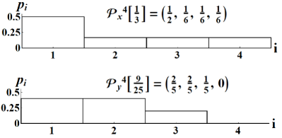
Figure 1: Illustrations of distributions over four outcomes

$$(2-\alpha)H_{\alpha}(\textbf{S}_{g}|\rho)\leq(2-\alpha)H_{\alpha}(\mathscr{P}_{x}^{d^{2}}\left[I(\textbf{S}_{g}|\rho)\right]),$$ (12)

$$(2-\alpha)H_{\alpha}(\textbf{S}_{g}|\rho)\geq(2-\alpha)H_{\alpha}(\mathscr{P}_{y}^{d^{2}}\left[I(\textbf{S}_{g}|\rho)\right]),$$ (13)

where $IC(\textbf{S}_{g}|\rho)$ is given by (6). This is the best result that can be obtained based on (6) only, hence uncertainty relations constructed from (6) such as those proposed in Ref. Raste ; indexofgsic cannot be stronger than our results. In the case $\alpha\to\infty$, Eq. (12) reduces to the result proposed previously by Rastegin indexofgsic ,

$$H_{\infty}(\textbf{S}_{g}|\rho)$$

$$\geq 2\log_{2}d-\log_{2}\Big{[}1+\sqrt{ad^{3}-1}\sqrt{Tr(\rho^{2})d-1}\Big{]}.$$ (14)

Now we show (12) and (13) are tight respectively when $Tr(\rho^{2})\in[\frac{1}{d},d^{2}a]$ and $Tr(\rho^{2})\in[\frac{1}{d},\frac{d-2+ad^{2}}{(d-1)^{2}}]$. We only need to show the probability distributions $\mathscr{P}_{y/x}^{d^{2}}\left[I(\textbf{S}_{g}|\rho)\right]$ can be achieved by some positive semi definite matrix in the form $\rho=\sum_{i}x_{i}S_{i}$, where $x_{i}=\frac{d(da-1)+d(d^{2}-1)p_{i}}{d^{3}a-1}$ is the solution to $Tr(\rho)=1$ and $Tr(\rho S_{i})=p_{i}\in\mathscr{P}_{y/x}^{d^{2}}\left[I(\textbf{S}_{g}|\rho)\right]$. For (12), when $Tr(\rho^{2})\leq d^{2}a$ we have $x_{1}\geq x_{2}=\cdots=x_{d^{2}}\geq 0$, obviously $\rho\geq 0$. As for (13), we have $x_{1}=\cdots=x_{d^{2}-1}\geq x_{d^{2}}$, as $\sum_{i}S_{i}={\bf 1}_{d}$, then $\forall|\phi\rangle\in\mathcal{H}_{d}$, $\langle\phi|\rho|\phi\rangle=\langle\phi|\sum_{i}x_{i}S_{i}|\phi\rangle=x_{1}+(x_{d^{2}}-x_{1})Tr(S_{d^{2}}|\phi\rangle\langle\phi|)\geq x_{1}+(x_{d^{2}}-x_{1})/d\geq 0$, thus $\rho$ is a density matrix.

By random sampling over density matrices on $\mathcal{H}_{3}$,

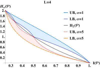
Figure 2: Information diagrams of Shannon entropy and Rényi 5-entropy (see also Refs. J3 ; HT ).

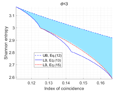
Figure 3: Information diagram of Shannon entropy for SIC-POVM on $\mathcal{H}_{3}$ (cyan region).

we obtain the information diagram shown in Fig. 3. It is not a surprise to see that our entropic lower bound for SIC-POVM is not tight when $Tr(\rho^{2})>\frac{1}{2}$ since (12) and (13) are based on Eq. (6) only. Interestingly, the corresponding tight bound agrees with

$$H(\textbf{S}_{g}|\rho)\geq H\big{(}\mathscr{P}_{y}^{4}[2I(\textbf{S}_{g}|\rho)]\big{)}+1.$$ (15)

IV Uncertainty relations for MUMs

IV.1 Rényi entropy with $\alpha\leq 1$

We show Theorem 2 in Appendix C.

Theorem 2. The sum of Shannon entropies for a finite set P of $|{\bf P}|$ MUMs with efficiency parameter $\kappa$ and performed on an arbitrary $d$-dimensional system $\rho$ is bounded from below by

$$H(\mathscr{P}_{y}^{d}[c])+k\log_{2}n+(|\textbf{P}|-k-1)\log_{2}(n+1),$$ (16)

with $C(\textbf{P}|\rho)=\frac{|\textbf{P}|}{d}+\frac{\kappa d-1}{d(d-1)}\left[dTr(\rho^{2})-1\right]$, here $n=\lfloor\frac{|\textbf{P}|}{C(\textbf{P}|\rho)}\rfloor$, $k=\lfloor(C(\textbf{P}|\rho)-\frac{M}{n+1})(n+1)n\rfloor$, and $c=C(\textbf{P}|\rho)-\frac{k}{n}-\frac{|\textbf{P}|-k-1}{n+1}$.

Despite the complex expression, this theorem can be understood in a simple way as is discussed in Appendix C. When $Tr(\rho^{2})\in[\frac{1}{d},\frac{d+\kappa-2}{(d-1)^{2}}]$, (16) reduces to

$$(|\textbf{P}|-1)\log_{2}d+H\big{(}\mathscr{P}_{y}^{d}\big{[}C(\textbf{P}|\rho)-(|\textbf{P}|-1)/d\big{]}\big{)},$$ (17)

which is actually valid for arbitrary Rényi $\alpha$-entropy with $0<\alpha\leq 1$, and quite similar to (12) it is tight.

We can linearize the first term of Eq.(16) based on its concavity with respect to $c$ as follows:
$H(\mathscr{P}_{y}^{d}[c])\geq H(\mathscr{P}_{y}^{d}[\frac{1}{n+1}])$
$+n(n+1)(c-\frac{1}{n+1})\left[H(\mathscr{P}_{y}^{d}[\frac{1}{n}])-H(\mathscr{P}_{y}^{d}[\frac{1}{n+1}])\right]$, which would then reduce to the result of Wu et al. WYM for MUBs,

$$H({\bf B}|\rho)\geq \left[|\textbf{B}|-nC(\textbf{B}|\rho)\right](n+1)\log_{2}(n+1)$$

$$- [|\textbf{B}|-(n+1)C(\textbf{B}|\rho)]n\log_{2}n,$$ (18)

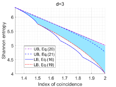
Figure 4: Information diagram of Shannon entropy for complete MUBs in $\mathcal{H}_{3}$.

where $C(\textbf{B}|\rho)$ is given by the right hand side of (7) and $n=\lfloor\frac{|\textbf{B}|}{C(\textbf{B}|\rho)}\rfloor$. (16) is generally improved from (18) and they are equivalent only when $c=\frac{1}{n}$ or $\frac{1}{n+1}$.

As can be seen in Fig. 4, similar to (13), (16) is not tight when $Tr(\rho^{2})>\frac{1}{2}$ for $d=3$ and the tight lower bound seems to be

$$H(\textbf{B}|\rho)\geq 1+3H\big{(}\mathscr{P}_{y}^{3}[\frac{1+Tr(\rho^{2})}{3}]\big{)}.$$ (19)

As for the upper bound, with $L=d$ we only propose the following two unproved approximations

$$(d+1)H\big{(}\mathscr{P}_{x}^{d}[I(\textbf{B}|\rho)/(d+1)]\big{)},\hskip 3.99994pt\text{$Tr(\rho^{2})\approx 1$}$$ (20)

$$d\log_{2}d+H(\mathscr{P}_{x}^{d}\left[I(\textbf{B}|\rho)-1\right]),\hskip 6.00006ptTr(\rho^{2})\approx\frac{1}{d}$$ (21)

IV.2 Rényi entropy with $\alpha\geq 2$

Theorem 3. Let P be a set of mutually unbiased measurements performed on a $d$-dimensional system $\rho$, then for any $\alpha\geq 2$

$$\frac{1}{|\textbf{P}|}H_{\alpha}({\bf P}|\rho)\geq\frac{\alpha}{1-\alpha}\log_{2}p_{a}+$$

$$\frac{\log_{2}d}{(1-\alpha)\ln[1+(d-1)^{\frac{2}{\alpha}}]}\ln\left[1+(d-1)^{\frac{2}{\alpha}}\frac{p_{b}^{2}}{p_{a}^{2}}\right],$$ (22)

where $p_{a}=\frac{1+\sqrt{(d-1)(dc-1)}}{d}$, $p_{b}=\frac{1-\sqrt{(dc-1)/(d-1)}}{d}$, and with $C(\textbf{P}|\rho)$ being the right hand side of Eq. (8), $c=\frac{1}{|\textbf{P}|}C(\textbf{P}|\rho)$.

This inequality is a direct result of the fact that the right hand side of (22) is convex with respect to $c$. When $\alpha>2$, Eq. (22) is improved from Rastegin’s lower bounds $L_{Ras1}$ Raste and $L_{Ras2}$ design2

$$\left\{\begin{aligned} &L_{Ras1}=\frac{\alpha}{2(1-\alpha)}\log_{2}c\\ &L_{Ras2}=\frac{\alpha-2}{1-\alpha}\log_{2}\Big{(}\frac{1+\sqrt{(dc-1)(d-1)}}{d}\Big{)}\\ +&\frac{1}{1-\alpha}\log_{2}c,\end{aligned}\right.$$ (23)

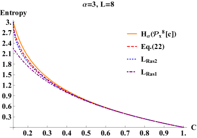
Figure 5: Lower bound on Rényi-3 entropy of a single probability distribution.

and when $\alpha=2$ they all reduce to $-\log_{2}c$. A comparison between these results when $\alpha=3$ and $L=8$ is shown in Fig. 5

IV.3 Entropy region

The entropies of performing a finite ordered set of generalized measurements $\textbf{P}=\{\mathcal{P}^{m}\}$ on a $d$-dimensional system described by $\rho$ form an vector, the $m{th}$ element of which is $H(\mathcal{P}^{m}|\rho)$. The region of all possible entropic vectors induced by P is called the entropy region of P. The entropy region of a given measurement set contains much more information besides the entropic lower bound, and we expect it to be as meaningful in quantum information theory as in the classical counterpart.

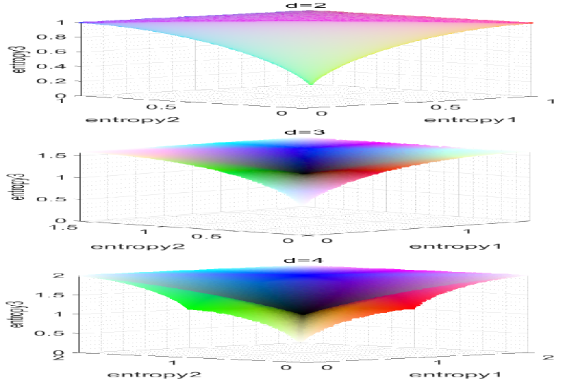
(a) Shannon entropy region for three MUBs.

(b) Shannon entropy region of three probability distributions satisfying Eq. (24)

Figure 6: Shannon entropy regions for three MUBs

We make a comparison here between the Shannon entropy region for three MUBs in $\mathcal{H}_{d}$ and that of three probability distributions over $d$ outcomes satisfying

$$\frac{3}{d}\leq\sum_{m=1}^{3}I(\mathscr{P}^{m})\leq\max\limits_{\rho}\{I(\textbf{B}|\rho)\}=1+\frac{2}{d}$$ (24)

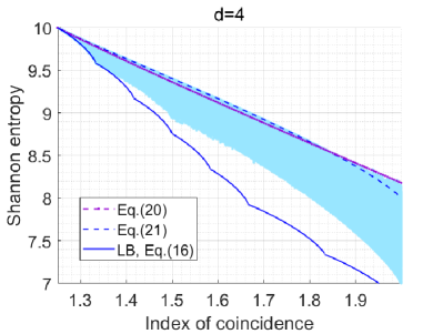
Figure 7: Information diagram of Shannon entropy for complete MUBs in $\mathcal{H}_{4}$.

As can be seen in Fig. 6, the entropy region of probability distributions satisfying Eq. (24) is the same to that for three MUBs when $d=2$, while in higher dimensions distinctions show up at places where the sum of entropies is relatively small, which is in accordance with the information diagrams.

V Discussions

We can see from Figs. (3,4, and 7) that the tight lower Rényi entropic ($\alpha<2$) bound curves for both complete MUBs and SIC-POVMs are non-differentiable at $Tr(\rho^{2})=\frac{1}{k}$ $(\forall k=2,\cdots,d-1)$, which divide the curves into $d-1$ sections. A natural thought is that different sections corresponds with density matrices at different boundaries of the set of positive semi-definite Hermitian matrices, namely, different sections of the lower bound curve are attained by density matrices of different ranks.

Conjecture. The tight lower bound on Shannon entropy for complete MUBs or SIC-POVMs on $\mathcal{H}_{d}$ can only be achieved by density matrices satisfying $(\lambda_{1},\lambda_{2},\cdots)=\mathscr{P}_{y}^{d}[Tr(\rho^{2})]$, where $\{\lambda_{i}\}$ are nonzero eigenvalues of $\rho$ and arranged in descending order.

We believe this conjecture, if confirmed, will be helpful in searching for tight state-independent EURs for complete MUBs and SIC-POVMs, which could be more efficient in applications of quantum information theory.

Based on the conjecture above, we have an alternative form of Eq. (16) for MUBs when $Tr(\rho^{2})\leq\frac{1}{d-1}$

$$H({\bf B}|\rho)\geq(|\textbf{B}|-1)\log_{2}d-Tr[\rho\log_{2}\rho],$$ (25)

which coincides with the uncertainty relation for two observables proposed by Berta et al. berta .

Lastly, we show an application of entropic uncertainty relations in entanglement detection. Let $\rho_{AB}=\sum_{i}p_{i}\rho_{i}^{A}\otimes\rho_{i}^{B}$ be an arbitrary separable state on the bipartite Hilbert space $\mathcal{H}_{A}\otimes\mathcal{H}_{B}$, and $\rho_{A}=Tr_{B}(\rho_{AB})$ and $\rho_{B}=Tr_{A}(\rho_{AB})$ are the reduced density matrices. According to the results shown in Ref. entangle2 , for any nondegenerate observables $\{A_{1},A_{2},\cdots\}$ on $\mathcal{H}_{A}$ and $\{B_{1},B_{2},\cdots\}$ on $\mathcal{H}_{B}$, there is

$$\sum_{m}H_{\alpha} \big{(}\mathscr{P}(A_{m}\otimes B_{m}|\rho_{AB})\big{)}\geq D=\max\{D_{A},D_{B}\},$$

where $$D_{A}=\sum_{m}H_{\alpha}\big{(}\mathscr{P}(A_{m}|\rho_{A})\Big{)},$$ (26)

$$D_{B}=\sum_{m}H_{\alpha}\big{(}\mathscr{P}(B_{m}|\rho_{B})\big{)}.\hskip 5.0pt(\alpha>0)$$

Here, $\mathscr{P}(A_{m}\otimes B_{m}|\rho_{AB})$ is the probability distribution induced by measuring $A_{m}\otimes B_{m}$ on $\rho_{AB}$, and $\mathscr{P}(A_{m}|\rho_{A})$ and $\mathscr{P}(B_{m}|\rho_{B})$ are the two corresponding marginal probability distributions.

Any bipartite state violating Eq. (26) must be entangled. When $\{A_{m}\}$ and $\{B_{m}\}$ are complementary observables, $D$ is the sum of entropies for measuring $\rho_{A}$ or $\rho_{B}$ in MUBs. According to our uncertainty relations in the previous section, a further lower bound for $D$ can be obtained directly from (22) when $\alpha\geq 2$ and from (16) when $\alpha=1$.

As an example, consider a pair of qudits in a Werner state $\mathcal{W}_{AB}=\frac{1-p}{d^{2}}{\bf 1}_{d^{2}}+p|\psi\rangle\langle\psi|$ $(0\leq p\leq 1)$, where $|\psi\rangle=\frac{1}{\sqrt{d}}(|0\rangle\otimes|0\rangle+\cdots+|d-1\rangle\otimes|d-1\rangle)$, and $\{\sigma_{m}\}$ ($m=1,2,\cdots,M)$ is a set of complementary observables in $\mathcal{H}_{d}$. The density matrix of a single qudit is then $\mathcal{W}_{A}=\mathcal{W}_{B}=\frac{1}{d}{\bf 1}_{d}$, which is independent of $p$. For simplicity, suppose now $d$ is a prime power and $M=d+1$, in which case $D=(d+1)\log_{2}d$ is state-independent, and moreover, the strongest form of (26) becomes

$$\sum_{m}^{d+1}H_{\infty}\big{(}\mathscr{P}(\sigma_{m}\otimes\sigma_{m}|\mathcal{W}_{AB})\big{)}\geq(d+1)\log_{2}d$$ (27)

since Rényi $\alpha$-entropy is a non-increasing function of $\alpha$. Numerical results show that (27) can be violated for $p>0.33$ when $d=2$ and for $p>0.46$ when $d=3$. As the bipartite Werner state is entangled if and only if $p>\frac{1}{d+1}$ sep2 ; sep3 ; sep4 ; sep5 , Eq. (27) is strong enough when $d=2$ but it is not strong when $d=3$ and fails to detect all entangled states.

From the above example we know that our EURs can be used to detect entanglement, and more stronger separability criteria based on our uncertainty relations are also possible. More works on entropic separability criteria can be found in Refs. [11, 15, 23].

CONCLUSION

In this paper we have obtained improved entropic uncertainty relations for general symmetric informationally complete positive operator-valued measures and mutually unbiased measurements in terms of Rényi entropy, which are shown to be tight for sufficiently mixed states. It might be the first time that tight state-dependent entropic uncertainty relations for multiple generalized measurements have been obtained. By random sampling density matrices and calculating the corresponding entropy for a given set of measurements, comparisons between our entropic bounds and the numerical optimal bounds are made via information diagrams. Our investigation of entropic uncertainty relations could provide some insights for further applications of uncertainty relations in information theory.

Appendix A Proof of Theorem 1

We employ Lagrangian multiplier method to find the distributions which make Rényi $\alpha$-entropy attain local extreme values on the set: ${\bf S}(L,c)=\left\{\mathscr{P}|length(\mathscr{P})=L\geq 3,\hskip 5.0ptI(\mathscr{P})=c<1\right\}$.

$$L_{\alpha} =\sum_{i=1}^{L}{p_{i}}^{\alpha}+\lambda(\sum_{i=1}^{L}p_{i}^{2}-c)+\lambda^{\prime}(\sum_{i=1}^{L}p_{i}-1);$$

$$\frac{\partial{L_{\alpha}}}{\partial{p_{i}}} =\alpha p_{i}^{\alpha-1}+2\lambda p_{i}+\lambda^{\prime}=0,\hskip 5.0pt1\leq i\leq L.\hskip 10.00002pt(\alpha>0,\alpha\neq 1)$$ (28)

where $\lambda$ and $\lambda^{\prime}$ are multipliers. Note the equation $\alpha x^{\alpha-1}=-2\lambda x-\lambda^{\prime}x$ has at most two different solutions as $x^{\alpha-1}$ is either concave or convex with respect to $x$ and $-2\lambda x-\lambda^{\prime}x$ describes a line. But (28) is not valid if there exists $1\leq i\leq L$ such that $p_{i}=0$.

When $\alpha<1$ and $p_{i}\to 0$, in which case $p_{i}^{\alpha-1}\to+\infty$. This implies on ${\bf S}(L,c)$, Rényi $\alpha$-entropy can only attain local minimum value at probability distributions whose positive probabilities satisfy (28), and it can never attain local maximum value at a distribution the smallest probability in which is 0. When $\alpha>1$, $\frac{\partial}{\partial p_{i}}(\sum_{i}p_{i}^{2}-c)\big{|}_{p_{i}=0}=0$, again, (28) is a restriction on the positive probabilities only.

We only need to consider those distributions containing at most two different positive probabilities, $p_{a}$ and $p_{b}$ say, and let’s parameterize them with three parameters as follows: N, the number of positive probabilities; $N_{a}$, the number of probabilities being $p_{a}$; $c$, the index of coincidence. We arrange the positive probabilities in descending order and represent the distribution formally as

$$\mathscr{P}[c,N,N_{a}]=\Big{(}N_{a}\odot p_{a},(N-N_{a})\odot p_{b}\Big{)},\hskip 10.00002pt(1/N\leq c\leq 1/N_{a})$$ (29)

where $N_{a}\odot p_{a}$ is shorthand for $N_{a}$ probabilities being $p_{a}$. Combined with the condition that $N_{a}p_{a}+(N-N_{a})p_{b}=1$ and $I\big{(}\mathscr{P}[c,N,N_{a}]\big{)}=c$, we have $p_{a}=$ $\frac{1+\sqrt{(Nc-1)(N-N_{a})/N_{a}}}{N}$ and $p_{b}=\frac{1-\sqrt{(Nc-1)N_{a}/(N-N_{a})}}{N}$. It can be checked that $\mathscr{P}[c_{1},N,N_{a}]$ majorizes $\mathscr{P}[c_{2},N,N_{a}]$ if $c_{1}>c_{2}$, thus $H_{\alpha}(\mathscr{P}[c,N,N_{a}])$ is a decreasing function of $c$.

Given the values of $u$, $c$ $(1/N\leq c<\frac{1}{N_{a}})$, and $N$ ($N_{a}$), the values of $N_{a}$ $(N)$, $p_{a}$, and $p_{b}$, if exist, are uniquely determined by (30).

$$\left\{\begin{aligned} 0\leq p_{b}<p_{a},N\geq N_{a}\geq 1,0<\alpha\neq 2\hskip 5.0pt\text{and}\hskip 5.0pt\alpha\neq 1,\hskip 156.49014pt\\ N_{a}p_{a}+(N-N_{a})p_{b}=1;\hskip 10.00002ptN_{a}p_{a}^{2}+(N-N_{a})p_{b}^{2}=c;\hskip 10.00002ptN_{a}p_{a}^{\alpha}+(N-N_{a})p_{b}^{\alpha}=u>0.\\ \end{aligned}\right.$$ (30)

$$H_{\alpha}\big{(}\mathscr{P}[1/N+s,N,N_{a}]\big{)}=\log_{2}N-\frac{\alpha Ns}{2\ln 2}+\frac{\alpha(\alpha-2)N^{\frac{3}{2}}N_{a}s^{\frac{3}{2}}}{4\ln 2(N-N_{a})}+o(s^{2}),\hskip 10.00002pt(0<s\ll\frac{1}{N_{a}}-\frac{1}{N}).$$ (31)

Note that $H_{\alpha}\big{(}\mathscr{P}[\frac{1}{N},N,N_{a}]\big{)}=\log_{2}N$ is independent of $N_{a}$ and $\lim_{c\to 1/N_{a}}H_{\alpha}\big{(}\mathscr{P}[c,N,N_{a}]\big{)}=\log_{2}N_{a}$ is independent of $N$, thus $H_{\alpha}\big{(}\mathscr{P}[c,N,N_{a}]\big{)}$ is monotonic of $N$ if $c\neq\frac{1}{N}$ and monotonic of $N_{a}$ if $c\neq\frac{1}{N_{a}}$, more concretely, taking the series expansion of entropy (31) into consideration we have

$$(2-\alpha)H_{\alpha}\big{(}\mathscr{P}[c,N,N_{a}]\big{)}\geq(2-\alpha)H_{\alpha}\big{(}\mathscr{P}[c,N,N_{a}^{\prime}]\big{)},\hskip 5.0pt(N_{a}<N_{a}^{\prime},\frac{1}{N}\leq c\leq\frac{1}{N_{a}^{\prime}});$$ (32)

$$(2-\alpha)H_{\alpha}\big{(}\mathscr{P}[c,N,N_{a}]\big{)}\leq(2-\alpha)H_{\alpha}\big{(}\mathscr{P}[c,N^{\prime},N_{a}]\big{)},\hskip 5.0pt(N<N^{\prime},\frac{1}{N}\leq c\leq\frac{1}{N_{a}}).$$ (33)

We can conclude from (32) and (33) that for any distribution $\mathscr{P}$ over $L$ outcomes with $I(\mathscr{P})=c$ there is

$$(2-\alpha)H_{\alpha}\big{(}\mathscr{P}[c,L,1]\big{)}\geq(2-\alpha)H_{\alpha}\big{(}\mathscr{P}\big{)}\geq(2-\alpha)H_{\alpha}\big{(}\mathscr{P}[c,N,N-1]\big{)},$$ (34)

where $N$ is an integer such that $\frac{1}{L}\leq\frac{1}{N}\leq c<\frac{1}{N-1}$, namely, $N=\lceil\frac{1}{c}\rceil$. This completes the proof of Theorem 1.

Appendix B Properties of extreme values

Let’s reparametrize $\mathscr{P}[c,N,N_{a}]$ as $\mathscr{P}^{*}[c,N,\theta]$, where $\theta=2\arccos\sqrt{N_{a}/N}$ and $\theta\in[0,\pi)$. We have

$$H_{\alpha}\big{(}\mathscr{P}^{*}[c,N,\theta]\big{)} =\frac{1}{1-\alpha}\log_{2}\Big{[}N\cos^{2}\frac{\theta}{2}\Big{(}\frac{1+\sqrt{Nc-1}\tan\frac{\theta}{2}}{N}\Big{)}^{\alpha}+N\sin^{2}\frac{\theta}{2}\Big{(}\frac{1-\sqrt{Nc-1}\cot\frac{\theta}{2}}{N}\Big{)}^{\alpha}\Big{]}$$

$$=\frac{1}{1-\alpha}\log_{2}M_{\alpha}(\mathscr{P}^{*}[c,N,\theta])$$

$$(\alpha-1)\frac{\partial^{2}}{\partial c^{2}}H_{\alpha}\big{(}\mathscr{P}^{*}[c,N,\theta]\big{)} =f(\alpha,z,\theta)\frac{\alpha N^{\alpha+1}\sin\frac{\theta}{2}\cos^{3}\frac{\theta}{2}}{4\ln 2(Nc-1)^{3/2}M_{\alpha}^{2}\big{(}\mathscr{P}^{*}[c,N,\theta]\big{)}}\left(1+\sqrt{Nc-1}\tan\frac{\theta}{2}\right)^{2\alpha-2}$$

where, with $z=\frac{1-\sqrt{Nc-1}\cot\frac{\theta}{2}}{1+\sqrt{Nc-1}\tan\frac{\theta}{2}}$ $(0<z\leq\tan\frac{\theta}{2})$, $f(\alpha,z,\theta)$

$$= \frac{2\tan^{2}\frac{\theta}{2}}{1+z\tan^{2}\frac{\theta}{2}}(z^{\alpha-1}-1)^{2}+z^{\alpha-1}\left[-\tan^{2}\frac{\theta}{2}z^{\alpha-1}+z^{1-\alpha}+(\alpha-1)(z\tan^{2}\frac{\theta}{2}-\frac{1}{z})+(2-\alpha)(\tan^{2}\frac{\theta}{2}-1)\right]$$

$$\geq z^{\alpha-1}\left[-\tan^{2}\frac{\theta}{2}z^{\alpha-1}+z^{1-\alpha}+(\alpha-1)(z\tan^{2}\frac{\theta}{2}-\frac{1}{z})+(2-\alpha)(\tan^{2}\frac{\theta}{2}-1)\right]$$

when $\alpha\in(0,1)\cup[2,+\infty)$ and $0<\tan\frac{\theta}{2}\leq 1$,

$$f(\alpha,z,\theta)\geq z^{\alpha-1}\left[-z^{\alpha-1}+z^{1-\alpha}+(\alpha-1)(z-\frac{1}{z})\right]\geq 0\Longrightarrow(\alpha-1)\frac{\partial^{2}}{\partial c^{2}}H_{\alpha}\big{(}\mathscr{P}^{*}[c,N,\theta]\big{)}\geq 0$$ (35)

As for Shannon entropy, when $0<z<\tan\frac{\theta}{2}\leq 1$

$$\frac{\partial^{2}}{\partial c^{2}}H\big{(}\mathscr{P}^{*}[c,N,\theta]\big{)}=\log_{2}(1+z\tan{\frac{\theta}{2}})-\log_{2}(1-z\cot{\frac{\theta}{2}})-\frac{1}{1-z\cot{\frac{\theta}{2}}}+\frac{1}{1+z\tan{\frac{\theta}{2}}}\leq 0.$$ (36)

(35) and (36) imply that when $N_{a}\in[N/2,N]$, $H_{\alpha}\big{(}\mathscr{P}[c,N,N_{a}]\big{)}$ is concave with respect to $c$ when $\alpha\leq 1$ and convex with respect to c when $\alpha\geq 2$.

Appendix C Proof of Theorem 2

Let g=$\{\mathscr{P}^{g}\}$ denote the probability distributions at which $\sum_{m=1}^{M}H(\mathscr{P}^{m})$ is minimum under the restriction

$$\forall 1\leq m\leq M,length(\mathscr{P}^{m})=L;\hskip 5.0pt\sum_{m=1}^{M}I(\mathscr{P}^{m})=\sum_{m}c^{m}=c\hskip 5.0pt\text{($c$ is a constant, $c\in[\frac{M}{d},M]$)},$$ (37)

where $\mathscr{P}^{g}$ is the $gth$ distribution in g. Firstly, according to (34) (or Theorem 1) and (36) we have the following
Property 1. $\mathscr{P}^{g}$ must be in the form $\mathscr{P}^{g}=\mathscr{P}_{y}^{L}[c^{g}]$ for any $g$.
Property 2. At most one element in g, $\mathscr{P}^{k}$ say, is not uniform in its nonzero part.
It can be proved that for any $2\leq m<n$ $(n,m\in N^{+})$,

$$\left\{\begin{aligned} 1.\hskip 5.0ptH\big{(}\mathscr{P}_{y}^{L}[1/n]\big{)}+H\big{(}\mathscr{P}_{y}^{L}[1/m+s]\big{)}>H\big{(}\mathscr{P}_{y}^{L}[1/m]\big{)}+H\big{(}\mathscr{P}_{y}^{L}[1/n+s]\big{)},\hskip 5.0pt0\leq s\leq 1/n/(n-1)\\ 2.\hskip 5.0ptH\big{(}\mathscr{P}_{y}^{L}[1/n-s]\big{)}+H\big{(}\mathscr{P}_{y}^{L}[1/m]\big{)}\geq H\big{(}\mathscr{P}_{y}^{L}[1/m-s]\big{)}+H\big{(}\mathscr{P}_{y}^{L}[1/n]\big{)},\hskip 5.0pt0\leq s\leq 1/n/(n+1)\end{aligned}\right.$$ (38)

$$\text{note here:}\hskip 5.0ptIC(\mathscr{P}_{y}^{L}[1/n])+IC(\mathscr{P}_{y}^{L}[1/m+s])=IC(\mathscr{P}_{y}^{L}[1/n+s])+IC(\mathscr{P}_{y}^{L}[1/m])$$

$$\hskip 50.00008ptIC(\mathscr{P}_{y}^{L}[1/n-s])+IC(\mathscr{P}_{y}^{L}[1/m])=IC(\mathscr{P}_{y}^{L}[1/m-s])+IC(\mathscr{P}_{y}^{L}[1/n]),$$

with $N_{g}$ denoting the number of nonzero probabilities of $\mathscr{P}^{g}$, a direct result of properties 1-2 and (38) is the following
$\begin{aligned} \text{{\bf Property 3}}.\hskip 10.00002pt1.\hskip 5.0pt&\max\limits_{g,g^{\prime}}|\{N_{g}-N_{g^{\prime}}\}|\leq 1;\hskip 20.00003pt2.\hskip 5.0pt\text{if}\hskip 5.0ptN_{k}=\min\limits_{g}\{N_{g}\},\hskip 5.0pt\text{then}\hskip 5.0pt\forall g,N_{g}-N_{k}=0\end{aligned}$
With Properties 1-3, it’s enough to determine g (Theorem 2). To show the first inequality of (38) we only need to show $\log_{2}N-H\big{(}\mathscr{P}_{y}[1/N+s,N,N-1]\big{)}$ is an increasing function of N. Under the parametrization introduced in Appendix B we have,

$$\log_{2}N-H\big{(}\mathscr{P}^{*}[1/N+s,N,\theta]\big{)}=\cos^{2}\frac{\theta}{2}\Big{(}1+\sqrt{Ns}\tan\frac{\theta}{2}\Big{)}\log_{2}\Big{[}\cos^{2}\frac{\theta}{2}\Big{(}1+\sqrt{Ns}\tan\frac{\theta}{2}\Big{)}\Big{]}$$ (39)

$$\sin^{2}\frac{\theta}{2}\Big{(}1-\sqrt{Ns}\cot\frac{\theta}{2}\Big{)}\log_{2}\Big{[}\sin^{2}\frac{\theta}{2}\Big{(}1-\sqrt{Ns}\cot\frac{\theta}{2}\Big{)}\Big{]}=h\big{(}s,N,\theta\big{)}$$

Let $\theta_{y}(N)=2\arctan\frac{1}{\sqrt{N-1}}$, then $\mathscr{P}[c,N,N-1]=\mathscr{P}^{*}[c,N,\theta_{y}(N)]$,

$$\frac{\partial}{\partial N}h\big{(}s,N,\theta\big{)}=\frac{s}{N}\frac{\partial}{\partial s}h\big{(}s,N,\theta\big{)}>0,\hskip 5.0pt\frac{\partial}{\partial\theta}h\big{(}s,N,\theta\big{)}<0,\hskip 5.0pt\frac{d\theta_{y}}{dN}<0$$

$$\frac{\partial}{\partial N}h\big{(}s,N,\theta_{y}(N)\big{)}=\Big{[}\frac{\partial}{\partial N}h\big{(}s,N,\theta\big{)}+\frac{\partial}{\partial\theta}h\big{(}s,N,\theta\big{)}\frac{d\theta_{y}}{dN}\Big{]}\Big{|}_{\theta=\theta_{y}(N)}\geq 0$$ (40)

Hence $h(s,N,\theta_{y}(N))$ is an increasing function of N, and the second inequality of (38) can be proved similarly.

It turns out that g is also the set of probability distributions that descends entropy the fastest locally. Consider $c=\frac{M}{L}$ (this is when probability distributions are all uniform) in the beginning and then let $c$ increase, then according to Properties 1, 2 and (31) obviously the steepest descent of Shannon entropy is given by

$$\left.\begin{aligned} &\Big{\{}(M-1)\odot\mathscr{P}_{y}^{L}\big{[}\frac{1}{L}\big{]},\mathscr{P}_{y}^{L}\big{[}c-\frac{M-1}{L}\big{]}\Big{\}},\hskip 90.00014pt\frac{M}{L}\leq c\leq\frac{M-1}{L}+\frac{1}{L-1}\\ &\Big{\{}(M-2)\odot\mathscr{P}_{y}^{L}\big{[}\frac{1}{L}\big{]},\mathscr{P}_{y}^{L}\big{[}\frac{1}{L-1}\big{]},\mathscr{P}_{y}^{L}\big{[}c-\frac{M-2}{L}-\frac{1}{L-1}\big{]}\Big{\}},\frac{M-1}{L}+\frac{1}{L-1}\leq c\leq\frac{M-2}{L}+\frac{2}{L-1}\\ &\hskip 40.00006pt\cdots\cdots\\ &\Big{\{}(M-1)\odot\mathscr{P}_{y}^{L}\big{[}\frac{1}{L-1}\big{]},\mathscr{P}_{y}^{L}\big{[}c-\frac{M-1}{L-1}\big{]}\Big{\}},\hskip 75.0001pt\frac{M}{L-1}\leq c\leq\frac{M-1}{L-1}+\frac{1}{L-2}\\ &\hskip 40.00006pt\cdots\cdots\end{aligned}\right\}={\bf g}$$

where $M\odot\mathscr{P}$ is shorthand for $M$ probability distributions being $\mathscr{P}$.

References

- (1) W. Heisenberg, Z. Phys. 43, 172 (1927).
- (2) H. P. Robertson, Phys. Rev. 34, 163 (1929).
- (3) D. Deutsch, Phys. Rev. Lett. 50, 631 (1983).
- (4) L. Dammeier, R. Schwonnek, and R. F. Werner, New J. Phys. 17, 093046 (2015).
- (5) I. Białynicki-Birula, and Ł. Rudnicki, 2011, in Statistical Complexity, edited by K. Sen (Springer Netherlands, Dordrecht), pp. 1-34
- (6) P. J. Coles, R. Colbeck, L. Yu, and M. Zwolak, Phys. Rev. Lett. 108, 210405 (2012).
- (7) S. Friedland, V. Gheorghiu, and G. Gour, Phys. Rev. Lett. 111, 230401 (2013).
- (8) J. B. M. Uffink and J. Hilgevoord, Found. Phys. 15, 925 (1985).
- (9) G. Vallone, D. G. Marangon, M. Tomasin, and P. Villoresi, Phys. Rev. A 90, 052327 (2014).
- (10) V. Giovannetti, Phys. Rev. A 70, 012102 (2004).
- (11) O. Gühne, and M. Lewenstein, Phys. Rev. A 70, 022316 (2004).
- (12) Yichen Huang, Phys. Rev. A 82, 012335 (2010).
- (13) R. König, S. Wehner, and J. Wullschleger, IEEE Trans. Inf. Theory 58, 1962 (2012).
- (14) F. Dupuis, O. Fawzi, and S. Wehner, IEEE Trans. Inf. Theory 61, 1093 (2015).
- (15) P. J. Coles, M. Berta, M. Tomamichel, and S. Wehner, Rev. Mod. Phys. 89, 015002 (2017).
- (16) K. Kraus, Phys. Rev. D 35 3070 (1987).
- (17) H. Maassen and J. B. M. Uffink, Phys. Rev. Lett. 60, 1103 (1988).
- (18) I. D. Ivonovic, J. Phys. A 25, L363 (1992).
- (19) J. Sánchez, Phys, Lett. A 173, 233 (1993).
- (20) J. Sánchez-Ruiz, Phys, Lett. A 201, 125 (1995).
- (21) M. A. Ballester and S. Wehner, Phys. Rev. A 75, 022319 (2007).
- (22) S. Wehner, and A. Winter, New J. Phys. 12, 025009 (2010).
- (23) S. Wu, S. Yu, and K. Mølmer, Phys. Rev. A 79, 022104 (2009).
- (24) I. Bengtsson et al., J. Math. Phys. 48, 052106 (2007).
- (25) J. M. Renes, R. Blume-Kohout, A. J. Scott, and C. M. Caves, J. Math. Phys. 45 2171 (2004).
- (26) A. Kalev and G. Gour, New J. Phys. 16, 053038 (2014).
- (27) G. Gour G and A. Kalev, J. Phys. A: Math. Theor. 47 335302 (2014).
- (28) A. E. Rastegin, Eur. Phys. J. D 67, 269 (2013).
- (29) A. E. Rastegin, Phys. Scr. 89, 085101 (2014).
- (30) B. Chen, and S. Fei, Quantum Inf. Process. 14, 2227-2238 (2015).
- (31) K. Wang, N. Wu, and F. Song, Phys. Rev. A 98, 032329 (2018).
- (32) A. Ketterer and O. Gühne, Phys. Rev. Research 2, 023130 (2020).
- (33) A. E. Rastegin, J. Phys. A: Math. Theor., Vol. 53, 405301 (2020).
- (34) A. Rényi, 1961, in Proceedings of the 4th Berkeley Symposium on Mathematical Statistics and Probability, Vol. 1 (University of California Press, Berkeley, CA), pp. 547-561.
- (35) P. Harremoës and F. Topsøe, IEEE Trans. Inf. Theory 47, 2944 (2001).
- (36) A. J. Scott, M. Grassl, J. Math. Phys. 51, 042203 (2010).
- (37) D. M. Appleby, Opt. Spectrosc. 103, 416-428 (2007).
- (38) A. Kalev, J. Phys. A: Math. Theor. 47 265301 (2014).
- (39) I. D. Ivonovic, J. Phys. A 14, 3241 (1981).
- (40) W. K. Wootters and B. D. Fields, Ann. Phys. (N.Y.) 191, 363 (1989).
- (41) A. Klappenecker and M. Rötteler, Finite Fields and Applications (Springer, Berlin-Heidelberg, 2004), pp. 137-144.
- (42) A. O. Pittenger and M. H. Rubin, Linear Algebr. Appl. 390, 255 (2004).
- (43) M. Berta, M. Christandl, R. Colbeck, J. M. Renes, and R. Renner, Nat. Phys. 6, 659 (2010).
- (44) A. O. Pittenger and M. H. Rubin Phys. Rev. A 62, 032313 (2000).
- (45) P. Rungta, W. J. Munro, K. Nemoto, P. Deuar, G. J. Milburn, and C. M. Caves, in Directions in Quantum Optics, Vol.561, edited by H. J. Carmichael, R. J. Glauber, and M. O. Scully (Springer-Verlag, Berlin-Heidelberg, 2001) pp. 149-164.
- (46) A. Peres, Phys. Rev. Lett. 77, 1413 (1996).
- (47) A. O. Pittenger, M. H. Rubin, Opt. Commun. 179, 447-449 (2000).