Duality for optimal consumption with randomly terminating income

Abstract.

We establish a rigorous duality theory, under No Unbounded Profit with Bounded Risk, for an infinite horizon problem of optimal consumption in the presence of an income stream that can terminate randomly at an exponentially distributed time, independent of the asset prices. We thus close a duality gap encountered by Vellekoop and Davis (2009) in a version of this problem in a Black-Scholes market. Many of the classical tenets of duality theory hold, with the notable exception that marginal utility at zero initial wealth is finite. We use as dual variables a class of supermartingale deflators such that deflated wealth plus cumulative deflated consumption in excess of income is a supermartingale. We show that the space of discounted local martingale deflators is dense in our dual domain, so that the dual problem can also be expressed as an infimum over the discounted local martingale deflators. We characterise the optimal wealth process, showing that optimal deflated wealth is a potential decaying to zero, while deflated wealth plus cumulative deflated consumption over income is a uniformly integrable martingale at the optimum. We apply the analysis to the Vellekoop and Davis (2009) example and give a numerical solution.

Dedicated to the memory of Mark H. A. Davis

MSC 2010 subject classifications: 93E20, 91G80, 91G10, 49M29, 49J55, 49K45

Keywords and phrases: Duality, utility from consumption, portfolio optimisation, supermartingale deflator, terminating income, HJB equation

1. Introduction

In this paper we establish a duality theory for an infinite horizon optimal consumption problem in which the agent also receives an income stream which terminates at a random exponentially distributed time, independent of the filtration governing the evolution of the asset prices. Such a problem was considered by Vellekoop and Davis (2009) in a Black-Scholes market. Here, we consider a general semimartingale incomplete market, under the minimal no-arbitrage assumption of no unbounded profit with bounded risk (NUPBR). We thus assume only the existence of a suitable class of deflators, and use no arguments involving equivalent local martingale measures (ELMMs). This is natural under NUPBR, and also desirable in a perpetual model, since ELMMs do not typically exist over infinite horizons.

In Vellekoop and Davis (2009), despite the apparent simplicity of the modification of the classical Merton problem with deterministic (or indeed no) income, the problem proved a remarkably intractable one to solve and understand. Vellekoop and Davis (2009) implemented a differential equation-based dual approach, made an ansatz that the dual control was deterministic, and used differential equation heuristics to argue that the derivative of the value function at zero initial wealth was infinite. Ultimately, though, they encountered a duality gap, in that their derived value function could not solve the Hamilton-Jacobi-Bellman (HJB) equation, indicating that the dual optimiser must indeed be stochastic and state-dependent in some way. What is more, their numerical solutions indicated that the value function derivative at zero initial wealth was finite. The intuition behind this last feature is clear: even though the income can terminate very soon after time zero, it cannot terminate immediately, except in the limiting case that the intensity of the exponential time approaches infinity. Thus, the agent is bound to receive some income, so is not infinitely penalised for having zero initial capital, and marginal utility of wealth is finite at this point.

The above issues make optimal consumption with randomly terminating income an open and interesting problem. We provide a dual characterisation of the problem in a general set-up, and close the duality gap. We find that most of the usual tenets of duality theory hold, with the exception that the marginal utility at zero initial wealth is indeed finite. We also characterise the optimal wealth process, and show that the optimal deflated wealth process is a potential, decaying almost surely to zero, while deflated wealth plus cumulative deflated consumption over income is a uniformly integrable martingale at the optimum. Our results apply also to the finite horizon version of the problem, both with and without a terminal wealth objective, and we describe the minor adjustments needed to do this in Section 5.4.

Our analysis is based on characterising the dual domain by a fundamental supermartingale property, using a class of deflators (consumption deflators) such that deflated wealth plus cumulative deflated consumption in excess of income is a supermartingale. The supermartingale property yields a budget constraint as a necessary condition (Lemma 2.1) for admissible consumption plans. Motivated by the budget constraint, we assume a financing condition (Assumption 2.3) that characterisies admissibility, so that the budget constraint is also a sufficient condition for admissibility. This ensures that the primal domain is closed in an appropriate topology. We show that our dual domain is closed and coincides with the closure (in an appropriate topology) of the discounted local martingale deflators (LMDs). But we are able to avoid having to explicitly invoke such a closure in defining our dual domain, which yields a stronger duality statement. This is discussed in Remark 2.4.

The mathematical contribution of the paper is to show how the seminal approach to convex duality for utility maximisation, as inspired by Kramkov and Schachermayer (1999, 2003) and recently adapted to the no-income infinite horizon consumption problem by Monoyios (2020), can be adapted to a problem with random endowment. The significant adaptations required by the presence of the income are that, first, the bipolar theorem of Brannath and Schachermayer (1999) is unavailable, becuase the primal variable appearing in the budget constraint is the difference between the consumption and income rates, so is not guaranteed to be non-negative, precluding an application of the bipolar theorem. Second, we do not enlarge the original dual domain of deflators to encompass all processes dominated by the deflators. This enlargement is typically carried out to reach the bipolar of the original dual domain. Not only is this not of use here, since the bipolar theorem is inapplicable, but the the presence of the random endowment renders the dual objective non-monotone in the dual variables, so the enlargement could result in the dual minimiser not coinciding with the minimiser in the enlarged domain. This is discussed in Remark 4.1.

The upshot of these features is that the important bipolarity result (Kramkov and Schachermayer, 1999, Proposition 3.1) that underpins classical duality has to be replaced by a suitable analogue. This is provided by Proposition 4.2, giving the key properties of the primal and dual domains in the abstract version of the problem. In particular, Proposition 4.2 states that the dual domain is closed, and bounded in $L^{1}(\mu)$ (with $\mu$ the measure in the abstract formulation of the problem). In the terminal wealth problem of Kramkov and Schachermayer (1999, 2003), the dual domain being bounded in $L^{1}(\mathbb{P})$ follows simply from the fact that the unit wealth process is admissible. Here, the argument is more subtle, and requires a strictly positive interest rate, which is natural in a perpetual consumption problem with income.

With Proposition 4.2 in place, some of the classical steps to a duality theorem can be brought to bear on the problem. We prove an abstract duality theorem (Theorem 4.3), from which the concrete duality (Theorem 3.1) follows, including a characterisation of the optimal wealth process, as well as the property of finite marginal utility at zero wealth. Note that other papers on utility from consumption with random endowment are not able to cover our model or to produce the corresponding results. In some papers, such as Karatzas and Žitković (2003) (or Cvitanić et al. (2001), with a terminal wealth objective), the models are finite horizon, under the No Free Lunch with Vanishing Risk (NFLVR) no-arbitrage assumption, so heavily reliant on ELMMs and the dual space is required to incorporate a singular part, in the form of finitely additive measures, so a unique dual optimiser of the form we obtain is elusive. In other papers, such as Hugonnier and Kramkov (2004); Mostovyi (2017); Mostovyi and Sîrbu (2020), finitely additive measures are avoided by expanding the dimension of the value function to incorporate an additional variable describing the number of units of the random endowment. These works are again over a finite horizon under NFLVR, so also reliant on ELMMs, and the expansion of dimension of the value function renders them unable to yield the sharp differentiability results we obtain for the value functions, only super-and sub-differential results. Some early papers on optimal investment and consumption with random endowment, usually in a Brownian filtration, adopt a HJB equation perspective, such as Duffie and Zariphopoulou (1993) and He and Pagès (1993), and do not cover our general model.

Finally, we analyse the Vellekoop and Davis (2009) example, exploring the ramifications of duality, and numerically solving the problem. By integrating over the distribution of the random income termination time, we transform the pre-income termination problem to a stochastic control problem with perpetual income in which utility is derived from consumption and inter-temporal wealth, and numerically solve the HJB equation for the resulting problem.

The remainder of the paper is structured as follows. In Section 2 we formulate the primal problem, budget constraint and the dual problem and outline the Vellekoop and Davis (2009) example. In Section 3 we state the main duality theorem (Theorem 3.1) and also Theorem 3.2, that the infima over consumption deflators and discounted local martingale deflators coincide. In Section 4 we state key properties of the abstract primal and dual domains (Proposition 4.2), the abstract duality theorem (Theorem 4.3) and the result (Proposition 4.4) which underlies Theorem 3.2. The proofs of these results are given in Section 5. In Section 6 we examine the Vellekoop and Davis (2009) example. Section 7 concludes.

2. Problem formulation

2.1. The financial market

We consider an infinite horizon investment-consumption problem in a semimartingale incomplete market, and in the presence of an income stream which terminates at an exponentially distributed time that is independent of the filtration governing the asset prices. We have a complete stochastic basis $(\Omega,\mathcal{F},\mathbb{F}:=(\mathcal{F}_{t})_{t\geq 0},\mathbb{P})$, with the filtration $\mathbb{F}$ satisfying the usual hypotheses of right-continuity and augmentation with $\mathbb{P}$-null sets of $\mathcal{F}$. The filtration $\mathbb{F}$ is given by

$$\mathbb{F}:=\mathbb{G}\vee\mathbb{F}^{N},$$

where $\mathbb{G}$ is the ($\mathbb{P}$-augmentation) of the filtration governing the evolution of a $d$-dimensional non-negative semimartingale stock price vector $S=(S^{1},\ldots,S^{d})$ and $\mathbb{F}^{N}$ is a filtration independent of $\mathbb{G}$, and is the augmentation of the filtration generated by the càdlàg process $N$, given by

(2.1) $$N_{t}:=\mathbbm{1}_{\{t<\tau\}},\quad t\geq 0,$$

where $\tau\sim\mathrm{Exp}(\eta)$ is an exponentially distributed time with parameter $\eta\geq 0$, independent of $\mathbb{G}$. The interest rate is a strictly positive $\mathbb{G}$-adapted process $r=(r_{t})_{t\geq 0}$ satisfying $\int_{0}^{t}r_{s}\,\mathrm{d}s<\infty,\,t\geq 0$. We assume that the interest rate is bounded below by a positive constant,

(2.2) $$r_{t}\geq\underline{r}>0,\quad\forall\,t\geq 0.$$

An agent with initial capital $x\in\mathbb{R}_{+}$ trades the stocks plus cash, consumes wealth at a non-negative adapted rate $c=(c_{t})_{t\geq 0}$, and receives income at some non-negative bounded adapted rate $f=(f_{t})_{t\geq 0}$. The consumption rate is assumed to almost surely satisfy the minimal integrability condition $\int_{0}^{t}c_{s}\,\mathrm{d}s<\infty,\,t\geq 0$.

The income stream is specified as follows. With $a=(a_{t})_{t\geq 0}$ a non-negative $\mathbb{G}$-adapted process, bounded above by some constant $\overline{a}>0$, we have a randomly terminating income stream, with $f$ given by

(2.3) $$f_{t}:=a_{t}N_{t}=a_{t}\mathbbm{1}_{\{t<\tau\}},\quad 0\leq a_{t}\leq\overline{a}<\infty,\quad t\geq 0.$$

Thus, the stochastic income stream pays at the bounded $\mathbb{G}$-adapted rate $a$ up to the random time $\tau$, at which point it abruptly terminates. The random termination of the income generates an additional source of market incompleteness above and beyond any inherent incompleteness in the original market in the absence of the income stream.

The agent’s trading strategy $H=(H^{1},\ldots,H^{d})$ is a predictable $S$-integrable process for the number of shares of each stock held. The agent’s wealth process, $X$, follows

(2.4) $$\,\mathrm{d}X_{t}=H_{t}\,\mathrm{d}S_{t}+r_{t}\left(X_{t}-H_{t}S_{t}\right)\,\mathrm{d}t-c_{t}\,\mathrm{d}t+f_{t}\,\mathrm{d}t,\quad X_{0}=x>0,$$

where for brevity we write $H_{t}\,\mathrm{d}S_{t}\equiv\sum_{i=1}^{d}H^{i}_{t}\,\mathrm{d}S^{i}_{t}$ and $H_{t}S_{t}\equiv\sum_{i=1}^{d}H^{i}_{t}S^{i}_{t}$.

For any process $P$, let $\widetilde{P}:=\exp\left(-\int_{0}^{\cdot}r_{s}\,\mathrm{d}s\right)P$ denote its discounted incarnation. In terms of discounted quantities, the wealth process has decomposition

(2.5) $$\widetilde{X}=\widetilde{X}^{0}+F-C,$$

where

(2.6) $$\widetilde{X}^{0}:=x+(H\cdot\widetilde{S})$$

is the discounted wealth process of a self-financing portfolio corresponding to strategy $H$, with $(H\cdot\widetilde{S})\equiv\int_{0}^{\cdot}H_{s}\,\mathrm{d}\widetilde{S}_{s}$ denoting the stochastic integral and $C:=\int_{0}^{\cdot}\widetilde{c}_{s}\,\mathrm{d}s,\,F:=\int_{0}^{\cdot}\widetilde{f}_{s}\,\mathrm{d}s$ denoting the non-decreasing cumulative discounted consumption and income processes.

As is known from Vellekoop and Davis (2009), because the income stream terminates randomly, the agent is not able to follow the classical program of borrowing against the present value of future income (so allowing wealth to become negative) and using the optimal no-income strategy with an initial wealth enlarged by the present value of future income. We shall therefore assume solvency at all times, so $X\geq 0$ almost surely in (2.4). In this case, for a given $x>0$, we call the pair $(H,c)$ (or $(X,c)$) an $x$-admissible investment-consumption strategy. Denote the $x$-admissible investment-consumption strategies by $\mathcal{H}(x)$:

(2.7) $$\mathcal{H}(x):=\left\{(H,c):\widetilde{X}:=x+(H\cdot\widetilde{S})+\int_{0}^{\cdot}(\widetilde{f}_{s}-\widetilde{c}_{s})\,\mathrm{d}s\geq 0,\,\mbox{a.s}\right\},\quad x>0.$$

With an abuse of terminology we shall sometimes refer to the wealth-consumption pair $(X,c)$ as an admissible investment-consumption pair, and we shall sometimes write $(X,c)\in\mathcal{H}(x)$ in place of $(H,c)\in\mathcal{H}(x)$. For $x=1$, we write $\mathcal{H}\equiv\mathcal{H}(1)$.

If, for a consumption process $c$ we can find a predictable $S$-integrable process $H$ such that $(H,c)\in\mathcal{H}(x)$ is an $x$-admissible investment-consumption strategy, then we say that $c$ is an $x$-admissible consumption process or, briefly, an admissible consumption plan. Denote the set of $x$-admissible consumption plans by $\mathcal{A}(x)$:

(2.8) $$\mathcal{A}(x):=\left\{c\geq 0:\exists\,H\,\mbox{such that}\,\widetilde{X}:=x+(H\cdot\widetilde{S})+\int_{0}^{\cdot}(\widetilde{f}_{s}-\widetilde{c}_{s})\,\mathrm{d}s\geq 0,\,\mbox{a.s}\right\},\quad x>0.$$

For $x=1$ we write $\mathcal{A}\equiv\mathcal{A}(1)$. It is easy to verify that $\mathcal{A}(x)$ is a convex set.

For $c\equiv f\equiv 0$, the wealth process is that of a self-financing portfolio, with discounted wealth process $\widetilde{X}^{0}$ as in (2.6). Define $\mathcal{X}(x)$ as the set of almost surely non-negative self-financing wealth processes with initial value $x>0$:

$$\mathcal{X}(x):=\left\{X^{0}:\widetilde{X}^{0}=x+(H\cdot\widetilde{S})\geq 0,\,\mbox{a.s.}\right\},\quad x>0.$$

We write $\mathcal{X}\equiv\mathcal{X}(1)$, with $\mathcal{X}(x)=x\mathcal{X}$ for $x>0$, and we note that $\mathcal{X}$ is a convex set.

Given the wealth decomposition in (2.5), an equivalent characterisation of the admissible consumption plans is that there exists a self-financing wealth process such that its discounted version plus cumulative discounted income dominates cumulative discounted consumption.

2.2. The primal problem

Let $U:\mathbb{R}_{+}\to\mathbb{R}$ be a utility function, strictly concave, strictly increasing, continuously differentiable on $\mathbb{R}_{+}$ and satisfying the Inada conditions

(2.9) $$\lim_{x\downarrow 0}U^{\prime}(x)=+\infty,\quad\lim_{x\to\infty}U^{\prime}(x)=0.$$

Let $\delta>0$ be an impatience factor for consumption. The optimisation problem we study is to maximise expected utility from consumption over the infinite horizon in the presence of the terminating income stream. The primal value function $u:\mathbb{R}_{+}\to\mathbb{R}$ is defined by

(2.10) $$u(x)=\sup_{c\in\mathcal{A}(x)}\mathbb{E}\left[\int_{0}^{\infty}U(c_{t})\,\mathrm{d}\kappa_{t}\right],\quad x>0,$$

where $\kappa:\mathbb{R}_{+}\to\mathbb{R}_{+}$ is discounted Lebesgue measure, given by

(2.11) $$\kappa_{0}=0,\quad\,\mathrm{d}\kappa_{t}=\mathrm{e}^{-\delta t}\,\mathrm{d}t.$$

For later use, define the positive process $\zeta=(\zeta_{t})_{t\geq 0}$ as the reciprocal of $(\,\mathrm{d}\kappa_{t}/\,\mathrm{d}t)_{t\geq 0}$:

(2.12) $$\zeta_{t}:=\left(\frac{\,\mathrm{d}\kappa_{t}}{\,\mathrm{d}t}\right)^{-1}=\exp\left(\delta t\right),\quad t\geq 0.$$

Our goal is to develop a rigorous dual characterisation of the problem in (2.10).

2.3. Deflators and the budget constraint

With the one-jump process $N$ in (2.1) we associate the non-negative càdlàg $(\mathbb{P},\mathbb{F})$-martingale $M$, defined by

(2.13) $$M_{t}:=N_{t}+\eta\int_{0}^{t}N_{s}\,\mathrm{d}s,\quad t\geq 0.$$

Let $Z^{\mathbb{G}}$ be a local martingale deflator for the asset market in the absence of the income stream. Denote the set of such deflators by $\mathcal{Z}^{\mathbb{G}}$. Each $Z^{\mathbb{G}}\in\mathcal{Z}^{\mathbb{G}}$ is a positive local martingale with unit initial value such that deflated discounted self-financing wealth $Z^{\mathbb{G}}\widetilde{X}^{0}$ is a local martingale, for each $X^{0}\in\mathcal{X}$.

Now incorporate the income stream, and let $\mathcal{Z}$ denote the set of local martingale deflators for the enlarged market, such that deflated discounted self-financing wealth is a local martingale. The set $\mathcal{Z}$ is then composed of positive local martingales $Z$ given by

(2.14) $$Z:=Z^{\mathbb{G}}\mathcal{E}(-\gamma\cdot M),$$

where $\mathcal{E}(\cdot)$ denotes the stochastic exponential, for càglàd adapted processes $\gamma$ satisfying $\gamma>-1,\,\gamma<+\infty$ almost surely. We note that as long as $\gamma<+\infty$, $\Gamma:=\mathcal{E}(-\gamma\cdot M)$ is a martingale.

The multiplicity of processes $Z\in\mathcal{Z}$ is the manifestation of the market incompleteness induced both by the inherent incompleteness of the asset market in the absence of the income, and also by the presence of the randomly terminating income. The latter source of incompleteness means that there is a multiplicity of integrands $\gamma$ in (2.14), as well as many processes $Z^{\mathbb{G}}\in\mathcal{Z}^{\mathbb{G}}$.

For each $Z\in\mathcal{Z}$ and $X^{0}\in\mathcal{X}$, the process $\widetilde{X}^{0}Z$ is a local martingale (and also a super-martingale), so the (convex) set $\mathcal{Z}$ is defined by

(2.15) $$\mathcal{Z}:=\left\{Z>0,\,\mbox{c\`{a}dl\`{a}g},\,Z_{0}=1:\mbox{$\widetilde{X}^{0}Z$ is a local martingale, for all $X^{0}\in\mathcal{X}$}\right\}.$$

For each $Z\in\mathcal{Z}$, we may define an associated supermartingale deflator as the discounted martingale deflator $\widetilde{Z}:=\exp\left(-\int_{0}^{\cdot}r_{s}\,\mathrm{d}s\right)Z,\,Z\in\mathcal{Z}$, and we denote the set of such supermartingales with initial value $y>0$ by $\widetilde{\mathcal{Y}}(y)$:

(2.16) $$\widetilde{\mathcal{Y}}(y):=\left\{Y:\mbox{$Y=y\widetilde{Z}=y\exp\left(-\int_{0}^{\cdot}r_{s}\,\mathrm{d}s\right)Z$, for $Z\in\mathcal{Z}$}\right\},\quad y>0.$$

We write $\widetilde{\mathcal{Y}}\equiv\widetilde{\mathcal{Y}}(1)$, with $\widetilde{\mathcal{Y}}(y)=y\widetilde{\mathcal{Y}}$ for $y>0$, and $\widetilde{\mathcal{Y}}$ is convex, inheriting this property from $\mathcal{Z}$.

Define a further set $\mathcal{Y}^{0}(y)$ of supermartingale deflators with initial value $y>0$ by

(2.17) $$\mathcal{Y}^{0}(y):=\left\{Y>0,\,\mbox{c\`{a}dl\`{a}g},\,Y_{0}=y:\mbox{$X^{0}Y$ is a supermartingale, for all $X^{0}\in\mathcal{X}$}\right\},\quad y>0.$$

As before, we write $\mathcal{Y}^{0}\equiv\mathcal{Y}^{0}(1)$, with $\mathcal{Y}^{0}(y)=y\mathcal{Y}^{0}$ for $y>0$. Clearly, the set $\mathcal{Y}^{0}$ is convex, and it includes all the processes in the set $\widetilde{\mathcal{Y}}$ of discounted local martingale deflators, but may include other processes. Since $X^{0}\equiv 1$ lies in $\mathcal{X}$ (one may choose to hold initial wealth without investing in stocks or the cash account), each $Y\in\mathcal{Y}^{0}$ is a supermartingale. We shall refer to $\mathcal{Y}^{0}$ as the set of supermartingale deflators, or as the set of wealth deflators. The processes $Y\in\mathcal{Y}^{0}$ correspond to the classical deflators defined by Kramkov and Schachermayer (1999, 2003) in their seminal treatment of the terminal wealth utility maximisation problem. We thus have the inclusion

(2.18) $$\mathcal{Y}^{0}\supseteq\widetilde{\mathcal{Y}}.$$

The no-arbitrage assumption implicit in our model,

(2.19) $$\mathcal{Y}^{0}(y)\neq\emptyset,$$

is tantamount to the NUPBR condition (see Karatzas and Kardaras (2007)). We shall work only with deflators, and will not require any arguments involving ELMMs. There are good reasons to do this. One is that ELMMs will typically not exist over the infinite horizon, even if local martingale deflators are martingales, because these martingales will not be uniformly integrable when considered over an infinite horizon (this is true even in the Black-Scholes model, see (Karatzas and Shreve, 1998, Section 1.7)). It is now well accepted, since the work of Karatzas and Kardaras (2007) (and was implicit in the seminal work of Karatzas et al. (1991), where ELMMs were not used) that the key ingredient for well-posed utility maximisation problems is the existence of a suitable class of deflators which act on primal variables to create supermartingales, and our approach is in this spirit.

2.3.1. Consumption deflators

We define the space which will form the dual domain for the consumption problem (2.10).

For $x>0$, let $(X,c)\in\mathcal{H}(x)$ be an admissible wealth-consumption pair, as defined in (2.7). Then $c\in\mathcal{A}(x)$ is an admissible consumption process, as defined in (2.8). The dual domain for the consumption problem (2.10) is defined by

(2.20) $$\mathcal{Y}(y):=\left\{Y>0,\,\mbox{c\`{a}dl\`{a}g},\,Y_{0}=y:\mbox{$XY+\int_{0}(c_{s}-f_{s})Y_{s}\,\mathrm{d}s$ is a supermartingale, $\forall\,c\in\mathcal{A}(x)$}\right\}.$$

As usual, we write $\mathcal{Y}\equiv\mathcal{Y}(1)$ and we have $\mathcal{Y}(y)=y\mathcal{Y}$ for $y>0$. The set $\mathcal{Y}$ is easily seen to be convex. We shall refer to the processes in the dual domain $\mathcal{Y}(y)$ as consumption deflators (or, simply, as deflators, when no confusion arises) to distinguish them from the corresponding wealth deflators $Y\in\mathcal{Y}^{0}(y)$ as defined in (2.17), when the consumption and income processes are absent (or are equal, so cancel out).

In (2.20), note that the wealth process $X$ is the one on the left-hand-side of (2.4), so incorporating consumption and income. Since $(X,c)\equiv(1,f)$ is an admissible consumption-investment pair, each $Y\in\mathcal{Y}(y)$ is a supermartingale. In particular, since $c\equiv f$ is an admissible consumption plan, and noting the decomposition in (2.5), the resulting wealth process $X=X^{0}$ is then self-financing. In this case we have that $XY=X^{0}Y$ is a supermartingale, so that $Y\in\mathcal{Y}(y)$ is also a wealth deflator as defined in (2.17). In other words, we have the inclusion

(2.21) $$\mathcal{Y}\subseteq\mathcal{Y}^{0}.$$

The dual domain $\mathcal{Y}(y),\,y>0$ for our utility maximisation problem (2.10) from inter-temporal consumption in the presence of the income stream is thus a specialisation of the one used by Kramkov and Schachermayer (1999, 2003) for the terminal wealth problem.

2.3.2. The budget constraint

The key to identifying the dual problem to (2.10) is a suitable budget constraint involving admissible consumption plans and some class of deflators. We show that such a budget constraint with consumption deflators, due to the defining supermnartingale property in (2.20). We later show that the same supermartingale property also holds with discounted local martingale deflators $Y\in\widetilde{\mathcal{Y}}$, so that the set of consumption deflators includes the set of discounted local martingale deflators.

In what follows we assume that $\mathbb{E}\left[\int_{0}^{\infty}f_{t}Y_{t}\,\mathrm{d}t\right]<\infty,\,\forall\,Y\in\mathcal{Y}$, that is, cumulative deflated income is integrable, and we note that this condition is indeed true, as we establish it later in Lemma 5.2.

Lemma 2.1 (Budget constraint).

For $x,y>0$, let $c\in\mathcal{A}(x)$ and $Y\in\mathcal{Y}(y)$. We then have the budget constraint

(2.22) $$\mathbb{E}\left[\int_{0}^{\infty}(c_{t}-f_{t})Y_{t}\,\mathrm{d}t\right]\leq xy,\quad x,y>0.$$

Proof.

The supermartingale property in (2.20) and the non-negativity of $XY$ imply that

$$\mathbb{E}\left[\int_{0}^{t}c_{s}Y_{s}\,\mathrm{d}s\right]\leq xy+\mathbb{E}\left[\int_{0}^{t}f_{s}Y_{s}\,\mathrm{d}s\right],\quad t\geq 0.$$

Letting $t\uparrow\infty$, using monotone convergence and re-arranging, we obtain (2.22).

∎

The set of consumption deflators includes the set of local martingale deflators, since the supermartingale property in (2.20) in fact holds with discounted local martingale deflators, as we now show, provided we assume that $\mathbb{E}\left[\int_{0}^{\infty}f_{t}Y_{t}\,\mathrm{d}t\right]<\infty,\,\forall\,Y\in\widetilde{\mathcal{Y}}$.

Lemma 2.2 (Budget constraint with discounted local martingale deflators).

Let $x,y>0$. For any $c\in\mathcal{A}(x)$ and $Y\in\widetilde{\mathcal{Y}}(y)$ we have the budget constraint

(2.23) $$\mathbb{E}\left[\int_{0}^{\infty}(c_{t}-f_{t})Y_{t}\,\mathrm{d}t\right]\leq xy,\quad x,y>0.$$

Proof.

For some fixed $y>0$, let $Y=y\widetilde{Z}\in\widetilde{\mathcal{Y}}(y)$ be a discounted local martingale deflator, as defined in (2.16). Recalling the wealth dynamics (2.4) and the discounted wealth decomposition (2.5), the Itô product rule applied to $XY=y\widetilde{X}Z$ yields

(2.24) $$XY+\int_{0}^{\cdot}(c_{s}-f_{s})Y_{s}\,\mathrm{d}s=xy+X^{0}Y+y\int_{0}^{\cdot}(F_{s-}-C_{s-})\,\mathrm{d}Z_{s},$$

where $X^{0}$ is the self-financing wealth process in the decomposition (2.5). We observe that the right-hand-side of (2.24) is a local martingale, since both $X^{0}Y=y\widetilde{X}^{0}Z$ and the integral with respect to $Z$ are local martingales.

For any $t\geq 0$ the random variable $\int_{0}^{t}f_{s}Y_{s}\,\mathrm{d}s$ is $\mathbb{P}$-integrable, since we have

$$\mathbb{E}\left[\int_{0}^{t}f_{s}Y_{s}\,\mathrm{d}s\right]\leq\overline{a}\int_{0}^{t}\mathbb{E}[Y_{s}]\,\mathrm{d}s<\infty,\quad t\geq 0.$$

Hence, the integrand on the left-hand-side of (2.24) is bounded below by an integrable random variable. Since $XY$ is non-negative, the right-hand side of (2.24) is a local martingale bounded below by an integrable random variable, so the Fatou lemma gives that

(2.25) $$\mbox{$XY+\int_{0}^{\cdot}(c_{s}-f_{s})Y_{s}\,\mathrm{d}s$ is a supermartingale, $\forall$ $c\in\mathcal{A}(x)$ and $Y\in\widetilde{\mathcal{Y}}(y)$}.$$

This supermartingale property then implies the budget constraint in (2.23) by the same argument as in the proof of Lemma 2.1.

∎

Since the supermartingale property in the defintion (2.20) also holds for discounted local martingale deflators (as in (2.25)), the set of consumption deflators contains the set of discounted local martingale deflators. We thus have the inclusion

(2.26) $$\mathcal{Y}\supseteq\widetilde{\mathcal{Y}}.$$

We observe that, combining (2.26) and (2.21), we have $\mathcal{Y}^{0}\supseteq\mathcal{Y}\supseteq\widetilde{\mathcal{Y}}$.

The budget constraint in (2.22) thus constitutes a necessary condition for admissible consumption plans. We assume that it in fact characterises admissible consumption plans, so is also a sufficient condition, by virtue of the following financing condition.

Assumption 2.3 (Financing condition).

For $x,y>0$, let $(X,c)\in\mathcal{H}(x)$ be any $x$-admissible wealth-consumption pair, so $c\in\mathcal{A}(x)$ is an admissible consumption plan, and let $Y\in\mathcal{Y}(y)$ be any consumption deflator. We assume that current wealth plus future income can finance future consumption, in the sense that

$$X_{t}Y_{t}+\mathbb{E}\left[\left.\int_{t}^{\infty}f_{s}Y_{s}\,\mathrm{d}s\right|\mathcal{F}_{t}\right]\geq\mathbb{E}\left[\left.\int_{t}^{\infty}c_{s}Y_{s}\,\mathrm{d}s\right|\mathcal{F}_{t}\right],\quad t\geq 0,$$

and that if (2.3) holds, then $c\in\mathcal{A}(x)$ and $(X,c)\in\mathcal{H}(x)$.

2.4. The dual problem

Let $V:\mathbb{R}_{+}\to\mathbb{R}$ denote the convex conjugate of the utility function $U(\cdot)$, defined by

$$V(y):=\sup_{x>0}[U(x)-xy],\quad y>0.$$

The map $y\mapsto V(y),\,y>0$, is strictly convex, strictly decreasing, continuously differentiable on $\mathbb{R}_{+}$, $-V(\cdot)$ satisfies the Inada conditions, we have the bi-dual relation $U(x):=\inf_{y>0}[V(y)+xy],\,x>0$, and $V^{\prime}(\cdot)=-I(\cdot)=-(U^{\prime})^{-1}(\cdot)$, where $I(\cdot)$ denotes the inverse of marginal utility. In particular, we have the inequality

(2.27) $$V(y)\geq U(x)-xy,\quad\forall\,x,y>0,\quad\mbox{with equality iff $U^{\prime}(x)=y$}.$$

The dual to the primal problem (2.10) is motivated in the usual manner with the aid of the budget constraint (2.22). For any $c\in\mathcal{A}(x),\,Y\in\mathcal{Y}(y)$ we have, on recalling the process $\zeta$ of (2.12) and (2.27), that

(2.28) $$\mathbb{E}\left[\int_{0}^{\infty}U(c_{t})\,\mathrm{d}\kappa_{t}\right] \leq \mathbb{E}\left[\int_{0}^{\infty}\left(V(\zeta_{t}Y_{t})+f_{t}\zeta_{t}Y_{t}\right)\,\mathrm{d}\kappa_{t}\right]+xy.$$

We therefore define the dual value function by

(2.29) $$v(y):=\inf_{Y\in\mathcal{Y}(y)}\mathbb{E}\left[\int_{0}^{\infty}\left(V(\zeta_{t}Y_{t})+f_{t}\zeta_{t}Y_{t}\right)\,\mathrm{d}\kappa_{t}\right],\quad y>0.$$

We shall assume throughout that the dual problem is finitely valued:

(2.30) $$v(y)<\infty,\quad\forall\,y>0.$$

It is well known that the condition (2.30) acts an alternative mild feasibility condition to the reasonable asymptotic elasticity condition of Kramkov and Schachermayer (1999) that ensures the usual tenets of a duality theory can hold, as detailed by Kramkov and Schachermayer (2003).

Remark 2.4 (Consumption deflators versus discounted LMDs).

Since the budget constraint holds for both consumption deflators $Y\in\mathcal{Y}$ and discounted local martingale deflators $Y\in\widetilde{\mathcal{Y}}\subseteq\mathcal{Y}$, a natural question to ask is whether the dual problem can be cast as a minimisation over discounted local martingale deflators. It turns out that this is possible provided one takes the closure of $\widetilde{\mathcal{Y}}$ with (with respect the topology of convergence in measure $\kappa\times\mathbb{P}$) as the dual domain. This is the content of Theorem 3.2, relying on the property that $\widetilde{\mathcal{Y}}$ is dense in $\mathcal{Y}$ (see Proposition 4.4).

The reason one must take the closure of $\widetilde{\mathcal{Y}}$ if basing the dual problem on local martingale deflators is that it seems hard to establish, in general, that $\widetilde{\mathcal{Y}}$ is a closed set. We shall prove that the dual domain $\mathcal{Y}$ is closed by exploiting results on so-called Fatou convergence of supermartingales. This is a primary reason for defining the dual domain in terms of a fundamental supermartingale criterion. This method of proof fails if using local martingale deflators, because the limiting supermartingale in the Fatou convergence method is known only to be a supermartingale, and not necessarily a local martingale deflator.

In our approach, we avoid the need to invoke a closure in defining the dual domain, yielding a stronger ultimate duality statement, and in some sense showing that we have identified the true space of dual supermartingales. This is more in the spirit of Kramkov and Schachermayer (1999, 2003). (As (Rogers, 2003, Important Remark, pp. 104–105) points out, having to invoke a closure in defining the dual domain weakens the statement of the final result somewhat.) Finally, the fact that we show that our dual domain actually coincides with the closure of the discounted local martingale deflators, completes the picture on this topic in a satisfying way.

2.5. The Davis-Vellekoop example

A canonical example of the primal problem (2.10) (and which motivated this paper) is provided by Vellekoop and Davis (2009). The underlying market is a Black-Scholes (BS) market with a single stock $S$ with constant market price of risk $\lambda\in\mathbb{R}$ and constant volatility $\sigma>0$, driven by a single Brownian motion $W$. The interest rate is a constant $r>0$, and the stock price dynamics are given by

$$\,\mathrm{d}S_{t}=(r+\sigma\lambda)S_{t}\,\mathrm{d}t+\sigma S_{t}\,\mathrm{d}W_{t}.$$

The income stream pays at a constant rate $a\geq 0$ until the random time $\tau\sim\mathrm{Exp}(\eta)$, so $f_{t}=aN_{t},\,t\geq 0$, with $N$ defined in (2.1) and $\tau$ independent of $W$. The underlying market in the absence of the income is thus complete, so all the incompleteness is generated by the random termination of the income. The filtration $\mathbb{G}$ is the $\mathbb{P}$-augmentation of the filtration generated by $W$, the unique martingale deflator in the absence of the income is $Z^{\mathbb{G}}=\mathcal{E}(-\lambda W)$, so the local martingale deflators in the market with the income are of the form

$$Z=\mathcal{E}(-\lambda W-\gamma\cdot M),\quad\gamma>-1,$$

with $M$ defined in (2.13). We take the filtration $\mathbb{F}$ to be the $\mathbb{P}$-augmentation of the filtration generated by $(W,N)$. Over any finite horizon, $Z$ is a martingale as long as $\gamma$ is finite. Over the infinite horizon it is well known that such a martingale is not uniformly integrable. This is the case even in the underlying BS market without the income stream, since the martingale $\mathcal{E}(-\lambda W)$ is not uniformly integrable over the infinite horizon, so ELMMs will not exist over the infinite horizon. Thus, even in this simple example, our approach of using deflators (as opposed to any constructions involving ELMMs) is a very natural one.

This example is remarkable in that, despite the apparent simplicity of the setting, the problem with randomly terminating income induces a particularly awkward form of market incompleteness. The agent is precluded from borrowing against the income stream, to avoid being left insolvent if the income terminates at a time when the wealth is negative. This raised many difficulties in Vellekoop and Davis (2009). First, there is no longer a closed form solution to the problem. Second, Vellekoop and Davis (2009) encountered a duality gap, as their conjectured primal solution, obtained by solving a deterministic control problem, could not solve the HJB equation. Finally, there was also an open question as to whether the marginal utility at zero wealth is finite or not. Economic intuition indicates that it should be finite as long as the income is strictly positive for a non-zero initial time interval, but ODE heuristics in Vellekoop and Davis (2009) seemed to suggest that the marginal utility at zero wealth was infinite, even though numerical solutions suggested the opposite conclusion.

For all the above reasons, the problem that Vellekoop and Davis (2009) came up with is a fascinating example, and we shall analyse it and give a numerical solution in Section 6, after first establishing a rigorous duality theory for the general semimartingale market model described earlier.

3. The duality theorem

Here is the main duality result of the paper (Theorem 3.1), a dual characterisation of the solution to the terminating income problem (2.10). Note that our methods also cover the finite horizon version of the problem, with or without a terminal wealth objective, and we give some remarks on the adjustments needed to do this after proving the theorem, in Section 5.4.

Theorem 3.1 (Consumption with randomly terminating income duality).

Define the primal value function $u(\cdot)$ by (2.10) and the dual value function $v(\cdot)$ by (2.29). Assume (2.9), (2.19) and (2.30). Define the variable $y^{*}>0$ as the smallest value of $y>0$ at which the derivative of the dual value function reaches zero:

(3.1) $$y^{*}:=\inf\{y>0:v^{\prime}(y)=0\}.$$

Then:

• $u(\cdot)$ and $v(\cdot)$ are conjugate:

  $$v(y)=\sup_{x>0}[u(x)-xy],\quad u(x)=\inf_{y\in(0,y^{*})}[v(y)+xy],\quad x>0,\,0<y<y^{*}.$$

• The primal and dual optimisers $\widehat{c}(x)\in\mathcal{A}(x)$ and $\widehat{Y}(y)\in\mathcal{Y}(y)$ exist and are unique, so that

  $$u(x)=\mathbb{E}\left[\int_{0}^{\infty}U(\widehat{c}_{t}(x))\,\mathrm{d}\kappa_{t}\right],\quad v(y)=\mathbb{E}\left[\int_{0}^{\infty}\left(V(\zeta_{t}\widehat{Y}_{t}(y))+f_{t}\zeta_{t}\widehat{Y}_{t}(y)\right)\,\mathrm{d}\kappa_{t}\right],\quad x>0,\,y\in(0,y^{*}).$$

• With $y=u^{\prime}(x)$ (equivalently, $x=-v^{\prime}(y)$), the primal and dual optimisers are related by

  (3.2) $$U^{\prime}(\widehat{c}_{t}(x))=\zeta_{t}\widehat{Y}_{t}(y),\quad\mbox{equivalently},\quad\widehat{c}_{t}(x)=-V^{\prime}(\zeta_{t}\widehat{Y}_{t}(y)),\quad t\geq 0,$$

  and satisfy

  (3.3) $$\mathbb{E}\left[\int_{0}^{\infty}\left(\widehat{c}_{t}(x)-f_{t}\right)\widehat{Y}_{t}(y)\,\mathrm{d}t\right]=xy.$$

  Moreover, the associated optimal wealth process $\widehat{X}(x)$ is given by

  (3.4) $$\widehat{X}_{t}(x)\widehat{Y}_{t}(y)=\mathbb{E}\left[\left.\int_{t}^{\infty}\left(\widehat{c}_{s}(x)-f_{s}\right)\widehat{Y}_{s}(y)\,\mathrm{d}s\right|\mathcal{F}_{t}\right],\quad t\geq 0,$$

  and the process $\widehat{X}(x)\widehat{Y}(y)+\int_{0}^{\cdot}(\widehat{c}_{s}(x)-f_{s})\widehat{Y}_{s}(y)\,\mathrm{d}s$ is a uniformly integrable martingale, while $\widehat{X}(x)\widehat{Y}(y)$ is a potential, a non-negative supermartingale such that $\lim_{t\to\infty}\mathbb{E}[\widehat{X}_{t}(x)\widehat{Y}_{t}(y)]=0$. Finally, $\widehat{X}_{\infty}(x)\widehat{Y}_{\infty}(y)=0$ almost surely.

• The functions $u(\cdot)$ and $-v(\cdot)$ are strictly increasing, strictly concave and differentiable on their respective domains, and the variable $y^{*}$ of (3.1) satisfies $y^{*}<+\infty$, so that the primal Inada condition at zero is violated:

  $$u^{\prime}(0):=\lim_{x\downarrow 0}u^{\prime}(x)<+\infty.$$

  The primal Inada condition at infinity holds true, so that

  $$u^{\prime}(\infty):=\lim_{x\to\infty}u^{\prime}(x)=0,\quad-v^{\prime}(0):=\lim_{y\downarrow 0}(-v^{\prime}(y))=+\infty.$$

  Moreover, the derivatives of the value functions satisfy

  $$xu^{\prime}(x) = \mathbb{E}\left[\int_{0}^{\infty}U^{\prime}(\widehat{c}_{t}(x))(\widehat{c}_{t}(x)-f_{t})\,\mathrm{d}\kappa_{t}\right],\quad x>0,$$

  $$\quad yv^{\prime}(y) = \mathbb{E}\left[\int_{0}^{\infty}\left(V^{\prime}(\zeta_{t}\widehat{Y}_{t}(y))+f_{t}\right)\widehat{Y}_{t}(y)\,\mathrm{d}t\right],\quad y\in(0,y^{*}).$$

The proof of Theorem 3.1 will be given in Section 5, and will proceed by proving an abstract version of the theorem, which is stated in the next section.

We have used the set $\mathcal{Y}(y)$ of consumption deflators in the definition (2.29) of the dual value function, and we have the inclusion (2.26). The next theorem shows that the dual value function is an infimum over the closure of the set $\widetilde{\mathcal{Y}}(y)$.

Theorem 3.2.

The dual value function (2.29) also has the representation

$$v(y):=\inf_{Y\in\mathrm{cl}(\widetilde{\mathcal{Y}}(y))}\mathbb{E}\left[\int_{0}^{\infty}\left(V(\zeta_{t}Y_{t})+f_{t}\zeta_{t}Y_{t}\right)\,\mathrm{d}\kappa_{t}\right],\quad y>0,$$

where $\widetilde{\mathcal{Y}}(y)$ is the set of discounted local martingale deflators defined in (2.16), and $\mathrm{cl}(\cdot)$ denotes the closure with respect to convergence in measure $\kappa\times\mathbb{P}$.

The proof of Theorem 3.2 will be given in Section 5 and will rest on Proposition 4.4, which connects two dual domains in the abstract formulations of our optimisation problems in Section 4.

4. The abstract duality

In this section we state an abstract duality theorem (Theorem 4.3), from which Theorem 3.1 will follow. Proofs of the results here will follow in Section 5.

Set $\mathbf{\Omega}:=[0,\infty)\times\Omega$. Let $\mathcal{G}$ denote the optional $\sigma$-algebra on $\mathbf{\Omega}$, that is, the sub-$\sigma$-algebra of $\mathcal{B}([0,\infty))\otimes\mathcal{F}$ generated by evanescent sets and stochastic intervals of the form $\llbracket T,\infty\llbracket$ for arbitrary stopping times $T$. Define the measure $\mu:=\kappa\times\mathbb{P}$ on $(\mathbf{\Omega},\mathcal{G})$. On the resulting finite measure space $(\mathbf{\Omega},\mathcal{G},\mu)$, denote by $L^{0}_{+}(\mu)$ the space of non-negative $\mu$-measurable functions, corresponding to non-negative infinite horizon processes.

The primal and dual domains for our optimisation problems (2.10) and (2.29) are now considered as subsets of $L^{0}_{+}(\mu)$. The abstract primal domain $\mathcal{C}(x)$ is identical to the set of admissible consumption plans, now considered as a subset of $L^{0}_{+}(\mu)$:

(4.1) $$\mathcal{C}(x):=\{g\in L^{0}_{+}(\mu):\mbox{$g=c,\,\mu$-a.e., for some $c\in\mathcal{A}(x)$}\},\quad x>0.$$

As always we write $\mathcal{C}\equiv\mathcal{C}(1)$, and the set $\mathcal{C}$ is convex. (Since $\mathcal{C}=\mathcal{A}$ we do not really need to introduce the new notation, and do so only for some notational symmetry in the abstract formulation.) In the abstract notation, the primal value function (2.10) is written as

(4.2) $$u(x):=\sup_{g\in\mathcal{C}(x)}\int_{\mathbf{\Omega}}U(g)\,\mathrm{d}\mu,\quad x>0.$$

For the dual problem, the abstract dual domain $\mathcal{D}(y),\,y>0$ is composed of elements $h=\zeta Y$ appearing in the dual value function (2.29). We thus define

(4.3) $$\mathcal{D}(y):=\{h\in L^{0}_{+}(\mu):\mbox{$h=\zeta Y,\,\mu$-a.e., for some $Y\in\mathcal{Y}(y)$}\},\quad y>0.$$

As usual, we write $\mathcal{D}\equiv\mathcal{D}(1)$, we have $\mathcal{D}(y)=y\mathcal{D}$ for $y>0$, and the set $\mathcal{D}$ is convex. With this notation, the dual problem (2.29) takes the form

(4.4) $$v(y):=\inf_{h\in\mathcal{D}(y)}\int_{\mathbf{\Omega}}\left(V(h)+fh\right)\,\mathrm{d}\mu,\quad y>0.$$

Remark 4.1.

Observe that we have not enlarged the original primal or (in particular) the dual domain in the classical manner akin to Kramkov and Schachermayer (1999, 2003), to encompass processes dominated by elements of the original domain. (So, for example, on the dual side, one might define $\mathcal{D}$ to be composed of all elements $h$ such that $h\leq\zeta Y$, for some $Y\in\mathcal{Y}$.) Such enlargements are not operative here, for a number of reasons, all stemming from the presence of the random endowment $f$, as we now describe.

First, our duality proof will not be based on an application of the bipolar theorem of Brannath and Schachermayer (1999). One reason for this is that the primal variable $c-f$ in the budget constraint (2.22), is not necessarily non-negative, which precludes the use of the bipolar theorem, as that applies to elements in $L^{0}_{+}(\mu)$. In this context, the enlargement of the dual domain, to encompass processes dominated by the original dual variables, is typically carried out in order to reach the bipolar of the original dual domain, so as to use the bipolar theorem, which is of no use to us.

Second, in problems without random endowment, the dual enlargement, which renders the abstract dual domain solid, does not prevent the dual optimiser from lying in the original dual domain (in essence, the monotone decreasing property of $V(\cdot)$ ensures that one takes the “largest” dual element in order to find the dual optimiser, which then lies in the original dual domain). But in a problem with random endowment, as in (4.4), the dual objective function is no longer monotone decreasing in $h\in\mathcal{D}(y)$, so the optimiser in $\mathcal{D}(y)$ might not lie in the original dual domain if $\mathcal{D}(y)$ contains all elements $h\leq\zeta Y$, for some $Y\in\mathcal{Y}(y)$.

These features illustrate some of the difficulties that arise in utility maximisation problems with random endowment, which have made such problems hard to deal with, and go some way to explaining the subtle techniques that have had to be employed to obtain results in this area. These include the use of finitely additive measures, as in Cvitanić et al. (2001, 2017); Karatzas and Žitković (2003), or the expansion of the dimension of the value function with an additional variable for the number of units of the random endowment, as in Hugonnier and Kramkov (2004); Mostovyi (2017); Mostovyi and Sîrbu (2020). One of the contributions of this paper is to obtain very general duality results without having to introduce such remedies.

For later use, and in particular to state a result further below (Proposition 4.4) that will ultimately furnish us with the proof of Theorem 3.2, we define the abstract domain $\widetilde{\mathcal{D}}(y),\,y>0$ in an analogous manner to (4.3), as the counterpart to the set $\mathcal{\widetilde{Y}}(y)$ of discounted martingale deflators:

(4.5) $$\widetilde{\mathcal{D}}(y):=\{h\in L^{0}_{+}(\mu):\mbox{$h=\zeta Y,\,\mu$-a.e., for some $Y\in\widetilde{\mathcal{Y}}(y)$}\},\quad y>0.$$

As usual, we write $\widetilde{\mathcal{D}}\equiv\widetilde{\mathcal{D}}(1)$, we have $\widetilde{\mathcal{D}}(y)=y\widetilde{\mathcal{D}}$ for $y>0$, and the set $\widetilde{\mathcal{D}}$ is convex.

The abstract duality theorem will rely on certain basic properties of the sets $\mathcal{C}$ and $\mathcal{D}$, which we state in the key Proposition 4.2 below. In what follows we shall sometimes employ the notation $\langle g,h\rangle:=\int_{\mathbf{\Omega}}gh\,\mathrm{d}\mu,\,g,h\in L^{0}(\mu)$, and we shall call a set $A\subseteq L^{0}_{+}(\mu)$ closed in $\mu$-measure, or simply closed, if it is closed with respect to the topology of convergence in measure $\mu$.

Proposition 4.2 (Properties of the primal and dual domains).

The primal domain $\mathcal{C}$ satisfies

(4.6) $$g\in\mathcal{C}\iff\langle g-f,h\rangle\leq 1,\quad\forall\,h\in\mathcal{D}.$$

Both $\mathcal{C}$ and the abstract dual domain $\mathcal{D}$ are closed, convex subsets of $L^{0}_{+}(\mu)$, and are bounded in $L^{0}(\mu)$. Moreover, $\mathcal{D}$ is bounded in $L^{1}(\mu)$.

The proof of Proposition 4.2 will be given in Section 5, using Lemmata 5.1 and 5.2.

Theorem 4.3 (Abstract duality theorem).

Define the primal value function $u(\cdot)$ by (4.2) and the dual value function $v(\cdot)$ by (4.4). Assume the Inada conditions (2.9) and that

$$u(x)>-\infty,\,\forall\,x>0,\quad v(y)<\infty,\,\forall\,y>0.$$

Set

(4.7) $$y^{*}:=\inf\{y>0:v^{\prime}(y)=0\}.$$

Then, with Proposition 4.2 in place, we have:

• $u(\cdot)$ and $v(\cdot)$ are conjugate:

  (4.8) $$v(y)=\sup_{x>0}[u(x)-xy],\quad u(x)=\inf_{y\in(0,y^{*})}[v(y)+xy],\quad x>0,\,y\in(0,y^{*}).$$

• The primal and dual optimisers $\widehat{g}(x)\in\mathcal{C}(x)$ and $\widehat{h}(y)\in\mathcal{D}(y)$ exist and are unique, so that

  $$u(x)=\int_{\mathbf{\Omega}}U(\widehat{g}(x))\,\mathrm{d}\mu,\quad v(y)=\int_{\mathbf{\Omega}}\left(V(\widehat{h}(y))+f\widehat{h}(y)\right)\,\mathrm{d}\mu,\quad x>0,\,y\in(0,y^{*}).$$

• With $y=u^{\prime}(x)$ (equivalently, $x=-v^{\prime}(y)$), the primal and dual optimisers are related by

  $$U^{\prime}(\widehat{g}(x))=\widehat{h}(y),\quad\mbox{equivalently},\quad\widehat{g}(x)=-V^{\prime}(\widehat{h}(y)),$$

  and satisfy

  $$\langle\widehat{g}(x)-f,\widehat{h}(y)\rangle=xy.$$

• $u(\cdot)$ and $-v(\cdot)$ are strictly increasing, strictly concave and differentiable on their respective domains. The constant $y^{*}$ in (4.7) is finite: $y^{*}<+\infty$, so that the primal value function has finite derivative at zero:

  $$u^{\prime}(0):=\lim_{x\downarrow 0}u^{\prime}(x)<+\infty,$$

  while the derivative of the primal value function at infinity and of the dual value function at zero satisfy

  $$u^{\prime}(\infty):=\lim_{x\to\infty}u^{\prime}(x)=0,\quad-v^{\prime}(0):=\lim_{y\downarrow 0}(-v^{\prime}(y))=+\infty.$$

  Furthermore, the derivatives of the value functions satisfy

  $$xu^{\prime}(x)=\int_{\mathbf{\Omega}}U^{\prime}(\widehat{g}(x))(\widehat{g}(x)-f)\,\mathrm{d}\mu,\quad yv^{\prime}(y)=\int_{\mathbf{\Omega}}\left(V^{\prime}(\widehat{h}(y))+f\right)\widehat{h}(y)\,\mathrm{d}\mu,\quad x>0,\,y\in(0,y^{*}).$$

The proof of Theorem 4.3 will follow in Section 5.

Theorem 3.2 will rest on the following proposition, which connects the sets $\mathcal{D}$ and $\widetilde{\mathcal{D}}$.

Proposition 4.4.

With respect to the topology of convergence in measure $\mu$, the set $\widetilde{\mathcal{D}}\equiv\widetilde{\mathcal{D}}(1)$ of (4.5) is dense in the abstract dual domain $\mathcal{D}\equiv\mathcal{D}(1)$ of (4.3). That is, we have

$$\mathcal{D}=\mathrm{cl}(\widetilde{\mathcal{D}}),$$

where $\mathrm{cl}(\cdot)$ denotes the closure with respect to the topology of convergence in measure $\mu$.

The proof of Proposition 4.4 will be given in Section 5, following the proofs of the abstract and concrete duality theorems.

5. Proofs of the duality theorems

In this section, we prove the abstract duality of Theorem 4.3, and then establish the concrete duality of Theorem 3.1. We proceed via a series of lemmas. Using the fact that the budget constraint (2.22) is a sufficient as well as necessary condition for admissibility, along with two subsequent results (Lemma 5.1 and Lemma 5.2), that the dual domain $\mathcal{D}$ is closed, and also bounded in $L^{1}(\mu)$, we establish Proposition 4.2, which underpins the abstract duality.

5.1. Properties of the dual domain

5.1.1. Closed property of the dual domain

The first step towards establishing Proposition 4.2 is to show that $\mathcal{D}$ is closed. As in some classical proofs (Kramkov and Schachermayer, 1999, Lemma 4.1), we shall employ supermartingale convergence results based on Fatou convergence of processes.

Here is the closed property for the abstract dual domain.

Lemma 5.1.

The dual domain $\mathcal{D}\equiv\mathcal{D}(1)$ of (4.3) is closed with respect to the topology of convergence in measure $\mu$.

Proof.

Let $(h^{n})_{n\in\mathbb{N}}$ be a sequence in $\mathcal{D}$, converging $\mu$-a.e. to some $h\in L^{0}_{+}(\mu)$. We want to show that $h\in\mathcal{D}$.

Since $h^{n}\in\mathcal{D}$, for each $n\in\mathbb{N}$ we have $h^{n}=\zeta\widehat{Y}^{n},\,\mu$-a.e for some supermartingale $\widehat{Y}^{n}\in\mathcal{Y}$. With $\mathbb{T}$ a dense countable subset of $\mathbb{R}_{+}$, (Föllmer and Kramkov, 1997, Lemma 5.2) implies that there exists a sequence $(Y^{n})_{n\in\mathbb{N}}$ of supermartingales, with each $Y^{n}\in\mathrm{conv}(\widehat{Y}^{n},\widehat{Y}^{n+1},\ldots)$, where $\mathrm{conv}(\widehat{Y}^{n},\widehat{Y}^{n+1},\ldots)$ denotes a convex combination $\sum_{k=n}^{N(n)}\lambda_{k}\widehat{Y}^{k}$ for $\lambda_{k}\in[0,1]$ with $\sum_{k=n}^{N(n)}\lambda_{k}=1$, and a supermartingale $Y$, such that $(Y^{n})_{n\in\mathbb{N}}$ is Fatou convergent on $\mathbb{T}$ to $Y$.

Define a supermartingale sequence $(\widehat{V}^{n})_{n\in\mathbb{N}}$ by $\widehat{V}^{n}:=X\widehat{Y}^{n}+\int_{0}^{\cdot}(c_{s}-f_{s})\widehat{Y}^{n}_{s}\,\mathrm{d}s$, with $c\in\mathcal{A}$ an admissible consumption plan and $X$ the associated wealth process, so $(X,c)\in\mathcal{H}$ is an admissible investment-consumption pair with initial wealth $1$. Once again from (Föllmer and Kramkov, 1997, Lemma 5.2) there exists a sequence $(V^{n})_{n\in\mathbb{N}}$ of supermartingales with each $V^{n}\in\mathrm{conv}(\widehat{V}^{n},\widehat{V}^{n+1},\ldots)$, and a supermartingale $V$, such that $(V^{n})_{n\in\mathbb{N}}$ is Fatou convergent on $\mathbb{T}$ to $V$. We observe that, because $Y^{n}\in\mathrm{conv}(\widehat{Y}^{n},\widehat{Y}^{n+1},\ldots)$ and $V^{n}\in\mathrm{conv}(\widehat{V}^{n},\widehat{V}^{n+1},\ldots)$, we have

$$V^{n}=\sum_{k=n}^{N(n)}\lambda_{k}\widehat{V}^{k}=\sum_{k=n}^{N(n)}\lambda_{k}\left(X\widehat{Y}^{k}+\int_{0}^{\cdot}(c_{s}-f_{s})\widehat{Y}^{k}_{s}\,\mathrm{d}s\right)=XY^{n}+\int_{0}^{\cdot}c_{s}Y^{n}_{s}\,\mathrm{d}s.$$

As a consequence, and because the sequence $(Y^{n})_{n\in\mathbb{N}}$ is Fatou convergent on $\mathbb{T}$ to the supermartingale $Y$, the sequence $(V^{n})_{n\in\mathbb{N}}=\left(XY^{n}+\int_{0}^{\cdot}(c_{s}-f_{s})Y^{n}_{s}\,\mathrm{d}s\right)_{n\in\mathbb{N}}$ is Fatou convergent on $\mathbb{T}$ to the supermartingale $V=XY+\int_{0}^{\cdot}(c_{s}-f_{s})Y_{s}\,\mathrm{d}s$. Since $XY+\int_{0}^{\cdot}(c_{s}-f_{s})Y_{s}\,\mathrm{d}s$ is a supermartingale and $c\in\mathcal{A}$ is an admissible consumption plan (so $(X,c)$ is an admissible investment-consumption strategy), we have $Y\in\mathcal{Y}$.

Because $h^{n}=\zeta\widehat{Y}^{n},\,\mu$-a.e.for each $n\in\mathbb{N}$, and since $Y^{n}=\sum_{k=n}^{N(n)}\lambda_{k}\widehat{Y}^{k}$, we have

(5.1) $$\zeta Y^{n}=\sum_{k=n}^{N(n)}\lambda_{k}\zeta\widehat{Y}^{k}=\sum_{k=n}^{N(n)}\lambda_{k}h^{k},\quad\mbox{$\mu$-a.e.}$$

Now, by (Žitković, 2002, Lemma 8) (proven there for finite horizon processes, but it is straightforward to verify that the proof goes through without alteration for infinite horizon processes) there is a countable set $K\subset\mathbb{R}_{+}$ such that for $t\in\mathbb{R}_{+}\setminus K$, we have $Y_{t}=\liminf_{n\to\infty}Y^{n}_{t}$ almost surely, and hence also $Y=\liminf_{n\to\infty}Y^{n}$, $\mu$-almost everywhere (since these differ only on a set of measure zero). So, taking the limit inferior in (5.1) and recalling that $(h^{n})_{n\in\mathbb{N}}$ converges $\mu$-a.e. to $h$, we obtain

$$\zeta Y=\liminf_{n\to\infty}\zeta Y^{n}=\liminf_{n\to\infty}\sum_{k=n}^{N(n)}\lambda_{k}h^{k}=h,\quad\mbox{$\mu$-a.e.}$$

That is, $h=\zeta Y$ $\mu$-a.e, for $Y\in\mathcal{Y}$, so $h\in\mathcal{D}$, and thus $\mathcal{D}$ is closed.

∎

5.1.2. $L^{1}(\mu)$-boundedness of the dual domain

The remaining ingredient we shall need to prove 4.2 is to show that the dual domain is bounded in $L^{1}(\mu)$. This is taken care of by the lemma below, on the boundedness properties of two integrals involving elements $h\in\mathcal{D}$. As these results will be used at various places in the duality proof, we collect them here.

Lemma 5.2 (Bounded integrals in the dual domain).

Recall the lower bound in (2.2) for the interest rate and the upper bound in (2.3) on the income rate. We then have

(5.2) $$\int_{\mathbf{\Omega}}h\,\mathrm{d}\mu\leq\frac{1}{\underline{r}},\quad\int_{\mathbf{\Omega}}fh\,\mathrm{d}\mu\leq\frac{\overline{a}}{\underline{r}},\quad\forall\,h\in\mathcal{D}.$$

Proof.

Choose a consumption plan such that $c_{t}-f_{t}=\epsilon,\,t\geq 0$, for some constant $\epsilon\in(0,\underline{r}]$. It is straightforward to verify that this plan is admissible, as follows. With initial wealth $x=1$ and trading strategy $H\equiv 0$, the lower bound in (2.2) on the interest rate yields that

$$X_{t}\geq\frac{\epsilon}{\underline{r}}+\exp(\underline{r}t)\left(1-\frac{\epsilon}{\underline{r}}\right),\quad t\geq 0.$$

Thus, provided $\epsilon\in(0,\underline{r}]$, we have $X_{t}\geq 0,\,\forall\,t\geq 0$ almost surely, so that the chosen consumption plan is admissible: $c\in\mathcal{A}$. In particular, we may set $\epsilon=\underline{r}$, which yields $X_{t}\geq 1,\,\forall\,t\geq 0$ almost surely. (This makes perfect sense: one can consume at a rate equal to the income rate plus the minimal interest rate and stay solvent.)

The budget constraint (2.22) implies that

(5.3) $$\int_{\mathbf{\Omega}}(g-f)h\,\mathrm{d}\mu\leq 1,\quad\forall\,g\in\mathcal{C},\,h\in\mathcal{D}.$$

So, if we choose the consumption plan such that $g-f=\underline{r}$, $\mu$-a.e., we have $g\in\mathcal{C}$ from the first part of the proof, and the abstract budget constraint in (5.3) converts to

$$\underline{r}\int_{\mathbf{\Omega}}h\,\mathrm{d}\mu\leq 1,\quad\forall\,h\in\mathcal{D},$$

so we obtain the first inequality in (5.2). The second inequality then follows by augmenting this with the bound in (2.3) on the income rate.

∎

With this preparation, we are now able to establish Proposition 4.2.

Proof of Proposition 4.2.

We first establish the dual characterisation of $\mathcal{C}$ as expressed in (4.6). The budget constraint (2.22) along with the financing condition in Assumption 2.3, give the equivalence, invoking the measure $\kappa$ of (2.11),

$$c\in\mathcal{A}\iff\mathbb{E}\left[\int_{0}^{T}(c_{t}-f_{t})\zeta_{t}Y_{t}\,\mathrm{d}\kappa_{t}\right]\leq 1,\quad\forall\,Y\in\mathcal{Y}.$$

So, with $\mathcal{C}\owns g\equiv c$ and $\mathcal{D}\owns\zeta Y$, in terms of the measure $\mu$ we have

(5.4) $$g\in\mathcal{C}\iff\int_{\mathbf{\Omega}}(g-f)h\,\mathrm{d}\mu\leq 1,\quad\forall\,h\in\mathcal{D},$$

which establishes (4.6).

The equivalence (5.4) along with Fatou’s lemma yields that the set $\mathcal{C}$ is closed with respect to the topology of convergence in measure $\mu$. To see this, let $(g^{n})_{n\in\mathbb{N}}$ be a sequence in $\mathcal{C}$ which converges $\mu$-a.e. to an element $g\in L^{0}_{+}(\mu)$. For arbitrary $h\in\mathcal{D}$ we obtain, via Fatou’s lemma and the fact that $g^{n}\in\mathcal{C}$ for each $n\in\mathbb{N}$ (with $g^{n}-f$ bounded below),

$$\int_{\mathbf{\Omega}}(g-f)h\,\mathrm{d}\mu\leq\liminf_{n\to\infty}\int_{\mathbf{\Omega}}(g^{n}-f)h\,\mathrm{d}\mu\leq 1,$$

so by (5.4), $g\in\mathcal{C}$, and thus $\mathcal{C}$ is closed. Convexity of $\mathcal{C}$ is clear from its definition.

For the $L^{0}(\mu)$-boundedness of $\mathcal{C}$, we shall find a positive element $\overline{h}\in\mathcal{D}$ and show that $\mathcal{C}$ is bounded in $L^{1}(\overline{h}\,\mathrm{d}\mu)$ and hence bounded in $L^{0}(\mu)$. Given the inclusion in (2.26), we may choose $\mathcal{Z}\owns Z\equiv 1$, so that $Y=\exp\left(-\int_{0}^{\cdot}r_{s}\,\mathrm{d}s\right)\in\widetilde{\mathcal{Y}}\subseteq\mathcal{Y}$, and then $\overline{h}:=\zeta\exp\left(-\int_{0}^{\cdot}r_{s}\,\mathrm{d}s\right)\in\mathcal{D}$ defines a strictly positive element of $\mathcal{D}$. Observe that, with the lower bound on the interest rate in (2.2)

$$\int_{\mathbf{\Omega}}\overline{h}\,\mathrm{d}\mu=\mathbb{E}\left[\int_{0}^{\infty}\exp\left(-\int_{0}^{t}r_{s}\,\mathrm{d}s\right)\zeta_{t}\,\mathrm{d}\kappa_{t}\right]\leq\mathbb{E}\left[\int_{0}^{\infty}\exp\left(-\underline{r}t\right)\,\mathrm{d}t\right]=\frac{1}{\underline{r}}.$$

By virtue of the budget constraint we have, for any $g\in\mathcal{C}$, that $\int_{\mathbf{\Omega}}(g-f)\overline{h}\,\mathrm{d}\mu\leq 1$.Thus, with the bound on the income rate in (2.3), we have

(5.5) $$\int_{\mathbf{\Omega}}g\overline{h}\,\mathrm{d}\mu\leq 1+\int_{\mathbf{\Omega}}f\overline{h}\,\mathrm{d}\mu\leq 1+\overline{a}\int_{\mathbf{\Omega}}\overline{h}\,\mathrm{d}\mu=1+\frac{\overline{a}}{\underline{r}}<\infty.$$

Thus, $\mathcal{C}$ is bounded in $L^{1}(\overline{h}\,\mathrm{d}\mu)$ and hence bounded in $L^{0}(\mu)$.

Finally, we note from Lemma 5.2, and in particular the first integral in (5.2), that $\mathcal{D}$ is bounded in $L^{1}(\mu)$, and hence also bounded in $L^{0}(\mu)$.

∎

5.2. The abstract duality proof

We now take Proposition 4.2 as given in the remainder of this section, and proceed with the proof of the abstract duality of Theorem 4.3 via a series of lemmas.

The first step is to establish weak duality.

Lemma 5.3 (Weak duality).

The primal and dual value functions $u(\cdot)$ and $v(\cdot)$ of (4.2) and (4.4) satisfy the weak duality bounds

(5.6) $$v(y)\geq\sup_{x>0}[u(x)-xy],\quad y>0,\quad\mbox{equivalently}\quad u(x)\leq\inf_{y>0}[v(y)+xy],\quad x>0.$$

As a result, $u(x)$ is finitely valued for all $x>0$. Moreover, we have the limiting relations

(5.7) $$\limsup_{x\to\infty}\frac{u(x)}{x}\leq 0,\quad\liminf_{y\to\infty}\frac{v(y)}{y}\geq 0.$$

Proof.

For any $g\in\mathcal{C}(x)$ and $h\in\mathcal{D}(y)$, using the budget constraint $\int_{\mathbf{\Omega}}(g-f)h\,\mathrm{d}\mu\leq xy$ in the same manner as the arguments leading to (2.28), we may bound the achievable utility according to

(5.8) $$\int_{\mathbf{\Omega}}U(g)\,\mathrm{d}\mu\leq\int_{\mathbf{\Omega}}\left(V(h)+fh\right)\,\mathrm{d}\mu+xy,\quad x,y>0,$$

Maximising the left-hand-side of (5.8) over $g\in\mathcal{C}(x)$ and minimising the right-hand-side over $h\in\mathcal{D}(y)$ gives $u(x)\leq v(y)+xy$, and (5.6) follows.

The assumption that $v(y)<\infty$ for all $y>0$ immediately yields that $u(x)$ is finitely valued for some $x>0$. Since $U(\cdot)$ is strictly increasing and strictly concave, and given the convexity of $\mathcal{C}$, these properties are inherited by $u(\cdot)$, which is therefore finitely valued for all $x>0$. Finally, the relations in (5.6) easily lead to those in (5.7).

∎

The next step is to give a compactness lemma for the primal domain. The proof is on similar lines to the proof (for the dual domain) of (Mostovyi, 2015, Lemma 3.6), and uses (Delbaen and Schachermayer, 1994, Lemma A1.1) (adapted from a probability space to the finite measure space $(\mathbf{\Omega},\mathcal{G},\mu)$), so for brevity is omitted.

Lemma 5.4 (Compactness lemma for $\mathcal{C}$).

Let $(\tilde{g}^{n})_{n\in\mathbb{N}}$ be a sequence in $\mathcal{C}$. Then there exists a sequence $(g^{n})_{n\in\mathbb{N}}$ with $g^{n}\in\mathrm{conv}(\tilde{g}^{n},\tilde{g}^{n+1},\ldots)$, which converges $\mu$-a.e. to an element $g\in\mathcal{C}$ that is $\mu$-a.e. finite.

Here is the next step in this chain of results, a uniform integrability property associated with elements of $\mathcal{C}$ and the positive part of the utility function.

Lemma 5.5 (Uniform integrability of $(U^{+}(g^{n}))_{n\in\mathbb{N}},\,g^{n}\in\mathcal{C}(x)$).

The family $(U^{+}(g))_{g\in\mathcal{C}(x)}$ is uniformly integrable, for any $x>0$.

Proof.

Fix $x>0$. If $U(\infty)\leq 0$ there is nothing to prove, so assume $U(\infty)>0$.

If the sequence $(U^{+}(g^{n}))_{n\in\mathbb{N}}$ is not uniformly integrable, then, passing if need be to a subsequence still denoted by $(g^{n})_{n\in\mathbb{N}}$, we can find a constant $\alpha>0$ and a disjoint sequence $(A_{n})_{n\in\mathbb{N}}$ of sets of $(\mathbf{\Omega},\mathcal{G})$ (so $A_{n}\in\mathcal{G},\,n\in\mathbb{N}$ and $A_{i}\cap A_{j}=\emptyset$ if $i\neq j$) such that

$$\int_{\mathbf{\Omega}}U^{+}(g^{n})\mathbbm{1}_{A_{n}}\,\mathrm{d}\mu\geq\alpha,\quad n\in\mathbb{N}.$$

(See for example (Pham, 2009, Corollary A.1.1).) Define a sequence $(f^{n})_{n\in\mathbb{N}}\in L^{0}_{+}(\mu)$ by

$$f^{n}:=x_{0}+\sum_{k=1}^{n}g^{k}\mathbbm{1}_{A_{k}},\quad x_{0}:=\inf\{x>0:\,U(x)\geq 0\}.$$

For any $h\in\mathcal{D}$ (so $\int_{\mathbf{\Omega}}h\,\mathrm{d}\mu\leq 1/\underline{r}$, $\int_{\mathbf{\Omega}}(g^{k}-f)h\,\mathrm{d}\mu\leq x,\,k=1,\ldots,n$, $\int_{\mathbf{\Omega}}fh\,\mathrm{d}\mu\leq\overline{a}/\underline{r}$), we have

$$\int_{\mathbf{\Omega}}(f^{n}-f)h\,\mathrm{d}\mu = \int_{\mathbf{\Omega}}\left(x_{0}+\sum_{k=1}^{n}g^{k}\mathbbm{1}_{A_{k}}-f\right)h\,\mathrm{d}\mu$$

$$\leq \frac{x_{0}}{\underline{r}}+\sum_{k=1}^{n}\int_{\mathbf{\Omega}}(g^{k}-f+f)h\,\mathrm{d}\mu-\int_{\mathbf{\Omega}}fh\,\mathrm{d}\mu$$

$$= \frac{x_{0}}{\underline{r}}+\sum_{k=1}^{n}\int_{\mathbf{\Omega}}(g^{k}-f)h\,\mathrm{d}\mu+(n-1)\int_{\mathbf{\Omega}}fh\,\mathrm{d}\mu$$

$$\leq \frac{1}{\underline{r}}\left(x_{0}+(n-1)\overline{a}\right)+nx.$$

Thus, $f^{n}\in\mathcal{C}\left(\left(x_{0}+(n-1)\overline{a}\right)/\underline{r}+nx\right),\,n\in\mathbb{N}$.

On the other hand, since $U^{+}(\cdot)$ is non-negative and non-decreasing,

$$\int_{\mathbf{\Omega}}U(f^{n})\,\mathrm{d}\mu=\int_{\mathbf{\Omega}}U^{+}(f^{n})\,\mathrm{d}\mu = \int_{\mathbf{\Omega}}U^{+}\left(x_{0}+\sum_{k=1}^{n}g^{k}\mathbbm{1}_{A_{k}}\right)\,\mathrm{d}\mu$$

$$\geq \int_{\mathbf{\Omega}}U^{+}\left(\sum_{k=1}^{n}g^{k}\mathbbm{1}_{A_{k}}\right)\,\mathrm{d}\mu$$

$$= \sum_{k=1}^{n}\int_{\mathbf{\Omega}}U^{+}\left(g^{k}\mathbbm{1}_{A_{k}}\right)\,\mathrm{d}\mu\geq\alpha n.$$

Therefore,

$$\limsup_{z\to\infty}\frac{u(z)}{z} = \limsup_{n\to\infty}\frac{u\left(\left(x_{0}+(n-1)\overline{a}\right)/\underline{r}+nx\right)}{\left(x_{0}+(n-1)\overline{a}\right)/\underline{r}+nx}$$

$$\geq \limsup_{n\to\infty}\frac{\int_{\mathbf{\Omega}}U(f^{n})\,\mathrm{d}\mu}{\left(x_{0}+(n-1)\overline{a}\right)/\underline{r}+nx}$$

$$\geq \limsup_{n\to\infty}\left(\frac{\alpha n}{\left(x_{0}+(n-1)\overline{a}\right)/\underline{r}+nx}\right)=\frac{\alpha}{x+\overline{a}/\underline{r}}>0,$$

which contradicts the limiting weak duality bound in (5.7), and establishes the result.

∎

We can now prove existence of a unique optimiser in the primal problem.

Lemma 5.6 (Primal existence).

The optimal solution $\widehat{g}(x)\in\mathcal{C}(x)$ to the primal problem (4.2) exists and is unique, so that $u(\cdot)$ is strictly concave.

Proof.

Fix $x>0$. Let $(g^{n})_{n\in\mathbb{N}}$ be a maximising sequence in $\mathcal{C}(x)$ for $u(x)<\infty$ (the finiteness proven in Lemma 5.3). That is

(5.9) $$\lim_{n\to\infty}\int_{\mathbf{\Omega}}U(g^{n})\,\mathrm{d}\mu=u(x)<\infty.$$

By the compactness lemma for $\mathcal{C}$ (and thus also for $\mathcal{C}(x)$), Lemma 5.4, we can find a sequence $(\widehat{g}^{n})_{n\in\mathbb{N}}$ of convex combinations, so $\mathcal{C}(x)\owns\widehat{g}^{n}\in\mathrm{conv}(g^{n},g^{n+1},\ldots),\,n\in\mathbb{N}$, which converges $\mu$-a.e. to some element $\widehat{g}(x)\in\mathcal{C}(x)$. We claim that $\widehat{g}(x)$ is the primal optimiser. That is, that we have

(5.10) $$\int_{\mathbf{\Omega}}U(\widehat{g}(x))\,\mathrm{d}\mu=u(x).$$

By concavity of $U(\cdot)$ and (5.9) we have

$$\lim_{n\to\infty}\int_{\mathbf{\Omega}}U(\widehat{g}^{n})\,\mathrm{d}\mu\geq\lim_{n\to\infty}\int_{\mathbf{\Omega}}U(g^{n})\,\mathrm{d}\mu=u(x),$$

which, combined with the obvious inequality $u(x)\geq\lim_{n\to\infty}\int_{\mathbf{\Omega}}U(\widehat{g}^{n})\,\mathrm{d}\mu$ means that we also have, further to (5.9),

$$\lim_{n\to\infty}\int_{\mathbf{\Omega}}U(\widehat{g}^{n})\,\mathrm{d}\mu=u(x).$$

In other words

(5.11) $$\lim_{n\to\infty}\int_{\mathbf{\Omega}}U^{+}(\widehat{g}^{n})\,\mathrm{d}\mu-\lim_{n\to\infty}\int_{\mathbf{\Omega}}U^{-}(\widehat{g}^{n})\,\mathrm{d}\mu=u(x)<\infty,$$

and note therefore that both integrals in (5.11) are finite.

From Fatou’s lemma, we have

(5.12) $$\lim_{n\to\infty}\int_{\mathbf{\Omega}}U^{-}(\widehat{g}^{n})\,\mathrm{d}\mu\geq\int_{\mathbf{\Omega}}U^{-}(\widehat{g}(x))\,\mathrm{d}\mu.$$

From Lemma 5.5 we have uniform integrability of $(U^{+}(\widehat{g}^{n}))_{n\in\mathbb{N}}$, so that

(5.13) $$\lim_{n\to\infty}\int_{\mathbf{\Omega}}U^{+}(\widehat{g}^{n})\,\mathrm{d}\mu=\int_{\mathbf{\Omega}}U^{+}(\widehat{g}(x))\,\mathrm{d}\mu.$$

Thus, using (5.12) and (5.13) in (5.11), we obtain

$$u(x)\leq\int_{\mathbf{\Omega}}U(\widehat{g}(x))\,\mathrm{d}\mu,$$

which, combined with the obvious inequality $u(x)\geq\int_{\mathbf{\Omega}}U(\widehat{g}(x))\,\mathrm{d}\mu$, yields (5.10). The uniqueness of the primal optimiser follows from the strict concavity of $U(\cdot)$, as does the strict concavity of $u(\cdot)$. For this last claim, fix $x_{1}<x_{2}$ and $\lambda\in(0,1)$, note that $\lambda\widehat{g}(x_{1})+(1-\lambda)\widehat{g}(x_{2})\in\mathcal{C}(\lambda x_{1}+(1-\lambda)x_{2})$ (yet must be sub-optimal for $u(\lambda x_{1}+(1-\lambda)x_{2})$ as it is not guaranteed to equal $\widehat{g}(\lambda x_{1}+(1-\lambda)x_{2})$) and therefore, using the strict concavity of $U(\cdot)$,

$$u(\lambda x_{1}+(1-\lambda)x_{2})\geq\int_{\mathbf{\Omega}}U\left(\lambda\widehat{g}(x_{1})+(1-\lambda)\widehat{g}(x_{2})\right)\,\mathrm{d}\mu>\lambda u(x_{1})+(1-\lambda)u(x_{2}).$$

∎

We can now move to the dual side of the analysis, which will lead to the demonstration of conjugacy of the value functions as well as dual existence and uniqueness. In many duality proofs this is accompanied by an enlargement of the dual domain, a demonstration of closedness of the enlarged domain, and subsequent use of the bipolar theorem of Brannath and Schachermayer (1999) on $L^{0}_{+}(\mu)$ to confirm that, with the enlargement, we have reached the bipolar of the original dual domain. Here, because the variable $g-f$ appearing in the budget constraint is not an element of $L^{0}_{+}(\mu)$, the use of the bipolar theorem is not available, as we noted in Remark 4.1.

Our program is to use the fact that our dual domain is closed, as established in Lemma 5.1, to directly derive a compactness lemma for $\mathcal{D}$ (Lemma 5.7 below) and we proceed from there to show dual existence and conjugacy.

Lemma 5.7 (Compactness lemma for $\mathcal{D}$).

Let $(\tilde{h}^{n})_{n\in\mathbb{N}}$ be a sequence in $\mathcal{D}$. Then there exists a sequence $(h^{n})_{n\in\mathbb{N}}$ with $h^{n}\in\mathrm{conv}(\tilde{h}^{n},\tilde{h}^{n+1},\ldots)$, which converges $\mu$-a.e. to an element $h\in\mathcal{D}$ that is $\mu$-a.e. finite.

Proof.

(Delbaen and Schachermayer, 1994, Lemma A1.1) (adapted from a probability space to the measure space $(\mathbf{\Omega},\mathcal{G},\mu)$) implies the existence of a sequence $(h^{n})_{n\in\mathbb{N}}$, with $h^{n}\in\mathrm{conv}(\tilde{h}^{n},\tilde{h}^{n+1},\ldots)$, which converges $\mu$-a.e. to an element $h$ that is $\mu$-a.e. finite because $\mathcal{D}$ is bounded in $L^{0}(\mu)$ (the finiteness also from (Delbaen and Schachermayer, 1994, Lemma A1.1)). By convexity of $\mathcal{D}$, each $h^{n},\,n\in\mathbb{N}$ lies in $\mathcal{D}$. Finally, we note that $h\in\mathcal{D}$ because, according to Lemma 5.1, $\mathcal{D}$ is closed with respect to the topology of convergence in measure $\mu$.

∎

The next step in the chain of results we need is a uniform integrability result for the family $(V^{-}(h))_{h\in\mathcal{D}(y)}$. The proof uses the $L^{1}(\mu)$-boundedness of $\mathcal{D}$ and is similar to the proof in (Kramkov and Schachermayer, 1999, Lemma 3.2), but the bound on $\int_{\mathbf{\Omega}}h\,\mathrm{d}\mu,\,h\in\mathcal{D}(y)$ here is $y/\underline{r}$ (as opposed to $y$ in the classical case of Kramkov and Schachermayer (1999)). For brevity, therefore, the proof is omitted.

Lemma 5.8 (Uniform integrability of $(V^{-}(h))_{h\in\mathcal{D}(y)}$).

The family $(V^{-}(h))_{h\in\mathcal{D}(y)}$ is uniformly integrable, for any $y>0$.

One can can now proceed to prove existence of a unique optimiser in the dual problem, and conjugacy of the value functions. We proceed first with the former, followed by conjugacy.

The proof of Lemma 5.9 on dual existence is on the same lines as the proof of primal existence (Lemma 5.6), with adjustments for minimisation as opposed to maximisation and convexity of $V(\cdot)$ (inherited by $V^{(f)}(y):=V(y)+fy,\,y>0$) replacing concavity of $U(\cdot)$, and uses the uniform integrability property of $(V^{-}(h))_{h\in\mathcal{D}(y)}$ in Lemma 5.8, so for brevity is omitted.

Lemma 5.9 (Dual existence).

The optimal solution $\widehat{h}(y)\in\mathcal{D}(y)$ to the dual problem (4.4) exists and is unique, so that $v(\cdot)$ is strictly convex.

We can now establish conjugacy of the value functions. The proof works in the manner of (Kramkov and Schachermayer, 1999, Lemma 3.4), by bounding the elements in the primal domain to create a compact set $\mathcal{B}_{n}$ (the set of elements in $L^{0}_{+}(\mu)$ lying in a ball of radius $n,\,n\in\mathbb{N}$) for the weak$*$ topology $\sigma(L^{\infty},L^{1})$ on $L^{\infty}(\mu)$, so as to apply the minimax theorem (see (Strasser, 1985, Theorem 45.8)), involving a maximisation over a compact set and a minimisation over a subset of a vector space, with the function $w(g,h):=\int_{\mathbf{\Omega}}(U(g)-gh+fh)\,\mathrm{d}\mu=\int_{\mathbf{\Omega}}(U(g)-(g-f)h)\,\mathrm{d}\mu$, for $g\in\mathcal{B}_{n},\,h\in\mathcal{D}(y)$. The proof uses the dual characterisation of $\mathcal{C}$ in (4.6), along with the fact that the dual domain $\mathcal{D}(y)$ is bounded in $L^{1}(\mu)$, as well as the compactness result of Lemma 5.7 and the uniform integrability property of Lemma 5.8. As the proof is on the lines of the proof of (Kramkov and Schachermayer, 1999, Lemma 3.4), it is omitted for brevity.

Note that, because $u(\cdot)$ and $-v(\cdot)$ are strictly concave, they are almost everywhere differentiable. We shall show in Lemma 5.13 that they are in fact differentiable everywhere, so freely use their derivatives in the statements of some forthcoming lemmas.

Lemma 5.10 (Conjugacy).

The dual value function in (4.4) satisfies the conjugacy relation

(5.14) $$v(y)=\sup_{x>0}[u(x)-xy],\quad\mbox{for each $y\in(0,y^{*})$},$$

where $u(\cdot)$ is the primal value function in (4.2) and $y^{*}$ is the minimal value of $y>0$ at which the dual derivative $v^{\prime}(\cdot)$ reaches zero, as in (4.7).

Remark 5.11 (Range of validity of (5.14)).

The range of $y>0$ for which (5.14) is valid is governed by the implicit relation $u^{\prime}(\hat{x})=y$ which defines the optimal value of $x$ in (5.14). We know that $u(\cdot)$ is increasing and concave and satisfies $u^{\prime}(\infty)=0$ (from Lemma 5.12 below). If $u^{\prime}(0)=+\infty$, then $y^{*}=+\infty$ and (5.14) is valid for all $y>0$. We shall see in Lemma 5.13 that $y^{*}<\infty$, and this has been anticipated in (5.14).

We now proceed to further characterise the derivatives of the value functions, as well as the primal and dual optimisers and the optimal wealth process.

Lemma 5.12.

The derivatives of the primal value function in (4.2) at infinity and of the dual value function in (4.4) at zero are given by

(5.15) $$u^{\prime}(\infty):=\lim_{x\to\infty}u^{\prime}(x)=0,\quad-v^{\prime}(0):=\lim_{y\downarrow 0}(-v^{\prime}(y))=+\infty.$$

Proof.

By the conjugacy result in Lemma 5.10 between the value functions, the assertions in (5.15) are equivalent. We shall prove the first assertion.

The primal value function $u(\cdot)$ is strictly concave and strictly increasing, so there is a finite non-negative limit $u^{\prime}(\infty):=\lim_{x\to\infty}u^{\prime}(x)$. Because $U(\cdot)$ is increasing with $\lim_{x\to\infty}U^{\prime}(x)=0$, for any $\epsilon>0$ there exists a number $C_{\epsilon}$ such that $U(x)\leq C_{\epsilon}+\epsilon x,\,\forall\,x>0$. Using this and the fact that there exists a positive element $\overline{h}\in\mathcal{D}$ (as in (5.5) in the proof of Proposition 4.2) such that $\int_{\mathbf{\Omega}}g\overline{h}\,\mathrm{d}\mu\leq x(1+\overline{a}/\underline{r}),\,\forall\,g\in\mathcal{C}(x)$, and l’Hôpital’s rule, we have, with $\int_{\mathbf{\Omega}}\,\mathrm{d}\mu=\mathbb{E}\left[\int_{0}^{\infty}\,\mathrm{d}\kappa_{t}\right]=1/\delta>0$,

$$0\leq\lim_{x\to\infty}u^{\prime}(x)=\lim_{x\to\infty}\frac{u(x)}{x} = \lim_{x\to\infty}\sup_{g\in\mathcal{C}(x)}\int_{\mathbf{\Omega}}\frac{U(g)}{x}\,\mathrm{d}\mu$$

$$\leq \lim_{x\to\infty}\sup_{g\in\mathcal{C}(x)}\int_{\mathbf{\Omega}}\frac{C_{\epsilon}+\epsilon g}{x}\,\mathrm{d}\mu$$

$$= \lim_{x\to\infty}\left(\frac{C_{\epsilon}}{\delta x}+\frac{1}{\overline{h}}\sup_{g\in\mathcal{C}(x)}\int_{\mathbf{\Omega}}\frac{\epsilon g\overline{h}}{x}\,\mathrm{d}\mu\right)$$

$$\leq \lim_{x\to\infty}\left(\frac{C_{\epsilon}}{\delta x}+\frac{\epsilon}{\overline{h}}\left(1+\frac{\overline{a}}{\underline{r}}\right)\right)=\frac{\epsilon}{\overline{h}}\left(1+\frac{\overline{a}}{\underline{r}}\right),\quad\mbox{$\mu$-a.e.},$$

and taking the limit as $\epsilon\downarrow 0$ gives the result.

∎

The next lemma shows that the dual value function is differentiable with a derivative that reaches zero at a finite value of its argument, so that the primal value function has finite derivative at zero.

Lemma 5.13.

The dual value function $v(\cdot)$ in (4.4) is differentiable on $(0,\infty)$. Moreover, as long as the income is strictly positive, $f>0$, the primal value function in (4.2) has finite derivative at zero:

(5.16) $$u^{\prime}(0):=\lim_{x\downarrow 0}u^{\prime}(x)<+\infty.$$

Equivalently, the value $y^{*}:=\inf\{y>0:v^{\prime}(y)=0\}$ of $y>0$ at which the derivative of dual value function reaches zero, is finite.

Proof.

Since $\int_{\mathbf{\Omega}}h\,\mathrm{d}\mu\leq y/\underline{r}$ for any $h\in\mathcal{D}(y)$, we have $\int_{\mathbf{\Omega}}(\widehat{h}(y)/y)\,\mathrm{d}\mu\leq 1/\underline{r},\,y>0$, which defines a unique integrable element $L^{0}_{+}(\mu)\supseteq\mathcal{D}\owns\widehat{h}^{y}:=\widehat{h}(y)/y$, for any $y>0$.

Fix $y>0$. Then, for any $\delta>0$, using the fact that $(y+\delta)\widehat{h}^{y}$ will be suboptimal for $v(y+\delta)$ along with convexity of $V(\cdot)$, we have

$$\frac{1}{\delta}\left(v(y+\delta)-v(y)\right) \leq \frac{1}{\delta}\int_{\mathbf{\Omega}}\left(V((y+\delta)\widehat{h}^{y})+f(y+\delta)\widehat{h}^{y}-V(y\widehat{h}^{y})-fy\widehat{h}^{y}\right)\,\mathrm{d}\mu$$

$$\leq \int_{\mathbf{\Omega}}\left(V^{\prime}((y+\delta)\widehat{h}^{y})+f\widehat{h}^{y}\right)\,\mathrm{d}\mu.$$

The element $(y+\delta)\widehat{h}^{y}\in L^{0}_{+}(\mu)$ is strictly positive, and thus $|V^{\prime}((y+\delta)\widehat{h}^{y})|$ is bounded $\mu$-a.e. (on recalling the Inada conditions satisfied by $-V(\cdot)$), while the non-negative element $f\widehat{h}^{y}$ is bounded above by the integrable function $\overline{a}\widehat{h}^{y}$, so we may apply dominated convergence in sending $\delta\downarrow 0$, to obtain that

(5.17) $$v^{\prime}(y)\leq\int_{\mathbf{\Omega}}\left(V^{\prime}(y\widehat{h}^{y})+f\right)\widehat{h}^{y}\,\mathrm{d}\mu.$$

An identical argument, this time applied to $(v(y)-v(y-\delta))/\delta$, yields the reverse inequality

(5.18) $$v^{\prime}(y)\geq\int_{\mathbf{\Omega}}\left(V^{\prime}(y\widehat{h}^{y})+f\right)\widehat{h}^{y}\,\mathrm{d}\mu.$$

Then, (5.17) and (5.18) yield that $v(\cdot)$ is differentiable on $(0,\infty)$ with

(5.19) $$v^{\prime}(y)=\int_{\mathbf{\Omega}}\left(V^{\prime}(y\widehat{h}^{y})+f\right)\widehat{h}^{y}\,\mathrm{d}\mu.$$

It remains to establish (5.16), and the equivalent assertion that $y^{*}<\infty$. Now, from the definition of the dual value function we have

(5.20) $$v(y)=\int_{\mathbf{\Omega}}\left(V(y\widehat{h}^{y})+yf\widehat{h}^{y}\right)\,\mathrm{d}\mu.$$

From (5.19) and (5.20) we see that the former is only consistent with the latter if $\widehat{h}^{y}$ has no explicit dependence on $y$, and this in turn implies (given the monotonicity of $V^{\prime}(\cdot)$) that the integrand in (5.19) is monotone in $y$. We can thus apply monotone convergence to obtain

$$0=v^{\prime}(y^{*})=\lim_{y\uparrow y^{*}}\int_{\mathbf{\Omega}}\left(V^{\prime}(y\widehat{h}^{y})+f\right)\widehat{h}^{y}\,\mathrm{d}\mu=\int_{\mathbf{\Omega}}\left(V^{\prime}(y^{*}\widehat{h}^{y^{*}})+f\right)\widehat{h}^{y^{*}}\,\mathrm{d}\mu,$$

which in turn yields, since $\widehat{h}^{y^{*}}$ and $f$ are strictly positive $-V(\cdot)$ satisfies the Inada conditions, that $y^{*}<\infty$, and the proof is complete.

∎

Remark 5.14.

We shall see the formula (5.19) for the dual derivative reproduced in the course of proving Lemma 5.15 (see (5.24)).

The conjugacy between the primal and dual value functions, combined with Lemma 5.13, yields that the primal value function $u(\cdot)$ is also differentiable on $(0,\infty)$.

The final step in the series of lemmas that will furnish us with the proof of Theorem 4.3 is to obtain a duality characterisation of the primal and dual optimisers.

Lemma 5.15.

1. For any fixed $x>0$, with $y=u^{\prime}(x)\in(0,y^{*})$ (equivalently $x=-v^{\prime}(y)$), the primal and dual optimisers $\widehat{g}(x),\widehat{h}(y)$ are related by

   (5.21) $$U^{\prime}(\widehat{g}(x))=\widehat{h}(y)=\widehat{h}(u^{\prime}(x)),\quad\mu\mbox{-a.e.},$$

   and satisfy

   (5.22) $$\int_{\mathbf{\Omega}}(\widehat{g}(x)-f)\widehat{h}(y)\,\mathrm{d}\mu=xy=xu^{\prime}(x).$$

2. The derivatives of the value functions satisfy the relations

   (5.23) $$xu^{\prime}(x) = \int_{\mathbf{\Omega}}U^{\prime}(\widehat{g}(x))\left(\widehat{g}(x)-f\right)\,\mathrm{d}\mu,\quad x>0,$$

   (5.24) $$yv^{\prime}(y) = \int_{\mathbf{\Omega}}\left(V^{\prime}(\widehat{h}(y))+f\right)\widehat{h}(y)\,\mathrm{d}\mu,\quad y\in(0,y^{*}).$$

Proof.

Recall the inequality (2.27), which also applies to the value functions because they are also conjugate by Lemma 5.10. We thus have, in addition to (2.27),

(5.25) $$v(y)\geq u(x)-xy,\quad\forall\,x>0,\,y\in(0,y^{*}),\quad\mbox{with equality iff $y=u^{\prime}(x)$}.$$

With $\widehat{g}(x)\in\mathcal{C}(x),\,x>0$ and $\widehat{h}(y)\in\mathcal{D}(y),\,y\in(0,y^{*})$ denoting the primal and dual optimisers, we have, because $\int_{\mathbf{\Omega}}(g-f)h\,\mathrm{d}\mu\leq xy$ for all $g\in\mathcal{C}(x),\,h\in\mathcal{D}(y)$,

$$\int_{\mathbf{\Omega}}(\widehat{g}(x)-f)\widehat{h}(y)\,\mathrm{d}\mu\leq xy,\quad x>0,\,y\in(0,y^{*}).$$

Using this as well as (2.27) and (5.25) we have

$$0 \leq \int_{\mathbf{\Omega}}\left(V(\widehat{h}(y))-U(\widehat{g}(x))+\widehat{g}(x)\widehat{h}(y)\right)\,\mathrm{d}\mu$$

$$= \int_{\mathbf{\Omega}}\left(V(\widehat{h}(y))+f\widehat{h}(y)-U(\widehat{g}(x))+(\widehat{g}(x)-f)\widehat{h}(y)\right)\,\mathrm{d}\mu$$

$$\leq v(y)-u(x)+xy,\quad x>0,\,y\in(0,y^{*}).$$

The right-hand-side of (5.2) is zero if and only if $y=u^{\prime}(x)$, due to (5.25), and the non-negative integrand must then be $\mu$-a.e. zero, which by (2.27) can only happen if (5.21) holds, which establishes that primal-dual relation.

Thus, for any fixed $x>0$ and with $y=u^{\prime}(x)$, and hence equality in (5.2), we have

$$0 = \int_{\mathbf{\Omega}}\left(V(\widehat{h}(y))+f\widehat{h}(y)-U(\widehat{g}(x))+(\widehat{g}(x)-f)\widehat{h}(y)\right)\,\mathrm{d}\mu$$

$$= v(y)-u(x)+\int_{\mathbf{\Omega}}(\widehat{g}(x)-f)\widehat{h}(y)\,\mathrm{d}\mu$$

$$= v(y)-u(x)+xy,\quad y=u^{\prime}(x),$$

which implies that (5.22) must hold. Inserting the explicit form of $\widehat{h}(y)=U^{\prime}(\widehat{g}(x))$ into (5.22) yields (5.23). Similarly, setting $\widehat{g}(x)=I(\widehat{h}(y))=-V^{\prime}(\widehat{h}(y))$ into (5.22), with $x=-v^{\prime}(y)$ (equivalent to $y=u^{\prime}(x)$), yields (5.24).

∎

We now have all the results needed for the abstract duality in Theorem 4.3, so let us confirm this.

Proof of Theorem 4.3.

Lemma 5.10 implies the relations (4.8) of item (i). The statements in item (ii) are implied by Lemma 5.6 and Lemma 5.9. Items (iii) and (iv) follow from Lemma 5.12, Lemma 5.13, Remark 5.14 and Lemma 5.15.

∎

5.3. Proof of the concrete duality

We are almost ready to prove the concrete duality in Theorem 3.1, because Theorem 4.3 readily implies nearly all of the assertions of Theorem 3.1. The outstanding assertion is the characterisation of the optimal wealth process in (3.4) and the associated uniformly integrable martingale property of the deflated wealth plus cumulative deflated consumption over income process $\widehat{X}(x)\widehat{Y}(y)+\int_{0}^{\cdot}(\widehat{c}_{s}(x)-f_{s})\widehat{Y}_{s}(y)\,\mathrm{d}s$. So we proceed to establish these assertions in the proposition below, which turns out to be interesting in its own right. We take as given the other assertions of Theorem 3.1, and in particular the optimal budget constraint in (3.3). We shall confirm the proof of Theorem 3.1 in its entirety after the proof of the next result.

Proposition 5.16 (Optimal wealth process).

Given the saturated budget constraint equality in (3.3), the optimal wealth process is characterised by (3.4). The process

$$\widehat{\Lambda}_{t}:=\widehat{X}_{t}(x)\widehat{Y}_{t}(y)+\int_{0}^{t}(\widehat{c}_{s}(x)-f_{s})\widehat{Y}_{s}(y)\,\mathrm{d}s,\quad 0\leq t<\infty,$$

is a uniformly integrable martingale, converging to an integrable random variable $\widehat{\Lambda}_{\infty}$, so the martingale extends to $[0,\infty]$. The process $\widehat{X}(x)\widehat{Y}(y)$ is a potential, that is, a non-negative supermartingale satisfying $\lim_{t\to\infty}\mathbb{E}[\widehat{X}_{t}(x)\widehat{Y}_{t}(y)]=0$. Moreover, $\widehat{X}_{\infty}(x)\widehat{Y}_{\infty}(y)=0$, almost surely.

Proof.

Recall the saturated budget constraint equality in (3.3). It simplifies notation if we take $x=y=1$, and is without loss of generality: although $y=u^{\prime}(x)$ in (3.3), one can always multiply the utility function by an arbitrary constant so as to ensure that $u^{\prime}(1)=1$. We thus have the optimal budget constraint

(5.27) $$\mathbb{E}\left[\int_{0}^{\infty}(\widehat{c}_{t}-f_{t})\widehat{Y}_{t}\,\mathrm{d}t\right]=1,$$

for $\widehat{c}\equiv\widehat{c}(1)\in\mathcal{A}$ and $\widehat{Y}\equiv\widehat{Y}(1)\in\mathcal{Y}$. Since $\widehat{c}\in\mathcal{A}$, we know there exists an optimal wealth process $\widehat{X}\equiv\widehat{X}(1)$ and an associated optimal trading strategy $\widehat{H}$, such that $\widehat{X}\geq 0$ and such that $\widehat{\Lambda}:=\widehat{X}\widehat{Y}+\int_{0}^{\cdot}(\widehat{c}_{s}-f_{s})\widehat{Y}_{s}\,\mathrm{d}s$ is a supermartingale over $[0,\infty)$. The supermartingale condition, by the same arguments that led to the derivation of the budget constraint in Lemma 2.1, leads to the inequality $\mathbb{E}\left[\int_{0}^{\infty}(\widehat{c}_{t}-f_{t})\widehat{Y}_{t}\,\mathrm{d}t\right]\leq 1$ instead of the equality (5.27). Similarly, if the supermartingale is strict, we get a strict inequality in place of (5.27). We thus deduce that $\widehat{\Lambda}$ must be a martingale over $[0,\infty)$. We shall show that this extends to $[0,\infty]$, along with the other claims in the proposition.

Since $\mathcal{Y}\subseteq\mathcal{Y}^{0}$, $\widehat{Y}$ is also a wealth deflator, so the (non-negative càdlàg) deflated wealth process $\widehat{X}\widehat{Y}$ is a is a non-negative càdlàg supermartingale, and thus by (Cohen and Elliott, 2015, Corollary 5.2.2) converges to an integrable limiting random variable $\widehat{X}_{\infty}\widehat{Y}_{\infty}:=\lim_{t\to\infty}\widehat{X}_{t}\widehat{Y}_{t}$ (and moreover $\widehat{X}_{t}\widehat{Y}_{t}\geq\mathbb{E}[\widehat{X}_{\infty}\widehat{Y}_{\infty}],\,t\geq 0$). The integral in $\widehat{\Lambda}$ clearly also converges to an integrable random variable, by virtue of the budget constraint. Thus, $\widehat{\Lambda}$ also converges to an integrable random variable $\widehat{\Lambda}_{\infty}:=\widehat{X}_{\infty}\widehat{Y}_{\infty}+\int_{0}^{\infty}(\widehat{c}_{t}-f_{t})\widehat{Y}_{t}\,\mathrm{d}t$. By (Protter, 2005, Theorem I.13), the extended martingale over $[0,\infty]$, $(\widehat{\Lambda}_{t})_{t\in[0,\infty]}$ is then uniformly integrable, as claimed.

The martingale condition gives

$$\mathbb{E}\left[\widehat{X}_{t}\widehat{Y}_{t}+\int_{0}^{t}(\widehat{c}_{s}-f_{s})\widehat{Y}_{s}\,\mathrm{d}s\right]=1.\quad 0\leq t<\infty.$$

Since $\widehat{X}\widehat{Y}$ is non-negative, while the integral on the left-hand-side is bounded below by an integrable random variable (due to the bound in (2.3) on the income stream and the integrability of $\widehat{Y}$), taking the limit as $t\to\infty$, using the Fatou lemma and utilising (5.27) yields $\lim_{t\to\infty}\mathbb{E}[\widehat{X}_{t}\widehat{Y}_{t}]\leq 0$. But, since $\widehat{X}\widehat{Y}$ is non-negative, we must in fact have

$$\lim_{t\to\infty}\mathbb{E}[\widehat{X}_{t}\widehat{Y}_{t}]=0,$$

so that $\widehat{X}\widehat{Y}$ is a potential, as claimed.

Using the uniform integrability of $\widehat{\Lambda}$ and taking the limit as $t\to\infty$ in $\mathbb{E}[\widehat{\Lambda}_{t}]=1,\,t\geq 0$, we have

$$1=\lim_{t\to\infty}\mathbb{E}[\widehat{\Lambda}_{t}]=\mathbb{E}\left[\lim_{t\to\infty}\widehat{\Lambda}_{t}\right]=\mathbb{E}[\widehat{X}_{\infty}\widehat{Y}_{\infty}]+1,$$

on using (5.27). Hence, we get $\mathbb{E}[\widehat{X}_{\infty}\widehat{Y}_{\infty}]=0$ and, since $\widehat{X}_{\infty}\widehat{Y}_{\infty}$ is non-negative, we deduce that $\widehat{X}_{\infty}\widehat{Y}_{\infty}=0$, almost surely as claimed.

We can now assemble these ingredients to arrive at the optimal wealth process formula (3.4). Applying the martingale condition again, this time over $[t,u]$ for some $t\geq 0$, we have

$$\mathbb{E}\left[\left.\widehat{X}_{u}\widehat{Y}_{u}+\int_{0}^{u}(\widehat{c}_{s}-f_{s})\widehat{Y}_{s}\,\mathrm{d}s\right|\mathcal{F}_{t}\right]=\widehat{X}_{t}\widehat{Y}_{t}+\int_{0}^{t}(\widehat{c}_{s}-f_{s})\widehat{Y}_{s}\,\mathrm{d}s,\quad 0\leq t\leq u<\infty.$$

Taking the limit as $u\to\infty$ and using the uniform integrability of $\widehat{\Lambda}$ we obtain

$$\mathbb{E}\left[\left.\lim_{u\to\infty}\left(\widehat{X}_{u}\widehat{Y}_{u}+\int_{0}^{u}(\widehat{c}_{s}-f_{s})\widehat{Y}_{s}\,\mathrm{d}s\right)\right|\mathcal{F}_{t}\right]=\widehat{X}_{t}\widehat{Y}_{t}+\int_{0}^{t}(\widehat{c}_{s}-f_{s})\widehat{Y}_{s}\,\mathrm{d}s,\quad t\geq 0,$$

which, on using $\widehat{X}_{\infty}\widehat{Y}_{\infty}=0$, re-arranges to (3.4), and the proof is complete.

∎

We can now complete the proof of the concrete duality theorem.

Proof of Theorem 3.1.

Given the definitions of the sets $\mathcal{C}(x)$ and $\mathcal{D}(y)$ in (4.1) and (4.3), respectively, and the identification of the abstract value functions in (4.2) and (4.4) with their concrete counterparts in (2.10) and (2.29), Theorem 4.3 implies all the assertions of Theorem 3.1, with the exception of the optimal wealth process formula (3.4) and the uniformly integrable martingale property of $\widehat{X}(x)\widehat{Y}(y)+\int_{0}^{\cdot}(\widehat{c}_{s}(x)-f_{s})\widehat{Y}_{s}(y)\,\mathrm{d}s$, which are established by Proposition 5.16.

∎

It remains to prove Proposition 4.4, from which Theorem 3.2 will follow.

Proof of Proposition 4.4.

With $x=y=1$, from Lemma 2.1 we know that the budget constraint (2.22) holds for all $Y\in\widetilde{\mathcal{Y}}$ and all $c\in\mathcal{A}$, so we have the implication

(5.28) $$Y\in\widetilde{\mathcal{Y}}\implies\mathbb{E}\left[\int_{0}^{T}(c_{t}-f_{t})Y_{t}\,\mathrm{d}t\right]\leq 1,\quad\forall\,c\in\mathcal{A}.$$

Invoking the financing condition of Asumption 2.3 with $Y\in\widetilde{\mathcal{Y}}$, we have the reverse implication. Translating the resulting equivalence into the abstract notation on the measure space $(\mathbf{\Omega},\mathcal{G},\mu)$, we have the analogue of (4.6), with $\widetilde{\mathcal{D}}$ in place of $\mathcal{D}$:

$$g\in\mathcal{C}\iff\langle g-f,h\rangle\leq 1,\quad\forall\,h\in\widetilde{\mathcal{D}}.$$

An examination of the abstract duality proof shows that it was crucial to establish that the abstract dual domain $\mathcal{D}$ was closed, as in Lemma 5.1, and that this was done via supermartingale convergence results, where we found a supermartingale $Y$ such that deflated wealth plus cumulative deflated consumption over income, $XY+\int_{0}^{\cdot}(c_{s}-f_{s})\,\mathrm{d}s$, was also a supermartingale, so we could conclude that $Y\in\mathcal{Y}$ (because of the definition of $\mathcal{Y}$) and hence that $h=\zeta Y\in\mathcal{D}$. This argument would fail with $\widetilde{\mathcal{D}}$ in place of $\mathcal{D}$, because the limiting supermartingale in the Fatou convergence argument is known only to be a supermartingale, and cannot be shown to be a discounted local martingale deflator $Y\in\widetilde{\mathcal{Y}}$.

However, if we enlarge $\widetilde{\mathcal{D}}$ to its closure, this is automatically closed, and if we define an abstract dual value function by

$$\tilde{v}(y):=\inf_{h\in\mathrm{cl}(\widetilde{\mathcal{D}}(y))}\int_{\mathbf{\Omega}}\left(V(h)+fh\right)\,\mathrm{d}\mu,\quad y>0,$$

then the rest of the abstract duality proof goes through unaltered, and by conjugacy of the abstract primal and dual value functions, the dual function $\tilde{v}(\cdot)$ coincides with $v(\cdot)$. The dual minimiser lies in $\mathrm{cl}(\widetilde{\mathcal{D}}(y))$, and this establishes the proposition.

∎

Proof of Theorem 3.2.

Furnished with Proposition 4.4, we have established the result, due to the one-to-one correspondence between $\widetilde{\mathcal{D}}$ and $\widetilde{\mathcal{Y}}$.

∎

5.4. The finite horizon case

Our duality results work equally well for finite horizon versions of the problem (2.10), with or without a terminal wealth objective, by making suitable adjustments to the measure $\kappa$, as indicated in the examples which follow.

Example 5.17 (The finite horizon pure consumption problem).

With $T\in(0,\infty)$ a fixed terminal date, one has the finite horizon version of (2.10), without a terminal wealth objective: $u(x):=\sup_{c\in\mathcal{A}(x)}\mathbb{E}\left[\int_{0}^{T}U(c_{t})\,\mathrm{d}\kappa_{t}\right]$, where $\kappa$ is again discounted Lebesgue measure, this time over $[0,T]$. The budget constraint and dual problem are then the same as in (2.22) and (2.29), with a finite upper integration limit set to $T$, and once again $\mu:=\kappa\times\mathbb{P}$ is the product measure on the abstract formulation of the problems.

An examination of the duality proof in the infinite horizon problem shows that the boundedness in $L^{1}(\mu)$ of the dual domain, and hence the finiteness of the integrals in Lemma 5.2, was used on numerous occasions. In the finite horizon case, it is easier to obtain corresponding results, regardless of whether the interest rate is strictly positive. With $h=\zeta Y\in\mathcal{D}$, we obtain $\int_{\mathbf{\Omega}}h\,\mathrm{d}\mu\leq T<\infty$, as the reader can verify. The finite horizon pure consumption problem thus affords an easier duality proof. The results of Theorem 3.1 hold with the upper limit of time integration set to $T<\infty$, and the optimal deflated wealth plus cumulative deflated consumption over income is simply a uniformly integrable martingale over $[0,T]$.

We observe that we can in fact write the problem as an infinite horizon problem provided we define the measure $\kappa$ appropriately. So, if we set

$$\kappa_{t}=\frac{1}{\delta}\left((1-\exp(-\delta t))\mathbbm{1}_{[0,T)}(t)+(1-\exp(-\delta T))\mathbbm{1}_{[T,\infty)}(t)\right),\quad\zeta_{t}=\exp(\delta t),\quad t\geq 0,$$

then the primal and dual value functions, as well as the budget constraint, take the same form as in the infinite horizon problem (so the infinite horizon duality proof actually goes through without alteration). This observation will be useful in the example which follows.

Example 5.18 (The finite horizon consumption and terminal wealth problem).

In a similar manner to Example 5.17 we can consider the problem with a terminal wealth objective: $u(x):=\sup_{c\in\mathcal{A}(x)}\mathbb{E}\left[\int_{0}^{T}U(c_{t})\,\mathrm{d}\kappa_{t}+U(X_{T})\right]$, for which the budget constraint is $\mathbb{E}\left[X_{T}Y_{T}+\int_{0}^{T}(c_{t}-f_{t})Y_{t}\,\mathrm{d}t\right]$ and the dual problem is $v(y):=\inf_{Y\in\mathcal{Y}(y)}\mathbb{E}\left[\int_{0}^{T}\left(V(\zeta_{t}Y_{t})+f_{t}\zeta_{t}Y_{t}\right)\,\mathrm{d}\kappa_{t}+V(Y_{T})\right]$.

As in the last part of Example 5.17, if we define $\kappa,\zeta$, and also $f$, appropriately, we can express the problems and budget constraint as infinite horizon problems, for which the duality results will hold. Thus, if we write

$$\kappa_{t}=\frac{1}{\delta}(1-\exp(-\delta t))\mathbbm{1}_{[0,T)}(t)+\left(\frac{1}{\delta}(1-\exp(-\delta T))+1\right)\mathbbm{1}_{[T,\infty)}(t),\quad t\geq 0,$$

along with

$$\zeta_{t}=\left\{\begin{array}[]{ll}\exp(\delta t),&t\in[0,T),\\ 1,&t\in[T,\infty),\end{array}\right.\quad f_{t}=a_{t}N_{t}\mathbbm{1}_{\{t<T\}},\quad t\geq 0,$$

then then the primal and dual value functions, as well as the budget constraint, take the same form as in the infinite horizon problem.

6. Analysis of the Davis-Vellekoop example

In this section we consider and numerically solve the example of Vellekoop and Davis (2009), as described in Section 2.5. We first explore ramifications of the duality results, before a numerical solution of the pre-income termination HJB equation, when adopting a stochastic control approach.

The wealth dynamics are

(6.1) $$\,\mathrm{d}X_{t}=(rX_{t}-c_{t}+aN_{t})\,\mathrm{d}t+\sigma\pi_{t}(\lambda\,\mathrm{d}t+\,\mathrm{d}W_{t}),\quad X_{0}=x,$$

where $\pi:=HS$ is the wealth invested in the stock, and we have recorded in (6.1) that the income rate $f$ is given by $f_{t}=aN_{t},\,t\geq 0$, with $a\geq 0$ constant.

By Theorem 3.2, the space of consumption deflators coincides with the closure of the space of discounted local martingale deflators, so without loss of generality we use deflators given by

(6.2) $$Y_{t}=y\mathrm{e}^{-rt}\mathcal{E}(-\lambda W-\gamma\cdot M)_{t}=y\mathrm{e}^{-rt}Z_{t}=y\mathrm{e}^{-rt}Z^{(0)}_{t}\mathcal{E}(-\gamma\cdot M)_{t},\quad y>0,\quad t\geq 0,$$

for càglàd adapted processes $\gamma$ satisfying $\gamma>-1,\,\gamma<+\infty$ almost surely, where $M$ the martingale in (2.13), $Z\in\mathcal{Z}$ is a local martingale deflator and $Z^{(0)}:=\mathcal{E}(-\lambda W)_{t}$ is the martingale deflator in the absence of the income, that is, in the underlying Black-Scholes market.

The supermartingale of (2.25) is given as

(6.3) $$\Lambda_{t}:=X_{t}Y_{t}+\int_{0}^{t}(c_{s}-f_{s})Y_{s}\,\mathrm{d}s=xy+\int_{0}^{t}Y_{s}(\sigma\pi_{s}-\lambda X_{s})\,\mathrm{d}W_{s}-\int_{0}^{t}X_{s-}Y_{s-}\gamma_{s}\,\mathrm{d}M_{s},\quad t\geq 0.$$

We take $U(\cdot)$ to be a power utility: $U(x)=\frac{x^{p}}{p}$, $x\geq 0$, $p\in(0,1)$. The primal value function is defined as in (2.10). The convex conjugate of $U(\cdot)$ is $V(y):=-y^{q}/q,\,y>0$, $q:=-p/(1-p)$. Given the structure of the deflators in (6.2), the dual value function is given by

$$v(y):=\inf_{Z\in\mathcal{Z}}\mathbb{E}\left[\int_{0}^{\infty}\mathrm{e}^{-\delta t}\left(V(yZ_{t}\mathrm{e}^{(\delta-r)t})+yf_{t}Z_{t}\mathrm{e}^{(\delta-r)t}\right)\,\mathrm{d}t\right],\quad y>0.$$

Assume the dual minimiser is given by $\widehat{Z}:=\mathcal{E}(-\lambda W-\widehat{\gamma}\cdot M)$, for some optimal integrand $\widehat{\gamma}$ in (6.2). For use below, define the non-negative martingales $J,F$ by

$$J_{t}:=\mathbb{E}\left[\left.\int_{0}^{\infty}\mathrm{e}^{-qrs-\delta(1-q)s}\widehat{Z}^{q}_{s}\,\mathrm{d}s\right|\mathcal{F}_{t}\right],\quad F_{t}:=\mathbb{E}\left[\left.\int_{0}^{\infty}\mathrm{e}^{-rs}f_{s}\widehat{Z}^{q}_{s}\,\mathrm{d}s\right|\mathcal{F}_{t}\right]\quad t\geq 0.$$

Using Theorem 3.1, and in particular (3.2), the optimal consumption process is given by

(6.4) $$(\widehat{c}_{t}(x))^{-(1-p)}=u^{\prime}(x)\mathrm{e}^{(\delta-r)t}\widehat{Z}_{t},\quad t\geq 0.$$

By (3.3) the optimisers satisfy the saturated budget constraint

(6.5) $$\mathbb{E}\left[\int_{0}^{\infty}(\widehat{c}_{t}(x)-f_{t})\mathrm{e}^{-rt}\widehat{Z}_{t}\,\mathrm{d}t\right]=x.$$

The relations (6.4) and (6.5) yield

(6.6) $$\widehat{c}_{t}(x)=\left(\frac{x+F_{0}}{J_{0}}\right)\mathrm{e}^{-(\delta-r)(1-q)t}\widehat{Z}^{-(1-q)}_{t},\quad t\geq 0.$$

Using (3.4), the optimal wealth process is given by

$$\mathrm{e}^{-rt}\widehat{X}_{t}(x)\widehat{Z}_{t}=\left(\frac{x+F_{0}}{J_{0}}\right)\mathbb{E}\left[\left.\int_{t}^{\infty}\mathrm{e}^{-qrs-\delta(1-q)s}\widehat{Z}^{q}_{s}\,\mathrm{d}s\right|\mathcal{F}_{t}\right],\quad t\geq 0.$$

More pertinently, the optimal martingale $\widehat{\Lambda}$, corresponding to the process in (6.3) at the optimum, is computed as

$$\widehat{\Lambda}_{t}:=\mathrm{e}^{-rt}\widehat{X}_{t}(x)\widehat{Z}_{t}+\int_{0}^{t}(\widehat{c}_{s}(x)-f_{s})\mathrm{e}^{-rs}\widehat{Z}_{s}\,\mathrm{d}s=\left(\frac{x+F_{0}}{J_{0}}\right)J_{t}-F_{t},\quad t\geq 0,$$

so is indeed a martingale.

By martingale representation, $\widehat{\Lambda}$ will have a stochastic integral representation which, without loss of generality, can be written in the form

$$\widehat{\Lambda}_{t}=x+\int_{0}^{t}e^{-rs}\widehat{Z}_{s}\widehat{X}_{s}(x)(\varphi_{s}-q\lambda)\,\mathrm{d}W_{s}+\int_{0}^{t}\mathrm{e}^{-rs}\widehat{Z}_{s-}\widehat{X}_{s-}(x)\beta_{s}\,\mathrm{d}M_{s},\quad t\geq 0,$$

for some integrands $\varphi,\beta$. Comparing with the representation in (6.3) at the optimum yields the optimal trading strategy in terms of the optimal portfolio proportion $\widehat{\theta}:=\widehat{\pi}/\widehat{X}(x)$ and the optimal integrand $\widehat{\gamma}$ in the form

(6.7) $$\widehat{\theta}_{t}:=\frac{\widehat{\pi}_{t}}{\widehat{X}_{t}(x)}=\frac{\lambda}{\sigma(1-p)}+\frac{\varphi_{t}}{\sigma},\quad\widehat{\gamma}_{t}=-\beta_{t},\quad t\geq 0.$$

In particular, the process $\varphi$ records the correction to the Merton-type strategy $\lambda/(\sigma(1-p))$.

This is as far as one can go without computing explicitly the dual minimiser $\widehat{Z}$, which is impossible in closed form. We thus turn to a numerical solution of the primal pre-income termination problem via the associated HJB equation. For this, we first state the results for the no-income and perpetual income problems.

6.1. No-income and perpetual income cases

There are well-known closed form solutions for the special cases where there is no income ($f\equiv 0$) or the income is perpetual ($f_{t}=a,\,t\geq 0$).

In the case with perpetual income, define the risk-adjusted value of the perpetual income stream given by $\mathbb{E}\left[\int_{0}^{\infty}\mathrm{e}^{-rt}f_{t}Z^{(0)}_{t}\,\mathrm{d}t\right]=a/r$. It is well known that (see Vellekoop and Davis (2009) for example) the value function for the non-terminating income problem is $u_{\infty}:(-a/r,\infty)\to\mathbb{R}$, given by

$$u_{\infty}(x)=u_{0}\left(x+\frac{a}{r}\right),\quad x+\frac{a}{r}>0.$$

where $u_{0}:\mathbb{R}_{+}\to\mathbb{R}$ is the Merton no-income value function, given by

(6.8) $$u_{0}(x)=K^{-(1-p)}\frac{x^{p}}{p},\quad K:=\frac{1}{1-p}\left(\delta-rp+\frac{1}{2}q\lambda^{2}\right).$$

A necessary and sufficient condition for a well-posed problem is $K>0$.

The optimal consumption and investment processes in the perpetual income problem are given by

(6.9) $$c^{(\infty)}_{t}=K\left(X^{(\infty)}_{t}+\frac{a}{r}\right),\quad\pi^{(\infty)}_{t}=\frac{\lambda}{\sigma(1-p)}\left(X^{(\infty)}_{t}+\frac{a}{r}\right),\quad t\geq 0,$$

where $X^{(\infty)}$ is the optimal wealth process, given by

(6.10) $$X^{(\infty)}_{t}+\frac{a}{r}=\left(x+\frac{a}{r}\right)\mathrm{e}^{(r-\delta)(1-q)t}\left(Z^{(0)}_{t}\right)^{-(1-q)},\quad t\geq 0.$$

The optimal strategies $c^{(0)},\pi^{(0)}$ and wealth process $X^{(0)}$ in the no-income problem are recovered by letting $a\downarrow 0$ in the solutions for the perpetual income case.

Naturally, the value function for the non-terminating income problem is defined for negative values of initial wealth. This is the concrete manifestation of the fact that the agent borrows against the known present value of future income, and implements the no-income optimal strategy with the increased initial capital $x+a/r$. It is precisely this strategy that is not available to the agent when the income terminates randomly.

6.2. The terminating income case

In the case with randomly terminating income, we can immediately bound the achievable utility between that for the problems with no income and perpetual income, so the primal value function $u(\cdot)$ in (2.10) satisfies the bounds

(6.11) $$u_{0}(x)\leq u(x)\leq u_{0}\left(x+\frac{a}{r}\right),\quad x>0.$$

In particular, $u(0)$ is finite.

Furthermore, the bounds in (6.11) imply that, as $x\to\infty$, the value functions $u_{0}(\cdot)$, $u(\cdot)$ and $u_{\infty}(\cdot)$ all coalesce at large values of wealth, as do their derivatives, and the Inada conditions for $u_{0}(\cdot)$ at infinity yield that the derivative of the primal value function at infinity is given by

(6.12) $$u^{\prime}(\infty):=\lim_{x\to\infty}u^{\prime}(x)=0,$$

in accordance with our earlier duality results.

More pertinently, we thus have an approximation for the primal value function at large values of initial wealth:

(6.13) $$u_{0}(x)\approx u(x)\approx u_{\infty}(x),\quad\mbox{as $x\to\infty$}.$$

This approximation is useful in a numerical solution of the primal HJB equation for the pre-income termination component of the value function, as we describe shortly.

6.2.1. HJB equation for the pre-income termination problem

It is manifestly the case that the agent will adopt the Merton no-income optimal strategy as soon as the income terminates, as was observed by Vellekoop and Davis (2009). Thus, the maximal expected utility process must satisfy

(6.14) $$u(\widehat{X}_{t})=N_{t}u_{1}(\widehat{X}_{t})+(1-N_{t})u_{0}(\widehat{X}_{t}),\quad t\geq 0,$$

where $\widehat{X}$ is the optimal wealth process, and where $u_{1}:\mathbb{R}_{+}\to\mathbb{R}$ is the value function of the random horizon control problem

(6.15) $$u_{1}(x)=\sup_{(\pi,c)\in\mathcal{H}(x)}\mathbb{E}\left[\int_{0}^{\tau}U(c_{t})\,\mathrm{d}\kappa_{t}+\exp(-\delta\tau)u_{0}(X_{\tau})\right],\quad x>0,$$

subject to dynamics over $[0,\tau)$ given by (6.1), so that in particular, the income rate is the constant $a\geq 0$ up to the termination time.

The optimal consumption process must decompose according to

$$\widehat{c}_{t}=N_{t}c^{(1)}_{t}+(1-N_{t})c^{(0)}(\widehat{X}_{t}),\quad t\geq 0,$$

where $c^{(0)}(\widehat{X})=K\widehat{X}$ is the optimal Merton no-income feedback control function, and $c^{(1)}$ denotes the optimal consumption process up to the random time at which the income terminates, and we expect to have an associated feedback control function $c^{(1)}(\cdot)$, associated with the HJB equation for the random horizon control problem in (6.15), such that $c^{(1)}_{t}=c^{(1)}(\widehat{X}_{t}),\,t\in[0,\tau)$. Similar remarks apply to the optimal investment strategy.

One can write down the HJB equation associated with the value functions $u_{1}(\cdot)$, by examining the expected utility process in (6.14), requiring it to be a supermartingale for any admissible control and a martingale for the optimal control. This would yield the HJB equation associated with $u_{1}(\cdot)$ (as given in Vellekoop and Davis (2009))

(6.16) $$\sup_{(\pi,c)}\left(U(c)+(rx-c+a+\sigma\lambda\pi)u_{1}^{\prime}(x)+\frac{1}{2}\sigma^{2}\pi^{2}u_{1}^{\prime\prime}(x)-\delta u_{1}(x)+\eta(u_{0}(x)-u_{1}(x))\right)=0.$$

6.2.2. Transformation of the pre-termination control problem

An equivalent way to arrive at (6.16) is to begin from the random horizon formulation in (6.15) and integrate over the distribution of $\tau$, using its density function and the independence of $\tau$ from the Brownian motion $W$. After performing an integration by parts in the term involving the integral of consumption, we arrive at an infinite horizon control problem to maximise utility from consumption and inter-temporal wealth, and with a perpetual (so, non-terminating) income stream paying at the constant rate $a\geq 0$. In other words, the value function $u_{1}(\cdot)$ is expressed in the form

(6.17) $$u_{1}(x)=\sup_{(\pi,c)\in\mathcal{H}(x)}\mathbb{E}\left[\int_{0}^{\infty}\exp(-\alpha t)\left(U(c_{t})+U_{0}(X_{t})\right)\,\mathrm{d}t\right],\quad x>0,$$

with a modified discount factor $\alpha$ and a utility function $U_{0}:\mathbb{R}_{+}\to\mathbb{R}$ (measuring felicity from inter-temporal wealth) given respectively by

$$\alpha:=\eta+\delta,\quad U_{0}(\cdot):=\eta u_{0}(\cdot),$$

with $u_{0}(\cdot)$ the Merton no-income value function, and (6.17) is subject to wealth dynamics over $[0,\infty)$ given by

$$\,\mathrm{d}X_{t}=(rX_{t}-c_{t}+a)\,\mathrm{d}t+\sigma\pi_{t}(\lambda\,\mathrm{d}t+\,\mathrm{d}W_{t}),\quad X_{0}=x,$$

so of the form in (6.1), but with no termination of the income (since we have integrated over all possible values of the termination time). The HJB equation for the problem in (6.17) is indeed that in (6.16).

Performing the maximisation in the HJB equation (6.16) yields the optimal feedback control functions $c^{(1)}(\cdot),\pi^{(1)}(\cdot)$, given by

(6.18) $$c^{(1)}(x)=I(u_{1}^{\prime}(x)),\quad\pi^{(1)}(x)=-\frac{\lambda}{\sigma}\frac{u_{1}^{\prime}(x)}{u_{1}^{\prime\prime}(x)},$$

where $I(\cdot):=(U^{\prime}(\cdot))^{-1}$.

Substituting the feedback control functions the into the Bellman equation converts it to the non-linear ODE

(6.19) $$V(u_{1}^{\prime}(x))+U_{0}(x)+(rx+a)u_{1}^{\prime}(x)-\frac{1}{2}\lambda^{2}\frac{(u_{1}^{\prime}(x))^{2}}{u_{1}^{\prime\prime}(x)}-\alpha u_{1}(x)=0,\quad x\in\mathbb{R}_{+},$$

where $V(\cdot)$ is the convex conjugate of $U(\cdot)$. The ODE (6.19) has no closed form solution.

HJB equations for problems of utility from consumption and inter-temporal wealth have been considered by Federico et al. (2015), who proved regularity of solutions to HJB equations for problems of the sort in (6.17) with a finite horizon, so the HJB equations were PDEs as opposed to ODEs, but Federico et al. (2015) remark that the extension to the infinite horizon is not problematic, and this is reasonable. The other additional ingredient in (6.19) and the problem (6.17) compared with Federico et al. (2015) is the presence of the constant income stream, resulting in the additional linear term $au_{1}^{\prime}(\cdot)$ in the ODE. This renders impossible the closed form solution of (6.19), but we conjecture that the regularity of the solution would not be affected, so in this section we make the assumption that:

Assumption 6.1.

There is a smooth (that is $C^{2}(\mathbb{R}_{+})$) solution to the HJB equation (6.19) for power utility with power $p\in(0,1)$.

Indeed, we know from the duality theory developed in earlier sections that the value function of the terminating income problem is differentiable in the wealth argument, so at worst the second derivative would exist as a distribution. For these reasons, and in order to present a numerical solution to the pre-income termination function $u_{1}(\cdot)$, we invoke Assumption 6.1 in this section.

6.2.3. Numerical illustration

We implemented an explicit Runge-Kutta method to solve the primal HJB ODE (6.19). This method is an extension of the standard Euler method, using a specific weighted sum of increments of the value function $u_{1}(\cdot)$ in a spatial discretisation to increase the order of convergence of the algorithm. The method was initiated at a large value of wealth $\overline{x}$ such that the approximation in (6.13) was operative, so for the pre-income termination value function we used $u_{1}(\overline{x})\approx u_{0}\left(\overline{x}+a/(r+\eta)\right)$. This allowed for a computation of the first two derivatives of $u_{1}(\cdot)$ at large values of wealth, and then the Runge-Kutta algorithm proceeds to compute the value function at all values of $x$ down to zero in the wealth grid.

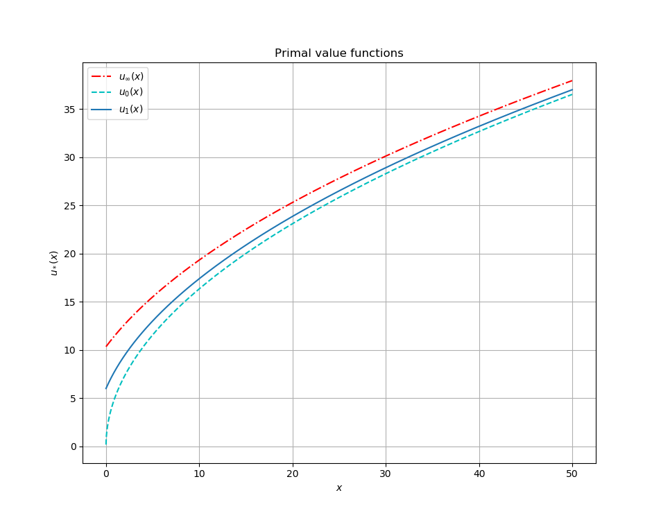
(a) Pre-income termination value function.

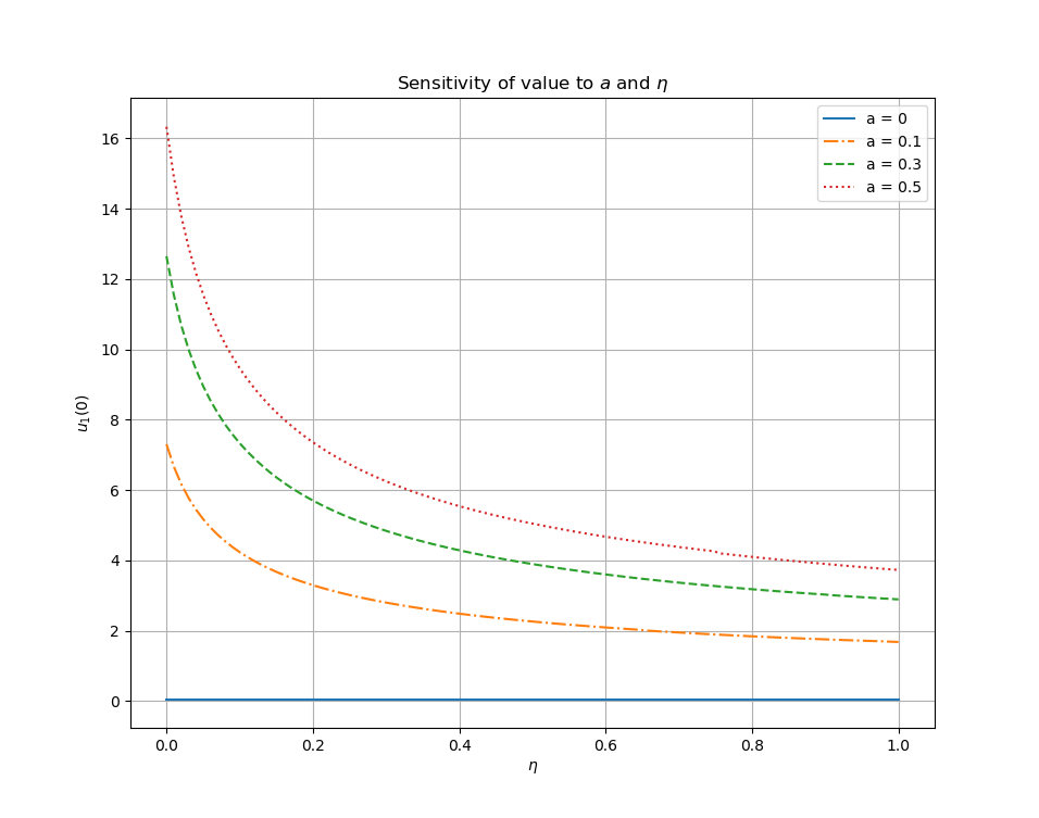
(b) Sensitivity of value function to $a$ and $\eta$.

Figure 1. Pre-income termination value function and the no-income and perpetual income value functions, and sensitivity of the value function to the income rate $a$ and termination intensity $\eta$ at zero wealth.

Figure 1 shows the value function $u_{1}(\cdot)$ as well as its bounding functions $u_{0}(\cdot)$ and $u_{\infty}(\cdot)$, also the dependence of the value function on the income rate $a$ and termination intensity $\eta$ at zero wealth. The data used are $\lambda=1$, $\sigma=0.1$, $\delta=0.6$, $\eta=0.1$, $a=0.2$, $p=0.5$.

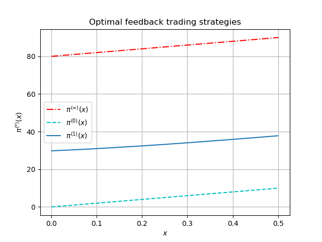
(a) Optimal feedback investment.

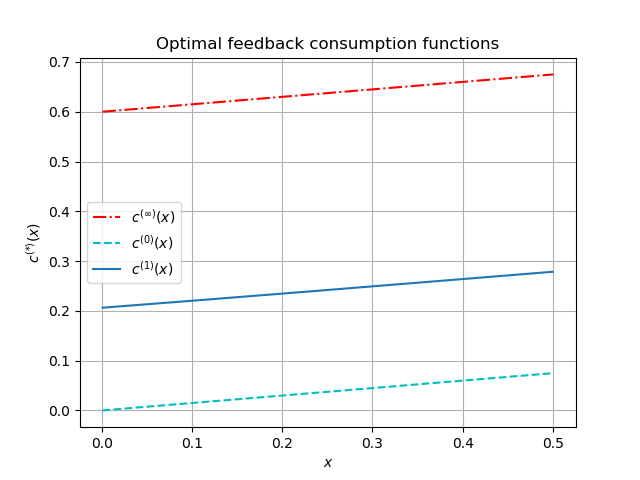
(b) Optimal feedback consumption.

Figure 2. Optimal feedback control functions associated with the pre-income termination value function $u_{1}(\cdot)$, and the no-income and perpetual income value functions $u_{0}(\cdot)$ and $u_{\infty}(\cdot)$.

Figure 2 shows the feedback control functions (for a smaller range near $x=0$ than in Figure 1). We can see the finite marginal utility at zero wealth of the pre-income termination value function and its explicit dependence on the income stream. We also note that both the optimal feedback controls are linear in wealth, as expected from (6.6) and (6.7).

7. Conclusions

In this paper we have proven a rigorous duality for an infinite horizon consumption problem with randomly terminating income, thereby closing the duality gap that arose in Vellekoop and Davis (2009), in a Black-Scholes market. The key property of the finiteness of marginal utility at zero initial wealth emerged, while all the other main tenets of duality theory were shown to hold. Our results readily extend to finite horizon versions of the problem as well.

There are still many aspects of such problems that are not well understood. One is to rigorously analyse the primal and dual HJB equations for the pre-income termination problem, for which the primal problem involves maximising utility from both consumption and inter-temporal wealth. The other is to fully understand the relations between the rather different forms of dual characterisation of utility maximisation problems with random endowment in the literature. We leave these questions for future research.

References

- Brannath and Schachermayer (1999) Brannath, W. and Schachermayer, W. (1999). A bipolar theorem for . In Séminaire de Probabilités, XXXIII, volume 1709 of Lecture Notes in Math., pages 349–354. Springer, Berlin.
- Cohen and Elliott (2015) Cohen, S. N. and Elliott, R. J. (2015). Stochastic calculus and applications. Probability and its Applications. Springer, Cham, second edition.
- Cvitanić et al. (2001) Cvitanić, J., Schachermayer, W., and Wang, H. (2001). Utility maximization in incomplete markets with random endowment. Finance Stoch., 5(2):259–272.
- Cvitanić et al. (2017) Cvitanić, J., Schachermayer, W., and Wang, H. (2017). Erratum to: Utility maximization in incomplete markets with random endowment [ MR1841719]. Finance Stoch., 21(3):867–872.