Magnetic field in relativistic heavy ion collisions: testing the classical approximation

Abstract

It is believed that in non-central relativistic heavy ion collisions a very strong magnetic field is formed. There are several studies of the effects of this field, where $\vec{B}$ is calculated with the expressions of classical electrodynamics. A quantum field may be approximated by a classical one when the number of field quanta in each field mode is sufficiently high. This may happen if the field sources are intense enough. In heavy ion physics the validity of the classical treatment was not investigated. In this work we propose a test of the quality of the classical approximation. We calculate an observable quantity using the classical magnetic field and also using photons as input. If the results of both approaches coincide, this will be an indication that the classical approximation is valid. More precisely, we focus on the process in which a nucleon is converted into a delta resonance, which then decays into another nucleon and a pion, i.e., $N\to\Delta\to N^{\prime}\pi$. In ultra-peripheral relativistic heavy ion collisions this conversion can be induced by the classical magnetic field of one the ions acting on the other ion. Alternatively, we can replace the classical magnetic field by a flux of equivalent photons, which are absorbed by the target nucleons. We calculate the cross sections in these two independent ways and find that they differ from each other by $\simeq 10$ % in the considered collision energy range. This suggests that the two formalisms are equivalent and that the classical approximation for the magnetic field is reasonable.

I Introduction

It has been often said that in relativistic heavy ion collisions we produce the strongest magnetic field of the universe skokov ; voro ; muller2 . This field is so intense because the charge density is large, because the speed of the source is very close to the speed of light and also because we probe it at extremely small distances (a few fermi) from the source.

There has been a search for observable effects of this strong field hattori . The first and most famous is the Chiral Magnetic Effect (CME) cme . A natural place to look for this field and its effects is in ultra-peripheral relativistic heavy ion collisions (UPC’s), in which the two nuclei do not overlap upc . Since there is no superposition of hadronic matter, the strong interaction is suppressed and the collision becomes essentially a very clean electromagnetic process.

In nos20 it was argued that forward pions are very likely to be produced by magnetic excitation (ME) of the nucleons in the nuclei. The strong classical magnetic field produced by one nucleus induces magnetic transitions, such as $N\to\Delta$ (where $N$ is a proton or a neutron), in the nucleons of the other nucleus. The produced $\Delta$ keeps moving together with the nucleus (or very close to it) and then decays almost exclusively through the reaction $\Delta\to N+\pi$. From the kinematics we know that the pion has a very large longitudinal momentum and very large rapidity. Since there is no other competing mechanism for forward pion production in UPC’s the observation of these pions would be a signature of the magnetic excitation of the nucleons and also an indirect measurement of the magnetic field. In nos20 it was shown that ME has a very large cross section.

The hypothesis that in heavy ion collisions the electromagnetic field can be treated classically and one can speak of a classical magnetic field has never been tested. The classical field approximation may be expected to become a reliable description of the quantum theory if the number of field quanta in each field mode is sufficiently high. In this work we propose a way to test the classical approximation for the magnetic field. To this end we consider again the process discussed in nos20

$$\hskip 184.9429ptN\,\to\,\Delta\,\to\,N^{\prime}\,\pi$$ (1)

but this time the transition is induced by photons and not by the classical magnetic field. We compute the same process using a different formalism where the quanta of the field play the important role. We then compare the results obtained with the two formalisms. In order to avoid uncertainties associated with the spatial distribution of the nuclear matter in the target we consider lead-proton collisions and choose to work in the proton rest-frame.

In the next section we briefly review the formalism used in nos20 which we shall call semi-classical and in the following section we describe the quantum formalism, based on the equivalent photon approximation. In the end we compare the results obtained with the two methods.

II The semi-classical formalism

A strong magnetic field can convert a hadron into another one with a different spin, by “flipping the constituent quark spins”. In ultra-relativistic heavy ion collisions this idea was first advanced in muller1 , where the authors studied the transition $\eta_{c}\to J/\psi$. In nos20 we extended the calculations to the $N\to\Delta$ transition.

Let us consider an ultra-peripheral $Pb-p$ collision, where the proton is at rest, as shown in Fig. 1. Under the influence of the strong magnetic field generated by the moving nucleus, the nucleon is converted into a $\Delta$. For the sake of definiteness let us consider the transition $|p\uparrow\rangle\to|\Delta^{+}\uparrow\rangle$. The amplitude for this process is given by nos20 ; muller1 :

$$a_{fi}=-i\int_{-\infty}^{\infty}e^{iE_{fi}t^{\prime}}\langle\Delta^{+}\uparrow|H_{int}(t^{\prime})|p\uparrow\rangle\,dt^{\prime}$$ (2)

where $\hbar=1$ and $E_{fi}=(m_{\Delta}^{2}-m_{n}^{2})/2m_{n}$, where $m_{\Delta}$ and $m_{n}$ are the $\Delta$ and nucleon masses respectively. The interaction Hamiltonian is given by:

$$H_{int}(t)=-\vec{\mu}.\vec{B}(t)$$ (3)

The magnetic dipole moment of the nucleon is given by the sum of the magnetic dipole moments of the corresponding constituent quarks:

$$\vec{\mu}=\sum_{i=u,d}\vec{\mu}_{i}=\sum_{i=u,d}\frac{q_{i}}{m_{i}}\vec{S}_{i}$$ (4)

where $q_{i}$ and $m_{i}$ are the charge and constituent mass of the quark of type $i$ and $\vec{S}_{i}$ is the spin operator acting on the spin state of this quark.

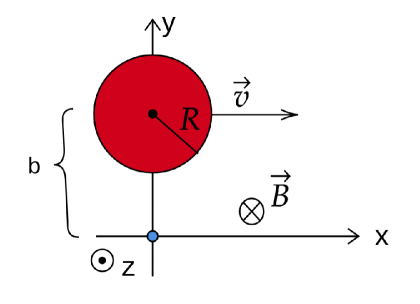
Figure 1: $Pb-p$ collision in the proton rest-frame. Coordinate system with magnetic field along the z direction. The projectile nucleus of radius $R$ moves with velocity $\vec{v}$ and impact parameter $b$. The blue circle represents the proton at rest.

In Fig. 1 we show the system of coordinates and the moving projectile. The projectile of radius $R$ moves along the x direction with impact parameter $b$ and the magnetic field is in the z direction. Since we are studying an UPC, we will, for simplicity, assume that the projectile-generated field is the same produced by a point charge. The field is given by muller2 :

$$B_{z}(t)=\frac{1}{4\pi}\frac{qv\gamma(b-y)}{((\gamma(x-vt))^{2}+(y-b)^{2}+z^{2})^{3/2}}$$ (5)

In the above expression $\gamma$ is the Lorentz factor, $b$ is the impact parameter along the $y$ direction, $v\simeq 1$ is the projectile velocity and the projectile electric charge is $q=Ze$.

The interaction Hamiltonian acts on spin states. The relevant ones are:

$$|p\uparrow\rangle=\frac{1}{3\sqrt{2}}[udu(\downarrow\uparrow\uparrow+\uparrow\uparrow\downarrow-2\uparrow\downarrow\uparrow)+duu(\uparrow\downarrow\uparrow+\uparrow\uparrow\downarrow-2\downarrow\uparrow\uparrow)+uud(\uparrow\downarrow\uparrow+\downarrow\uparrow\uparrow-2\uparrow\uparrow\downarrow)]$$ (6)

$$|\Delta^{+}\uparrow\rangle=\frac{1}{3}(uud+udu+duu)(\uparrow\uparrow\downarrow+\uparrow\downarrow\uparrow+\downarrow\uparrow\uparrow)$$ (7)

With these ingredients we can compute the matrix element $\langle\Delta^{+}\uparrow|H_{int}|p\uparrow\rangle$. It can be obtained by substituting Eqs. (4) and (5) into Eq. (3) and then calculating the sandwiches of $H_{int}$ with the spin states given above. Evaluating the nucleon-delta transition matrix element we find:

$$\langle\Delta^{+}\uparrow|H_{int}|p\uparrow\rangle\,=\,\frac{\sqrt{2}e}{3m}B_{z}$$ (8)

The cross section for a single $N\to\Delta$ transition is given by:

$$\sigma=\int|a_{fi}|^{2}\,d^{2}b=2\pi\,\int|a_{fi}|^{2}\,b\,db$$ (9)

where we have used cylindrical symmetry $d^{2}b\,=\,b\,db\,d\theta\to 2\,\pi\,b\,db$. Inserting (8) into (2) and using it in the above expression we find:

$$\sigma=\frac{Z^{2}e^{4}}{9\pi m^{2}}\left(\frac{E_{fi}}{v\gamma}\right)^{2}\int_{R}^{\infty}\Big{[}K_{1}\Big{(}\frac{E_{fi}b}{v\gamma}\Big{)}\Big{]}^{2}b\,db$$ (10)

where $K_{1}$ is the modified Bessel function. This is the result obtained with the semi-classical approach. For the purpose of this work it is enough to consider a nucleon as a target. In nos20 we computed the cross section for a nucleus-nucleus collision.

III The quantum formalism

In the quantum formalism, the electromagnetic field produced by an ultra-relativistic electric charge is replaced by a flux of photons upc .

Figure 2: Quantum version of the process depicted in Fig. 1. Pion photoproduction through a $\Delta$ resonance.

Now, in a high energy UPC, the projectile becomes a source of almost real photons and we replace the classical field by a collection of quanta. Thus, the cross section of the process (1) can be written in a factorized form in terms of the photon flux produced by the projectile and the photon-nucleon cross section upc :

$$\sigma=\int\frac{d\omega}{\omega}\,n(\omega)\,\sigma_{\gamma N\rightarrow N\pi}(\omega)$$ (11)

In the above expression $n(\omega)$ represents the photon spectrum generated by the source upc :

$$n(\omega)=\frac{Z^{2}\alpha}{\pi}\Bigg{[}2\xi K_{0}(\xi)K_{1}(\xi)-\xi^{2}[K_{1}^{2}(\xi)-K_{0}^{2}(\xi)]\Bigg{]},\hskip 56.9055pt\xi=\frac{\omega(R_{1}+R_{2})}{\gamma}$$ (12)

where $\omega$ is the photon energy, $R_{1}$ and $R_{2}$ are the radii of the projectile and the target, parametrized as $R_{A}=1.2\,A^{1/3}fm$, and $\gamma$ the Lorentz boost in the target frame. From the above expression it is clear that the average energy carried by an emitted photon increases with $\gamma$ and hence with the collision energy $\sqrt{s}$. The photon average energy may be estimated as

$$\bar{\omega}=\frac{\int_{0}^{\gamma m_{n}}\,n(\omega)\,\omega\,d\omega}{\int_{0}^{\gamma m_{n}}\,n(\omega)\,d\omega}$$ (13)

In the LHC energy region $\gamma\simeq 1000$ and the above expression yields $\bar{\omega}\simeq 10$ GeV.

In order to perform the calculation of the total cross section, it is necessary to know the cross section of the process $\gamma N\rightarrow N\pi$. In a first approximation $\sigma_{\gamma N\rightarrow N\pi}$ can be calculated evaluating the Feynman diagram shown in Fig. 2. This is a very well known process. In fact, there is an intense effort devoted to the study of nucleon resonances both experimentally and theoretically ire20 ; pasca ; clas ; ab ; manolo20 ; gil19 . Most of the interest lies on the energy region around the threshold of $\Delta$ production, i.e., $\bar{\omega}\simeq 200-600$ MeV. As it was just mentioned above, we are primarily interested in the high energy region, far from this threshold. We need a formula which correctly reproduces the behavior of the cross section in the $\Delta$ resonance region and which can be extrapolated to higher energies. This is the most important source of uncertainty in the evaluation of (11).

A simple parametrization of the $\pi^{0}$ photoproduction cross section can be taken from Jones and Scadron Jones :

$$\sigma_{\gamma N\rightarrow N\pi}(\omega)=2\pi\int_{0}^{\pi}d\theta\,\sin{\theta}\,\frac{\alpha\,\omega}{12\,m_{n}\,W}\,\frac{\sin^{2}\delta}{\Gamma}\,\left[\,|F_{+}^{*}|^{2}\,f(\theta)\,+\,|G_{+}^{*}|^{2}\,g(\theta)\,\right]$$ (14)

In the above expression $\alpha=1/137$, $W^{2}=m_{n}^{2}+2\,\omega\,m_{n}$ is the photon-nucleon center of mass energy squared, $m_{n}$ is the nucleon mass, $\Gamma$ is the $\Delta$ decay width and $F_{+}^{*}=G_{M}^{*}-3G_{E}^{*}$, $G_{+}^{*}=G_{M}^{*}+G_{E}^{*}$. The form factors $G_{M}^{*}$ and $G_{E}^{*}$ are functions of the photon virtuality $Q^{2}$. Since we are interested in photoproduction they are taken at $Q^{2}=0$. The calculations were all carried out in the laboratory frame. The angular dependence is given by $f(\theta)=(3\cos^{2}\theta+1)/2$, $g(\theta)=(9\sin^{2}\theta)/2$ and

$$\sin^{2}\delta=|\frac{m_{\Delta}\Gamma}{(W^{2}-m_{\Delta}^{2}+im_{\Delta}\Gamma})|^{2}$$ (15)

The expression (14) contains three parameters $G_{M}^{*}$, $G_{E}^{*}$ and $\Gamma$, which can be determined by fitting the experimental data on $\pi^{0}$ photoproduction. We have adjusted (14) to the data published in datadel . The result is shown in Fig. 3. In order to estimate the uncertainty in the extrapolation of (14) to higher photon energies we have varied the $\Delta$ width within the interval $100<\Gamma<120$ MeV. As it can be seen, the high energy tail of the curve is not very sensitive to changes in $\Gamma$. The uncertainties in $G_{M}^{*}(0)$ and $G_{E}^{*}(0)$ are very small and changes of these quantities would not significantly change the cross sections.

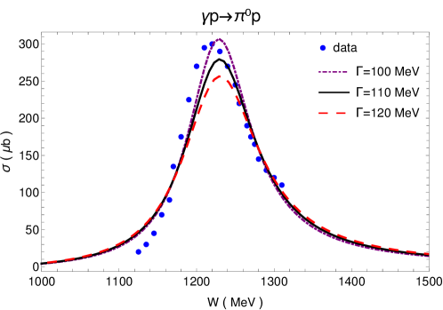
Figure 3: Pion photoproduction. Comparison between the theory, Eq. (14), and data from datadel .

Having determined $\sigma_{\gamma N\rightarrow N\pi}$, we insert it into (11) and evaluate the cross section of the quantum process. The results are then compared with the results obtained with the semi-classical approach (given by (10)) and presented in Fig. 4. The cross sections are plotted as a function of the energy per nucleon (of the projectile) in the laboratory frame $E_{Lab}=\gamma\,m_{n}$. In the upper pannel we compare the curves obtained with (10) (dashed line) and with (11) (solid lines). The band in the lower curve represents the different choices of the width $\Gamma$, i.e., the different values shown in Fig. 3. In the lower pannel we show (10) divided by the central value of (11). This ratio quantifies the difference between these two curves and it approaches 9 % at the highest energies.

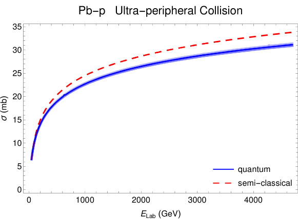
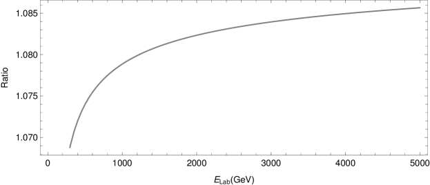
Figure 4: Comparison between the semi-classical and quantum cross sections of pion photoproduction in an ultra-peripheral lead-nucleon collision. Upper pannel: cross sections as a function of the energy per nucleon in the laboratory frame. Lower pannel: ratio between semi-classical and quantum cross sections.

These results suggest that the classical approximation of the magnetic field reproduces most of the photon interaction in photoproduction in high energies.

The quantum formula (14) could be improved. At low energies there are other resonances. To improve the accuracy of the extrapolation to higher photon energies, it would be necessary to change (14) including higher resonances or, alternatively, define some procedure to “average over the bumps”, as it was done (although in a different context), for example, in brona .

IV Concluding remarks

In heavy ion collisions the sources are so intense that one can treat classically the electromagnetic field. In particular, one can compute the magnetic field and use it to make a number of predictions. Although plausible, this conjecture had never been tested before. In this work we have devised a test for this idea. We have found a process which can be calculated in two different ways: one using the magnetic field and one relying solely on quantum physics. The EPA method has been extensively used and has yielded predictions confirmed by experimental data.

Our results give some support to the classical approximation for the magnetic field and hence give support to all the calculations done previously based on this approximation.

- (1) V. Skokov, A. Y. Illarionov and V. Toneev, Int. J. Mod. Phys. A 24, 5925 (2009).
- (2) V. Voronyuk, V. D. Toneev, W. Cassing, E. L. Bratkovskaya, V. P. Konchakovski and S. A. Voloshin, Phys. Rev. C 83, 054911 (2011).
- (3) M. Asakawa, A. Majumder and B. Muller, Phys. Rev. C 81, 064912 (2010).
- (4) For a recent review see K. Hattori and X. G. Huang, Nucl. Sci. Tech. 28, 26 (2017) and references therein; A. Dubla, U. Gürsoy and R. Snellings, arXiv:2009.09727; C. S. Machado, F. S. Navarra, E. G. de Oliveira, J. Noronha and M. Strickland, Phys. Rev. D 88, 034009 (2013).
- (5) K. Fukushima, D. E. Kharzeev and H. J. Warringa, Phys. Rev. D 78, 074033 (2008).
- (6) C. A. Bertulani, S. R. Klein and J. Nystrand, Ann. Rev. Nucl. Part. Sci. 55, 271 (2005); V. P. Goncalves and M. V. T. Machado, Eur. Phys. J. C 40, 519 (2005).
- (7) I. Danhoni and F. S. Navarra, Phys. Lett. B 805, 135463 (2020).
- (8) D. L. Yang and B. Muller, J. Phys. G 39, 015007 (2012).
- (9) For a very recent and comprehensive theoretical and experimental review, see D. G. Ireland, E. Pasyuk and I. Strakovsky, Prog. Part. Nucl. Phys. 111, 103752 (2020) and references therein.
- (10) V. Pascalutsa, M. Vanderhaeghen and S. N. Yang, Phys. Rept. 437, 125 (2007).
- (11) I. G. Aznauryan et al. [CLAS Collaboration], Phys. Rev. C 80, 055203 (2009).
- (12) I. G. Aznauryan and V. D. Burkert, Prog. Part. Nucl. Phys. 67, 1 (2012).
- (13) G. H. G. Navarro and M. J. Vicente Vacas, arXiv:2008.04244 [hep-ph].
- (14) G. Ramalho, Phys. Rev. D 100, 114014 (2019); Eur. Phys. J. A 55, 32 (2019); Eur. Phys. J. A 54, 75 (2018); Phys. Rev. D 94, 114001 (2016).
- (15) H.F. Jones and M.D. Scadron, Annals of Phys. 81, 1 (1973).
- (16) D. A. McPherson, D. C. Gates, R. W. Kenney and W. P. Swanson, Phys. Rev. 136, B1465 (1964); M. MacCormick et al., Phys. Rev. C 53, 41 (1996).
- (17) S. J. Brodsky and F. S. Navarra, Phys. Lett. B 411, 152 (1997).