Noise-Contrastive Estimation for Multivariate Point Processes

Abstract

The log-likelihood of a generative model often involves both positive and negative terms. For a temporal multivariate point process, the negative term sums over all the possible event types at each time and also integrates over all the possible times. As a result, maximum likelihood estimation is expensive. We show how to instead apply a version of noise-contrastive estimation—a general parameter estimation method with a less expensive stochastic objective. Our specific instantiation of this general idea works out in an interestingly non-trivial way and has provable guarantees for its optimality, consistency and efficiency. On several synthetic and real-world datasets, our method shows benefits: for the model to achieve the same level of log-likelihood on held-out data, our method needs considerably fewer function evaluations and less wall-clock time.

1 Introduction

Maximum likelihood estimation (MLE) is a popular training method for generative models. However, to obtain the likelihood of a generative model given the observed data, one must compute the probability of each observed sample, which often includes an expensive normalizing constant. For example, in a language model, each word is typically drawn from a softmax distribution over a large vocabulary, whose normalizing constant requires a summation over the vocabulary.

This paper aims to alleviate a similar computational cost for multivariate point processes. These generative models are natural tools to analyze streams of discrete events in continuous time. Their likelihood is improved not only by raising the probability of the observed events, but by lowering the probabilities of the events that were observed not to occur. There are infinitely many times at which no event of any type occurred; to predict these non-occurrences, the likelihood must integrate the infinitesimal event probability for each event type over the entire observed time interval. Therefore, the likelihood is expensive to compute, particularly when there are many possible event types.

As an alternative to MLE, we propose to train the model by learning to discriminate the observed events from events sampled from a noise process. Our method is a version of noise-contrastive estimation (NCE), which was originally developed for unnormalized (energy-based) distributions and then extended to conditional softmax distributions such as language models. To our best knowledge, we are the first to extend the method and its theoretical guarantees (for optimality, consistency and efficiency) to the context of multivariate point processes. We will also discuss similar efforts in related areas in section 4.

On several datasets, our method shows compelling results. By evaluating fewer event intensities, training takes much less wall-clock time while still achieving competitive log-likelihood.

2 Preliminaries

2.1 Event Streams and Multivariate Point Processes

Given a fixed time interval $[0,T)$, we may observe an event stream $x_{[0,T)}$: at each continuous time $t$, the observation $x_{t}$ is one of the discrete types $\{\varnothing,1,\ldots,K\}$ where $\varnothing$ means no event. An non-$\varnothing$ observation is called an event. A generative model of an event stream is called a multivariate point process.

We wish to fit an autoregressive probability model to observed event streams. In a discrete-time autoregressive model, events would be generated from left to right, where $x_{t}$ is drawn from a distribution that depends on $x_{0},\ldots,x_{t-1}$. The continuous-time version still generates events from left to right, but at any specific time $t$ we have $p(x_{t}=\varnothing)=1$, with only an infinitesimal probability of any event. (For a computationally practical sampling method, see section 3.1.) The model is a stochastic process defined by functions $\lambda_{k}$ that determine a finite intensity $\lambda_{{k}}(t\mid x_{[0,t)})\geq 0$ for each event type $k\neq\varnothing$ at each time $t>0$. This intensity depends on the history of events $x_{[0,t)}$ that were drawn at times $<t$. It quantifies the instantaneous rate at time $t$ of events of type $k$. That is, $\lambda_{{k}}(t\mid x_{[0,t)})$ is the limit as $dt\rightarrow^{+}0$ of $\tfrac{1}{dt}$ times the expected number of events of type $k$ on the interval $[t,t+dt)$, where the expectation is conditioned on the history.

As the event probabilities are infinitesimal, the times of the events are almost surely distinct. To ensure that we have a point process, the intensity functions must be chosen such that the total number of events on any bounded interval is almost surely finite. Models of this form include inhomogeneous Poisson processes (Daley & Vere-Jones, 2007), in which the intensity functions ignore the history, as well as (non-explosive) Hawkes processes (Hawkes, 1971) and their modern neural versions (Du et al., 2016; Mei & Eisner, 2017).

Most models use intensity functions that are continuous between events. Our analysis requires only

Assumption 1 (Continuity).

For any event stream $x_{[0,T)}$ and event type $k\in\{1,\ldots,K\}$, $\lambda_{{k}}(t\mid x_{[0,t)})$ is Riemann integrable, i.e., bounded and continuous almost everywhere w.r.t. time $t$.

2.2 Maximum Likelihood Estimation: Usefulness and Difficulties

In practice, we parameterize the intensity functions by $\theta$. We write $p_{\theta}$ for the resulting probability density over event streams. When learning $\theta$ from data, we make the conventional assumption that the true point process $p^{*}$ actually falls into the chosen model family:

Assumption 2 (Existence).

There exists at least one parameter vector $\theta^{*}$ such that $p_{\theta^{*}}=p^{*}$.

Then as proved in Appendix A, such a $\theta^{*}$ can be found as an argmax of

$$J_{\mathrm{LL}}(\theta)\mathrel{\stackrel{{\scriptstyle\textnormal{\tiny def}}}{{=}}}\mathbb{E}_{{x_{[0,T)}\sim p^{*}}}\left[\log p_{\theta}(x_{[0,T)})\right]$$ (1)

Given assumption 1, the $\theta$ values that maximize $J_{\mathrm{LL}}(\theta)$ are exactly the set $\Theta^{*}$ of values for which $p_{\theta}=p^{*}$: any $\theta$ for which $p_{\theta}\neq p^{*}$ would end up with a strictly smaller $J_{\mathrm{LL}}(\theta)$ by increasing the cross entropy $-p^{*}\log p_{\theta}$ over some interval $(t,t^{\prime})$ for a set of histories with non-zero measure.

If we modify equation 1 to take the expectation under the empirical distribution of event streams $x_{[0,T)}$ in the training dataset, then $J_{\mathrm{LL}}(\theta)$ is proportional to the log-likelihood of $\theta$. For any $x_{[0,T)}$ that satisfies the condition in assumption 1, the log-density used in equation 1 can be expressed in terms of $\lambda_{{k}}(t\mid x_{[0,t)})$:

$$\log p_{\theta}(x_{[0,T)})=\sum_{t:x_{t}\neq\varnothing}\log\lambda_{{x_{t}}}(t\mid x_{[0,t)})-\int_{t=0}^{T}\sum_{k=1}^{K}\lambda_{{k}}(t\mid x_{[0,t)})dt$$ (2)

Notice that the second term lacks a log. It is expensive to compute in the following cases:

• The total number of event types $K$ is large, making $\sum_{k=1}^{K}$ slow.

• The integral $\int_{t=0}^{T}$ is slow to estimate well, e.g., via a Monte Carlo estimate $\tfrac{T}{J}\sum_{j=1}^{J}\sum_{k=1}^{K}\lambda_{{k}}(t_{j})$ where each $t_{j}$ is randomly sampled from the uniform distribution over $[0,T)$.

• The chosen model architecture makes it hard to parallelize the $\lambda_{{k}}(t_{j})$ computation over $j$ and $k$.

2.3 Noise-Contrastive Estimation in Discrete Time

For autoregressive models of discrete-time sequences, a similar computational inefficiency can be tackled by applying the principle of noise-contrastive estimation (Gutmann & Hyvärinen, 2010), as follows. For each history $x_{0:t}\mathrel{\stackrel{{\scriptstyle\textnormal{\tiny def}}}{{=}}}x_{0}x_{1}\ldots x_{t-1}$ in training data, NCE trains the model $p_{\theta}$ to discriminate the actually observed datum $x_{t}$ from some noise samples whose distribution $q$ is known. The intuition is: optimal performance is obtained if and only if $p_{\theta}$ matches the true distribution $p^{*}$.

More precisely, given a bag $\{x_{t}^{0},x_{t}^{1},\ldots,x_{t}^{M}\}$, where exactly one element of the bag was drawn from $p^{*}$ and the rest drawn i.i.d. from $q$, consider the log-posterior probability (via Bayes’ Theorem) that $x_{t}^{0}$ was the one drawn from $p^{*}$:

$$\hskip 56.9055pt\log\tfrac{\phantom{\sum_{m=0}^{M}}p^{*}(x_{t}^{0}\mid x_{0:t})\prod_{m=1}^{M}q(x_{t}^{m}\mid x_{0:t})}{\sum_{m=0}^{M}p^{*}(x_{t}^{m}\mid x_{0:t})\prod_{m^{\prime}\neq m}q(x_{t}^{m^{\prime}}\mid x_{0:t})}$$ (3)

The “ranking” variant of NCE (Jozefowicz et al., 2016) substitutes $p_{\theta}$ for $p^{*}$ in this expression, and seeks $\theta$ (e.g., by stochastic gradient ascent) to maximize the expectation of the resulting quantity when $x_{t}^{0}$ is a random observation in training data, $x_{0:t}$ is its history, and $x_{t}^{1},\ldots,x_{t}^{M}$ are drawn i.i.d. from $q(\cdot\mid x_{0:t})$.

This objective is really just conditional maximum log-likelihood on a supervised dataset of $(M+1)$-way classification problems. Each problem presents an unordered set of $M+1$ samples—one drawn from $p^{*}$ and the others drawn i.i.d. from $q$. The task is to guess which sample was drawn from $p^{*}$. Conditional MLE trains $\theta$ to maximize (in expectation) the log-probability that the model assigns to the correct answer. In the infinite-data limit, it will find $\theta$ (if possible) such that these log-probabilities match the true ones given by (3). For that, it is sufficient for $\theta$ to be such that $p_{\theta}=p^{*}$. Given assumption 2, Ma & Collins (2018) show that $p_{\theta}=p^{*}$ is also necessary, i.e., the NCE task is sufficient to find the true parameters. Although the NCE objective does not learn to predict the full observed sample $x_{t}$ as MLE does, but only to distinguish it from the $M$ noise samples, their theorem implies that in expectation over all possible sets of $M$ noise samples, it actually retains all the information (provided that $M>0$ and $q$ has support everywhere that $p^{*}$ does).

This NCE objective is computationally cheaper than MLE when the distribution $p_{\theta}(\cdot\mid x_{0:t})$ is a softmax distribution over $\{1,\ldots,K\}$ with large $K$. The reason is that the expensive normalizing constants in the numerator and denominator of equation 3 need not be computed. They cancel out because all the probabilities are conditioned on the same (actually observed) history.

3 Applying Noise-Contrastive Estimation in Continuous Time

The expensive $\int\sum$ term in equation 2 is rather similar to a normalizing constant, as it sums over non-occurring events. We might try to avoid computing it by discretizing the time interval $[0,T)$ into finitely many intervals of width $\Delta$ and applying NCE. In this case, we would be distinguishing the true sequence of events on an interval $[i\Delta,(i+1)\Delta)$ from corresponding noise sequences on the same interval, given the same (actually observed) history $x_{[0,i\Delta)}$. Unfortunately, the distribution $p_{\theta}(\cdot\mid x_{[0,i\Delta)})$ in the objective still involves an $\int\sum$ term where the integral is over $[i\Delta,(i+1)\Delta)$ and the inner sum is over $k$. The solution is to shrink the intervals to infinitesimal width $dt$. Then our log-posterior over each of them becomes

$$\log\dfrac{\phantom{\sum_{m=0}^{M}}{p}_{\theta}(x_{[t,t+dt)}^{0}\mid x_{[0,t)}^{0})\prod_{m=1}^{M}q(x_{[t,t+dt)}^{0}\mid x_{[0,t)}^{0})}{\sum_{m=0}^{M}{p}_{\theta}(x_{[t,t+dt)}^{m}\mid x_{[0,t)}^{0})\prod_{m^{\prime}\neq m}q(x_{[t,t+dt)}^{m^{\prime}}\mid x_{[0,t)}^{0})}$$ (4)

We will define the noise distribution $q$ in terms of finite intensity functions $\lambda^{\mathrm{q}}_{{k}}$, like the ones $\lambda_{{k}}$ that define $p_{\theta}$. As a result, at a given time $t$, there is only an infinitesimal probability that any of $\{x_{t}^{0},x_{t}^{1},\ldots,x_{t}^{M}\}$ is an event. Nonetheless, at each time $t\in[0,T)$, we will consider generating a noise event (for each $m>0$) conditioned on the actually observed history $x_{[0,t)}$. Among these uncountably many times $t$, we may have some for which $x_{t}^{0}\neq\varnothing$ (the observed events), or where $x_{t}^{m}\neq\varnothing$ for some $1\leq m\leq M$ (the noise events).

Almost surely, the set of times $t$ with a real or noise event remains finite. Our NCE objective is the expected sum of equation 4 over all such times $t$ in an event stream, when the stream is drawn uniformly from the set of streams in the training dataset—as in 3—and the noise events are then drawn as above.

Our objective ignores all other times $t$, as they provide no information about $\theta$. After all, when $x_{t}^{0}=\cdots=x_{t}^{M}=\varnothing$, the probability that $x_{t}^{0}$ is the one drawn from the true model must be $1/(M+1)$ by symmetry, regardless of $\theta$. At these times, the ratio in equation 4 does reduce to $1/(M+1)$, since all probabilities are 1.

At the times $t$ that we do consider, how do we compute equation 4? Almost surely, exactly one of $x_{t}^{0},\ldots,x_{t}^{M}$ is an event $k$ for some $k\neq\varnothing$. As a result, exactly one factor in each product is infinitesimal ($dt$ times the $\lambda_{{k}}$ or $\lambda^{\mathrm{q}}_{{k}}$ intensity), and the other factors are 1. Thus, the $dt$ factors cancel out between numerator and denominator, and equation 4 simplifies to

$$\log\tfrac{\lambda_{{k}}(t\mid x_{[0,t)}^{0})}{\lambda_{{k}}(t\mid x_{[0,t)}^{0})+M\lambda^{\mathrm{q}}_{{k}}(t\mid x_{[0,t)}^{0})}\text{ if }x_{t}^{0}=k\text{ and }\log\tfrac{\lambda^{\mathrm{q}}_{{k}}(t\mid x_{[0,t)}^{0})}{\lambda_{{k}}(t\mid x_{[0,t)}^{0})+M\lambda^{\mathrm{q}}_{{k}}(t\mid x_{[0,t)}^{0})}\text{ if }x_{t}^{0}=\varnothing$$ (5)

When a gradient-based optimization method adjusts $\theta$ to increase equation 5, the intuition is as follows. If $x_{t}^{0}=k$, the model intensity $\lambda_{{k}}(t)$ is increased to explain why an event of type $k$ occurred at this particular time $t$. If $x_{t}^{0}=\varnothing$, the model intensity $\lambda_{{k}}(t)$ is decreased to explain why an event of type $k$ did not actually occur at time $t$ (it was merely a noise event $x_{t}^{m}=k$, for some $m\neq 0$). These cases achieve the same qualitative effects as following the gradients of the first and second terms, respectively, in the log-likelihood (2).

Our full objective is an expectation of the sum of finitely many such log-ratios:

$$J_{\mathrm{NC}}(\theta)\mathrel{\stackrel{{\scriptstyle\textnormal{\tiny def}}}{{=}}}\mathbb{E}_{{x_{[0,T)}^{0}\sim p^{*},x_{[0,T)}^{1:M}\sim q}}\left[\sum_{t:x_{t}^{0}\neq\varnothing}\log\tfrac{\lambda_{{x_{t}^{0}}}(t\mid x_{[0,t)}^{0})}{\underline{\lambda}_{x_{t}^{0}}(t\mid x_{[0,t)}^{0})}+\sum_{m=1}^{M}\sum_{t:x_{t}^{m}\neq\varnothing}\log\tfrac{\lambda^{\mathrm{q}}_{{x_{t}^{m}}}(t\mid x_{[0,t)}^{0})}{\underline{\lambda}_{x_{t}^{m}}(t\mid x_{[0,t)}^{0})}\right]$$ (6)

where $\underline{\lambda}_{k}(t\mid x_{[0,t)}^{0})\mathrel{\stackrel{{\scriptstyle\textnormal{\tiny def}}}{{=}}}\lambda_{{k}}(t\mid x_{[0,t)}^{0})+M\lambda^{\mathrm{q}}_{{k}}(t\mid x_{[0,t)}^{0})$. The expectation is estimated by sampling: we draw an observed stream $x_{[0,T)}^{0}$ from the training dataset, then draw noise events $x_{[0,T)}^{1:M}$ from $q$ conditioned on the prefixes (histories) given by this observed stream, as explained in the next section. Given these samples, the bracketed term is easy to compute (and we then use backprop to get its gradient w.r.t. $\theta$, which is a stochastic gradient of the objective (6)). It eliminates the $\int\sum$ of equation 2 as desired, replacing it with a sum over the noise events. For each real or noise event, we compute only two intensities—the true and noise intensities of that event type at that time.

3.1 Efficient Sampling of Noise Events

The thinning algorithm (Lewis & Shedler, 1979; Liniger, 2009) is a rejection sampling method for drawing an event stream over a given observation interval $[0,T)$ from a continuous-time autoregressive process. Suppose we have already drawn the first $i-1$ times, namely $t_{1},\ldots,t_{i-1}$. For every future time $t\geq t_{i-1}$, let $\mathcal{H}(t)$ denote the context $x_{[0,t)}$ consisting only of the events at those times, and define $\lambda(t\mid\mathcal{H}(t))\mathrel{\stackrel{{\scriptstyle\textnormal{\tiny def}}}{{=}}}\sum_{k=1}^{K}\lambda_{{k}}(t\mid\mathcal{H}(t))$. If $\lambda(t\mid\mathcal{H}(t))$ were constant at $\overline{\lambda}$, we could draw the next event time as $t_{i}\sim t_{i-1}+\mathrm{Exp}(\overline{\lambda})$. We would then set $x_{t}=\varnothing$ for all of the intermediate times $t\in(t_{i-1},t_{i})$, and finally draw the type $x_{t_{i}}$ of the event at time $t_{i}$, choosing $k$ with probability $\lambda_{{k}}(t_{i}\mid\mathcal{H}(t))\,/\,\overline{\lambda}$. But what if $\lambda(t\mid\mathcal{H}(t))$ is not constant? The thinning algorithm still runs the foregoing method, taking $\overline{\lambda}$ to be any upper bound: $\overline{\lambda}\geq\lambda(t\mid\mathcal{H}(t))$ for all $t\geq t_{i-1}$. In this case, there may be “leftover” probability mass not allocated to any $k$. This mass is allocated to $\varnothing$. A draw of $x_{t_{i}}=\varnothing$ means there was no event at time $t_{i}$ after all (corresponding to a rejected proposal). Either way, we now continue on to draw $t_{i+1}$ and $x_{t_{i+1}}$, using a version of $\mathcal{H}(t)$ that has been updated to include the event or non-event $x_{t_{i}}$. The update to $\mathcal{H}(t)$ affects $\lambda(t\mid\mathcal{H}(t))$ and the choice of $\overline{\lambda}$.

How to sample noise streams. To draw a stream $x_{[0,t)}^{m}$ of noise events, we run the thinning algorithm, using the noise intensity functions $\lambda^{\mathrm{q}}_{{k}}$. However, there is a modification: $\mathcal{H}(t)$ is now defined to be $x_{[0,t)}^{0}$—the history from the observed event stream, rather than the previously sampled noise events—and is updated accordingly. This is because in equation 6, at each time $t$, all of $\{x_{t}^{0},x_{t}^{1},\ldots,x_{t}^{M}\}$ are conditioned on $x_{[0,t)}^{0}$ (akin to the discrete-time case). The full pseudocode is given in Algorithm 1 in the supplementary material.

Coarse-to-fine sampling of event types. Although our NCE method has eliminated the need to integrate over $t$, the thinning algorithm above still sums over $k$ in the definition of $\lambda^{\mathrm{q}}(t\mid\mathcal{H}(t))$. For large $K$, this sum is expensive if we take the noise distribution on each training minibatch to be, for example, the $p_{\theta}$ with the current value of $\theta$. That is a statistically efficient choice of noise distribution, but we can make a more computationally efficient choice. A simple scheme is to first generate each noise event with a coarse-grained type $c\in\{1,\ldots,C\}$, and then stochastically choose a refinement $k\in\{1,\ldots,K\}$:

$$\lambda^{\mathrm{q}}_{{k}}(t\mid x_{[0,t)}^{0}) \mathrel{\stackrel{{\scriptstyle\textnormal{\tiny def}}}{{=}}}\sum_{c=1}^{C}q(k\mid c)\lambda^{\mathrm{q}}_{{c}}(t\mid x_{[0,t)}^{0})\text{ for }k=1,2,\ldots,K$$ (7)

This noise model is parameterized by the functions $\lambda^{\mathrm{q}}_{{c}}$ and the probabilities $q(k\mid c)$. The total intensity is now $\lambda^{\mathrm{q}}(t\mid\mathcal{H}(t))=\sum_{c=1}^{C}\lambda^{\mathrm{q}}_{{c}}(t)$, so we now need to examine only $C$ intensity functions, not $K$, to choose $\overline{\lambda}$ in the thinning algorithm. If we partition the $K$ types into $C$ coarse-grained clusters (e.g., using domain knowledge), then evaluating the noise probability (7) within the training objective (6) is also fast because there is only one non-zero summand $c$ in equation 7. This simple scheme works well in our experiments. However, it could be elaborated by replacing $q(k\mid c)$ with $q(k\mid c,x_{[0,t)}^{0})$, by partitioning the event vocabulary automatically, by allowing overlapping clusters, or by using multiple levels of refinement: all of these elaborations are used by the fast hierarchical language model of Mnih & Hinton (2009).

How to draw $M$ streams. An efficient way to draw the union of $M$ i.i.d. noise streams is to run the thinning algorithm once, with all intensities multiplied by $M$. In other words, the expected number of noise events on any interval is multiplied by $M$. This scheme does not tell us which specific noise stream $m$ generated a particular noise event, but the NCE objective (6) does not need to know that. The scheme works only because every noise stream $m$ has the same intensities $\lambda^{\mathrm{q}}_{{k}}(t\mid x_{[0,t)}^{0})$ (not $\lambda^{\mathrm{q}}_{{k}}(t\mid x_{[0,t)}^{m})$) at time $t$: there is no dependence on the previous events from that stream. Amusingly, NCE can now run even with non-integer $M$.

Fractional objective. One view of the thinning algorithm is that it accepts the proposed time $t_{i}$ with probability $\mu=\lambda(t_{i})/\overline{\lambda}$, and in that case, labels it as $k$ with probability $\lambda_{{k}}(t_{i})/\lambda(t_{i})$. To get a greater diversity of noise samples, we can accept the time with probability 1, if we then scale its term in the objective (6) by $\mu$. This does not change the expectation (6) but may reduce the sampling variance in estimating it. Note that increasing the upper bound $\overline{\lambda}$ now has an effect similar to increasing $M$: more noise samples.

3.2 Computational Cost Analysis

State-of-the-art intensity models use neural networks whose state summarizes the history and is updated after each event. So to train on a single event stream $x$ with $I\geq 0$ events, both MLE and NCE must perform $I$ updates to the neural state. Both MLE and NCE then evaluate the intensities $\lambda_{{k}}(t\mid x_{[0,t)})$ of these $I$ events, and also the intensities of a number of events that did not occur, which almost surely fall at other times.

Consider the number of intensities evaluated. For MLE, assume the Monte Carlo integration technique mentioned in section 2.2. MLE computes the intensity $\lambda$ for $I$ observed events and for all $K$ possible events at each of $J$ sampled times. We take $J=\rho I$ (with randomized rounding to an integer), where $\rho>0$ is a hyperparameter (Mei & Eisner, 2017). Hence, the expected total number of intensity evaluations is $I+\rho IK$.

For NCE with the coarse-to-fine strategy, let $J$ be the total number of times proposed by the thinning algorithm. Observe that $\mathbb{E}\left[I\right]=\int_{0}^{T}\lambda^{*}(t\mid x_{[0,t)})dt$, and $\mathbb{E}\left[J\right]=M\cdot\int_{0}^{T}\overline{\lambda}(t\mid x_{[0,t)})dt$. Thus, $\mathbb{E}\left[J\right]\approx M\cdot\mathbb{E}\left[I\right]$ if (1) $\overline{\lambda}$ at any time is a tight upper bound on the noise event rate $\lambda^{\mathrm{q}}$ at that time and (2) the average noise event rate well-approximates the average observed event rate (which should become true very early in training). To label or reject each of the $J$ proposals, NCE evaluates $C$ noise intensities $\lambda^{\mathrm{q}}_{{c}}$; if the proposal is accepted with label $k$ (perhaps fractionally), it must also evaluate its model intensity $\lambda_{{k}}$. The noise and model intensities $\lambda^{\mathrm{q}}_{{c}}$ and $\lambda_{{k}}$ must also be evaluated for the $I$ observed events. Hence, the total number of intensity evaluations is at most $(C+1)J+2I$, which $\approx(C+1)MI+2I$ in expectation.

Dividing by $I$, we see that making $(M+1)(C+1)\leq\rho K$ suffices to make NCE’s stochastic objective take less work per observed stream than MLE’s stochastic objective. $M=1$ and $C=1$ is a valid choice. But NCE’s objective is less informed for smaller $M$, so its stochastic gradient carries less information about $\theta^{*}$. In section 5, we empirically investigate the effect of $M$ and $C$ on NCE and compare to MLE with different $\rho$.

3.3 Theoretical Guarantees: Optimality, Consistency and Efficiency

The following theorem implies that stochastic gradient ascent on NCE converges to a correct $\theta$ (if one exists):

Theorem 1 (Optimality).

Under assumptions 1 and 2, ${\theta}\in\operatorname{argmax}_{\theta}J_{\mathrm{NC}}(\theta)$ if and only if $p_{\theta}=p^{*}$.

This theorem falls out naturally when we rearrange the NCE objective in equation 6 as

$$\int_{t=0}^{T}\sum_{x_{[0,t)}^{0}}p^{*}(x_{[0,t)}^{0})\sum_{k=1}^{K}\underline{\lambda}^{*}_{k}(t\mid x_{[0,t)}^{0}){\underbrace{\left(\tfrac{{\lambda}^{*}_{k}(t\mid x_{[0,t)}^{0})}{\underline{\lambda}^{*}_{k}(t\mid x_{[0,t)}^{0})}\log\tfrac{{\lambda}_{k}(t\mid x_{[0,t)}^{0})}{\underline{\lambda}_{k}(t\mid x_{[0,t)}^{0})}+M\tfrac{{\lambda}^{q}_{k}(t\mid x_{[0,t)}^{0})}{\underline{\lambda}^{*}_{k}(t\mid x_{[0,t)}^{0})}\log\tfrac{{\lambda}^{q}_{k}(t\mid x_{[0,t)}^{0})}{\underline{\lambda}_{k}(t\mid x_{[0,t)}^{0})}\right)}_{\text{a negative cross entropy}}}dt$$

where ${\lambda}^{*}_{k}$ is the intensity under $p^{*}$ and $\underline{\lambda}^{*}_{k}$ is defined analogously to $\underline{\lambda}_{k}$: see full derivation in section B.1. Obviously, $p_{\theta}=p^{*}$ is sufficient to maximize the negative cross-entropy for any $k$ given any history and thus maximize $J_{\mathrm{NC}}(\theta)$. It turns out to be also necessary because any $\theta$ for which $p_{\theta}\neq p^{*}$ would, given assumption 1, end up decreasing the negative cross-entropy for some $k$ over some interval $(t,t^{\prime})$ given a set of histories with non-zero measure. A full proof can be found in section B.2: as we’ll see there, although it resembles Theorem 3.2 of Ma & Collins (2018), the proof of our Theorem 1 requires new analysis to handle continuous time, since Ma & Collins (2018) only worked on discrete-time sequential data.

Moreover, our NCE method is strongly consistent for any $M\geq 1$ and approaches Fisher efficiency when $M$ is large. These properties are the same as in Ma & Collins (2018) and the proofs are also similar. Therefore, we leave the related theorems together with their assumptions and proofs to sections B.3 and B.4.

4 Related Work

The original “binary classification” NCE principle was proposed by Gutmann & Hyvärinen (2010) to estimate parameters for joint models of the form $p_{\theta}(x)\propto\exp(\text{score}(x,\theta))$. Gutmann & Hyvärinen (2012) applied it to natural image statistics. It was then widely applied to natural language processing problems such as language modeling (Mnih & Teh, 2012), learning word representations (Mikolov et al., 2013) and machine translation (Vaswani et al., 2013). The “ranking-based” variant (Jozefowicz et al., 2016) is better suited for conditional distributions (Ma & Collins, 2018), including those used in autoregressive models, and has shown strong performance in large-scale language modeling with recurrent neural networks.

Guo et al. (2018) tried NCE on (univariate) point processes but used the binary classification version. They used discrimination problems of the form: “Is event $k$ at time $t^{\prime}$ the true next event following history $x_{[0,t]}$, or was it generated from a noise distribution?” Their classification-based NCE variant is not well-suited to conditional distributions (Ma & Collins, 2018): this complicates their method since they needed to build a parametric model of the local normalizing constant, giving them weaker theoretical guarantees and worse performance (see section 5). In contrast, we choose the ranking-based variant: our key idea of how to apply this to continuous time is new (see section 3) and requires new analysis (see Appendices A and B).

5 Experiments

We evaluate our NCE method on several synthetic and real-world datasets, with comparison to MLE, Guo et al. (2018) (denoted as b-NCE), and least-squares estimation (LSE) (Eichler et al., 2017). b-NCE has the same hyper-parameter $M$ as our NCE, namely the number of noise events. LSE’s objective involves an integral over times $[0,T)$, so it has the same hyper-parameter $\rho$ as MLE.

On each of the datasets, we will show the estimated log-likelihood on the held-out data achieved by the models trained on the NCE, b-NCE, MLE and LSE objectives, as training consumes increasing amounts of computation—measured by the number of intensity evaluations and the elapsed wall-clock time (in seconds). We always set the minibatch size $B$ to exhaust the GPU capacity, so smaller $\rho$ or $M$ allows larger $B$. Larger $B$ in turn increases the number of epochs per unit time (but decreases the possibly beneficial variance in the stochastic gradient updates).

5.1 Synthetic Datasets

In this section, we work on two synthetic datasets with $K=10000$ event types. We choose the neural Hawkes process (NHP) (Mei & Eisner, 2017) to be our model $p_{\theta}$. For the noise distribution $q$, we choose $C=1$ and also parametrize its intensity function as a neural Hawkes process.

The first dataset has sequences drawn from the randomly initialized $q$ such that we can check how well our NCE method could perform with the “ground-truth” noise distribution $q=p^{*}$; the sequences of the second dataset were drawn from a randomly initialized neural Hawkes process to evaluate both methods in the case that the model family $p_{\theta}$ is well-specified. We show (the zoomed-in views of the interesting parts of) multiple learning curves on each dataset in Figure 1: NCE is observed to consume substantially fewer intensity evaluations and less wall-clock time than MLE to achieve competitive log-likelihood, while b-NCE and LSE are slower and only converge to lower log-likelihood. Note that the wall-clock time may not be proportional to the number of intensities because computing intensities is not all of the work (e.g., there are LSTM states of both $p_{\theta}$ and $q$ to compute and store on GPU).

We also observed that models that achieved comparable log-likelihood—no matter how they were trained—achieved comparable prediction accuracies (measured by root-mean-square-error for time and error rate for type). Therefore, our NCE still beats other methods at converging quickly to the highest prediction accuracy.

(a) Synthetic-1: $p^{*}=q$.

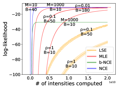
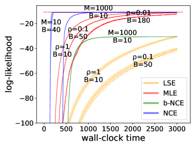
(b) Synthetic-2: $p^{*}$ and $p_{\theta}$ are of the same family.

Figure 1: Learning curves of MLE and NCE on synthetic datasets. The displayed $\rho$ and $M$ values are among the better ones that we found during hyperparameter search. The horizontal red line marks the highest held-out log-likelihood achieved by MLE. The shaded area of each curve shows the range of log-likelihood of three independent runs; most of them are too narrow to be easily noticed.

Ablation Study I: Always or Never Redraw Noise Samples. During training, for each observed data, we can choose to either redraw a new set of noise samples every time we train on it or keep reusing the old samples: we did the latter for Figure 1. In experiments doing the former, we observed better generation for tiny $M$ (e.g., $M=1$) but substantial slow-down (because of sampling) with no improved generalization for large $M$ (e.g, $1000$). Such results suggest that we always reuse old samples as long as $M$ is reasonably large: it is then what we do for all other experiments throughout the paper. See section D.4 for more details of this ablation study, including learning curves of the “always redraw” strategy in Figure 5.

5.2 Real-World Social Interaction Datasets with Large $K$

We also evaluate the methods on several real-world social interaction datasets that have many event types: see section D.1 for details (e.g, data statistics, pre-processing, data splits, etc). In this section, we show the learning curves on two particularly interesting datasets (explained below) in Figure 2 and leave those on the other datasets (which look similar) to section D.3.

EuroEmail (Paranjape et al., 2017). This dataset contains time-stamped emails between anonymized members of a European research institute. We work on a subset of $100$ most active members and then end up with $K=10000$ possible event types and $50000$ training event tokens.

BitcoinOTC (Kumar et al., 2016). This dataset contains time-stamped rating (positive/negative) records between anonymized users on the BitcoinOTC trading platform. We work on a subset of 100 most active users and then end up with $K=19800$ (self-rating not allowed) possible event types but only $1000$ training event tokens: this is an extremely data-sparse setting.

On these datasets, our model $p_{\theta}$ is still a neural Hawkes process. For the noise distribution $q$, we experiment with not only the coarse-to-fine neural process with $C=1$ but also a homogeneous Poisson process. As shown in Figure 2, our NCE tends to perform better with the neural $q$: this is because a neural model can better fit the data and thus provide better training signals, analogous to how a good generator can benefit the discriminator in the generative adversarial framework (Goodfellow et al., 2014). NCE with Poisson $q$ also shows benefits through the early and middle training stages, but it might suffer larger variance (e.g., Figure 2a2) and end up with slightly worse generalization (e.g., Figure 2b2). MLE with different $\rho$ values all eventually achieve the highest log-likelihood ($\approx-10$ on EuroEmail and $\approx-15$ on BitcoinOTC), but most of these runs are so slow that their peaks are out of the current views. The b-NCE runs with different $M$ values are slower, achieve worse generalization and suffer larger variance than our NCE; interestingly, b-NCE prefers Poisson $q$ to neural $q$ (better generalization on EuroEmail and smaller variance on BitcoinOTC). In general, LSE is the slowest, and the highest log-likelihood it can achieve ($\approx-30$ on EuroEmail and $\approx-25$ on BitcoinOTC) is lower than that of MLE and our NCE.

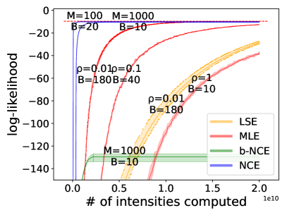
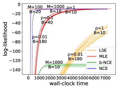
a1 EuroEmail: neural $q$

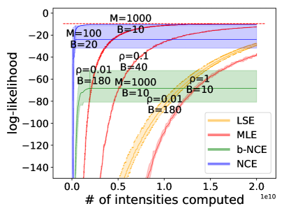
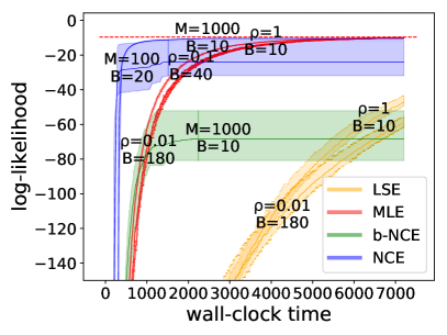
a2 EuroEmail: Poisson $q$

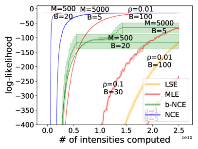
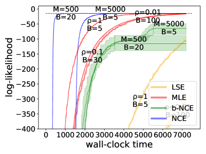
b1 BitcoinOTC: neural $q$.

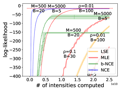
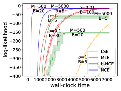
b2 BitcoinOTC: Poisson $q$.

Figure 2: Learning curves of MLE and NCE on the real-world social interaction datasets.

Ablation Study II: Trained vs. Untrained $q$. The noise distributions (except the ground-truth $q$ for Synthetic-1) that we have used so far were all pretrained on the same data as we train $p_{\theta}$. The training cost is cheap: e.g., on the datasets in this section, the actual wall-clock training time for the neural $q$ is less than 2% of what is needed to train $p_{\theta}$, and training the Poisson $q$ costs even less. We also experimented with untrained noise distributions and they were observed to perform worse (e.g., worse generalization, slower convergence and larger variance). See section D.5 for more details, including learning curves (Figure 6).

5.3 Real-World Dataset with Dynamic Facts

In this section, we let $p_{\theta}$ be a neural Datalog through time (NDTT) model (Mei et al., 2020). Such a model can be used in a domain in which new events dynamically update the set of event types and the structure of their intensity functions. We evaluate our method on training the domain-specific models presented by Mei et al. (2020), on the same datasets they used:

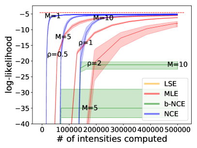
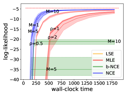
(a) RoboCup: $C=5$

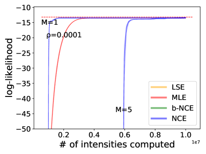
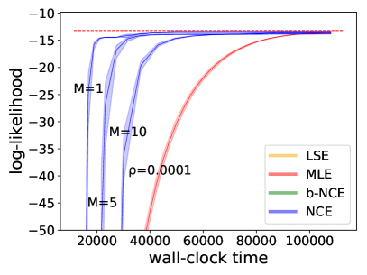
(b) IPTV: $C=49$

Figure 3: Learning curves of MLE and NCE on RoboCup and IPTV datasets.

RoboCup (Chen & Mooney, 2008). This dataset logs actions of robot players during RoboCup soccer games. The set of possible event types dynamically changes over time (e.g., only ball possessor can kick or pass) as the ball is frequently transferred between players (by passing or stealing). There are $K=528$ event types over all time, but only about $20$ of them are possible at any given time.

IPTV (Xu et al., 2018). This dataset contains time-stamped records of 1000 users watching 49 TV programs over 2012. The users are not able to watch a program until it is released, so the number of event types grows from $K=0$ to $K=49000$ as programs are released one after another.

The learning curves are displayed in Figure 3. On RoboCup, NCE only progresses faster than MLE at the early to middle training stages: $M=5$ and $M=10$ eventually achieved the highest log-likelihood at the same time as MLE and $M=1$ ended up with worse generalization. On IPTV, NCE with $M=1$ turned out to learn as well as and much faster than MLE. The dynamic architecture makes it hard to parallelize the intensity computation; MLE in particular performs poorly in wall-clock time, and we needed a remarkably small $\rho$ to let MLE finish within the shown time range. On both datasets, b-NCE and LSE drastically underperform MLE and NCE: their learning curves increase so slowly and achieve such poor generalization that only b-NCE with $M=5$ and $M=10$ are visible on the graphs.

Ablation Study III: Effect of $C$. In the above figures, we used the coarse-to-fine neural model as $q$. On RoboCup, each action (kick, pass, etc.) has a coarse-grained intensity, so $C=5$. On IPTV, we partition the event vocabulary by TV program, so $C=49$. We also experimented with $C=1$: this reduces the number of intensities computed during sampling on both datasets, but has (slightly) worse generalization on RoboCup (since $q$ becomes less expressive). See section D.6 for more details, including learning curves (Figure 7).

6 Conclusion

We have introduced a novel instantiation of the general NCE principle for training a multivariate point process model. Our objective has the same optimal parameters as the log-likelihood objective (if the model is well-specified), but needs fewer expensive function evaluations and much less wall-clock time in practice. This benefit is demonstrated on several synthetic and real-world datasets. Moreover, our method is provably consistent and efficient under mild assumptions.

Broader Impact

Our method is designed to train a multivariate point process for probabilistic modeling of event streams. By describing this method and releasing code, we hope to facilitate probabilistic modeling of continuous-time sequential data in many domains. Good probabilistic models make it possible to impute missing events, anticipate possible future events, and react accordingly. They can also be used in exploratory data analysis.

In addition to making it more feasible and more convenient for domain experts to train complex models with many event types, our method reduces the energy cost necessary to do so.

Examples of event streams with potential social impact include a person’s detailed food/exercise/sleep/medical event log, their social media interactions, their interactions with educational exercises or games, or their educational or workplace events (for time management and career planning); a customer’s interactions with a particular company or its website or other user interface; a company’s sales and purchases; geopolitical events, financial events, human activity modeling, music modeling, and dynamic resource requests.

We are not aware of any negative broader impacts that might stem from publishing this work.

Disclosure of Funding Sources

This work was supported by a Ph.D. Fellowship Award to the first author by Bloomberg L.P. and a National Science Foundation Grant No. 1718846 to the last author, as well as two Titan X Pascal GPUs donated by NVIDIA Corporation and compute cycles from the Maryland Advanced Research Computing Center.

Appendix A Proof Details for MLE

In this section, we prove the claim in section 2.2 that $\operatorname{argmax}_{\theta}J_{\mathrm{LL}}(\theta)=\Theta^{*}\mathrel{\stackrel{{\scriptstyle\textnormal{\tiny def}}}{{=}}}\{\theta^{*}:p_{\theta^{*}}=p^{*}\}$. For this purpose, we first rearrange $J_{\mathrm{LL}}(\theta)=\mathbb{E}_{{p^{*}(x_{[0,T)})}}\left[\log p_{\theta}(x_{[0,T)})\right]$ as below:

$$\sum_{x_{[0,T)}}p^{*}(x_{[0,T)})\log p_{\theta}(x_{[0,T)})$$ (8a)

$$= \int_{t=0}^{T}\sum_{x_{[0,t)}}p^{*}(x_{[0,t)}){\underbrace{\sum_{x_{[t,t+dt)}}p^{*}(x_{[t,t+dt)}\mid x_{[0,t)})\log p_{\theta}(x_{[t,t+dt)}\mid x_{[0,t)})}_{\text{call it }H_{\theta}(t,x_{[0,t)})}}$$ (8b)

The intuition for equation 8b is that due to the form of the autoregressive model, $\log p_{\theta}(x_{[0,T)})$ in equation 8a can be broken up into a sum of log (infinitesimal) probabilities of $x_{[t,t+dt)}$ on the infinitesimal intervals $[t,t+dt)$, each probability being conditioned on the past history $x_{[0,t)}$. When we take the expectation under $p^{*}$, each summand gets weighted by the probability that $x_{[0,t)}$ and $x_{[t,t+dt)}$ would take on the values in that summand. This gives a form (8b) that aggregates the infinitesimal quantities $H_{\theta}(t,x_{[0,t)})$ over possible times $t\in[0,T)$ and possible histories $x_{[0,t)}$.

Proof.

We first observe that $H_{\theta}(t,x_{[0,t)})$ is the negative cross-entropy between the conditional distributions of $p^{*}$ and $p_{\theta}$ at time $t$ (both conditioned on history $x_{[0,t)}$). Technically, $x_{[t,t+dt)}$ will have an event of type $k$ with probability $\lambda^{*}_{{k}}(t)dt$ under $p^{*}$ ($\lambda_{{k}}(t)dt$ under $p_{\theta}$) or has no event at all with probability $1-\sum_{k=1}^{K}\lambda^{*}_{{k}}(t)dt$ under $p^{*}$ ($1-\sum_{k=1}^{K}\lambda_{{k}}(t)dt$ under $p_{\theta}$). So the term $H_{\theta}(t,x_{[0,t)})$ is actually the negative cross entropy between the following two discrete distributions over $\{\varnothing,1,\ldots,K\}$:

$$\left[\left(1-\sum_{k=1}^{K}\lambda^{*}_{{k}}(t\mid x_{[0,t)})dt\right),\;\lambda^{*}_{{1}}(t\mid x_{[0,t)})dt,\;\ldots\;,\;\lambda^{*}_{{K}}(t\mid x_{[0,t)})dt\right]$$ (9a)

$$\left[\left(1-\sum_{k=1}^{K}\lambda_{{k}}(t\mid x_{[0,t)})dt\right),\;\lambda_{{1}}(t\mid x_{[0,t)})dt,\;\ldots\;,\;\lambda_{{K}}(t\mid x_{[0,t)})dt\right]$$ (9b)

The (infinitesimal) negative cross-entropy between them is always smaller than or equal to the negative entropy of the distribution in equation 9a: it will be strictly smaller if these two distributions are distinct, and equal when they are identical.

It is then obvious that any $\theta^{*}\in\Theta^{*}$ maximizes $J_{\mathrm{LL}}(\theta)$ because it maximizes the negative cross-entropy for any history $x_{[0,t)}$ at any time $t$.

To check if any other $\bar{\theta}\notin\Theta^{*}$ maximizes $J_{\mathrm{LL}}(\theta)$ as well, we analyze

$$J_{\mathrm{LL}}(\bar{\theta})-J_{\mathrm{LL}}(\theta^{*})=\int_{t=0}^{T}\sum_{x_{[0,t)}}p^{*}(x_{[0,t)}){\underbrace{(H_{\bar{\theta}}({t},{x}_{[0,{t})})-H_{\theta^{*}}({t},{x}_{[0,{t})}))}_{\text{denote it as }G_{\bar{\theta}}(t,x_{[0,t)})dt}}$$ (10)

where $\theta^{*}$ can be any member in $\Theta^{*}$. Note that we can denote $H_{\bar{\theta}}-H_{\theta^{*}}$ as $G_{\bar{\theta}}dt$ because the probabilities in $H$ and thus the entropy changes (if any) are all infinitesimal.

According to the definition of $\bar{\theta}$ and $\theta^{*}$, there must exist a stream $\bar{x}_{[0,T)}$, a time $\bar{t}\in(0,T)$ and a type $\bar{k}\in\{1,\ldots,K\}$ such that $\lambda_{{\bar{k}}}(\bar{t}\mid\bar{x}_{[0,\bar{t})})\neq\lambda^{*}_{{\bar{k}}}(\bar{t}\mid\bar{x}_{[0,\bar{t})})$. Therefore, we have $G_{\bar{\theta}}(\bar{t},\bar{x}_{[0,\bar{t})})<0$ since the distributions in equation 9 are distinct for the given history $\bar{x}_{[0,\bar{t})}$. Does this difference lead to any overall change of the entire objective?

Actually, according to Lemma 1 (that we will prove shortly), the existence of such $\bar{x}_{[0,T)}$, $\bar{t}$ and $\bar{k}$ implies that there exists an interval $(t^{\prime},t^{\prime\prime})\subset[0,T)$ such that, for any $t\in(t^{\prime},t^{\prime\prime})$, there exists a set $\mathcal{X}(t)$ of histories with non-zero measure such that any $x_{[0,t)}\in\mathcal{X}(t)$ satisfies $\lambda_{{\bar{k}}}({t}\mid{x}_{[0,{t})})\neq\lambda^{*}_{{\bar{k}}}({t}\mid{x}_{[0,{t})})$. That is to say, the fraction of the integral over $(t^{\prime},t^{\prime\prime})$ is a non-infinitesimal negative number:

$$\int_{t=t^{\prime}}^{t^{\prime\prime}}\sum_{x_{[0,t)}}p^{*}(x_{[0,t)})G_{\bar{\theta}}(t,x_{[0,t)})dt$$ (11a)

$$= {\underbrace{\int_{t=t^{\prime}}^{t^{\prime\prime}}\sum_{x_{[0,t)}\in\mathcal{X}(t)}p^{*}(x_{[0,t)})G_{\bar{\theta}}(t,x_{[0,t)})dt}_{<0}}+{\underbrace{\int_{t=t^{\prime}}^{t^{\prime\prime}}\sum_{x_{[0,t)}\notin\mathcal{X}(t)}p^{*}(x_{[0,t)})G_{\bar{\theta}}(t,x_{[0,t)})dt}_{\leq 0}}$$ (11b)

where the second integral $\leq 0$ because $G_{\theta}$ always $\leq 0$. For the same reason, we also have $\int_{t=0}^{t^{\prime}}\sum_{x_{[0,t)}}p^{*}(x_{[0,t)})G_{\bar{\theta}}(t,x_{[0,t)})dt\leq 0$ and $\int_{t=t^{\prime\prime}}^{T}\sum_{x_{[0,t)}}p^{*}(x_{[0,t)})G_{\bar{\theta}}(t,x_{[0,t)})dt\leq 0$. Then the overall difference must be strictly negative, i.e.,

$$J_{\mathrm{LL}}(\bar{\theta})-J_{\mathrm{LL}}(\theta^{*})<0$$ (12)

Note that this inequality holds for any $\bar{\theta}\notin\Theta^{*}$ and any $\theta^{*}\in\Theta^{*}$, meaning that $\theta^{*}\in\Theta^{*}$ is necessary to maximize the objective.

Now the proof of $\operatorname{argmax}_{\theta}J_{\mathrm{LL}}(\theta)=\Theta^{*}$ is complete.

∎

Lemma 1.

Suppose that we have two intensity functions that meet assumption 1: they have different parameters $\theta$ and $\theta^{*}$ and are denoted as $\lambda_{{k}}(t\mid x_{[0,t)})$ and $\lambda^{*}_{{k}}(t\mid x_{[0,t)})$ respectively. If there exists a stream $\bar{x}_{[0,T)}$, a time $\bar{t}\in(0,T)$ and a type $\bar{k}\in\{1,\ldots,K\}$ such that $\lambda_{{\bar{k}}}(\bar{t}\mid\bar{x}_{[0,\bar{t})})\neq\lambda^{*}_{{\bar{k}}}(\bar{t}\mid\bar{x}_{[0,\bar{t})})$, then there exists an open interval $(t^{\prime},t^{\prime\prime})\subset[0,T)$ such that, for any $t\in(t^{\prime},t^{\prime\prime})$, there exists a set $\mathcal{X}$ of histories with non-zero measure such that any $x_{[0,t)}\in\mathcal{X}$ satisfies $\lambda_{{\bar{k}}}({t}\mid{x}_{[0,{t})})\neq\lambda^{*}_{{\bar{k}}}({t}\mid{x}_{[0,{t})})$.

This lemma says: if $\theta$ and $\theta^{*}$ are meaningfully different in that they predict different intensities at time $t$ for some history, then they actually do so for a set of histories of non-zero measure, making this difference visible in the objective functions like $J_{\mathrm{LL}}(\theta)$ (see above) and $J_{\mathrm{NC}}(\theta)$ (see Appendix B). Note that previous work did not encounter this since they only worked on either non-sequential data (e.g., Gutmann & Hyvärinen (2010, 2012)) or discrete-time sequential data (e.g., Ma & Collins (2018)).

Proof.

We first prove the existence of an interval $(t^{\prime},t^{\prime\prime})$ such that $\lambda_{{\bar{k}}}({t}\mid\bar{x}_{[0,{t})})\neq\lambda^{*}_{{\bar{k}}}({t}\mid\bar{x}_{[0,{t})})$ for the given stream $\bar{x}_{[0,T)}$ and any time $t\in(t^{\prime},t^{\prime\prime})$. It turns out to be straightforward under assumption 1: since the intensity functions are continuous between events, we can construct this interval by expanding from the given time $\bar{t}$ until $\lambda_{{\bar{k}}}({t}\mid\bar{x}_{[0,{t})})=\lambda^{*}_{{\bar{k}}}({t}\mid\bar{x}_{[0,{t})})$.

We use $d$ to denote the maximal difference between the intensities over $(t^{\prime},t^{\prime\prime})$, i.e., $d\mathrel{\stackrel{{\scriptstyle\textnormal{\tiny def}}}{{=}}}\max_{t\in(t^{\prime},t^{\prime\prime})}|\lambda_{{\bar{k}}}({t}\mid\bar{x}_{[0,{t})})-\lambda^{*}_{{\bar{k}}}({t}\mid\bar{x}_{[0,{t})})|$. Then, to facilitate the rest of the proof, we shrink the interval $(t^{\prime},t^{\prime\prime})$ such that $|\lambda_{{\bar{k}}}({t}\mid\bar{x}_{[0,{t})})-\lambda^{*}_{{\bar{k}}}({t}\mid\bar{x}_{[0,{t})})|>d/2$ for any time $t\in(t^{\prime},t^{\prime\prime})$.

Now, for any time $t\in(t^{\prime},t^{\prime\prime})$, we prove the existence of the set described in Lemma 1 by constructing it.

We initialize this set as $\{\bar{x}_{[0,t)}\}$. If $\bar{x}_{[0,t)}$ doesn’t have any event, then its probability $p(\bar{x}_{[0,{t})})=\exp(-\int_{s=0}^{{t}}\sum_{k=1}^{K}{\lambda}_{k}(s\mid\bar{x}_{[0,s)})ds)$ is not infinitesimal and this set already has non-zero measure.

What if $\bar{x}_{[0,t)}$ has $I\geq 1$ events at times $0<t_{1}<\ldots<t_{I}<t$? Intuitively, we can construct many other histories satisfying the intensity inequality by slightly shifting the time of each event: as long as they aren’t shifted by too far, the $d/2$ difference between intensities won’t vanish (even if it decreases). See the formal proof as below.

In the case of $I\geq 1$, the probability $p(\bar{x}_{[0,{t})})$ is infinitesimal in the order of $(dt)^{I}$: $p(\bar{x}_{[0,{t})})=\prod_{i=1}^{I}(\lambda_{{\bar{x}_{t_{i}}}}(t_{i}\mid\bar{x}_{[0,t_{i})})dt)\exp(-\int_{s=0}^{{t}}\sum_{k=1}^{K}{\lambda}_{k}(s\mid\bar{x}_{[0,s)})ds)$. Therefore, to construct a set with non-zero measure, the number of histories satisfying the inequality has to be in the order of $(\tfrac{1}{dt})^{I}$.

We define an open interval $(t^{\prime}_{1},t^{\prime\prime}_{1})$ that covers $t_{1}$ but not any other event time. Now we can construct uncountably many—in the order of $\tfrac{1}{dt}$—histories $x_{[0,t)}$ by freely shifting the event time $t_{1}$ inside $(t^{\prime}_{1},t^{\prime\prime}_{1})$. Suppose that $t_{1}$ has been shifted by $\Delta\in\mathbb{R}$. Under assumption 1, there is a continuous function $c(\Delta)$ such that $c(0)=0$ and

$$\lambda_{{\bar{k}}}({t}\mid x_{[0,t)})-\lambda^{*}_{{\bar{k}}}({t}\mid x_{[0,t)})=\lambda_{{\bar{k}}}({t}\mid\bar{x}_{[0,{t})})-\lambda^{*}_{{\bar{k}}}({t}\mid\bar{x}_{[0,{t})})+c(\Delta)$$ (13)

meaning that the intensity difference will change by $c(\Delta)$. By triangle inequality, we have

$$\left|\lambda_{{\bar{k}}}({t}\mid x_{[0,t)})-\lambda^{*}_{{\bar{k}}}({t}\mid x_{[0,t)})\right|\geq\left|\left|\lambda_{{\bar{k}}}({t}\mid\bar{x}_{[0,{t})})-\lambda^{*}_{{\bar{k}}}({t}\mid\bar{x}_{[0,{t})})\right|-\left|c(\Delta)\right|\right|$$ (14)

Since $c(\Delta)$ is continuous, as long as we make $\left|\Delta\right|$ small enough, we’ll have $\left|c(\Delta)\right|\leq d/2$ and then the following inequality holds:

$$\left|\lambda_{{\bar{k}}}({t}\mid x_{[0,t)})-\lambda^{*}_{{\bar{k}}}({t}\mid x_{[0,t)})\right|\geq\left|\lambda_{{\bar{k}}}({t}\mid\bar{x}_{[0,{t})})-\lambda^{*}_{{\bar{k}}}({t}\mid\bar{x}_{[0,{t})})\right|-\left|c(\Delta)\right|>d/2-d/2=0$$ (15)

meaning that the intensities given the new history are still different. Therefore, as long as we keep the interval $(t^{\prime}_{1},t^{\prime\prime}_{1})$ small enough, we’ll have order-$\tfrac{1}{dt}$ many histories and the inequality in equation 15 holds given any of them.

Recall that we need order-$(\tfrac{1}{dt})^{I}$ many such histories. We can obtain them by simply defining $I$ disjoint open intervals $(t^{\prime}_{1},t^{\prime\prime}_{1}),\ldots,(t^{\prime}_{I},t^{\prime\prime}_{I})$ such that $t_{i}\in(t^{\prime}_{i},t^{\prime\prime}_{i})$ and freely shifting each event time $t_{i}$ inside $(t^{\prime}_{i},t^{\prime\prime}_{i})$. Suppose that $t_{i}$ has been shifted by $\Delta_{i}\in\mathbb{R}$, Under assumption 1, there is a continuous function $c(\Delta_{1},\ldots,\Delta_{I})$ such that $c(0,\ldots,0)=0$ and

$$\lambda_{{\bar{k}}}({t}\mid x_{[0,t)})-\lambda^{*}_{{\bar{k}}}({t}\mid x_{[0,t)})=\lambda_{{\bar{k}}}({t}\mid\bar{x}_{[0,{t})})-\lambda^{*}_{{\bar{k}}}({t}\mid\bar{x}_{[0,{t})})+c(\Delta_{1},\ldots,\Delta_{I})$$ (16)

Since $c$ is a continuous function, there exist $I$ positive real numbers $\bar{\Delta}_{1},\ldots,\bar{\Delta}_{I}$ such that $\left|c(\Delta_{1},\ldots,\Delta_{I})\right|\leq d/2$ as long as $\left|\Delta_{i}\right|\leq\bar{\Delta}_{i}$ holds for all $i=1,\ldots,I$. In this case, by triangle inequality, we still have

$$\left|\lambda_{{\bar{k}}}({t}\mid x_{[0,t)})-\lambda^{*}_{{\bar{k}}}({t}\mid x_{[0,t)})\right|\geq\left|\lambda_{{\bar{k}}}({t}\mid\bar{x}_{[0,{t})})-\lambda^{*}_{{\bar{k}}}({t}\mid\bar{x}_{[0,{t})})\right|-\left|\Delta_{i}\right|>0$$ (17)

Now we have order-$(\tfrac{1}{dt})^{I}$ many histories: each of them has order-$(dt)^{I}$ probability and the inequality in equation 17 holds given any of them. That is to say, the set of these histories has non-zero measure and we have $\lambda_{{\bar{k}}}({t}\mid x_{[0,t)})\neq\lambda^{*}_{{\bar{k}}}({t}\mid x_{[0,t)})$ given any $x_{[0,t)}$ in this set.

This completes the proof.

∎

Appendix B NCE Details

In this section, we will discuss the theoretical guarantees of our NCE method in detail.

B.1 Derivation Details

In this section, we show how to get the rearranged NCE objective in section 3.3 from equation 6.

First of all, we observe that:

$$\mathbb{E}_{{x_{[0,T)}^{0}\sim p^{*},x_{[0,T)}^{1:M}\sim q}}\left[\sum_{t:x_{t}^{0}\neq\varnothing}\log\tfrac{\lambda_{{x_{t}^{0}}}(t\mid x_{[0,t)}^{0})}{\underline{\lambda}_{x_{t}^{0}}(t\mid x_{[0,t)}^{0})}+\sum_{m=1}^{M}\sum_{t:x_{t}^{m}\neq\varnothing}\log\tfrac{\lambda^{\mathrm{q}}_{{x_{t}^{m}}}(t\mid x_{[0,t)}^{0})}{\underline{\lambda}_{x_{t}^{m}}(t\mid x_{[0,t)}^{0})}\right]$$ (18a)

$$= \int_{t=0}^{T}\mathbb{E}_{{x_{[0,t)}^{0}\sim p^{*}}}\left[\sum_{k=1}^{K}\lambda^{*}_{{k}}(t\mid x_{[0,t)}^{0})dt\log\tfrac{\lambda_{{x_{t}^{0}}}(t\mid x_{[0,t)}^{0})}{\underline{\lambda}_{x_{t}^{0}}(t\mid x_{[0,t)}^{0})}+\sum_{m=1}^{M}\sum_{k=1}^{K}\lambda^{\mathrm{q}}_{{k}}(t\mid x_{[0,t)}^{0})dt\log\tfrac{\lambda^{\mathrm{q}}_{{x_{t}^{m}}}(t\mid x_{[0,t)}^{0})}{\underline{\lambda}_{x_{t}^{m}}(t\mid x_{[0,t)}^{0})}\right]$$ (18b)

This rearrangement is similar to that of equations 8a–8b. The intuition of equation 18a is that we sample $M$ i.i.d. noise streams $x_{[0,T)}^{1},\ldots,x_{[0,T)}^{M}$ for each possible real data $x_{[0,T)}^{0}$, sum up the log-ratio whenever ${x}_{t}^{0:M}$ has an event, and then take the expectation over all the possible real data $x_{[0,T)}^{0}$. The intuition of equation 18b is that we draw noise samples $x_{t}^{1},\ldots,x_{t}^{M}$ for each real history $x_{[0,t)}^{0}$ at each time $t$, compute the log-ratio if ${x}_{t}^{0:M}$ has an event, take the expectation of the log-ratio over all the possible real histories and then sum over all the possible times. Therefore, these two expectations are equal.

We further rearrange equation 18 as

$$=\int_{t=0}^{T}\mathbb{E}_{{x_{[0,t)}^{0}\sim p^{*}}}\left[\sum_{k=1}^{K}\left(\lambda^{*}_{{k}}(t\mid x_{[0,t)}^{0})dt\log\tfrac{\lambda_{{k}}(t\mid x_{[0,t)}^{0})}{\underline{\lambda}_{k}(t\mid x_{[0,t)}^{0})}+\sum_{m=1}^{M}\lambda^{\mathrm{q}}_{{k}}(t\mid x_{[0,t)}^{0})dt\log\tfrac{\lambda^{\mathrm{q}}_{{k}}(t\mid x_{[0,t)}^{0})}{\underline{\lambda}_{k}(t\mid x_{[0,t)}^{0})}\right)\right]$$ (19a)

$$= \int_{t=0}^{T}\mathbb{E}_{{x_{[0,t)}^{0}\sim p^{*}}}\left[\sum_{k=1}^{K}\left(\lambda^{*}_{{k}}(t\mid x_{[0,t)}^{0})dt\log\tfrac{\lambda_{{k}}(t\mid x_{[0,t)}^{0})}{\underline{\lambda}_{k}(t\mid x_{[0,t)}^{0})}+M\lambda^{\mathrm{q}}_{{k}}(t\mid x_{[0,t)}^{0})dt\log\tfrac{\lambda^{\mathrm{q}}_{{k}}(t\mid x_{[0,t)}^{0})}{\underline{\lambda}_{k}(t\mid x_{[0,t)}^{0})}\right)\right]$$ (19b)

$$= \int_{t=0}^{T}\mathbb{E}_{{x_{[0,t)}^{0}\sim p^{*}}}\left[\sum_{k=1}^{K}\underline{\lambda}^{*}_{k}(t\mid x_{[0,t)}^{0})dt\left(\tfrac{\lambda^{*}_{{k}}(t\mid x_{[0,t)}^{0})}{\underline{\lambda}^{*}_{k}(t\mid x_{[0,t)}^{0})}\log\tfrac{\lambda_{{k}}(t\mid x_{[0,t)}^{0})}{\underline{\lambda}_{k}(t\mid x_{[0,t)}^{0})}+M\tfrac{\lambda^{\mathrm{q}}_{{k}}(t\mid x_{[0,t)}^{0})}{\underline{\lambda}^{*}_{k}(t\mid x_{[0,t)}^{0})}\log\tfrac{\lambda^{\mathrm{q}}_{{k}}(t\mid x_{[0,t)}^{0})}{\underline{\lambda}_{k}(t\mid x_{[0,t)}^{0})}\right)\right]$$ (19c)

where $\underline{\lambda}^{*}_{k}(t\mid x_{[0,t)}^{0})\mathrel{\stackrel{{\scriptstyle\textnormal{\tiny def}}}{{=}}}\lambda^{*}_{{k}}(t\mid x_{[0,t)}^{0})+M\lambda^{\mathrm{q}}_{{k}}(t\mid x_{[0,t)}^{0})$ can be thought of as the intensity of type $k$ under the superposition of $p^{*}$ and $M$ copies of $q$.

Now we obtain the final rearranged objective:

$$\int_{t=0}^{T}\sum_{x_{[0,t)}^{0}}p^{*}(x_{[0,t)}^{0})\sum_{k=1}^{K}\underline{\lambda}^{*}_{k}(t\mid x_{[0,t)}^{0}){\underbrace{\left(\tfrac{{\lambda}^{*}_{k}(t\mid x_{[0,t)}^{0})}{\underline{\lambda}^{*}_{k}(t\mid x_{[0,t)}^{0})}\log\tfrac{{\lambda}_{k}(t\mid x_{[0,t)}^{0})}{\underline{\lambda}_{k}(t\mid x_{[0,t)}^{0})}+M\tfrac{{\lambda}^{q}_{k}(t\mid x_{[0,t)}^{0})}{\underline{\lambda}^{*}_{k}(t\mid x_{[0,t)}^{0})}\log\tfrac{{\lambda}^{q}_{k}(t\mid x_{[0,t)}^{0})}{\underline{\lambda}_{k}(t\mid x_{[0,t)}^{0})}\right)}_{\text{call it }H_{\theta}(k,t,x_{[0,t)}^{0})}}dt$$ (20)

B.2 Optimality Proof Details

In this section, we prove Theorem 1 that we stated in section 3.3. Recall the theorem: See 1

We first need to highlight the key insight that $H_{\theta}(k,t,x_{[0,t)}^{0})$ in equation 20 is the negative cross-entropy between the following two discrete distributions over $\{\varnothing,1,\ldots,K\}$:

$$[\tfrac{{\lambda}^{*}_{k}(t\mid x_{[0,t)}^{0})}{\underline{\lambda}^{*}_{k}(t\mid x_{[0,t)}^{0})},\tfrac{{\lambda}^{q}_{k}(t\mid x_{[0,t)}^{0})}{\underline{\lambda}^{*}_{k}(t\mid x_{[0,t)}^{0})},\ldots,\tfrac{{\lambda}^{q}_{k}(t\mid x_{[0,t)}^{0})}{\underline{\lambda}^{*}_{k}(t\mid x_{[0,t)}^{0})}]$$ (21a)

$$[\tfrac{{\lambda}_{k}(t\mid x_{[0,t)}^{0})}{\underline{\lambda}_{k}(t\mid x_{[0,t)}^{0})},{\underbrace{\tfrac{{\lambda}^{q}_{k}(t\mid x_{[0,t)}^{0})}{\underline{\lambda}_{k}(t\mid x_{[0,t)}^{0})},\ldots,\tfrac{{\lambda}^{q}_{k}(t\mid x_{[0,t)}^{0})}{\underline{\lambda}_{k}(t\mid x_{[0,t)}^{0})}}_{\text{length is }M}}]$$ (21b)

This negative cross-entropy is always smaller than or equal to the negative entropy of the distribution in equation 21a: it will be strictly smaller if these two distributions are distinct and equal when they are identical. Notice that in contrast to the negative cross-entropy at equation 9, this negative cross-entropy here is not infinitesimal.

Proof.

The “if” part is straightforward to prove. Any $\theta$ for which $p_{\theta}=p^{*}$ would make ${\lambda}_{k}(t\mid x_{[0,t)}^{0})={\lambda}^{*}_{k}(t\mid x_{[0,t)}^{0})$, thus maximizing the negative cross-entropy between the two distributions in equation 21, for any type $k$ and any real history $x_{[0,t)}^{0}$ at any time $t$. Then the NCE objective in equation 20 is obviously maximized.

To check if any other $\bar{\theta}\notin\Theta^{*}\mathrel{\stackrel{{\scriptstyle\textnormal{\tiny def}}}{{=}}}\{\theta^{*}:p_{\theta^{*}}=p^{*}\}$ maximizes $J_{\mathrm{NC}}(\theta)$ as well, we analyze

$$J_{\mathrm{NC}}(\bar{\theta})-J_{\mathrm{NC}}(\theta^{*})=\int_{t=0}^{T}\sum_{x_{[0,t)}^{0}}p^{*}(x_{[0,t)}^{0})\sum_{k=1}^{K}\underline{\lambda}^{*}_{k}(t\mid x_{[0,t)}^{0}){\underbrace{\left(H_{\bar{\theta}}(k,t,x_{[0,t)}^{0})-H_{\theta^{*}}(k,t,x_{[0,t)}^{0})\right)}_{\text{denote it as }G_{\bar{\theta}}(k,t,x_{[0,t)}^{0})}}dt$$

where $\theta^{*}$ can be any member in $\Theta^{*}$. Note that $G_{\bar{\theta}}$ is not infinitesimal because the probabilities in $H$ and thus the entropy changes (if any) are not infinitesimal.

According to the definition of $\bar{\theta}$ and $\theta^{*}$, there must exist a stream $\bar{x}_{[0,T)}$, a time $\bar{t}\in(0,T)$ and a type $\bar{k}\in\{1,\ldots,K\}$ such that $\lambda_{{\bar{k}}}(\bar{t}\mid\bar{x}_{[0,\bar{t})})\neq\lambda^{*}_{{\bar{k}}}(\bar{t}\mid\bar{x}_{[0,\bar{t})})$. Therefore, we have $G_{\bar{\theta}}(\bar{k},\bar{t},\bar{x}_{[0,\bar{t})})<0$ since the distributions in equation 21 are distinct for the given history $\bar{x}_{[0,\bar{t})}$. Does this difference lead to any overall change of the entire objective?

Actually, according to Lemma 1 in Appendix A, the existence of such $\bar{x}_{[0,T)}$, $\bar{t}$ and $\bar{k}$ implies that there exists an interval $(t^{\prime},t^{\prime\prime})\subset[0,T)$ such that, for any $t\in(t^{\prime},t^{\prime\prime})$, there exists a set $\mathcal{X}(t)$ of histories with non-zero measure such that any $x_{[0,t)}\in\mathcal{X}(t)$ satisfies $\lambda_{{\bar{k}}}({t}\mid{x}_{[0,{t})})\neq\lambda^{*}_{{\bar{k}}}({t}\mid{x}_{[0,{t})})$. Then, given any of these histories, the entropy difference $G_{\bar{\theta}}$ would be $<0$. That is to say, the following integral must be a non-infinitesimal negative number:

$$\int_{t=0}^{T}\sum_{x_{[0,t)}^{0}}p^{*}(x_{[0,t)}^{0})\underline{\lambda}^{*}_{\bar{k}}(t\mid x_{[0,t)}^{0})G_{\bar{\theta}}(\bar{k},t,x_{[0,t)}^{0})dt$$ (22a)

$$= \int_{t=t^{\prime}}^{t^{\prime\prime}}\sum_{x_{[0,t)}^{0}\in\mathcal{X}(t)}p^{*}(x_{[0,t)}^{0})\underline{\lambda}^{*}_{\bar{k}}(t\mid x_{[0,t)}^{0})G_{\bar{\theta}}(\bar{k},t,x_{[0,t)}^{0})dt <0$$ ( ) (22b)

$$+ \int_{t=t^{\prime}}^{t^{\prime\prime}}\sum_{x_{[0,t)}^{0}\notin\mathcal{X}(t)}p^{*}(x_{[0,t)}^{0})\underline{\lambda}^{*}_{\bar{k}}(t\mid x_{[0,t)}^{0})G_{\bar{\theta}}(\bar{k},t,x_{[0,t)}^{0})dt \leq 0$$ ( ) (22c)

$$+ \int_{t=0}^{t^{\prime}}\sum_{x_{[0,t)}^{0}}p^{*}(x_{[0,t)}^{0})\underline{\lambda}^{*}_{\bar{k}}(t\mid x_{[0,t)}^{0})G_{\bar{\theta}}(\bar{k},t,x_{[0,t)}^{0})dt \leq 0$$ ( ) (22d)

$$+ \int_{t=t^{\prime\prime}}^{T}\sum_{x_{[0,t)}^{0}}p^{*}(x_{[0,t)}^{0})\underline{\lambda}^{*}_{\bar{k}}(t\mid x_{[0,t)}^{0})G_{\bar{\theta}}(\bar{k},t,x_{[0,t)}^{0})dt \leq 0$$ ( ) (22e)

Therefore, the overall difference must be $<0$ as well:

$$J_{\mathrm{LL}}(\bar{\theta})-J_{\mathrm{LL}}(\theta^{*}) =\int_{t=0}^{T}\sum_{x_{[0,t)}^{0}}p^{*}(x_{[0,t)}^{0})\sum_{k=1}^{K}\underline{\lambda}^{*}_{k}(t\mid x_{[0,t)}^{0})G_{\bar{\theta}}(k,t,x_{[0,t)}^{0})dt$$ (23a)

$$=\int_{t=0}^{T}\sum_{x_{[0,t)}^{0}}p^{*}(x_{[0,t)}^{0})\underline{\lambda}^{*}_{\bar{k}}(t\mid x_{[0,t)}^{0})G_{\bar{\theta}}(\bar{k},t,x_{[0,t)}^{0})dt <0$$ ( ) (23b)

$$+\int_{t=0}^{T}\sum_{x_{[0,t)}^{0}}p^{*}(x_{[0,t)}^{0})\sum_{k\neq\bar{k}}\underline{\lambda}^{*}_{k}(t\mid x_{[0,t)}^{0})G_{\bar{\theta}}(k,t,x_{[0,t)}^{0})dt \leq 0$$ ( ) (23c)

Note that $J_{\mathrm{LL}}(\bar{\theta})-J_{\mathrm{LL}}(\theta^{*})<0$ holds any $\bar{\theta}\notin\Theta^{*}$ and any $\theta^{*}\in\Theta^{*}$, meaning that $\theta^{*}\in\Theta^{*}$ is necessary to maximize the objective. Then the proof of the “only if” part is complete.

Now we have proved both the “if” and “only if” parts so the proof is complete.

∎

B.3 Consistency Proof Details

To discuss the statistical consistency (in this section) and efficiency (in section B.4), we first need to spell out the empirical version of the objective

$$J_{\mathrm{NC}}^{N}(\theta) =\tfrac{1}{N}\sum_{n=1}^{N}\left(\sum_{t:x_{t,n}^{0}\neq\varnothing}\log\tfrac{\lambda_{{x_{t,n}^{0}}}(t\mid x_{[0,t),n}^{0})}{\underline{\lambda}_{x_{t,n}^{0}}(t\mid x_{[0,t),n}^{0})}+\sum_{m=1}^{M}\sum_{t:x_{t,n}^{m}\neq\varnothing}\log\tfrac{\lambda^{\mathrm{q}}_{{x_{t,n}^{m}}}(t\mid x_{[0,t),n}^{0})}{\underline{\lambda}_{x_{t,n}^{m}}(t\mid x_{[0,t),n}^{0})}\right)$$ (24)

where the subscript _n denotes the $n$^th i.i.d. draw of the observed sequence and the $M$ noise samples for this sequence. It is obvious that $\lim_{N\rightarrow\infty}J_{\mathrm{NC}}^{N}(\theta)\rightarrow J_{\mathrm{NC}}(\theta)$.

To analyze the consistency, we make the following assumptions:

Assumption 3 (Continuity wrt. $\theta$).

For any history $x_{[0,t)}$ and event type $k\in\{1,\ldots,K\}$, $\lambda_{{k}}(t\mid x_{[0,t)})$ is continuous with respect to $\theta$.

Assumption 4 (Compactness).

The set of optimal parameters $\Theta^{*}$ is contained in the interior of a compact set $\Theta\subset\mathbb{R}^{|\theta|}$.

They are analogous to assumptions 4.2 and 4.3 of Ma & Collins (2018) respectively.

Our NCE method turns out to be strongly consistent in the sense that:

Theorem 2 (Consistency).

Under assumptions 3, 2 and 4, for any $\theta\in\Theta_{\text{NC}}^{N}\mathrel{\stackrel{{\scriptstyle\textnormal{\tiny def}}}{{=}}}\operatorname{argmax}_{\theta}J_{\mathrm{NC}}^{N}(\theta)$ and $M\geq 1$, with probability 1, we have $\lim_{N\rightarrow\infty}\min_{\theta^{*}\in\Theta^{*}}\|\theta-\theta^{*}\|=0$ where $\|\cdot\|$ is the L₂ norm.

The intuition of this theorem is that: since the two functions $J_{\mathrm{NC}}^{N}(\theta)$ and $J_{\mathrm{NC}}(\theta)$ will become the same as $N\rightarrow\infty$ and they are continuous with respect to $\theta$, then any $\theta\in\operatorname{argmax}_{\theta}J_{\mathrm{NC}}^{N}(\theta)$ has to be close to some member of the set $\operatorname{argmax}_{\theta}J_{\mathrm{NC}}(\theta)$. The full proof is almost identical to the proof of Theorem 4.2 in Ma & Collins (2018). But we will still spell it out in our notation for completeness.

Proof.

Under the assumption in Theorem 2, by classical large sample theory (Ferguson, 1996), we have

$$\mathbb{P}\left[\lim_{N\rightarrow\infty}\sup_{\theta\in\Theta^{\prime}}|J_{\mathrm{NC}}^{N}(\theta)-J_{\mathrm{NC}}(\theta)|=0\right]=1\text{ for any compact set }\Theta^{\prime}\subset\Theta$$ (25)

where $\mathbb{P}$ stands for “probability”. Since $|J_{\mathrm{NC}}^{N}(\theta)-J_{\mathrm{NC}}(\theta)|\geq J_{\mathrm{NC}}^{N}(\theta)-J_{\mathrm{NC}}(\theta)$, we have

$$\mathbb{P}\left[\limsup_{N\rightarrow\infty}\sup_{\theta\in\Theta^{\prime}}(J_{\mathrm{NC}}^{N}(\theta)-J_{\mathrm{NC}}(\theta))\leq 0\right]=1$$ (26)

Moreover, for any $\theta^{\prime N}\in\operatorname{argmax}_{\theta\in\Theta^{\prime}}J_{\mathrm{NC}}^{N}(\theta)$, we have

$$\sup_{\theta\in\Theta^{\prime}}(J_{\mathrm{NC}}^{N}(\theta)-J_{\mathrm{NC}}(\theta))\geq J_{\mathrm{NC}}^{N}(\theta^{\prime N})-J_{\mathrm{NC}}(\theta^{\prime N})\geq\sup_{\theta\in\Theta^{\prime}}J_{\mathrm{NC}}^{N}(\theta)-\sup_{\theta\in\Theta^{\prime}}J_{\mathrm{NC}}(\theta)$$ (27)

Plugging equation 27 into equation 26 gives

$$\mathbb{P}\left[\limsup_{N\rightarrow\infty}\sup_{\theta\in\Theta^{\prime}}J_{\mathrm{NC}}^{N}(\theta)-\sup_{\theta\in\Theta^{\prime}}J_{\mathrm{NC}}(\theta)\leq 0\right]=\mathbb{P}\left[\limsup_{N\rightarrow\infty}\sup_{\theta\in\Theta^{\prime}}J_{\mathrm{NC}}^{N}(\theta)\leq\sup_{\theta\in\Theta^{\prime}}J_{\mathrm{NC}}(\theta)\right]=1$$ (28)

For any $\delta>0$, we define $\Theta_{\delta}\mathrel{\stackrel{{\scriptstyle\textnormal{\tiny def}}}{{=}}}\{\theta:\min_{\theta^{*}\in\Theta^{*}}\|\theta-\theta^{*}\|>\delta\}$ and have

$$\mathbb{P}\left[\limsup_{N\rightarrow\infty}\sup_{\theta\in\Theta_{\delta}}J_{\mathrm{NC}}^{N}(\theta)\leq\sup_{\theta\in\Theta_{\delta}}J_{\mathrm{NC}}(\theta)<\sup_{\theta\in\Theta}J_{\mathrm{NC}}(\theta)\right]=1$$ (29)

On the other hand, we also have $|J_{\mathrm{NC}}^{N}(\theta)-J_{\mathrm{NC}}(\theta)|\geq J_{\mathrm{NC}}(\theta)-J_{\mathrm{NC}}^{N}(\theta)$, which gives

$$\mathbb{P}\left[\limsup_{N\rightarrow\infty}\sup_{\theta\in\Theta^{\prime}}(J_{\mathrm{NC}}(\theta)-J_{\mathrm{NC}}^{N}(\theta))\leq 0\right]=1$$ (30)

For any $\theta^{\prime}\in\operatorname{argmax}_{\theta\in\Theta^{\prime}}J_{\mathrm{NC}}(\theta)$, we have

$$\sup_{\theta\in\Theta^{\prime}}(J_{\mathrm{NC}}(\theta)-J_{\mathrm{NC}}^{N}(\theta))\geq J_{\mathrm{NC}}(\theta^{\prime})-J_{\mathrm{NC}}^{N}(\theta^{\prime})\geq\sup_{\theta\in\Theta^{\prime}}J_{\mathrm{NC}}(\theta)-\sup_{\theta\in\Theta^{\prime}}J_{\mathrm{NC}}^{N}(\theta)$$ (31)

Plugging equation 31 into equation 30 gives

$$\mathbb{P}\left[\sup_{\theta\in\Theta^{\prime}}J_{\mathrm{NC}}(\theta)+\limsup_{N\rightarrow\infty}(-\sup_{\theta\in\Theta^{\prime}}J_{\mathrm{NC}}^{N}(\theta))\leq 0\right]=\mathbb{P}\left[\liminf_{N\rightarrow\infty}\sup_{\theta\in\Theta^{\prime}}J_{\mathrm{NC}}^{N}(\theta)\geq\sup_{\theta\in\Theta^{\prime}}J_{\mathrm{NC}}(\theta)\right]=1$$ (32)

which, when we let $\Theta^{\prime}=\Theta$, gives

$$\mathbb{P}\left[\liminf_{N\rightarrow\infty}\sup_{\theta\in\Theta}J_{\mathrm{NC}}^{N}(\theta)\geq\sup_{\theta\in\Theta}J_{\mathrm{NC}}(\theta)\right]=1$$ (33)

Combining equation 29 and equation 33, we have that, for any $\theta^{N}\in\Theta^{N}\mathrel{\stackrel{{\scriptstyle\textnormal{\tiny def}}}{{=}}}\operatorname{argmax}_{\theta}J_{\mathrm{NC}}^{N}(\theta)$ (defined in Theorem 2), there exists an integer $N^{\prime}$ such that for any $N\geq N^{\prime}$

$$\mathbb{P}\left[\theta^{N}\notin\Theta_{\delta}\right]=1$$ (34)

which holds for any $\delta>0$ and thus gives

$$\mathbb{P}\left[\lim_{N\rightarrow\infty}\min_{\theta^{*}\in\Theta^{*}}\|\theta^{N}-\theta^{*}\|=0\right]=1$$ (35)

which completes the proof of Theorem 2.

∎

B.4 Efficiency Proof Details

To quantify the statistical efficiency of our method, we make the following assumptions:

Assumption 5 (Identifiability).

There is only one parameter vector $\theta^{*}$ such that $p_{\theta^{*}}=p^{*}$.

Assumption 6 (Differentiability).

For any history $x_{[0,t)}$ and event type $k\in\{1,\ldots,K\}$, $\lambda_{{k}}(t\mid x_{[0,t)})$ is twice continuously differentiable with respect to $\theta$.

Assumption 7 (Singularity).

The Fisher information matrix ${\bm{\mathbf{I}}}_{*}$ under the model $p_{\theta}$ is non-singular.

They are analogous to assumptions 4.4, 4.6 and 4.7 of Ma & Collins (2018) respectively.

Before we show the efficiency of our method, we first spell out the definition of ${\bm{\mathbf{I}}}_{*}$:

$${\bm{\mathbf{I}}}_{*} \mathrel{\stackrel{{\scriptstyle\textnormal{\tiny def}}}{{=}}}\mathbb{E}_{{x_{[0,T)}\sim p^{*}}}\left[\nabla_{\theta}\log p_{\theta^{*}}(x_{[0,T)})\nabla_{\theta}\log p_{\theta^{*}}(x_{[0,T)})^{\top}\right]$$ (36)

where $\nabla_{\theta}\log p_{\theta^{*}}$ stands for “the gradient of $\log p_{\theta}$ with respect to $\theta$ at $\theta=\theta^{*}$.” This formula can be rearranged as

$$\int_{t=0}^{T}\mathbb{E}_{{x_{[0,t)}\sim p^{*}}}\left[\mathbb{E}_{{x_{[t,t+dt)}\sim p^{*}}}\left[\nabla_{\theta}\log p_{\theta^{*}}(x_{[t,t+dt)}\mid x_{[0,t)})\nabla_{\theta}\log p_{\theta^{*}}(x_{[t,t+dt)}\mid x_{[0,t)})^{\top}\right]\right]$$ (37a)

$$= \int_{t=0}^{T}\mathbb{E}_{{x_{[0,t)}\sim p^{*}}}\left[\mathbb{E}_{{x_{[t,t+dt)}\sim p^{*}}}\left[\tfrac{\nabla_{\theta}p_{\theta^{*}}(x_{[t,t+dt)}\mid x_{[0,t)})}{p_{\theta^{*}}(x_{[t,t+dt)}\mid x_{[0,t)})}\tfrac{\nabla_{\theta}p_{\theta^{*}}(x_{[t,t+dt)}\mid x_{[0,t)})}{p_{\theta^{*}}(x_{[t,t+dt)}\mid x_{[0,t)})}^{\top}\right]\right]$$ (37b)

$$= \int_{t=0}^{T}\mathbb{E}_{{x_{[0,t)}\sim p^{*}}}\left[\sum_{x_{[t,t+dt)}}\tfrac{\nabla_{\theta}p_{\theta^{*}}(x_{[t,t+dt)}\mid x_{[0,t)})\nabla_{\theta}p_{\theta^{*}}(x_{[t,t+dt)}\mid x_{[0,t)})^{\top}}{p_{\theta^{*}}(x_{[t,t+dt)}\mid x_{[0,t)})}\right]$$ (37c)

Technically, $x_{[t,t+dt)}$ will have an event of type $k$ with probability $\lambda^{*}_{{k}}(t)dt$ under $p^{*}$ ($\lambda_{{k}}(t)dt$ under $p_{\theta}$) or has no event at all with probability $1-\sum_{k=1}^{K}\lambda^{*}_{{k}}(t)dt$ under $p^{*}$ ($1-\sum_{k=1}^{K}\lambda_{{k}}(t)dt$ under $p_{\theta}$). In the former case, we have $\nabla_{\theta}p_{\theta^{*}}\nabla_{\theta}p_{\theta^{*}}^{\top}/p_{\theta^{*}}=\nabla_{\theta}\lambda^{*}_{{k}}(t)\nabla_{\theta}\lambda^{*}_{{k}}(t)^{\top}dt/\lambda^{*}_{{k}}(t)$; in the latter case, we have $\nabla_{\theta}p_{\theta^{*}}=-\sum_{k=1}^{K}\nabla_{\theta}\lambda^{*}_{{k}}(t)dt$ but $p_{\theta^{*}}\approx 1$, so $\nabla_{\theta}p_{\theta^{*}}\nabla_{\theta}p_{\theta^{*}}^{\top}/p_{\theta^{*}}=o(dt)$ can be ignored. Plugging these quantities into equation 37 gives us

$${\bm{\mathbf{I}}}_{*} =\int_{t=0}^{T}\mathbb{E}_{{x_{[0,t)}\sim p^{*}}}\left[\sum_{k=1}^{K}\tfrac{\nabla_{\theta}\lambda^{*}_{{k}}(t\mid x_{[0,t)})\nabla_{\theta}\lambda^{*}_{{k}}(t\mid x_{[0,t)})^{\top}}{\lambda^{*}_{{k}}(t\mid x_{[0,t)})}dt\right]$$ (38a)

$$=\int_{t=0}^{T}\sum_{x_{[0,t)}}p^{*}(x_{[0,t)})\sum_{k=1}^{K}\tfrac{\nabla_{\theta}\lambda^{*}_{{k}}(t\mid x_{[0,t)})\nabla_{\theta}\lambda^{*}_{{k}}(t\mid x_{[0,t)})^{\top}}{\lambda^{*}_{{k}}(t\mid x_{[0,t)})}dt$$ (38b)

Note that $\nabla_{\theta}\lambda^{*}_{{k}}(t)$ stands for “the gradient of $\lambda_{{k}}(t)$ with respect to $\theta$ at $\theta=\theta^{*}$.”

Now we proceed to our efficiency theorem. We denote the unique optimal parameter vector as $\theta^{*}$ and use $\hat{\theta}$ for the estimate given by maximizing $J_{\mathrm{NC}}^{N}(\theta)$. It turns out that our method approaches Fisher efficiency as $M$ grows.

Theorem 3 (Efficiency).

Under assumptions 2, 4, 6, 5 and 7, there exists an integer $\bar{M}$ such that for all $M>\bar{M}$

$$\sqrt{N}(\hat{\theta}-\theta^{*})\rightarrow\mathrm{Normal}(0,{\bm{\mathbf{I}}}_{M}^{\scriptscriptstyle-\!1})\text{ as }N\rightarrow\infty$$ (39)

for some non-singular matrix ${\bm{\mathbf{I}}}_{M}^{\scriptscriptstyle-\!1}$. Moreover, there exist a constant $C>0$ such that for all $M>\bar{M}$

$$\|{\bm{\mathbf{I}}}_{M}^{\scriptscriptstyle-\!1}-{\bm{\mathbf{I}}}_{*}^{\scriptscriptstyle-\!1}\|\leq C/{M}$$ (40)

where $\|{\bm{\mathbf{I}}}\|$ is the spectral norm of matrix ${\bm{\mathbf{I}}}$.

Proof.

We first prove that $\sqrt{N}(\hat{\theta}-\theta^{*})$ is asymptotically normal. By the Mean-Value Theorem, we have

$$\nabla_{\theta}J_{\mathrm{NC}}^{N}(\hat{\theta})=\nabla_{\theta}J_{\mathrm{NC}}^{N}(\theta^{*})+(\hat{\theta}-\theta^{*})\int_{u=0}^{1}\nabla_{\theta}^{2}J_{\mathrm{NC}}^{N}(\theta^{*}+u(\hat{\theta}-\theta^{*}))dt$$ (41)

Since $\hat{\theta}$ maximizes $J_{\mathrm{NC}}^{N}$, we have

$$\hat{\theta}-\theta^{*}=\left[-\int_{u=0}^{1}\nabla_{\theta}^{2}J_{\mathrm{NC}}^{N}(\theta^{*}+u(\hat{\theta}-\theta^{*}))dt\right]^{\scriptscriptstyle-\!1}\nabla_{\theta}J_{\mathrm{NC}}^{N}(\theta^{*})$$ (42)

By Law of Large Numbers and Theorem 2, we have

$$\int_{u=0}^{1}\nabla_{\theta}^{2}J_{\mathrm{NC}}^{N}(\theta^{*}+u(\hat{\theta}-\theta^{*}))dt\rightarrow{\underbrace{\mathbb{E}_{{x_{[0,T)}^{0}\sim p^{*},x_{[0,T)}^{1:M}\sim q}}\left[\nabla_{\theta}^{2}L(\theta^{*})\right]}_{\text{short as }\mathbb{E}\left[\nabla_{\theta}^{2}L(\theta^{*})\right]}}\text{ as }N\rightarrow\infty$$ (43)

where $L(\theta)$ is defined as the objective for a random draw of $x_{[0,T)}^{0:M}$ and thus is just the term inside the expectation of equation 6:

$$L(\theta)\mathrel{\stackrel{{\scriptstyle\textnormal{\tiny def}}}{{=}}}\sum_{t:x_{t}^{0}\neq\varnothing}\log\tfrac{\lambda_{{x_{t}^{0}}}(t\mid x_{[0,t)}^{0})}{\underline{\lambda}_{x_{t}^{0}}(t\mid x_{[0,t)}^{0})}+\sum_{m=1}^{M}\sum_{t:x_{t}^{m}\neq\varnothing}\log\tfrac{\lambda^{\mathrm{q}}_{{x_{t}^{m}}}(t\mid x_{[0,t)}^{0})}{\underline{\lambda}_{x_{t}^{m}}(t\mid x_{[0,t)}^{0})}$$ (44)

The term $\nabla_{\theta}^{2}L(\theta^{*})$ stands for “the Hessian matrix of $L(\theta)$ with respect to $\theta$ at $\theta=\theta^{*}$.” As for $\nabla_{\theta}J_{\mathrm{NC}}^{N}(\theta^{*})$, by Central Limit Theorem, we have

$$\sqrt{N}\nabla_{\theta}J_{\mathrm{NC}}^{N}(\theta^{*})\rightarrow\mathrm{Normal}(0,{\underbrace{\mathbb{E}_{{x_{[0,T)}^{0}\sim p^{*},x_{[0,T)}^{1:M}\sim q}}\left[\nabla_{\theta}L(\theta^{*})\nabla_{\theta}L(\theta^{*})^{\top}\right]}_{\text{short as }\mathbb{V}[\nabla_{\theta}L(\theta^{*})]}})$$ (45)

Combining equations 42, 43 and 45, we obtain the asymptotic normality

$$\sqrt{N}(\hat{\theta}-\theta^{*})\rightarrow\mathrm{Normal}(0,\mathbb{E}\left[\nabla_{\theta}^{2}L(\theta^{*})\right]^{\scriptscriptstyle-\!1}\mathbb{V}[\nabla_{\theta}L(\theta^{*})]\mathbb{E}\left[\nabla_{\theta}^{2}L(\theta^{*})\right]^{\scriptscriptstyle-\!1})$$ (46)

Now we compute the covariance matrix of the asymptotic normal distribution. Following steps similar to equations 18 and 19, we rearrange $\mathbb{E}\left[\nabla_{\theta}^{2}L(\theta^{*})\right]$ to be

$$\mathbb{E}\left[\nabla_{\theta}^{2}L(\theta^{*})\right] =\int_{t=0}^{T}\mathbb{E}_{{x_{[0,t)}^{0}\sim p^{*}}}\left[\sum_{k=1}^{K}\left(\lambda^{*}_{{k}}(t)dt\nabla_{\theta}^{2}\log\tfrac{\lambda^{*}_{{k}}(t)}{\underline{\lambda}^{*}_{k}(t)}+M\lambda^{\mathrm{q}}_{{k}}(t)dt\nabla_{\theta}^{2}\log\tfrac{\lambda^{\mathrm{q}}_{{k}}(t)}{\underline{\lambda}^{*}_{k}(t)}\right)\right]$$ (47a)

$$=\int_{t=0}^{T}\mathbb{E}_{{x_{[0,t)}^{0}\sim p^{*}}}\left[\sum_{k=1}^{K}(\tfrac{1}{\underline{\lambda}^{*}_{k}(t)}-\tfrac{1}{\lambda^{*}_{{k}}(t)})\nabla_{\theta}\lambda^{*}_{{k}}(t)\nabla_{\theta}\lambda^{*}_{{k}}(t)^{\top}dt\right]$$ (47b)

$$=\int_{t=0}^{T}p^{*}(x_{[0,t)}^{0})\sum_{k=1}^{K}(\tfrac{1}{\underline{\lambda}^{*}_{k}(t)}-\tfrac{1}{\lambda^{*}_{{k}}(t)})\nabla_{\theta}\lambda^{*}_{{k}}(t)\nabla_{\theta}\lambda^{*}_{{k}}(t)^{\top}dt$$ (47c)

where we omit the condition $x_{[0,t)}^{0}$ in the probabilities and intensities for presentation simplicity. We also omit the tedious arithmetic manipulation that spells $\nabla_{\theta}^{2}\log(\lambda/\underline{\lambda})$ out.

Following similar steps, we then rearrange $\mathbb{V}[\nabla_{\theta}L(\theta^{*})]$ to be

$$\int_{t=0}^{T}\mathbb{E}_{{x_{[0,t)}^{0}\sim p^{*}}}\left[\sum_{k=1}^{K}\left(\lambda^{*}_{{k}}(t)dt\nabla_{\theta}\nabla_{\theta}^{\top}\log\tfrac{{\lambda}^{*}_{k}(t)}{\underline{\lambda}^{*}_{k}(t)}+M\lambda^{\mathrm{q}}_{{k}}(t)dt\nabla_{\theta}\nabla_{\theta}^{\top}\log\tfrac{{\lambda}^{q}_{k}(t)}{\underline{\lambda}^{*}_{k}(t)})\right)\right]$$ (48a)

$$= \int_{t=0}^{T}\mathbb{E}_{{x_{[0,t)}^{0}\sim p^{*}}}\left[\sum_{k=1}^{K}(\tfrac{1}{\lambda^{*}_{{k}}(t)}-\tfrac{1}{\underline{\lambda}^{*}_{k}(t)})\nabla_{\theta}\lambda^{*}_{{k}}(t)\nabla_{\theta}\lambda^{*}_{{k}}(t)^{\top}dt\right]$$ (48b)

$$= \mathbb{E}\left[-\nabla_{\theta}^{2}L(\theta^{*})\right]$$ (48c)

where we use $\nabla_{\theta}\nabla_{\theta}^{\top}f(\theta)$ to denote $(\nabla_{\theta}f(\theta))(\nabla_{\theta}f(\theta))^{\top}$. For presentation simplicity, we omit the arithmetic manipulation that spells $\nabla_{\theta}\nabla_{\theta}^{\top}\log(\lambda/\underline{\lambda})$ out.

Then we can simplify the asymptotic normality to be

$$\sqrt{N}(\hat{\theta}-\theta^{*})\rightarrow\mathrm{Normal}(0,\mathbb{E}\left[-\nabla_{\theta}^{2}L(\theta^{*})\right]^{\scriptscriptstyle-\!1})$$ (49)

We can think of ${\bm{\mathbf{I}}}_{M}\mathrel{\stackrel{{\scriptstyle\textnormal{\tiny def}}}{{=}}}\mathbb{E}\left[-\nabla_{\theta}^{2}L(\theta^{*})\right]$ as the “information matrix” of our objective $J_{\mathrm{NC}}(\theta)$. And its relation with the Fisher information matrix ${\bm{\mathbf{I}}}_{*}$ is:

$${\bm{\mathbf{I}}}_{M}={\bm{\mathbf{I}}}_{*}-{\underbrace{\int_{t=0}^{T}\sum_{x_{[0,t)}^{0}}p^{*}(x_{[0,t)}^{0})\sum_{k=1}^{K}\tfrac{1}{{\lambda}^{*}_{k}(t)+M\lambda^{\mathrm{q}}_{{k}}(t)}\nabla_{\theta}\lambda^{*}_{{k}}(t)\nabla_{\theta}\lambda^{*}_{{k}}(t)^{\top}dt}_{\text{call it }\Delta{\bm{\mathbf{I}}}}}$$ (50)

Apparently, when $M$ is large enough, ${\bm{\mathbf{I}}}_{M}$ will be non-singular. Precisely, since ${\bm{\mathbf{I}}}_{*}$ is non-singular, there must exist $\bar{M}>0$ such that, for any $M>\bar{M}$, $0<\|\Delta{\bm{\mathbf{I}}}\|\leq\sigma({\bm{\mathbf{I}}}_{*})/2$ where $\sigma({\bm{\mathbf{I}}})$ is the smallest singular value of matrix ${\bm{\mathbf{I}}}$ and $\|{\bm{\mathbf{I}}}\|$ is the spectral norm, i.e., the largest singular value, of matrix ${\bm{\mathbf{I}}}$. By Weyl’s inequality, we have $\sigma({\bm{\mathbf{I}}}_{M})\geq\sigma({\bm{\mathbf{I}}}_{*})-\|\Delta{\bm{\mathbf{I}}}\|\geq\sigma({\bm{\mathbf{I}}}_{*})/2$, meaning that ${\bm{\mathbf{I}}}_{M}$ is non-singular.

Now we can start analyzing $\|{\bm{\mathbf{I}}}_{M}^{\scriptscriptstyle-\!1}-{\bm{\mathbf{I}}}_{*}^{\scriptscriptstyle-\!1}\|$. By the definition of the spectral norm, we have:

$$\|{\bm{\mathbf{I}}}_{M}^{\scriptscriptstyle-\!1}-{\bm{\mathbf{I}}}_{*}^{\scriptscriptstyle-\!1}\|=\|{\bm{\mathbf{I}}}_{*}^{\scriptscriptstyle-\!1}({\bm{\mathbf{I}}}_{*}-{\bm{\mathbf{I}}}_{M}){\bm{\mathbf{I}}}_{M}^{\scriptscriptstyle-\!1}\|\leq\|{\bm{\mathbf{I}}}_{*}^{\scriptscriptstyle-\!1}\|\|\Delta{\bm{\mathbf{I}}}\|\|{\bm{\mathbf{I}}}_{M}^{\scriptscriptstyle-\!1}\|\leq\tfrac{1}{\sigma({\bm{\mathbf{I}}}_{*})}\|\Delta{\bm{\mathbf{I}}}\|\tfrac{2}{\sigma({\bm{\mathbf{I}}}_{*})}$$ (51)

Since the intensity functions are all bounded, continuous and twice continuously differentiable, $\|\nabla_{\theta}\lambda^{*}_{{k}}(t)\nabla_{\theta}\lambda^{*}_{{k}}(t)^{\top}\|$ will be bounded, meaning that $\|\Delta{\bm{\mathbf{I}}}\|$ will be bounded as well. Moreover, the ratio $\lambda^{*}_{{k}}(t)/\lambda^{\mathrm{q}}_{{k}}(t)$ is also bounded. We define $r=\sup_{x_{[0,t)}^{0},k}\tfrac{\lambda^{*}_{{k}}(t\mid x_{[0,t)}^{0})}{\lambda^{\mathrm{q}}_{{k}}(t\mid x_{[0,t)}^{0})}$ and have $M\lambda^{\mathrm{q}}_{{k}}(t)\geq M\lambda^{*}_{{k}}(t)/r$. Then there must exist $B>0$ such that we have:

$$\|(1+\tfrac{M}{r})\Delta{\bm{\mathbf{I}}}\|\leq B\|{\bm{\mathbf{I}}}_{*}\|\Rightarrow\|\Delta{\bm{\mathbf{I}}}\|\leq\tfrac{rB}{r+M}\|{\bm{\mathbf{I}}}_{*}\|<\tfrac{1}{M}rB\|{\bm{\mathbf{I}}}_{*}\|$$ (52)

Combining equations 51 and 52, we have

$$\|{\bm{\mathbf{I}}}_{M}^{\scriptscriptstyle-\!1}-{\bm{\mathbf{I}}}_{*}^{\scriptscriptstyle-\!1}\|\leq\tfrac{1}{M}{\underbrace{\tfrac{2}{\sigma({\bm{\mathbf{I}}}_{*})^{2}}rB\|{\bm{\mathbf{I}}}_{*}\|}_{\text{ call it }C}}$$ (53)

meaning that there exists $C>0$ such that, for any $M>\bar{M}$, $\|{\bm{\mathbf{I}}}_{M}^{\scriptscriptstyle-\!1}-{\bm{\mathbf{I}}}_{*}^{\scriptscriptstyle-\!1}\|\leq C/{M}$.

Note that the ratio $r$ reflects the effect of $\lambda^{\mathrm{q}}_{{k}}(t)$ on the efficiency. In the special case of $q=p^{*}$, we have $r=1$ and $\Delta{\bm{\mathbf{I}}}=\tfrac{1}{M+1}{\bm{\mathbf{I}}}_{*}$ and the asymptotic covariance matrix becomes $(1+\tfrac{1}{M}){\bm{\mathbf{I}}}_{*}^{\scriptscriptstyle-\!1}$.

This completes our proof.

∎

Appendix C Algorithm Details

C.1 NCE Objective Computation Details

Our main algorithm is presented as Algorithm 1. It covers the recipe for computing our NCE objective, as well as the algorithm to sample from $q$.

Algorithm 1 Training Objective Computation for Noise-Contrastive Estimation.

1:observed event stream $x_{[0,T)}$ with $I$ events at times $0=t_{0}<t_{1}<\ldots t_{I}<t_{I+1}=T$;
model $p_{\theta}$; noise distribution $q$; number of noise samples $M$

2:training objective $J_{\mathrm{NC}}$ evaluated on $x_{[0,T)}$ and the corresponding noise samples

3:procedure computeObjective($x_{[0,T)},p_{\theta},q,M$)

4:   $\triangleright$ algorithm input $p_{\theta}$ gives info to define intensity function $\lambda_{{k}}(t)$

5:   $J_{\mathrm{NC}}\leftarrow 0$ $\triangleright$ initialize the objective

6:   initialize the neural states $s$ and $s^{\mathrm{q}}$ of $p_{\theta}$ and $q$ respectively $\triangleright$ i.e., their LSTM states

7:   $i\leftarrow 0$

8:   while $i\leq I$ :

9:      $i\mathrel{+\!\!=}1$

10:      $\triangleright$ use noise samples in the current interval

11:      for $(t,k,\lambda^{\mathrm{q}},\mu)$ in drawNoiseSamples($t_{i-1},t_{i}$) :

12:         compute the model intensity $\lambda_{{k}}(t\mid s)$ under $p_{\theta}$

13:         $J_{\mathrm{NC}}\mathrel{+\!\!=}\mu\log\tfrac{\lambda^{\mathrm{q}}}{\lambda_{{k}}(t\mid s)+M\lambda^{\mathrm{q}}}$       

14:      if $i>I$ : break

15:      $\triangleright$ use the real event at time $t_{i}$

16:      $t\leftarrow t_{i}$, $k\leftarrow x_{t_{i}}$

17:      compute the model intensity $\lambda_{{k}}(t\mid s)$ under $p_{\theta}$

18:      compute the noise intensity $\lambda^{\mathrm{q}}_{{k}}(t\mid s^{\mathrm{q}})$ under $q$

19:      $J_{\mathrm{NC}}\mathrel{+\!\!=}\log\tfrac{\lambda_{{k}}(t\mid s)}{\lambda_{{k}}(t\mid s)+M\lambda^{\mathrm{q}}_{{k}}(t\mid s^{\mathrm{q}})}$

20:      update the neural states $s$ and $s^{\mathrm{q}}$ of $p_{\theta}$ and $q$ respectively with this real event    

21:   return $J_{\mathrm{NC}}$

22:procedure drawNoiseSamples($t_{\text{beg}},t_{\text{end}}$) $\triangleright$ draw noise samples over interval $(t_{\text{beg}},t_{\text{end}})$

23:   $\triangleright$ has access to $q,M$

24:   $\triangleright$ define the total intensity function $\lambda^{\mathrm{q}}(t\mid s^{\mathrm{q}})\mathrel{\stackrel{{\scriptstyle\textnormal{\tiny def}}}{{=}}}\sum_{c=1}^{C}\lambda^{\mathrm{q}}_{{c}}(t\mid s^{\mathrm{q}})$

25:   ${\mathcal{Q}}\leftarrow\text{empty collection}$ $\triangleright$ collection of noise samples

26:   $t\leftarrow t_{\text{beg}}$; find any $\overline{\lambda}\geq\sup\;\{\lambda^{\mathrm{q}}(t\mid s^{\mathrm{q}}):t\in(t_{\text{beg}},t_{\text{end}})\}$

27:   repeat

28:       draw $\Delta\sim\mathrm{Exp}(M\overline{\lambda})$; $t\mathrel{+\!\!=}\Delta$ $\triangleright$ propose a noise time

29:      if $t<t_{\text{end}}$ :

30:         $\mu\leftarrow{\lambda^{\mathrm{q}}(t\mid s^{\mathrm{q}})}/{\overline{\lambda}}$ $\triangleright$ compute probability to accept the proposed time

31:         if $\mu<0.05$ : $\triangleright$ stochastically accept $t$ with prob $\mu$ if $\mu<0.05$

32:           $u\sim\mathrm{Unif}(0,1)$; if $u<\mu$ : $\mu\leftarrow 1$          

33:         if $\mu\geq 0.05$ : $\triangleright$ otherwise fractionally accept $t$ with weight $\mu$

34:           draw $c\in\{1,\ldots,C\}$ where probability of $c$ is $\propto\lambda^{\mathrm{q}}_{{c}}(t\mid s^{\mathrm{q}})$ $\triangleright$ choose coarse type

35:           draw $k\in\{1,\ldots,K\}$ where probability of $k$ is $q(k\mid c)$ $\triangleright$ choose refinement

36:           compute the noise intensity $\lambda^{\mathrm{q}}_{{k}}(t\mid s^{\mathrm{q}})$ under $q$

37:           add $(t,k,\lambda^{\mathrm{q}}_{{k}}(t\mid s^{\mathrm{q}}),\mu)$ to ${\mathcal{Q}}$                

38:   until $t\geq t_{\text{end}}$

39:   return ${\mathcal{Q}}$

C.2 Training the Noise Distribution $q$ by NCE

Before we optimize our $J_{\mathrm{NC}}(\theta)$, we first fit the noise distribution $q$ to the training data. As discussed in endnote 7, we expect that fitting the data well will give a good training signal to learn $\theta$.

In the experiments of this paper, we used MLE to estimate the parameters $\phi$ of $q$, which involves taking approximate integrals as in Mei & Eisner (2017). (After all, we did not yet know whether NCE would work well.) To avoid the approximate integrals, however, one could instead estimate $\phi$ using NCE. When evaluating this NCE objective during training of $\phi$, one can take the noise distribution to be $q_{\phi_{\mathrm{old}}}$ where $\phi_{\mathrm{old}}$ is any snapshot of $\phi$ from a recent iteration of training (even the current iteration). The same $\phi_{\mathrm{old}}$ must be used for both drawing noise events via the thinning algorithm, and for scoring these noise events and their contrasting observed events.

Regardless of whether we use MLE or NCE, it is faster to train $q$ than to train $p$ because $q$ only has $C$ event types instead of $K$.

The idea of using as the noise distribution a model previously trained with NCE was also considered in the original NCE paper (Gutmann & Hyvärinen, 2010).

Appendix D Experimental Details and Additional Results

D.1 Dataset Details

Besides the datasets we have introduced in section 5, we also run experiments on the following real-world social interaction datasets:

CollegeMsg (Panzarasa et al., 2009).

This dataset contains anonymized private messages sent on an online social network at an university. Each record $(u,v,t)$ means that user $u$ sent a private message to user $v$ at time $t$ and each $u,v$ pair is an event type. We consider the top 100 users sorted by the number of messages they sent and received: the total number of possible event types is then $K=9900$ since self-messaging is not allowed.

WikiTalk (Leskovec et al., 2010).

This dataset contains the records of anonymized Wikipedia users editing each other’s Talk page. Each record $(u,v,t)$ means that user $u$ edited user $v$’s talk page at time $t$ and each $u,v$ pair is an event type. We consider the top 100 users sorted by the number of edits they made and received and the total number of possible event types is $K=10000$.

Table 1 shows statistics about each dataset that we use in this paper.

Dataset	$K$	# of Event Tokens			Sequence Length
		Train	Dev	Test	Min	Mean	Max
Synthetic-1	$10000$	$100000$	$10000$	$10000$	$100$	$100$	$100$
Synthetic-2	$10000$	$100000$	$10000$	$10000$	$100$	$100$	$100$
EuroEmail	$10000$	$50000$	$10000$	$10000$	$100$	$100$	$100$
BitcoinOTC	$19800$	$1000$	$500$	$500$	$100$	$100$	$100$
CollegeMsg	$9900$	$8000$	$1000$	$1000$	$100$	$100$	$100$
WikiTalk	$10000$	$100000$	$20000$	$20000$	$100$	$100$	$100$
RoboCup	$528$	$2195$	$817$	$780$	$780$	$948$	$1336$
IPTV	$49000$	$27355$	$4409$	$4838$	$36602$	$36602$	$36602$

Table 1: Statistics of each dataset. For IPTV, we have a single long sequence of 36602 tokens: we use the first 27355 as training data, the next 4409 as dev data and the remaining 4838 as test data. For other datasets, training, dev and test sequences are separate sequences.

D.2 Training Details

For each of the chosen models in section 5, the only hyperparameter to tune is the hidden dimension $D$ of the neural network. On each dataset, we searched for $D$ that achieves the best performance on the dev set. Our search space is $\{4,8,16,32,64,128\}$.

For learning, we used the Adam algorithm (Kingma & Ba, 2015) with its default settings. For each $\rho$ or $M$, we run training long enough so that the log-likelihood on the held-out data can converge.

D.3 More Results on Real-World Social Interaction Datasets

The learning curves on CollegeMsg and WikiTalk datasets are shown in Figure 4: they look similar to those in Figure 2 and lead to the same conclusions.

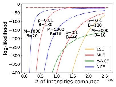
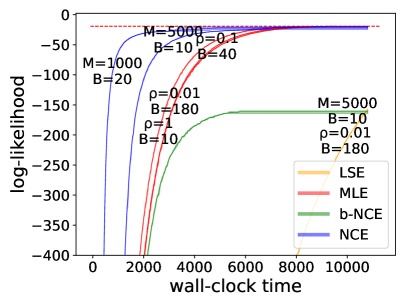
a1 CollegeMsg: neural $q$

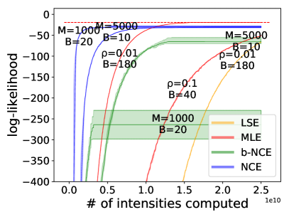
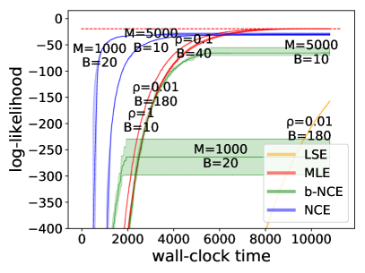
a2 CollegeMsg: Poisson $q$

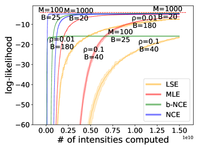
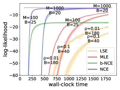
b1 WikiTalk: neural $q$

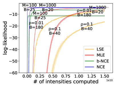
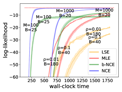
b2 WikiTalk: Poisson $q$

Figure 4: Learning curves of MLE and NCE on the other real-world social interaction datasets.

D.4 Ablation Study I: Always or Never Redraw Noise samples

In Figure 5, we show the learning curves for the “always redraw” and “never redraw” strategies on the first synthetic dataset. As shown in Figure 5(a), with the “always redraw” strategy, NCE ( ) needs considerably fewer intensity evaluations to reach the highest log-likelihood ( ) that MLE ( ) can achieve on the held-out data. However, the curve with $M=1000$ increases more slowly than MLE in terms of wall-clock time since it spends too much time on drawing new noise samples.

As shown in Figure 5(b), with the “never redraw” strategy, $M=1000$ overtakes MLE: a single draw of $M=1000$ noise streams is able to give very good training signals and the saved computation can be spent on training $p_{\theta}$ repeatedly on the same samples. However, the curve of $M=1$ only achieves $\text{log-likelihood}\approx-200$ and thus falls out of the zoomed-in view.

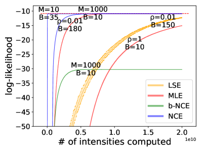
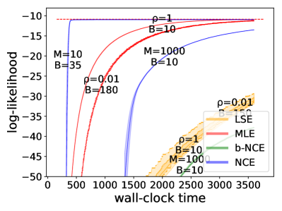
(a) Always redraw new noise samples

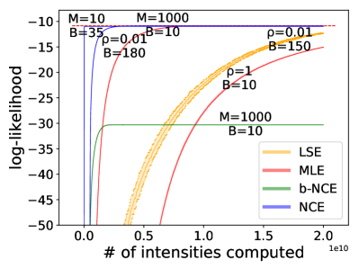
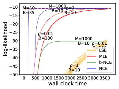
(b) Never redraw new noise samples

Figure 5: Ablation Study I. Learning curves of MLE and NCE with $q=p^{*}$ and different “redraw” strategies.

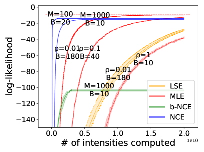
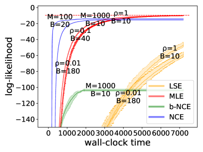
(a) EuroEmail

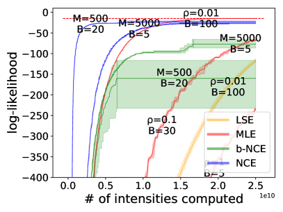
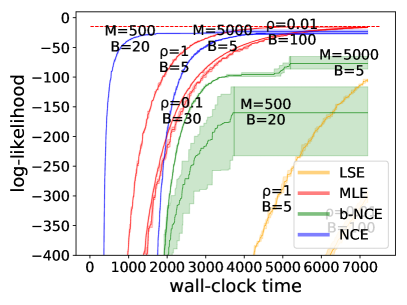
(b) BitcoinOTC

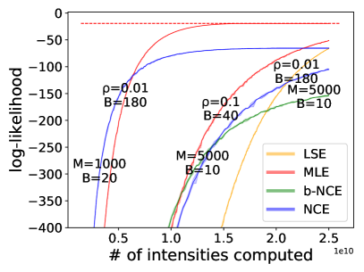
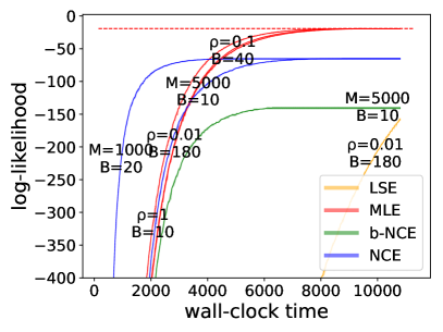
(c) CollegeMsg

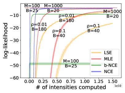
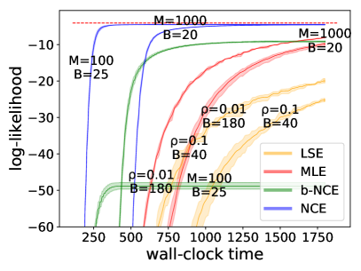
(d) WikiTalk

Figure 6: Ablation Study II. Learning curves of MLE and NCE with untrained $q$ on social interaction datasets.

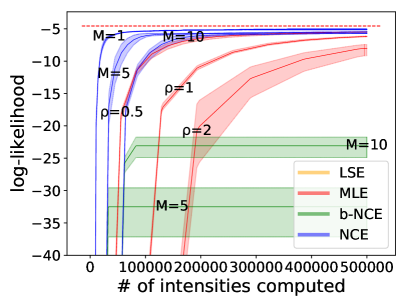
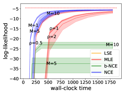
(a) RoboCup

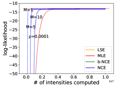
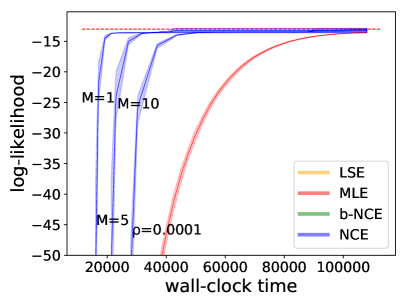
(b) IPTV

Figure 7: Ablation Study III. Learning curves of MLE and NCE using neural $q$ with $C=1$.

D.5 Ablation Study II: NCE with Untrained Noise Distribution

In Figure 6, we show the learning curves of NCE with untrained noise distributions on the real-world social interaction datasets. As we can see, NCE in this setting tends to end up with worse generalization (interestingly except on WikiTalk) and suffers slow convergence (on BitcoinOTC and CollegeMsg) and large variance (on BitcoinOTC).

D.6 Ablation Study III: Effect of $C$

In Figure 7, we show learning curves of NCE using the neural $q$ with $C=1$. Taking $C=1$ means that the same number of noise samples can be drawn faster (with fewer intensity evaluations). However, more training epochs may be needed because the noise looks less like true observations and so NCE’s discrimination tasks are less challenging (see endnote 7).

On the RoboCup dataset, $C=1$ exhibits similar learning speed to $C=5$ but has slightly worse generalization. On the IPTV dataset, $C=1$ gives a considerable speedup over $C=49$ without harming the final generalization. The NCE curves for $M=5$ and $M=10$ shift substantially to the left, since $C=1$ requires many fewer intensity evaluations.

References

- Baran et al. (2008) Baran, I., Demaine, E. D., and Katz, D. A. Optimally adaptive integration of univariate Lipschitz functions. Algorithmica, 2008.
- Chen & Mooney (2008) Chen, D. L. and Mooney, R. J. Learning to sportscast: A test of grounded language acquisition. In Proceedings of the International Conference on Machine Learning (ICML), 2008.
- Daley & Vere-Jones (2007) Daley, D. J. and Vere-Jones, D. An Introduction to the Theory of Point Processes, Volume II: General Theory and Structure. Springer, 2007.
- Du et al. (2016) Du, N., Dai, H., Trivedi, R., Upadhyay, U., Gomez-Rodriguez, M., and Song, L. Recurrent marked temporal point processes: Embedding event history to vector. In Proceedings of the 22nd ACM SIGKDD International Conference on Knowledge Discovery and Data Mining, 2016.
- Eichler et al. (2017) Eichler, M., Dahlhaus, R., and Dueck, J. Graphical modeling for multivariate Hawkes processes with nonparametric link functions. Journal of Time Series Analysis, 38(2):225–242, March 2017.
- Ferguson (1996) Ferguson, T. S. A Course in Large Sample Theory. Chapman and Hall, 1996.
- Goodfellow et al. (2014) Goodfellow, I., Pouget-Abadie, J., Mirza, M., Xu, B., Warde-Farley, D., Ozair, S., Courville, A., and Bengio, Y. Generative adversarial nets. In Advances in Neural Information Processing Systems (NeurIPS), 2014.
- Guo et al. (2018) Guo, R., Li, J., and Liu, H. INITIATOR: Noise-contrastive estimation for marked temporal point process. In Proceedings of the International Joint Conference on Artificial Intelligence (IJCAI), 2018.
- Gutmann & Hyvärinen (2010) Gutmann, M. and Hyvärinen, A. Noise-contrastive estimation: A new estimation principle for unnormalized statistical models. In Proceedings of the International Conference on Artificial Intelligence and Statistics (AISTATS), 2010.
- Gutmann & Hyvärinen (2012) Gutmann, M. U. and Hyvärinen, A. Noise-contrastive estimation of unnormalized statistical models, with applications to natural image statistics. Journal of Machine Learning Research, 2012.
- Hawkes (1971) Hawkes, A. G. Spectra of some self-exciting and mutually exciting point processes. Biometrika, 1971.
- Jozefowicz et al. (2016) Jozefowicz, R., Vinyals, O., Schuster, M., Shazeer, N., and Wu, Y. Exploring the limits of language modeling. arXiv preprint arXiv:1602.02410, 2016.
- Kingma & Ba (2015) Kingma, D. and Ba, J. Adam: A method for stochastic optimization. In Proceedings of the International Conference on Learning Representations (ICLR), 2015.
- Kumar et al. (2016) Kumar, S., Spezzano, F., Subrahmanian, V., and Faloutsos, C. Edge weight prediction in weighted signed networks. In Proceedings of the International Conference on Data Mining (ICDM), 2016.
- Leskovec et al. (2010) Leskovec, J., Huttenlocher, D., and Kleinberg, J. Governance in social media: A case study of the Wikipedia promotion process. In Proceedings of the International Conference on Web and Social Media (ICWSM), 2010.
- Lewis & Shedler (1979) Lewis, P. A. and Shedler, G. S. Simulation of nonhomogeneous Poisson processes by thinning. Naval Research Logistics Quarterly, 1979.
- Liniger (2009) Liniger, T. J. Multivariate Hawkes processes. PhD thesis, Eidgenössische Technische Hochschule ETH Zürich, Nr. 18403, 2009.
- Ma & Collins (2018) Ma, Z. and Collins, M. Noise-contrastive estimation and negative sampling for conditional models: Consistency and statistical efficiency. In Proceedings of the Conference on Empirical Methods in Natural Language Processing (EMNLP), 2018.
- Mei & Eisner (2017) Mei, H. and Eisner, J. The neural Hawkes process: A neurally self-modulating multivariate point process. In Advances in Neural Information Processing Systems (NeurIPS), 2017.
- Mei et al. (2020) Mei, H., Qin, G., Xu, M., and Eisner, J. Neural Datalog through time: Informed temporal modeling via logical specification. In Proceedings of the International Conference on Machine Learning (ICML), 2020.
- Mikolov et al. (2013) Mikolov, T., Sutskever, I., Chen, K., Corrado, G. S., and Dean, J. Distributed representations of words and phrases and their compositionality. In Advances in Neural Information Processing Systems (NeurIPS), 2013.
- Mnih & Hinton (2009) Mnih, A. and Hinton, G. E. A scalable hierarchical distributed language model. In Advances in Neural Information Processing Systems (NeurIPS), 2009.
- Mnih & Teh (2012) Mnih, A. and Teh, Y. W. A fast and simple algorithm for training neural probabilistic language models. In Proceedings of the International Conference on Machine Learning (ICML), 2012.
- Panzarasa et al. (2009) Panzarasa, P., Opsahl, T., and Carley, K. M. Patterns and dynamics of users’ behavior and interaction: Network analysis of an online community. Journal of the American Society for Information Science and Technology, 2009.
- Paranjape et al. (2017) Paranjape, A., Benson, A. R., and Leskovec, J. Motifs in temporal networks. In Proceedings of the International Conference on Web Search and Data Mining (WSDM), 2017.
- Paszke et al. (2017) Paszke, A., Gross, S., Chintala, S., Chanan, G., Yang, E., DeVito, Z., Lin, Z., Desmaison, A., Antiga, L., and Lerer, A. Automatic differentiation in PyTorch. In Autodiff Workshop at NeurIPS 2017, 2017.
- Vaswani et al. (2013) Vaswani, A., Zhao, Y., Fossum, V., and Chiang, D. Decoding with large-scale neural language models improves translation. In Proceedings of the Conference on Empirical Methods in Natural Language Processing (EMNLP), 2013.
- Xu et al. (2018) Xu, H., Luo, D., and Carin, L. Online continuous-time tensor factorization based on pairwise interactive point processes. In Proceedings of the International Joint Conference on Artificial Intelligence (IJCAI), 2018.