Semi-supervised Autoencoding Projective Dependency Parsing

Abstract

We describe two end-to-end autoencoding models for semi-supervised graph-based projective dependency parsing. The first model is a Locally Autoencoding Parser (LAP) encoding the input using continuous latent variables in a sequential manner; The second model is a Globally Autoencoding Parser (GAP) encoding the input into dependency trees as latent variables, with exact inference. Both models consist of two parts: an encoder enhanced by deep neural networks (DNN) that can utilize the contextual information to encode the input into latent variables, and a decoder which is a generative model able to reconstruct the input. Both LAP and GAP admit a unified structure with different loss functions for labeled and unlabeled data with shared parameters. We conducted experiments on WSJ and UD dependency parsing data sets, showing that our models can exploit the unlabeled data to improve the performance given a limited amount of labeled data, and outperform a previously proposed semi-supervised model.

1 Introduction

Dependency parsing captures bi-lexical relationships by constructing directional arcs between words, defining a head-modifier syntactic structure for sentences, as shown in Figure 1. Dependency trees are fundamental for many downstream tasks such as semantic parsing (Reddy et al., 2016; Marcheggiani and Titov, 2017), machine translation (Bastings et al., 2017; Ding and Palmer, 2007), information extraction (Culotta and Sorensen, 2004; Liu et al., 2015) and question answering (Cui et al., 2005). As a result, efficient parsers (Kiperwasser and Goldberg, 2016; Dozat and Manning, 2017; Dozat et al., 2017; Ma et al., 2018) have been developed using various neural architectures.

[column sep=.15cm, row sep=.1ex, font=] PRP$ & NN & RB &[.45cm] VBZ &[.15cm] VBG & NN & PUNC
My & dog & also & likes & eating & sausage & .
4root 21poss 42nsubj 43advmod 45xcomp 56dobj 47pu

Figure 1: A dependency tree: directional arcs represent head-modifier relation between words.

Despite the success of supervised approaches, they require large amounts of labeled data, particularly when neural architectures are used. Syntactic annotation is notoriously difficult and requires specialized linguistic expertise, posing a serious challenge for low-resource languages. Semi-supervised parsing aims to alleviate this problem by combining a small amount of labeled data and a large amount of unlabeled data, to improve parsing performance over labeled data alone. Traditional semi-supervised parsers use unlabeled data to generate additional features, assisting the learning process (Koo et al., 2008), together with different variants of self-training (Søgaard, 2010). However, these are usually pipe-lined and error-propagation may occur.

In this paper, we propose two end-to-end semi-supervised parsers, illustrated in Figure 2(b), namely Locally Autoencoding Parser (LAP) and Globally Autoencoding Parser (GAP). In LAP, the autoencoder model uses unlabeled examples to learn continuous latent variables of the sentence, which are then used to support tree inference by providing an enriched representation. Unlike LAP which does not perform tree inference when learning from unlabeled examples, in GAP, the dependency trees corresponding to the input sentences are treated as latent variables, and as a result the information learned from unlabeled data aligns better with the final tree prediction task.

Unfortunately, regarding trees as latent variables may cause the computation to be intractable, as the number of possible dependency trees to enumerate is exponentially large. A recent work (Corro and Titov, 2018), dealt with this difficulty by regenerating a particular tree of high possibility through sampling. In this study, we suggest a tractable algorithm for GAP, to directly compute all the possible dependency trees in an arc-decomposed manner, providing a tighter bound compared to (Corro and Titov, 2018)’s with lower time complexity. We demonstrate these advantages empirically by evaluating our model on two dependency parsing data sets. We summarize our contributions as follows:

1. We proposed two autoencoding parsers for semi-supervised dependency parsing, with complementary strengths, trading off speed vs. accuracy;

2. We propose a tractable inference algorithm to compute the expectation of the latent dependency tree analytically for GAP, which is naturally extendable to other tree-structured graphical models;

3. We show improved performance of both LAP and GAP with unlabeled data on WSJ and UD data sets over using labeled data alone, and over a recent semi-supervised parser (Corro and Titov, 2018).

2 Related Work

Most dependency parsing studies fall into two major groups: graph-based and transition-based (Kubler et al., 2009). Graph-based parsers (McDonald, 2006) regard parsing as a structured prediction problem to find the most probable tree, while transition-based parsers (Nivre, 2004, 2008) treat parsing as a sequence of actions at different stages leading to a complete dependency tree.

While earlier works relied on manual feature engineering, in recent years the hand-crafted features were replaced by embeddings and deep neural network architectures that were used to learn representation for scoring structural decisions, leading to improved performance in both graph-based and transition-based parsing (Nivre, 2014; Pei et al., 2015; Chen and Manning, 2014; Dyer et al., 2015; Weiss et al., 2015; Andor et al., 2016; Kiperwasser and Goldberg, 2016; Wiseman and Rush, 2016).

The annotation difficulty for this task, has also motivated work on unsupervised (grammar induction) and semi-supervised approaches to parsing (Tu and Honavar, 2012; Jiang et al., 2016; Koo et al., 2008; Li et al., 2014; Kiperwasser and Goldberg, 2015; Cai et al., 2017; Corro and Titov, 2018). It also leads to advances in using unlabeled data for constituent grammar (Shen et al., 2018b, a)

Similar to other structured prediction tasks, directly optimizing the objective is difficult when the underlying probabilistic model requires marginalizing over the dependency trees. Variational approaches have been widely applied to alleviating this problem, as they try to improve the lower bound of the original objective, and were employed in several recent NLP works (Stratos, 2019; Chen et al., 2018; Kim et al., 2019b, a). Variational Autoencoder (VAE) (Kingma and Welling, 2014) is particularly useful for latent representation learning, and is studied in semi-supervised context as the Conditional VAE (CVAE) (Sohn et al., 2015). Note our work differs from VAE as VAE is designed for tabular data but not for structured prediction, as in our circumstance, the input are the sentential tokens and the output is the dependency tree.

The work mostly related to ours is Corro and Titov (2018)’s as they consider the dependency tree as the latent variable, but their work takes a second approximation to the variational lower bound by an extra step to sample from the latent dependency tree, without identifying a tractable inference. We show that with the given structure, exact inference on the lower bound is achievable without approximation by sampling, which tightens the lower bound.

3 Graph-based Dependency Parsing

A dependency graph of a sentence can be regarded as a directed tree spanning all the words of the sentence, including a special “word”–the ROOT–to originate out. Assuming a sentence of length $l$, a dependency tree can be denoted as $\mathcal{T}=(<h_{0},m_{0}>,<h_{1},m_{1}>,\dots,<h_{l-1},m_{l-1}>),$ where $h_{t}$ is the index in the sequence of the head word of the dependency connecting the $t$th word $m_{t}$ as a modifier.

Our graph-based parsers are constructed by following the standard structured prediction paradigm (McDonald et al., 2005; Taskar et al., 2005). In inference, based on the parameterized scoring function $\mathcal{S}_{\bm{\Lambda}}$ with parameter $\bm{\Lambda}$, the parsing problem is formulated as finding the most probable directed spanning tree for a given sentence $\bm{x}$:

$$\mathcal{T}^{*}=\arg\max_{\tilde{\mathcal{T}}\in\mathbb{T}}\mathcal{S}_{\bm{\Lambda}}(\bm{x},\tilde{\mathcal{T}}),$$

where $\mathcal{T}^{*}$ is the highest scoring parse tree and $\mathbb{T}$ is the set of all valid trees for the sentence $\bm{x}$.

It is common to factorize the score of the entire graph into the summation of its substructures: the individual arc scores (McDonald et al., 2005):

$$\mathcal{S}_{\bm{\Lambda}}(\bm{x},\tilde{\mathcal{T}})=\sum_{(h,m)\in\tilde{\mathcal{T}}}s_{\bm{\Lambda}}(h,m)=\sum_{t=0}^{l-1}s_{\bm{\Lambda}}(h_{t},m_{t}),$$

where $\tilde{\mathcal{T}}$ represents the candidate parse tree, and $s_{\bm{\Lambda}}$ is a function scoring individual arcs. $s_{\bm{\Lambda}}(h,m)$ describes the likelihood of an arc from the head $h$ to its modifier $m$ in the tree. Throughout this paper, the scoring is based on individual arcs, as we focus on first order parsing.

3.1 Scoring Function Using Neural Architecture

We used the same neural architecture as that in Kiperwasser and Goldberg (2016)’s study. We first use a bi-LSTM model to take as input $\bm{u}_{t}=[\bm{p}_{t};\bm{e}_{t}]$ at position $t$ to incorporate contextual information, by feeding the word embedding $\bm{e}_{t}$ concatenated with the POS (part of speech) tag embeddings $\bm{p}_{t}$ of each word. The bi-LSTM then projects $\bm{u}_{t}$ as $\bm{o}_{t}$.

Subsequently a nonlinear transformation is applied on these projections. Suppose the hidden states generated by the bi-LSTM are $[\bm{o}_{0},\bm{o}_{1},\bm{o}_{2},\dots,\bm{o}_{t},\dots,\bm{o}_{l-1}]$, for a sentence of length $l$, we compute the arc scores by introducing parameters $\bm{W}_{h}$, $\bm{W}_{m}$, $\bm{w}$ and $\bm{b}$, and transform them as follows:

$$\bm{r}_{t}^{h-arc} =\bm{W}_{h}\bm{o}_{t};\quad\bm{r}_{t}^{m-arc}=\bm{W}_{m}\bm{o}_{t},$$

$$s_{\bm{\Lambda}}(h,m) =\bm{w}^{\intercal}(\tanh(\bm{r}_{h}^{h-arc}+\bm{r}_{m}^{m-arc}+\bm{b})).$$

In this formulation, we first use two parameters to extract two different representations that carry two different types of information: a head seeking for its modifier (h-arc); as well as a modifier seeking for its head (m-arc). Then a nonlinear function maps them to an arc score.

For a single sentence, we can form a scoring matrix as shown in Figure 3, by filling each entry in the matrix using the score we obtained. Therefore, the scoring matrix is used to represent the head-modifier arc score for all the possible arcs connecting two tokens in a sentence (Zheng, 2017).

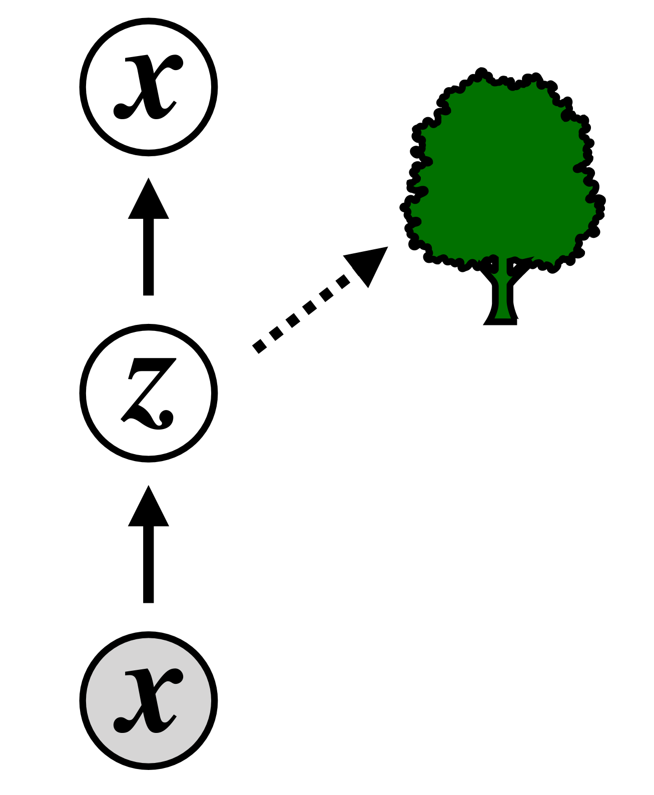
(a) LAP

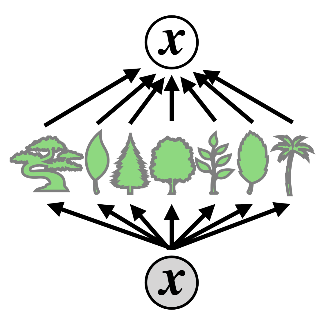
(b) GAP

Figure 2: figure

Illustration of two different parsers. (a) LAP uses continuous latent variable to form the dependency tree (b) GAP treats the dependency tree as the latent variable.

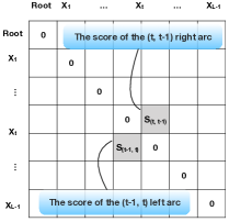
Figure 3: In this illustration of the arc scoring matrix, each entry represents the $(h(head)\rightarrow m(modifier))$ score.

Using the scoring arc matrix, we build graph-based parsers. Since exploring neural architectures for scoring is not our focus, we did not try other complicates, however performance shall be further improved by using advanced neural architectures (Dozat and Manning, 2017; Dozat et al., 2017).

4 Preliminaries

To explain the LAP and GAP models, we briefly review Variational Autoencoders (VAE) and tree CRFs.

Variational Autoencoder (VAE)

The typical VAE is a directed graphical model with Gaussian latent variables, denoted by $\bm{z}$. A generative process first generates latent variable $\bm{z}$ from the prior distribution $\pi(\bm{z})$ and the data $\bm{x}$ is recovered from the distribution $P_{\theta}(\bm{x}|\bm{z})$, parameterized by $\theta$. There is also an inference model $Q(\bm{z}|\bm{x})$, which is an auxiliary posterior distribution, used for inferring the most probable latent variable $\bm{z}$ given the input $\bm{x}$. In our scenario, $\bm{x}$ is an input sequence and $\bm{z}$ is a sequence of latent variables corresponding to it.

The VAE framework seeks to maximize the complete log-likelihood $\log P(\bm{x})$ by marginalizing out the latent variable $\bm{z}$. Since direct parameter estimation of $\log P(\bm{x})$ is usually intractable, a common solution is to maximize its Evidence Lower Bound (ELBO).

Tree Conditional Random Field

Linear chain CRF models an input sequence $\bm{x}=(x_{1}\dots x_{l})$ of length $l$ with labels $\bm{y}=(y_{1}\dots y_{l})$ with globally normalized probability

$$P(\bm{y}|\bm{x})=\frac{\exp{\mathcal{S}(\bm{x},\bm{y})}}{\sum_{\tilde{\bm{y}}\in\mathcal{Y}}\exp{\mathcal{S}(\bm{x},\tilde{\bm{y}})}},$$

where $\mathcal{Y}$ is the set of all the possible label sequences, and $\mathcal{S}(\bm{x},\bm{y})$ the scoring function, usually decomposed as emission ($\sum_{i=1}^{l}s(x_{i},y_{i})$) and transition ($\sum_{i=1}^{l}s(y_{i},y_{i+1})$) for first order models.

Tree CRF models generalize linear chain CRF to trees. For dependency trees, if POS tags are given, the tree CRF model tries to resolve which node pairs should be connected with directed edges, such that the set of edges form a tree. The potentials in the dependency tree take an exponential form, thus the conditional probability of a parse tree $\mathcal{T}$, given the sequence, can be denoted as:

$$P(\mathcal{T}|\bm{x})=\dfrac{\exp{\mathcal{S}(\bm{x},\mathcal{T})}}{Z(\bm{x})},$$ (1)

where $Z(\bm{x})=\sum_{\tilde{\mathcal{T}}\in\mathbb{T}(\bm{x})}\exp{\mathcal{S}(\bm{x},\mathcal{T})}$ is the partition function that sums over all possible valid dependency trees in the set $\mathbb{T}(\bm{x})$ of the given sentence $\bm{x}$.

5 Locally Autoencoding Parser (LAP)

LAP is a fast, semi-supervised parser able to make use of unlabeled data in addition to labeled data. The illustration of this model is displayed in Figure 2(a). LAP learns, using both labeled and unlabeled data, a continuous latent variables representation, designed to support the parsing task by creating contextualized token-representations that capture properties of the full sentence. Typically, each token in the sentence is represented by its latent variable $z_{t}$, which is a high-dimensional Gaussian variable. This configuration ensures the continuous latent variable retains the contextual information from lower-level neural models to assist finding its head or its modifier; as well as forcing the representation of similar tokens closer.

We adjust the original VAE setup in our semi-supervised task by considering examples with labels, similar to recent conditional variational formulations (Sohn et al., 2015; Miao and Blunsom, 2016; Zhou and Neubig, 2017). We propose a full probabilistic model for a given sentence $\bm{x}$, with the unified objective to maximize for both supervised and unsupervised parsing as follows:

$$\mathcal{J}=\log{P_{\bm{\theta}}(\bm{x})P_{\bm{\omega}}^{\epsilon}(\mathcal{T}|\bm{x})},\quad\epsilon=\begin{cases}1,&\text{if}\quad\mathcal{T}\quad\text{exists},\\ 0,&\text{otherwise}.\end{cases}$$

This objective can be interpreted as follows: if the training example has a golden tree $\mathcal{T}$ with it, then the objective is the log joint probability $P_{\bm{\theta},\bm{\omega}}(\mathcal{T},\bm{x})$; if the golden tree is missing, then the objective is the log marginal probability $P_{\bm{\theta}}(\bm{x})$. The probability of a certain tree is modeled by a tree-CRF in Eq. 1 with parameters $\bm{\omega}$ as $P_{\bm{\omega}}(\mathcal{T}|\bm{x})$. Given the assumed generative process $P_{\theta}(\bm{x}|\bm{z})$, directly optimizing this objective is intractable, therefore we instead optimize its Evidence Lower BOund (ELBO) :

$$\mathcal{J}_{lap}= \mathop{\mathbb{E}}\limits_{\bm{z}\sim Q_{\bm{\phi}}(\bm{z}|\bm{x})}\left[\log P_{\bm{\theta}}(\bm{x}|\bm{z})\right]-\mathbb{KL}(Q_{\bm{\phi}}(\bm{z}|\bm{x})||P_{\bm{\theta}}(\bm{z}))$$

$$+\epsilon\mathop{\mathbb{E}}\limits_{\bm{z}\sim Q_{\bm{\phi}}(\bm{z}|\bm{x})}\left[\log P_{\bm{\omega}}(\mathcal{T}|\bm{z})\right].$$

We show $J_{lap}$ is the ELBO of $J$ in the appendix A.1. In practice, similar as VAE-style models, $\mathop{\mathbb{E}}\limits_{\bm{z}\sim Q_{\bm{\phi}}(\bm{z}|\bm{x})}\left[\log P_{\bm{\theta}}(\bm{x}|\bm{z})\right]$ is approximated by $\frac{1}{N}\sum_{j=1}^{N}\log P_{\bm{\theta}}(\bm{x}|\bm{z}_{j})$ and $\mathop{\mathbb{E}}\limits_{\bm{z}\sim Q_{\bm{\phi}}(\bm{z}|\bm{x})}\left[\log P_{\bm{\omega}}(\mathcal{T}|\bm{z})\right]$ by $\frac{1}{N}\sum_{j=1}^{N}\log P_{\bm{\omega}}(\mathcal{T}|\bm{z}_{j})$, where $\bm{z}_{j}$ is the $j$-th sample of $N$ samples sampled from $Q_{\bm{\phi}}(\bm{z}|\bm{x})$. At prediction stage, we simply use $\mu_{\bm{z}}$ rather than sampling $\bm{z}$. During the inference stage, the tree-Viterbi algorithm ensures the output is a projective dependency tree.

6 Globally Autoencoding Parser (GAP)

LAP autoencodes the input locally at the sequence level, focusing on the textual representation in isolation by connecting them to the parsing algorithm. A better approach is to treat the entire dependency tree as a structured latent variable to reconstruct the input.

We design a different model, GAP, by building a model containing both a discriminative component and a generative component to jointly learn the downstream representations and the dependency structure construction. The discriminative component builds a neural CRF model for dependency tree construction, and the generative model reconstructs the sentence from the factor graph as a Bayesian network, by assuming a generative process in which each head generates its modifier. Concretely, the latent variable in this model is the dependency tree structure.

6.1 Discriminative Component: the Encoder

We model the discriminative component in our model as $P_{\bm{\Phi}}(\mathcal{T}|\bm{x})$ parameterized by $\bm{\Phi}$, taking the same form as in Eq. 1. Typically in our model, $\bm{\Phi}$ are the parameters of the underlying neural networks, whose architecture is described in Sec. 3.1.

6.2 Generative Component: the Decoder

We use a set of conditional categorical distributions to construct our Bayesian network decoder. More specifically, using the head $h$ and modifier $m$ notation, each head reconstructs its modifier with the probability $P(m_{t}|h_{t})$ for the $t$th word in the sentence ($0$th word is always the special “ROOT” word), which is parameterized by the set of parameters $\bm{\Theta}$. Given $\bm{\Theta}$ as a matrix of $|\mathcal{V}|$ by $|\mathcal{V}|$, where $|\mathcal{V}|$ is the vocabulary size, $\theta_{mh}$ is the item on row $m$ column $h$ denoting the probability that the head word $h$ generates $m$. In addition, we have a simplex constraint $\sum_{m\in\mathcal{V}}\theta_{mh}=1$. The probability of reconstructing the input $\bm{x}$ as modifiers $\bm{m}$ in the generative process is

$$P_{\bm{\Theta}}(\bm{m}|\mathcal{T})=\prod_{t=0}^{l-1}P(m_{t}|h_{t})=\prod_{t=0}^{l-1}\theta_{m_{t}h_{t}},$$

where $l$ is the sentence length and $P(m_{t}|h_{t})$ represents the probability a head generating its modifier.

6.3 A Unified Supervised and Unsupervised Learning Framework

With the design of the discriminative component and the generative component of the proposed model, we have a unified learning framework for sentences with or without golden parse tree.

The complete data likelihood of a given sentence, if the golden tree is given, is

$$P_{\bm{\Theta},\bm{\Phi}}(\bm{m},\mathcal{T}|\bm{x})= P_{\bm{\Theta}}(\bm{m}|\mathcal{T})P_{\bm{\Phi}}(\mathcal{T}|\bm{x})$$

$$= \left[\prod_{t=1}^{l}P(m_{t}|h_{t})\right]\dfrac{\exp{\mathcal{S}_{\bm{\Phi}}(\bm{x},\mathcal{T})}}{Z(\bm{x})}$$

$$= \dfrac{\exp{\sum\limits_{(h,m)\in\mathcal{T}}s^{{}^{\prime}}_{\bm{\Phi},\bm{\Theta}}(h,m)}}{Z(\bm{x})},$$

where $s^{{}^{\prime}}_{\bm{\Phi},\bm{\Theta}}(h,m)=s_{\bm{\Phi}}(h,m)+\log\theta_{mh}$, with $\bm{m},\bm{x}$ and $\mathcal{T}$ all observable.

For a unlabeled sentence, the complete data likelihood can be obtained by marginalizing over all the possible parse trees in the set $\mathbb{T}(\bm{x})$:

$$P_{\bm{\Theta},\bm{\Phi}}(\bm{m}|\bm{x})= \sum_{\mathcal{T}\in\mathbb{T}(\bm{x})}P_{\bm{\Theta},\bm{\Phi}}(\bm{m},\mathcal{T}|\bm{x})$$

$$= \dfrac{U(\bm{x})}{Z(\bm{x})},$$

where $U(\bm{x})=\sum_{\mathcal{T}\in\mathbb{T}(\bm{x})}\exp{\sum\limits_{(h,m)\in\mathcal{T}}s^{{}^{\prime}}_{\bm{\Phi},\bm{\Theta}}(h,m)}$.

We adapted a variant of Eisner (1996)’s algorithm to marginalize over all possible trees to compute both $Z$ and $U$, as $U$ has the same structure as $Z$, assuming a projective tree. This algorithm also enforces the output is a projective dependency tree.

We use log-likelihood as our objective function. The objective for a sentence with golden tree is:

$$\mathcal{J}_{l}= \log P_{\bm{\Theta},\bm{\Phi}}(\bm{m},\mathcal{T}|\bm{x})$$

$$= \sum\limits_{(h,m)\in\mathcal{T}}s^{{}^{\prime}}_{\bm{\Phi},\bm{\Theta}}(h,m)-\log Z(\bm{x})$$

If the input sentence does not have an annotated golden tree, then the objective is:

$$\mathcal{J}_{u}= \log P_{\bm{\Theta},\bm{\Phi}}(\bm{m}|\bm{x})$$

$$= \log U(\bm{x})-\log Z(\bm{x}).$$ (2)

Thus, during training, the objective function with shared parameters is chosen based on whether the sentence in the corpus has golden parse tree or not.

6.4 Learning

Directly optimizing the loss in Eq.2 is difficult when using the unlabeled data, and may lead to undesirable shallow local optima. Instead, we derive the evidence lower bound (ELBO) of $\log P_{\bm{\Theta},\bm{\Phi}}(\bm{m}|\bm{x})$ as follows, by denoting $Q(\mathcal{T})=P_{\bm{\Theta},\bm{\Phi}}(\mathcal{T}|\bm{m},\bm{x})$ as the posterior:

$$\log P_{\bm{\Theta},\bm{\Phi}}(\bm{m}|\bm{x}) =\log\sum_{\mathcal{T}}Q(\mathcal{T})\dfrac{P_{\bm{\Theta},\bm{\Phi}}(\bm{m},\mathcal{T}|\bm{x})}{Q(\mathcal{T})}$$

$$=\log\mathbb{E}_{\mathcal{T}\sim Q(\mathcal{T})}\dfrac{P_{\bm{\Theta},\bm{\Phi}}(\bm{m},\mathcal{T}|\bm{x})}{Q(\mathcal{T})}$$

$$\geq\mathbb{E}_{\mathcal{T}\sim Q(\mathcal{T})}\log\dfrac{P_{\bm{\Theta},\bm{\Phi}}(\bm{m},\mathcal{T}|\bm{x})}{Q(\mathcal{T})}$$

$$=\mathbb{E}_{\mathcal{T}\sim Q(\mathcal{T})}\left[\log P_{\bm{\Theta}}(\bm{m}|\mathcal{T})\right]$$

$$-\mathbb{KL}\left[Q(\mathcal{T})||P_{\bm{\Phi}}(\mathcal{T}|\bm{x})\right].$$

Instead of maximizing the log-likelihood directly, we alternatively maximize the ELBO, so our new objective function for unlabeled data becomes

$$\max_{\bm{\Theta},\bm{\Phi}} \mathbb{E}_{\mathcal{T}\sim Q(\mathcal{T})}\left[\log P_{\bm{\Theta}}(\bm{m}|\mathcal{T})\right]-\mathbb{KL}\left[Q(\mathcal{T})||P_{\bm{\Phi}}(\mathcal{T}|\bm{x})\right].$$

Note instead of using sampling to approximate the ELBO above as in Corro and Titov (2018)’s work: $\mathbb{E}_{\mathcal{T}\sim Q(\mathcal{T})}\left[\log P_{\bm{\Theta}}(\bm{m}|\mathcal{T})\right]-\mathbb{KL}\left[Q(\mathcal{T})||P_{\bm{\Phi}}(\mathcal{T}|\bm{x})\right]\approx\frac{1}{N}\sum_{j=1}^{N}\left[\log P_{\bm{\Theta}}(\bm{m}|\mathcal{T}_{j})\right]-\mathbb{KL}\left[Q(\mathcal{T}_{j})||P_{\bm{\Phi}}(\mathcal{T}_{j}|\bm{x})\right]$, we identify a tractable algorithm to calculate it directly, tightening the bound.

In addition, to account for the unambiguity in the posterior, we incorporate entropy regularization (Tu and Honavar, 2012) when applying our algorithm, by adding an entropy term $-\sum_{\mathcal{T}}Q(\mathcal{T})\log Q(\mathcal{T})$ with a non-negative factor $\sigma$ when the input sentence does not have a golden tree. Adding this regularization term is equivalent as raising the expectation of $Q(\mathcal{T})$ to the power of $\frac{1}{1-\sigma}$. We annealed $\sigma$ from the beginning of training to the end, as in the beginning, the generative model is well initialized by sentences with golden trees that resolve disambiguity. The details of training are shown in Alg. 1.

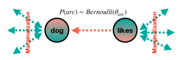
Figure 4: We illustrate the tractable inference procedure by marginalization in a arc-decomposed manner.

Algorithm 1 Learning Algorithm for GAP

1:Initialize the parameter $\bm{\Theta}$ in the decoder with the labeled data set $\{\bm{x},\mathcal{T}\}^{l}$.

2:Initialize $\bm{\Lambda}$ in the encoder randomly.

3:for $t$ in $epochs$ do

4:     for sentence $\bm{x}_{i}^{l}$ with golden parse tree $\mathcal{T}_{i}^{l}$ in the labeled data set $\{\bm{x},\mathcal{T}\}^{l}$ do

5:         Stochastically update the parameter $\bm{\Lambda}$ in the encoder using Adam while fixing the decoder.

6:     end for

7:     Initialize a Counting Buffer $\mathcal{B}$

8:     for unlabeled sentence $\bm{x}_{i}^{u}$ in the unlabeled data set $\{\bm{x}\}^{u}$ do

9:         Compute the posterior $Q(\mathcal{T})$ in an arc factored manner for $\bm{x}_{i}^{u}$ tractably.

10:         Compute the expectation of all possible $(h(head)\rightarrow m(modifier))$ occurrence in the sentence $\bm{x}$ based on $Q(\mathcal{T})$.

11:         Update buffer $\mathcal{B}$ using the expectation to the power for $\frac{1}{1-\sigma}$ of all possible $(h\rightarrow m)$.

12:     end for

13:     Obtain $\bm{\Theta}$ globally and analytically based on the buffer $\mathcal{B}$ and renew the decoder.

14:end for

6.5 Convexity of ELBO w.r.t. $\bm{\Theta}$

In practice, we found the model benefits more by fixing the parameter $\bm{\Phi}$ when the data is unlabeled and optimizing the ELBO w.r.t. the parameter $\bm{\Theta}$. We attribute this to the strict convexity of the ELBO w.r.t. $\bm{\Theta}$, by sketching the proof in Appendix A.2.

6.6 Tractable Inference

The common approach to approximate the expectation of the latent variables from the posterior distribution $Q(\mathcal{T})$ is via sampling in VAE-type models (Kingma and Welling, 2014). In a significant contrast to that, we argue in this GAP model the expectation of the latent variable (which is the dependency tree structure) is analytically tractable by designing a variant of the inside-outside algorithm (Eisner, 1996; Paskin, 2001) in an arc decomposed manner. This can be done by regarding each directed arc as an indicator variable from a Bernoulli distribution, implying whether the arc exists or not. We argue that assuming the dependency tree is projective, specialized belief propagation algorithm exists to compute not only the marginalization over all other arcs but also the target arc. This algorithm also computes the expectation of each arc analytically, making inference tractable. This idea is illustrated in Figure 4. We show the details of this algorithm in the appendix A.4. We also show how to calculate the expectation w.r.t the posterior distribution $Q(\mathcal{T})$ in appendix A.3.

7 Experiments

7.1 Experimental Settings

Data sets

First we compared our models’ performance with strong baselines on the WSJ data set, which is the Stanford Dependency conversion (De Marneffe and Manning, 2008) of the Penn Treebank (Marcus et al., 1993) using the standard section split: 2-21 for training, 22 for development and 23 for testing. Second we evaluated our models on multiple languages, using data sets from UD (Universal Dependency) 2.3 (Mcdonald et al., 2013). Since semi-supervised learning is particularly useful for low-resource languages, we believe those languages in UD can benefit from our approach. The statistics of the data used in our experiments are described in Table 1.

To simulate the low-resource language environment, we used $10\%$ of the whole training set as the annotated, and the rest $90\%$ as the unlabeled.

Language	WSJ	Dutch	Spanish	English	French	Croatian	German	Italian	Russian	Japanese
Training	39832	12269	14187	2914	14450	6983	13814	13121	3850	7133
Development	1700	718	1400	707	1476	849	799	564	579	511
Testing	2416	596	426	769	416	1057	977	482	601	551

Table 1: Statistics of multiple languages we used in our experiments are shown here. The table shows number of sentences in the training, development and test data divisions.

Model	Dutch	Spanish	English	French	Croation	German	Italian	Russian	Japanese
NMP (L)	76.11	82.00	75.51	83.07	77.44	74.07	82.85	75.18	93.46
NTP (L)	76.20	82.09	75.57	83.12	77.51	74.13	82.99	75.23	93.54
LAP (L)	76.15	81.93	75.36	83.09	77.45	74.14	83.07	74.84	93.38
GAP (L)	76.23	81.97	75.75	83.11	77.49	74.16	83.14	75.17	93.52
CRFAE (L+U)	71.32	74.67	68.52	77.35	69.89	68.44	76.37	68.64	87.26
ST (L+U)	75.37	80.86	72.76	81.38	76.10	73.45	82.74	72.57	91.43
LAP (L+U)	76.29	82.48	75.48	83.23	77.78	74.48	83.34	75.22	93.65
GAP (L+U)	76.54	82.56	76.21	83.26	77.83	74.63	83.54	75.69	93.92

Table 2: In this table we compare different models on multiple languages from UD. Models were trained in a fully supervised fashion with labeled data only (noted as “L”) or semi-supervised (notes as “L+U”). “ST” stands for self-training.

Training

In the training phase, we use Adam (Kingma and Ba, 2014) to update all the parameters in both LAP and GAP, except the parameters in the decoder in GAP, which are updated by using their global optima in each epoch. In GAP, We annealed $\sigma$ from $1$ to $0.3$. We did not take efforts to tune models’ hyper-parameters and they remained the same across all the experiments. To preventing over-fitting, we applied the “early stop” strategy by using the development set.

7.2 Semi-Supervised Dependency Parsing on WSJ Data Set

We first evaluate our models on the WSJ data set and compared the model performance with other semi-supervised parsing models, including CRFAE (Cai et al., 2017), which is originally designed for dependency grammar induction but can be modified for semi-supervised parsing, and “differentiable Perturb-and-Parse” parser (DPPP) (Corro and Titov, 2018). To contextualize the results, we also experiment with the supervised neural margin-based parser (NMP) (Kiperwasser and Goldberg, 2016), neural tree-CRF parser (NTP) and the supervised version of LAP and GAP, with only the labeled data. To ensure a fair comparison, our experimental set up on the WSJ is identical as that in DPPP, using the same 100 dimension skip-gram word embeddings employed in an earlier transition-based system (Dyer et al., 2015). We show our experimental results in Table 3.

Model	UAS
DPPP(Corro and Titov, 2018)(L)	88.79
DPPP(Corro and Titov, 2018)(L+U)	89.50
CRFAE(Cai et al., 2017)(L+U)	82.34
NMP(Kiperwasser and Goldberg, 2016)(L)	89.64
NTP (L)	89.63
Self-training (L+U)	87.81
LAP (L)	89.37
LAP (L+U)	89.49
GAP (L)	89.65
GAP (L+U)	89.96

Table 3: Comparing model performance on WSJ data set with $10\%$ labeled data. “L” means only $10\%$ labeled data is used, while “L+U” means both $10\%$ labeled and $90\%$ unlabeled data are used.

As shown in this table, both of our LAP and GAP model are able to utilize the unlabeled data to increase the overall performance comparing with only using labeled data. Our LAP model performs slightly worse than the NMP model, which we attribute to the increased model complexity by incorporating extra encoder and decoders to deal with the latent variable. However, our LAP model achieved comparable results on semi-supervised parsing as the DPPP model, while our LAP model is simple and straightforward without additional inference procedure. Instead, the DPPP model has to sample from the posterior of the structure by using a “GUMBEL-MAX trick” to approximate the categorical distribution at each step, which is intensively computationally expensive. Further, our GAP model achieved the best results among all these methods, by successfully leveraging the the unlabeled data in an appropriate manner. We owe this success to such a fact: GAP is able to calculate the exact expectation of the arc-decomposed latent variable, the dependency tree structure, in the ELBO for the complete data likelihood when the data is unlabeled, rather than using sampling to approximate the true expectation. Self-training using NMP with both labeled and unlabeled data is also included as a base-line, where the performance is deteriorated without appropriately using the unlabeled data.

7.3 Semi-supervised Dependency Parsing on the UD Data Set

We also evaluated our models on multiple languages from the UD data and compared the performance with the semi-supervised version of CRFAE and the fully supervised NMP and NTP. To fully simulate the low-resource scenario, we did not use any external word embeddings but initializing them randomly.

We summarize the results in Table 2. First, when using labeled data only, LAP and GAP have similar performance as NMP and NTP. Second, we note that our LAP and GAP models do benefit from the unlabeled data, compared to using labeled data only. Both our LAP and GAP model are able to exploit the hidden information in the unlabeled data to improve the performance. Comparing between LAP and GAP, we notice GAP in general has better performance than LAP, and can better leverage the information in the unlabeled data to boost the performance. These results validate that GAP is especially useful for low-resource languages with few annotations. We also experimented using self-training on the labeled and unlabeled data with the NMP model. As results show, self-training deteriorate the performance especially when the size of the training data is small.

8 Comparison of Complexity

We briefly compare the complexity of LAP, GAP and their competitors in Table 4. As can be seen, though all the algorithms are of $O(l^{3})$ complexity, the constant differs significantly. Our LAP model is 6 times faster than the DPPP algorithm while our GAP model is 2 times faster. Considering the model performance, our models are favored.

Model	Complexity (Train)	Complexity (Eval)
DPPP	24$l^{3}$	4$l^{3}$
CRFAE	12$l^{3}$	4$l^{3}$
NMP	4$l^{3}$	4$l^{3}$
NTP	4$l^{3}$	4$l^{3}$
LAP	4$l^{3}$	4$l^{3}$
GAP	12$l^{3}$	4$l^{3}$

Table 4: We compare the complexity of different models, with $l$ indicating the sentence length.

9 Conclusion

In this paper, we present two semi-supervised parsers, namely locally autoencoding parser (LAP) and globally autoencoding parser (GAP). Both are end-to-end learning systems enhanced with neural architectures, capable of utilizing the latent information within the unlabeled data together with labeled data to improve the parsing performance, without using external resources. More importantly, GAP outperforms the previous published (Corro and Titov, 2018) semi-supervised parsing system on the WSJ data set. We attribute this success to two reasons: First, GAP consists both a discriminative component and a generative component, which are constraining and supplementing each other such that final parsing choices are made in a checked-and-balanced manner to avoid over-fitting. Second, instead of sampling from posterior of the latent variable (the dependency tree), GAP analytically computes the expectation and marginalization, hence the decoder’s global optima can be found, leading to improved performance.

10 Acknowledgements

We sincerely appreciate Prof. Kewei Tu for his valuable inspiration, comments, discussion and suggestions. We also thank Ge Wang, Dingquan Wang, Jiong Cai for their constructive discussion. We extend our thanks to all the anonymous reviewers for their insightful feedback. This work was partially funded by an Nvidia GPU grant.

Appendix A Appendix

A.1 ELBO of LAP’s Original Ojective

Given an input sequence $\bm{x}$, we prove that $\mathcal{J}_{lap}$ is the ELBO of $\mathcal{J}$:

Lemma A.1.

$\mathcal{J}_{lap}$ is the ELBO (evidence lower bound) of the original objective $\mathcal{J}$, with an input sequence $\bm{x}$.

Denote the encoder $Q$ is a distribution used to approximate the true posterior distribution $P_{\bm{\phi}}(\bm{z}|\bm{x})$, parameterized by $\bm{\phi}$ such that $Q$ encoding the input into the latent space $\bm{z}$.

Proof.

$$\log{P_{\bm{\theta}}(\bm{x})P_{\bm{\omega}}^{\epsilon}(\mathcal{T}|\bm{x})}= \underbrace{\log{P_{\bm{\theta}}(\bm{x})}}_{\mathcal{U}}+\underbrace{\epsilon\log{P_{\bm{\omega}}(\mathcal{T}|\bm{x})}}_{\mathcal{L}}$$

$$\mathcal{U}= \log\int_{z}Q_{\bm{\phi}}(\bm{z}|\bm{x})\dfrac{P_{\bm{\theta}}(\bm{x})}{Q_{\bm{\phi}}(\bm{z}|\bm{x})}d_{z}$$

$$\geq \mathop{\mathbb{E}}\limits_{\bm{z}\sim Q_{\bm{\phi}}(\bm{z}|\bm{x})}\left[\log P_{\bm{\theta}}(\bm{x}|\bm{z})\right]$$

$$- \mathop{\mathbb{E}}\limits_{\bm{z}\sim Q_{\bm{\phi}}(\bm{z}|\bm{x})}\left[\log\dfrac{Q_{\bm{\phi}}(\bm{z}|\bm{x})}{P_{\bm{\theta}}(\bm{x})}\right]$$

$$= \mathop{\mathbb{E}}\limits_{\bm{z}\sim Q_{\bm{\phi}}(\bm{z}|\bm{x})}\left[\log P_{\bm{\theta}}(\bm{x}|\bm{z})\right]$$

$$- \mathbb{KL}\left(Q_{\bm{\phi}}(\bm{z}|\bm{x})||P_{\bm{\theta}}(\bm{z})\right),$$

(ELBO of traditional VAE)

$$\mathcal{L}= \epsilon\log{P_{\bm{\omega}}(\mathcal{T}|\bm{x})}$$

$$= \epsilon\log{\int_{z}P_{\bm{\omega}}(\mathcal{T}|\bm{z})Q_{\bm{\phi}}(\bm{z}|\bm{x})d_{z}}$$

$$= \epsilon\log{\mathop{\mathbb{E}}\limits_{\bm{z}\sim Q_{\bm{\phi}}(\bm{z}|\bm{x})}\left[P_{\bm{\omega}}(\mathcal{T}|\bm{z})\right]}$$

$$\geq \epsilon\mathop{\mathbb{E}}\limits_{\bm{z}\sim Q_{\bm{\phi}}(\bm{z}|\bm{x})}\left[\log P_{\bm{\omega}}(\mathcal{T}|\bm{z})\right].$$

Combining $\mathcal{U}$ and $\mathcal{L}$ leads to the fact:

$$\mathcal{U}+\mathcal{L}\geq \mathop{\mathbb{E}}\limits_{\bm{z}\sim Q_{\bm{\phi}}(\bm{z}|\bm{x})}\left[\log P_{\bm{\theta}}(\bm{x}|\bm{z})\right]-\mathbb{KL}(Q_{\bm{\phi}}(\bm{z}|\bm{x})||P_{\bm{\theta}}(\bm{z}))$$

$$+ \epsilon\mathop{\mathbb{E}}\limits_{\bm{z}\sim Q_{\bm{\phi}}(\bm{z}|\bm{x})}\left[\log P_{\bm{\omega}}(\mathcal{T}|\bm{z})\right]=\mathcal{J}_{lap}$$

∎

A.2 Convexity of ELBO w.r.t $\bm{\Theta}$ in GAP

Since we only care about the term containing $\bm{\Theta}$, the KL divergence term degenerates to a constant. For sentence $i$, $Q(\mathcal{T}_{i})$ has been derived in the previous section as matrix $\bm{P}$ and $\mathbbm{1}$ is the indication function.

$$\max_{\bm{\Theta}} \sum\limits_{i}\mathbb{E}_{\mathcal{T}_{i}\sim Q(\mathcal{T}_{i})}\left[\log P_{\bm{\Theta}}(\bm{m}_{i}|\mathcal{T}_{i})\right]$$

$$-\mathbb{KL}\left[Q(\mathcal{T}_{i})||P_{\bm{\Phi}}(\mathcal{T}_{i}|\bm{x}_{i})\right]$$

$$\max_{\bm{\Theta}} \sum\limits_{i}\sum\limits_{\mathcal{T}_{i}\in\mathbb{T}(\bm{x_{i}})}Q(\mathcal{T}_{i})\log P_{\bm{\Theta}}(\bm{m}_{i}|\mathcal{T}_{i})+Const$$

$$\max_{\bm{\Theta}} \sum\limits_{(h\rightarrow m)}\log\theta_{mh}\mathrm{E}_{(h\rightarrow m)\sim Q}\mathbbm{1}(h\rightarrow m)$$

$$\max_{\bm{\Theta}} \sum\limits_{(h\rightarrow m)}Q(\mathbbm{1}(h\rightarrow m))\log\theta_{mh},$$ (3)

$$Q(\mathbbm{1}(h\rightarrow m))$$ is a Bernoulli distribution,

indicating whether the arc $$(h\rightarrow m)$$ exists.

$$s.t. \sum\limits_{m}\theta_{mh}=1\quad\forall h.$$ (4)

A.3 Marginalization and Expectation of Latent Parse Trees

Light modification is needed in our study to calculate the expectation w.r.t. the posterior distribution $Q(\mathcal{T})=P_{\bm{\Theta},\bm{\Phi}}(\mathcal{T}|\bm{m},\bm{x})$, as we have

$$P_{\bm{\Theta},\bm{\Phi}}(\mathcal{T}|\bm{m},\bm{x})=\dfrac{P_{\bm{\Theta},\bm{\Phi}}(\mathcal{T},\bm{m}|\bm{x})}{P_{\bm{\Theta},\bm{\Phi}}(\bm{m}|\bm{x})}$$

$$=\dfrac{\exp^{\sum\limits_{(h,m)\in\mathcal{T}}s^{{}^{\prime}}_{\bm{\Phi},\bm{\Theta}}(h,m)}}{Z(\bm{x})}/\sum_{\mathcal{T}\in\mathbb{T}}\left[\dfrac{\exp^{\sum\limits_{(h,m)\in\mathcal{T}}s^{{}^{\prime}}_{\bm{\Phi},\bm{\Theta}}(h,m)}}{Z(\bm{x})}\right]$$

$$=\dfrac{\exp{\sum\limits_{(h,m)\in\mathcal{T}}s^{{}^{\prime}}_{\bm{\Phi},\bm{\Theta}}(h,m)}}{Z^{\prime}(\bm{x})}$$ ,

where $Z^{\prime}(\bm{x})=\sum_{\mathcal{T}\in\mathbb{T}}\exp{\sum\limits_{(h,m)\in\mathcal{T}}s^{{}^{\prime}}_{\bm{\Phi},\bm{\Theta}}(h,m)}$ is the real marginal we need to calculate using the transformed scoring matrix $\bm{S}^{\prime}$ as input in the inside algorithm. Each entry in this transformed scoring matrix is defined in the text as $s^{{}^{\prime}}_{\bm{\Phi},\bm{\Theta}}(h,m)$.

A.4 Algorithm Details for GAP

Assuming the sentence is of length $l$, we could obtain an arc decomposed scoring matrix $\bm{S}$ of size $l\times l$, with the entry $\bm{S}[i,j]_{i\neq j,j\neq 0}$ stands for the arc score where $i$th word is the head and $j$th word the modifier.

We first describe the inside algorithm to compute the marginalization of all possible projective trees in Algo.2.

Algorithm 2 Inside Algorithm

Input: $\bm{S}$
      Output: $\bm{\alpha},Z$

1:$\bm{\alpha}\leftarrow-\infty$

2:for $s\in 0\dots l-1$ do

3:     if $s>0$ then

4:         $\bm{\alpha}[s,s,L,C]\leftarrow 0$

5:     end if

6:     $\bm{\alpha}[s,s,R,C]\leftarrow 0$

7:end for

8:for $k\in 1\dots l-1$ do

9:     for $s\in 0\dots l-k$ do

10:         $t=s+k$

11:         if $s>0$ then

12:              $\bm{\alpha}[s,t,L,I]\leftarrow\log\sum\limits_{u\in[s,t-1]}\exp\left(\bm{\alpha}[s,u,R,C]+\bm{\alpha}[u+1,t,L,C]\right)+\bm{S}[t,s]$

13:              

14:         end if

15:         $\bm{\alpha}[s,t,R,I]\leftarrow\log\sum\limits_{u\in[s,t-1]}\exp\left(\bm{\alpha}[s,u,R,C]+\bm{\alpha}[u+1,t,L,C]\right)+\bm{S}[s,t]$

16:         

17:         if $s>0$ then

18:              $\bm{\alpha}[s,t,L,C]\leftarrow\log\sum\limits_{u\in[s,t-1]}\exp\left(\bm{\alpha}[s,u,L,C]+\bm{\alpha}[u,t,L,I]\right)$

19:              

20:         end if

21:         $\bm{\alpha}[s,t,R,C]\leftarrow\log\sum\limits_{u\in[s,t-1]}\exp\left(\bm{\alpha}[s,u+1,R,I]+\bm{\alpha}[u+1,t,R,C]\right)$

22:         

23:     end for

24:end for

25:$Z\leftarrow\bm{\alpha}[0,l-1,R,C]$

We then describe the outside algorithm to compute the outside tables in Algo. 3. In this algorithm, $\bigoplus$ stands for the logaddexp operation.

Algorithm 3 Outside Algorithm

Input: $\bm{S},\bm{\alpha}$
      Output: $\bm{\beta}$

1:$\bm{\beta}\leftarrow-\infty$

2:$\bm{\beta}[0,l-1,R,C]\leftarrow 0$

3:for $k\in l-1\dots 1$ do

4:     for $s\in 0\dots l-k$ do

5:         $t=s+k$

6:         for $u\in s\dots t-1$ do

7:              $\bm{\beta}[s,u+1,R,I]\leftarrow\bigoplus(\bm{\beta}[s,u+1,R,I],\bm{\beta}[s,t,R,C]+\bm{\alpha}[u+1,t,R,C])$

8:              

9:         end for

10:         for $u\in s\dots t-1$ do

11:              $\bm{\beta}[u+1,t,R,C]\leftarrow\bigoplus(\bm{\beta}[u+1,t,R,C],\bm{\beta}[s,t,R,C]+\bm{\alpha}[s,u+1,R,I])$

12:              

13:         end for

14:         if $s>0$ then

15:              for $u\in s\dots t-1$ do

16:                  $\bm{\beta}[s,u,L,C]\leftarrow\bigoplus(\bm{\beta}[s,u,L,C],\bm{\beta}[s,t,L,C]+\bm{\alpha}[u,t,L,I])$

17:                  

18:              end for

19:              for $u\in s\dots t-1$ do

20:                  $\bm{\beta}[u,t,L,I]\leftarrow\bigoplus(\bm{\beta}[u,t,L,I],\bm{\beta}[s,t,L,C]+\bm{\alpha}[s,u,L,C])$

21:                  

22:              end for

23:         end if

24:         for $u\in s\dots t-1$ do

25:              $\bm{\beta}[s,u,R,C]\leftarrow\bigoplus(\bm{\beta}[s,u,R,C],\bm{\beta}[s,t,R,I]+\bm{\alpha}[u+1,t,L,C]+\bm{S}[s,t])$

26:              

27:         end for

28:         for $u\in s\dots t-1$ do

29:              $\bm{\beta}[u+1,t,L,C]\leftarrow\bigoplus(\bm{\beta}[u+1,t,L,C],\bm{\beta}[s,t,R,I]+\bm{\alpha}[s,u,R,C]+\bm{S}[s,t])$

30:              

31:         end for

32:         if $s>0$ then

33:              for $u\in s\dots t-1$ do

34:                  $\bm{\beta}[s,u,R,C]\leftarrow\bigoplus(\bm{\beta}[s,u,R,C],\bm{\beta}[s,t,L,I]+\bm{\alpha}[u+1,t,L,C]+\bm{S}[t,s])$

35:                  

36:              end for

37:              for $u\in s\dots t-1$ do

38:                  $\bm{\beta}[u+1,t,L,C]\leftarrow\bigoplus(\bm{\beta}[u+1,t,L,C],\bm{\beta}[s,t,L,I]+\bm{\alpha}[s,u,R,C]+\bm{S}[t,s])$

39:                  

40:              end for

41:         end if

42:     end for

43:end for

Finally, with the inside table $\bm{\alpha}$, outside table $\bm{\beta}$ and the marginalization $Z$ of all possible latent trees, we can compute the expectation of latent tree in an arc-decomposed manner. Algo. 4 describes the procedure. It results the matrix $\bm{P}$ containing the expectation of all individual arcs by marginalize over all other arcs except itself.

Algorithm 4 Arc Decomposed Expectation

Input: $\bm{\alpha},\bm{\beta},Z$
      Output: $\bm{P}$

1:$\bm{P}\leftarrow 0$

2:for $s\in 0\dots l-2$ do

3:     for $t\in s+1\dots l-1$ do

4:         if $s\neq t$ then

5:              $\bm{P}[s,t]\leftarrow\exp(\bm{\alpha}[s,t,R,I]+\bm{\beta}[s,t,R,I]-Z)$

6:              

7:              if $s>0$ then

8:                  $\bm{P}[t,s]\leftarrow\exp(\bm{\alpha}[s,t,L,I]+\bm{\beta}[s,t,L,I]-Z)$

9:                  

10:              end if

11:         end if

12:     end for

13:end for

References

- Andor et al. (2016) Daniel Andor, Chris Alberti, David Weiss, Aliaksei Severyn, Alessandro Presta, Kuzman Ganchev, Slav Petrov, and Michael Collins. Globally normalized transition-based neural networks. In Proc. of the Annual Meeting of the Association Computational Linguistics (ACL), 2016.
- Bastings et al. (2017) Joost Bastings, Ivan Titov, Wilker Aziz, Diego Marcheggiani, and Khalil Simaan. Graph Convolutional Encoders for Syntax-aware Neural Machine Translation. In Proc. of the Conference on Empirical Methods for Natural Language Processing (EMNLP), 2017.
- Cai et al. (2017) Jiong Cai, Yong Jiang, and Kewei Tu. CRF Autoencoder for Unsupervised Dependency Parsing. In Proc. of the Conference on Empirical Methods for Natural Language Processing (EMNLP), 2017.
- Chen and Manning (2014) Danqi Chen and Christopher D Manning. A fast and accurate dependency parser using neural networks. In Proc. of the Conference on Empirical Methods for Natural Language Processing (EMNLP), 2014.
- Chen et al. (2018) Mingda Chen, Qingming Tang, Karen Livescu, and Kevin Gimpel. Variational sequential labelers for semi-supervised learning. In Proc. of the Conference on Empirical Methods for Natural Language Processing (EMNLP), 2018.
- Corro and Titov (2018) Caio Corro and Ivan Titov. Differentiable Perturb-and-Parse: Semi-Supervised Parsing with a Structured Variational Autoencoder. In Proc. of the International Conference on Learning Representation (ICLR), 2018.
- Cui et al. (2005) Hang Cui, Renxu Sun, Keya Li, Min-Yen Kan, and Tat-Seng Chua. Question Answering Passage Retrieval Using Dependency Relations. In Proc. of the International Conference on Research and Development in Information Retrieval (SIGIR), 2005.
- Culotta and Sorensen (2004) Aron Culotta and Jeffrey Sorensen. Dependency tree kernels for relation extraction. In Proc. of the Annual Meeting of the Association Computational Linguistics (ACL), 2004.
- De Marneffe and Manning (2008) Marie-Catherine De Marneffe and Christopher D Manning. The Stanford typed dependencies representation. In Proc. of the International Conference on Computational Linguistics (COLING), 2008.
- Ding and Palmer (2007) Yuan Ding and Martha Palmer. Machine translation using probabilistic synchronous dependency insertion grammars. In Proc. of the Annual Meeting of the Association Computational Linguistics (ACL), 2007.
- Dozat and Manning (2017) Timothy Dozat and Christopher D. Manning. Deep biaffine attention for neural dependency parsing. In Proc. of the International Conference on Learning Representation (ICLR), April 2017.
- Dozat et al. (2017) Timothy Dozat, Peng Qi, and Christopher D. Manning. Stanford’s graph-based neural dependency parser at the conll 2017 shared task. In Proceedings of the CoNLL 2017 Shared Task: Multilingual Parsing from Raw Text to Universal Dependencies, 2017.
- Dyer et al. (2015) Chris Dyer, Miguel Ballesteros, Wang Ling, Austin Matthews, and Noah A. Smith. Transition-Based Dependency Parsing with Stack Long Short-Term Memory. In Proc. of the Annual Meeting of the Association Computational Linguistics (ACL), May 2015.
- Eisner (1996) Jason Eisner. Three New Probabilistic Models for Dependency Parsing: An Exploration. In Proc. of the International Conference on Computational Linguistics (COLING), 1996.
- Jiang et al. (2016) Yong Jiang, Wenjuan Han, and Kewei Tu. Unsupervised Neural Dependency Parsing. In Proc. of the Conference on Empirical Methods for Natural Language Processing (EMNLP), 2016.
- Kim et al. (2019a) Yoon Kim, Chris Dyer, and Alexander Rush. Compound probabilistic context-free grammars for grammar induction. In Proc. of the Annual Meeting of the Association Computational Linguistics (ACL), 2019.
- Kim et al. (2019b) Yoon Kim, Alexander Rush, Lei Yu, Adhiguna Kuncoro, Chris Dyer, and Gábor Melis. Unsupervised recurrent neural network grammars. In Proc. of the Annual Meeting of the North American Association of Computational Linguistics (NAACL), 2019.
- Kingma and Ba (2014) Diederik P. Kingma and Jimmy Ba. Adam: A Method for Stochastic Optimization. ArXiv, Dec 2014.
- Kingma and Welling (2014) Diederik P Kingma and Max Welling. Auto-Encoding Variational Bayes. In Proc. of the International Conference on Learning Representation (ICLR), 2014.
- Kiperwasser and Goldberg (2015) Eliyahu Kiperwasser and Yoav Goldberg. Semi-supervised dependency parsing using bilexical contextual features from auto-parsed data. In Proc. of the Conference on Empirical Methods for Natural Language Processing (EMNLP), 2015.
- Kiperwasser and Goldberg (2016) Eliyahu Kiperwasser and Yoav Goldberg. Simple and accurate dependency parsing using bidirectional lstm feature representations. Transactions of the Association for Computational Linguistics (TACL), 2016.
- Koo et al. (2008) Terry Koo, Xavier Carreras, and Michael Collins. Simple Semi-supervised Dependency Parsing. In Proc. of the Annual Meeting of the Association Computational Linguistics (ACL), 2008.
- Kubler et al. (2009) Sandra Kubler, Ryan McDonald, Joakim Nivre, and Graeme Hirst. Dependency Parsing. Morgan and Claypool Publishers, 2009.
- Li et al. (2014) Zhenghua Li, Min Zhang, and Wenliang Chen. Ambiguity-aware ensemble training for semi-supervised dependency parsing. In Proc. of the Annual Meeting of the Association Computational Linguistics (ACL), 2014.
- Liu et al. (2015) Yang Liu, Furu Wei, Sujian Li, Heng Ji, Ming Zhou, and Houfeng Wang. A Dependency-Based Neural Network for Relation Classification. In Proc. of the Annual Meeting of the Association Computational Linguistics (ACL), 2015.
- Ma et al. (2018) Xuezhe Ma, Zecong Hu, Jingzhou Liu, Nanyun Peng, Graham Neubig, and Eduard Hovy. Stack-Pointer Networks for Dependency Parsing. In Proc. of the Annual Meeting of the Association Computational Linguistics (ACL). Association for Computational Linguistics, 2018.
- Marcheggiani and Titov (2017) Diego Marcheggiani and Ivan Titov. Encoding Sentences with Graph Convolutional Networks for Semantic Role Labeling. In Proc. of the Conference on Empirical Methods for Natural Language Processing (EMNLP), 2017.
- Marcus et al. (1993) Mitchell P Marcus, Mary Ann Marcinkiewicz, and Beatrice Santorini. Building a large annotated corpus of English: the penn treebank. Computational Linguistics, 1993.
- McDonald et al. (2005) Ryan McDonald, Koby Crammer, and Fernando Pereira. Online large-margin training of dependency parsers. In Proc. of the Annual Meeting of the Association Computational Linguistics (ACL), 2005.
- Mcdonald et al. (2013) Ryan Mcdonald, Joakim Nivre, Yvonne Quirmbach-brundage, Yoav Goldberg, Dipanjan Das, Kuzman Ganchev, Keith Hall, Slav Petrov, Hao Zhang, Oscar Täckström, Claudia Bedini, Núria Bertomeu, and Castelló Jungmee Lee. Universal dependency annotation for multilingual parsing. In Proc. of the Annual Meeting of the Association Computational Linguistics (ACL), 2013.
- McDonald (2006) Ryan McDonald. Discriminative learning and spanning tree algorithms for dependency parsing. PhD thesis, University of Pennsylvania, 2006.
- Miao and Blunsom (2016) Yishu Miao and Phil Blunsom. Language as a latent variable: Discrete generative models for sentence compression. In Proc. of the Conference on Empirical Methods for Natural Language Processing (EMNLP), 2016.
- Nivre (2004) Joakim Nivre. Incrementality in deterministic dependency parsing. In Proceedings of the Workshop on Incremental Parsing: Bringing Engineering and Cognition Together, 2004.
- Nivre (2008) Joakim Nivre. Algorithms for deterministic incremental dependency parsing. Computational Linguistics, 2008.
- Nivre (2014) Joakim Nivre. The inside-outside recursive neural network model for dependency parsing. In Proc. of the Conference on Empirical Methods for Natural Language Processing (EMNLP), 2014.
- Paskin (2001) Mark A. Paskin. Cubic-time parsing and learning algorithms for grammatical bigram models. Technical report, EECS Department, University of California, Berkeley, 2001.
- Pei et al. (2015) Wenzhe Pei, Tao Ge, and Baobao Chang. An effective neural network model for graph-based dependency parsing. In Proc. of the Annual Meeting of the Association Computational Linguistics (ACL), 2015.
- Reddy et al. (2016) Siva Reddy, Oscar Tackstrom, Michael Collins, Tom Kwiatkowski, Dipanjan Das, Mark Steedman, and Mirella Lapata. Transforming Dependency Structures to Logical Forms for Semantic Parsing. Transactions of the Association for Computational Linguistics (TACL), pages 127–140, 2016.
- Shen et al. (2018a) Yikang Shen, Zhouhan Lin, Chin wei Huang, and Aaron Courville. Neural language modeling by jointly learning syntax and lexicon. In Proc. of the International Conference on Learning Representation (ICLR), 2018.
- Shen et al. (2018b) Yikang Shen, Shawn Tan, Alessandro Sordoni, and Aaron Courville. Ordered neurons: Integrating tree structures into recurrent neural networks. In Proc. of the International Conference on Learning Representation (ICLR), 2018.
- Søgaard (2010) Anders Søgaard. Simple semi-supervised training of part-of-speech taggers. In Proc. of the Annual Meeting of the Association Computational Linguistics (ACL), 2010.
- Sohn et al. (2015) Kihyuk Sohn, Xinchen Yan, and Honglak Lee. Learning structured output representation using deep conditional generative models. In Proc. of the Conference on Advances in Neural Information Processing Systems (NIPS), 2015.
- Stratos (2019) Karl Stratos. Mutual Information Maximization for Simple and Accurate Part-Of-Speech Induction. In Proc. of the Annual Meeting of the North American Association of Computational Linguistics (NAACL), 2019.
- Taskar et al. (2005) Ben Taskar, Vassil Chatalbashev, Daphne Koller, and Carlos Guestrin. Learning structured prediction models: A large margin approach. In Proc. of the International Conference on Machine Learning (ICML), 2005.
- Tu and Honavar (2012) Kewei Tu and Vasant Honavar. Unambiguity regularization for unsupervised learning of probabilistic grammars. In Proc. of the Conference on Empirical Methods for Natural Language Processing (EMNLP), 2012.
- Weiss et al. (2015) David Weiss, Chris Alberti, Michael Collins, and Slav Petrov. Structured training for neural network transition-based parsing. In Proc. of the Annual Meeting of the Association Computational Linguistics (ACL), 2015.
- Wiseman and Rush (2016) Sam Wiseman and Alexander M. Rush. Sequence-to-sequence learning as beam-search optimization. In Proc. of the Conference on Empirical Methods for Natural Language Processing (EMNLP), 2016.
- Zheng (2017) Xiaoqing Zheng. Incremental graph-based neural dependency parsing. In Proc. of the Conference on Empirical Methods for Natural Language Processing (EMNLP), 2017.
- Zhou and Neubig (2017) Chunting Zhou and Graham Neubig. Multi-space variational encoder-decoders for semi-supervised labeled sequence transduction. In Proc. of the Annual Meeting of the Association Computational Linguistics (ACL), 2017.