Synthesis of Discounted-Reward Optimal Policies for Markov Decision Processes Under Linear Temporal Logic Specifications

Abstract

We present a method to find an optimal policy with respect to a reward function for a discounted Markov decision process under general linear temporal logic (LTL) specifications. Previous work has either focused on maximizing a cumulative reward objective under finite-duration tasks, specified by syntactically co-safe LTL, or maximizing an average reward for persistent (e.g., surveillance) tasks. This paper extends and generalizes these results by introducing a pair of occupancy measures to express the LTL satisfaction objective and the expected discounted reward objective, respectively. These occupancy measures are then connected to a single policy via a novel reduction resulting in a mixed integer linear program whose solution provides an optimal policy. Our formulation can also be extended to include additional constraints with respect to secondary reward functions. We illustrate the effectiveness of our approach in the context of robotic motion planning for complex missions under uncertainty and performance objectives.

I Introduction

The deployment of autonomous systems in safety critical applications, such as transportation [1], robotics [2], and advanced manufacturing, has been rapidly increasing over the past few years, calling for high-assurance design methods that can provide strong guarantees of system correctness, safety, and performance.

Markov decision processes  [3] offer a natural framework to capture sequential decision making problems and reason about autonomous system behaviors in many applications where the system dynamics are not deterministic but rather affected by uncertainty. In classical MDP planning, rewards are assigned to pairs of states and actions in the MDP. An expected (total, discounted, or averaged) reward is then maximized to find an optimal policy, which ensures that a design objective is achieved [4, 5, 6]. A critical step in this process is the formulation of the reward structure, since an incorrect definition may lead to unforeseen behaviors that can be unsafe or even fail to meet the requirements. To alleviate this difficulty, an increasing interest has been directed over the past decade toward tools from formal methods and temporal logics [7] as a way to unambiguously capture complex design objectives and rigorously validate critical requirements like safety, task scheduling, and motion planning in the context of discrete transition systems [8, 9, 10], hybrid systems [11, 12, 13], and MDP planning [14, 15, 16].

Logically-driven planning for MDPs can be formulated as the problem of finding a policy that maximizes the probability of satisfying a given temporal logic formula [17, 18, 19, 20]. For example, linear temporal logic (LTL) is expressive enough to formally capture, among others, safety, progress, surveillance, and monitoring tasks, such as “avoid region A” (safety), “eventually reach A and remain there forever” (reachability), and “infinitely often visit A” (surveillance). However, while certain design constraints, e.g., related to system performance, smoothness of motion, or fuel consumption rates, are deemed as “soft” in many applications, and can be naturally expressed in terms of expected reward or probability maximization, certain “hard” system constraints, such as safety and mission critical requirements, call for stronger guarantees, possibly involving almost sure satisfaction of temporal logic objectives. The focus of this paper is on these composite tasks where a reward objective (characterizing a “soft,” user-defined objective) on an MDP is maximized while attempting to guarantee satisfaction of a temporal logic formula (characterizing a “hard,” mission-related objective) with probability one.

MDP planning under LTL constraints and reward optimality requirements has attracted significant attention in the recent literature. Some efforts [21, 22, 23] aim to optimize a total expected reward under the constraint that a co-safe LTL formula is satisfied with high probability. Co-safe LTL is a fragment of LTL capable of expressing properties that can be satisfied over a finite time horizon. It is, however, less effective for the specification of persistent tasks such as surveillance or monitoring. The satisfaction of optimality criteria for persistent tasks has been the focus of other formulations [15, 24], where the objective is formalized as the expected average reward over trajectories satisfying an LTL formula. However, expected average rewards tend to emphasize optimality in the steady state and can possibly neglect important behaviors during the transient phase of a mission. A recent result aims to combine these approaches via a customized, user-defined reward objective, defined as the weighted sum of an expected total reward associated with the trajectory prefix and an expected average reward for the trajectory suffix [25]. A unifying framework for total (discounted) reward optimality that extends to both trajectory prefixes (transient behaviors) and suffixes (steady-state behaviors) and can support unbounded-horizon tasks specified by general LTL has been missing.

This paper bridges this gap by proposing a new method that leverages the notion of occupancy measures [26] to generate a policy for a given MDP that almost surely satisfies a general LTL specification and maximizes the expected discounted reward. By optimizing an expected discounted reward, we can adequately account for important transient behaviors as well as long-term optimality in a single objective. In our framework, discounted reward optimality and LTL satisfiability are both translated into linear constraints on a pair of occupancy measures, which we show can be connected to a single policy via additional binary variables, leading to a mixed integer linear program. Our formulation can also be extended to include additional constraints expressed in terms of minimum expected discounted return with respect to secondary reward functions. We illustrate the applicability of our approach on case studies in the context of robotic motion planning, showing that it can effectively discriminate optimal policies according to different expected discounted rewards among the ones that almost surely satisfy an LTL specification.

The rest of the paper is organized as follows. After an overview of the related work in Section II, Section III describes the preliminaries and Section IV introduces the problem formalization and elaborates on the solution approach. Finally, Section V discusses the application of the framework on two case studies in the context of motion planning.

II Related Work

By building on results from model checking [7], the synthesis of MDP policies that maximize the probability of satisfaction of an LTL formula relying on maximizing the probability of reaching the maximal accepting end components of the product automaton between the original MDP and a (Rabin or Büchi) automaton representing the LTL formula has been studied in the context of known transition probabilities [17, 27] and unknown transition probabilities [18, 19, 28, 20, 29]. The synthesis of a policy whose probability of satisfying multiple LTL specifications is above certain thresholds has also been considered in the literature [30], albeit without additional quantitative reward objectives.

A method to synthesize a policy which maximizes the probability of satisfaction of an LTL formula via reward shaping has been proposed based on a Rabin acceptance condition  [31, 32]. However, finding a policy that almost surely satisfies the LTL formula is not guaranteed, even if such a policy exists, when multiple Rabin pairs or rejecting end components are present [18]. Representing the LTL formula via a limit deterministic Büchi automaton (LDBA) has been recently proposed as an effective alternative [18, 20, 19, 27]. LDBAs are as expressive as deterministic Rabin automata (DRAs), while offering simpler Büchi acceptance conditions (requiring visiting a set of states infinitely often) rather than Rabin conditions (requiring visiting a set of states infinitely often and another set of states finitely often). This paper builds on the latter approach and further extends it to synthesize optimal policies that maximize an additional reward function while satisfying an LTL formula almost surely.

Existing approaches to synthesizing reward-optimal policies under LTL specifications have focused on long-term average cost on states which must be visited infinitely often [33, 15], motivated by surveillance tasks, or total cost under co-safe (bounded-time horizon) LTL specifications [23, 21, 22]. The former approach relies on extending the average-cost-per-stage problem [34] and utilizing the DRA acceptance condition to formulate a dynamic programming problem. The latter efforts use a single occupancy measure to capture the cost and the probability of satisfying the co-safe LTL formula. Similarly, multiple reachability objectives and a total undiscounted cost have been considered under additional restrictions, where zero-reward goal states must be reached almost surely to ensure that the total cost is finite [35, 36]. In these cases, a single occupancy measure can be used to express the total cost and the reachability objectives, but it would not be sufficient to capture discounted objectives. Multiple discounted objectives (albeit with the same discount factor) can be expressed via a single occupancy measure [37], but this would not extend to capture an LTL objective. More recently, Guo et al. [25] propose to account for both transient and steady-state behaviors by defining a customized cost as a weighted sum of a prefix-related total cost and a suffix-related average cost. It is then possible to optimize for this objective by introducing two occupancy measures for the trajectory prefix (to account for the probability of reaching the accepting end components and the associated total cost) and its suffix (to account for the average cost within the end components), respectively.

Our approach differs from all these efforts, in that it can deal with a single, total discounted reward, without any additional assumptions on the real-valued reward function, and generic LTL specifications. By focusing on a total discounted reward, our approach does not require the additional restriction that the total cost be finite. To enable these extensions under a unified reward structure, our framework must also rely on the consistency between two occupation measures. However, differently from the proposal above [25], our measures are used to account for the total discounted reward and the generic LTL satisfiability objectives, respectively, and they are defined over the entire trajectory.

By targeting almost sure satisfaction of generic LTL formulae via a single mixed integer program, our approach differs from previous efforts that leverage parity games [38] to achieve $\epsilon$-optimal policies for discounted rewards and a subclass of LTL formulae, or provide Pareto efficient policies with respect to a discounted reward and discounted probability of satisfying an LTL specification [39].

Finally, mixed integer linear program (MILP) formulations were considered in the past to compute counterexamples to reachability properties and expected-reward constraints [40], permissive schedulers under safety constraints [41], and Pareto fronts for multiple total reward and reachability objectives [42]. We focus, instead, on optimal policy synthesis for discounted rewards and formulate a MILP over the occupancy measures, rather than the value functions.

III Preliminaries

We denote the sets of real and natural numbers by $\mathbb{R}$ and $\mathbb{N}$, respectively. $\mathbb{R}_{\geq 0}$ is the set of non-negative reals. For a given finite set $S$, $S^{\omega}$ ($S^{+}$) denotes the set of all infinite (finite) sequences taken from $S$. The indicator function $\mathds{1}_{s_{0}}(s)$ evaluates to $1$ when $s=s_{0}$ and 0 otherwise.

Markov Decision Process. A (labeled) Markov Decision Process (MDP) is defined as a tuple $\mathcal{M}=(S,A,P,s_{0},\gamma,AP,L,r)$, where $S$ is a finite state space, $A$ is a finite action space, $P:S\times A\times S\to[0,1]$ is the partial transition probability function, such that $P(s,a,s^{\prime})$ is the probability to transition from state $s$ to state $s^{\prime}$ on taking action $a$, $s_{0}\in S$ is the initial state, $\gamma\in(0,1)$ is the discount factor, $AP$ is a set of atomic propositions, $L:S\to 2^{AP}$ is a labeling function which indicates the set of atomic propositions which are true in each state, and $r:S\times A\to\mathbb{R}$ is a reward function, such that $r(s,a)$ is the reward obtained on taking action $a\in A$ in state $s\in S$. We let $A(s)$ denote the set of actions allowed in state $s\in S$.

The MDP evolves starting from the initial state $s_{0}$ by taking action $a\in A(s)$ for every current state $s$. A finite run ${\xi_{t}}$ of the MDP at time $t\in\mathbb{N}$ is a sequence of past states and actions $s_{0}a_{0}s_{1},a_{1}\ldots s_{t}$ up to time $t$. An infinite run $\xi$ is obtained by letting $t$ tend to infinity.

A policy $\pi$ is a sequence of decision functions $\pi_{0}\pi_{1}\ldots$ such that $\pi_{t}$ maps $\xi_{t}$ to the set of actions $A(s_{t})$ available to the state at time $t$. If $\pi_{t}=\pi$ for all $t$, then the policy $\pi$ is said to be stationary. A stationary policy $\pi$ is randomized when it is a probability distribution over the available actions, i.e., $\pi:S\times A\to[0,1]$. It is, instead, deterministic when it provides a unique action for each state, i.e., $\pi:S\to A$. On the other hand, a policy is said to be finite memory if it also depends on the history of ${\xi_{t}}$ in addition to the current state.

Given the total discounted reward associated with a run $\xi$ of $\mathcal{M}$, defined as $G_{\mathcal{M}}(\xi)=\sum_{t=0}^{\infty}{\gamma}^{t}r(s_{t},a_{t})$, we define the expected discounted reward as follows.

Definition 1 (Expected Discounted Reward).

The expected discounted reward $\mathcal{R}_{\mathcal{M}}({\pi})$ of policy $\pi$ for MDP $\mathcal{M}$ is the expectation of the total discounted reward obtained by following policy $\pi$ on $\mathcal{M}$, i.e., $\mathcal{R}_{\mathcal{M}}({\pi})={\mathbb{E}}_{\pi}\left[G_{\mathcal{M}}(\xi)\right]$, where the expectation is taken over the probability measure induced by policy $\pi$ on $\mathcal{M}$.

Linear Temporal Logic. We use linear temporal logic (LTL) [7], a temporal extension of propositional logic, to express complex task specifications.

Syntax. Given a set $AP$ of atomic propositions, i.e., Boolean variables that have a unique truth value ($\mathsf{true}$ or $\mathsf{false}$) for a given system state, LTL formulae are constructed inductively as follows:

$$\varphi:=\mathsf{true}\ |\ a\ |\ \neg\varphi\ |\ \varphi_{1}\wedge\varphi_{2}\ |\ \textbf{X}\varphi\ |\ \varphi_{1}\textbf{U}\varphi_{2},$$

where $a\in AP$, $\varphi$, $\varphi_{1}$, and $\varphi_{2}$ are LTL formulae, $\wedge$ and $\neg$ are the logic conjunction and negation, and U and X are the until and next temporal operators. Additional temporal operators such as always (G) and eventually (F) are derived as $\textbf{F}\varphi:=\mathsf{true}\textbf{U}\varphi$ and $\textbf{G}\varphi:=\neg\textbf{F}\neg\varphi$.

Semantics. LTL formulae are interpreted over infinite-length words $w=w_{0}w_{1}\ldots\in{(2^{AP})}^{\omega}$, where each letter $w_{i}$ is a set of atomic propositions. $w[j\ldots]=w_{j}w_{j+1}\ldots$ is the suffix of $w$ starting from letter $w_{j}$. Informally, a word $w$ satisfies $a$ if $a\in w_{0}$ holds; it satisfies $\textbf{X}\varphi$ if $w[1\ldots]$ satisfies $\varphi$; it satisfies $\varphi_{1}\textbf{U}\varphi_{2}$ if there exists $k\geq 0$ such that $w[k\ldots]$ satisfies $\varphi_{2}$ and for all $j\in\{0,\ldots,k-1\}$, $w[j\ldots]$ satisfy $\varphi_{1}$. The word $w$ satisfies $\textbf{F}\varphi$ if there exists $j\geq 0$ such that $w[j\ldots]$ satisfies $\varphi$. Finally, $w$ satisfies $\textbf{G}\varphi$ if $w[j\ldots]$ satisfies $\varphi$ for all $j\geq 0$. These semantics are formally defined as follows, where $\models$ denotes satisfaction:

$$w \models\mathsf{true},$$

$$w \models a\text{ if and only if }a\in w_{0},$$

$$w \models\varphi_{1}\wedge\varphi_{2}\text{ if and only if }w\models\varphi_{1}\text{ and }w\models\varphi_{2},$$

$$w \models\neg\varphi\text{ if and only if }w\not\models\varphi,$$

$$w \models\textbf{X}\varphi\text{ if and only if }w[1\ldots]=w_{1}w_{2}\ldots\models\varphi,$$

$$w \models\varphi_{1}\textbf{U}\varphi_{2}\text{ if and only if }\exists\ k\geq 0\text{ s.t. }w[k\ldots]\models\varphi_{2}$$

and $$\forall j<k,w[j\ldots]\models\varphi_{1},$$

$$w \models\textbf{G}\varphi\text{ if and only if }\forall\ i\geq 0,w[i\ldots]\models\varphi,$$

$$w \models\textbf{F}\varphi\text{ if and only if }\exists\ i\geq 0,w[i\ldots]\models\varphi.$$

Given an MDP $\mathcal{M}$ and an LTL formula $\varphi$, a run $\xi=s_{0}a_{0}s_{1}a_{1}\ldots$ of the MDP under policy $\pi$ is said to satisfy $\varphi$ if the word $w=L(s_{0})L(s_{1})\ldots\in{(2^{AP})}^{\omega}$ generated by the run satisfies $\varphi$. The probability that a run of $\mathcal{M}$ satisfies $\varphi$ under policy $\pi$ is denoted by $Pr_{\pi}^{\mathcal{M}}(\varphi)$.

Limit Deterministic Büchi Automata. The language defined by an LTL formula, i.e., the set of words satisfying the formula, can be captured by a Limit Deterministic Büchi Automaton (LDBA) [18, 43].

We consider an LDBA $\mathcal{A}$ denoted by a tuple $(Q,\Sigma,q_{0},\delta,F)$, where $Q$ is a finite set of states, $\Sigma$ is a finite alphabet, $q_{0}\in Q$ is an initial state, $\delta:Q\times(\Sigma\cup\{\epsilon\})\to 2^{Q}$ is a partial transition function, and $F\subseteq Q\times\Sigma\times Q$ is a set of accepting transitions. We denote by $\epsilon$-transition a state transition that is not labelled (triggered) by a symbol in $\Sigma$. $\mathcal{A}$ can be seen as two disjoint deterministic automata connected by $\epsilon$-transitions [18, 43]. Specifically, the states $Q$ can be partitioned into a set of initial states $Q_{i}$ and a set of accepting states $Q_{f}$ such that: (i) $Q_{i}$ and $Q_{f}$ are disjoint, i.e., $Q_{i}\cap Q_{f}=\emptyset$; (ii) $Q_{i}$ and $Q_{f}$ are connected only by $\epsilon$-transitions; and (iii) the following properties hold:

• $\epsilon$-transitions are allowed only from $Q_{i}$ to $Q_{f}$, i.e., $|\delta(q,\epsilon)|=\emptyset,\ \forall q\in Q_{f}$, and $\delta(q,\epsilon)\cap Q_{i}=\emptyset,\ \forall q\in Q_{i}$;

• all transitions except $\epsilon$-transitions are deterministic, i.e., $|\delta(q,\alpha)|\leq 1,\ \forall q\in Q,\forall\alpha\in\Sigma$;

• all transitions starting from $Q_{f}$ end in $Q_{f}$, i.e., $\delta(q,\alpha)\subseteq Q_{f},\ \forall q\in Q_{f},\forall\alpha\in\Sigma$;

• all accepting transitions lie in $Q_{f}$, i.e., $F\subseteq Q_{f}\times\Sigma\times Q_{f}$.

Therefore, the only non-deterministic transitions are $\epsilon$-transitions from $Q_{i}$ to $Q_{f}$.

A run $\xi$ of an LDBA $\mathcal{A}$ on word $w\in\Sigma^{\omega}$ is an infinite sequence of transitions, $\xi_{0}\xi_{1}\ldots=(q_{0},w_{0},q_{1})(q_{1},w_{1},q_{2})\ldots$, such that $\xi_{i}\in\delta$, $\forall i\geq 0$. The set of transitions that occur infinitely often in $\xi$ are denoted by $\inf(\xi)$. A run $\xi$ is accepting if $\inf(\xi)\cap F\neq\emptyset$, i.e., the Büchi acceptance condition holds. In this case, we also use the formula $\varphi_{F}$ to express the acceptance condition and say that $\xi\models\varphi_{F}$. A word $w\in\Sigma^{\omega}$ is accepted by $\mathcal{A}$ if and only if there exists an accepting run $\xi$ of $\mathcal{A}$ on $w$. Finally, we say that an LTL formula is equivalent to an LDBA $\mathcal{A}$ if and only if the language defined by the formula is the language accepted by $\mathcal{A}$.

In this paper, we will refer to this kind of LDBA representation, which can be obtained, for example, by first constructing a Limit Deterministic Generalized Büchi Automaton (LDGBA) [27], characterized by multiple acceptance sets $F_{i}$, $i=1,\ldots,n$, each of which must be visited infinitely often for a run to be accepted. The LDGBA can then be reduced to an equivalent LDBA as defined above, by leveraging the procedure outlined below, similar to the one used to reduce a Generalized Büchi Automaton (GBA) to an equivalent Non-deterministic Büchi Automaton (NBA) [7].

Given an LDGBA with number of acceptance sets $n>1$, all belonging to $Q_{f}$ by construction [27], we can replicate the set of states $Q_{f}$ and the transitions among them $n-1$ times to obtain $Q_{f1},\ldots,Q_{fn}$. We can then modify the accepting transitions $F_{1},\ldots,F_{n}$ in $Q_{f1},\ldots,Q_{fn}$, respectively, such that, for $i=1,\ldots,n-1$, each accepting transition $(q,e,q^{\prime})$ of $F_{i}$ in $Q_{fi}$ is replaced by a new transition that starts in $Q_{fi}$ and ends in the state that corresponds to $q^{\prime}$ in $Q_{f(i+1)}$. Similarly, the accepting transitions $F_{n}$ of $Q_{fn}$ can be modified to end in $Q_{f1}$. The newly defined transitions corresponding to $F_{1}$ of $Q_{f1}$, which we denote by $F^{\prime}$, form the single acceptance set of the resulting LDBA. This construction ensures that $F^{\prime}$ is visited infinitely if and only if $F_{1},\ldots,F_{n}$ are met infinitely often. Further, the resulting LDBA conforms to our definition. We use the tool Rabinizer 4 [43] which provide an equivalent LDBA for a given LTL formula.

For example, the LDGBA in Fig. 1, with two acceptance sets $F_{1}=\{(s,e,s^{\prime}),(t,f,t^{\prime})\}$ and $F_{2}=\{(u,g,u^{\prime})\}$, can be reduced to an equivalent LDBA, as shown in Fig. 2, with acceptance set $F^{\prime}=\{(s_{1},e,s_{2}^{\prime}),(t_{1},f,t_{2}^{\prime})\}$, by the method described above. On taking an accepting transition from $F^{\prime}$ (corresponding to $F_{1}$ in the original LDGBA) starting from $Q_{f1}$, we end up in $Q_{f2}$ and need to make the transition $(u_{2},g,u_{1}^{\prime})$ (corresponding to $F_{2}$ in the original LDGBA) to revert to $Q_{f1}$ and be able to take an accepting transition from $F^{\prime}$ again. Thus, $F^{\prime}$ is visited infinitely if and only if $F_{1}$ and $F_{2}$ are met infinitely often in the given LDGBA.

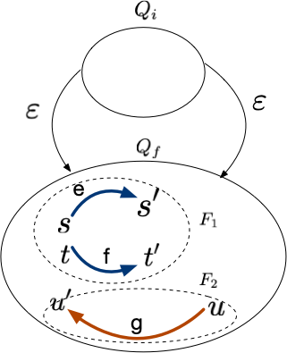
Figure 1: LDGBA with acceptance sets $F_{1},F_{2}$.

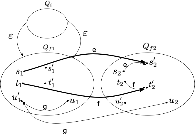
Figure 2: Equivalent LDBA with acceptance set $F^{\prime}$.

Occupancy Measures. Occupancy measures [26] allow formulating the problem of finding an optimal MDP policy as a linear program (LP) [26, 44].

Discounted-Reward MDP. For a discounted MDP $\mathcal{M}=(S,A,P,s_{0},\gamma,r)$, the occupancy measure $y^{\pi}:\mathbb{R}^{|S|\times|A|}\to\mathbb{R}_{\geq 0}$ of a stationary policy $\pi$ is defined as $y_{sa}^{\pi}=\sum_{t=0}^{\infty}\gamma^{t}P_{\pi}(S_{t}=s,A_{t}=a),$ where $P_{\pi}(S_{t}=s,A_{t}=a)$ denotes the probability of being in state $s$ and taking action $a$ at time $t$ under policy $\pi$. In words, $y_{sa}^{\pi}$ is the (discounted) expected number of visits to state-action pair $(s,a)$ under policy $\pi$. The following linear inequalities,

$$y_{sa}\geq 0\quad\forall s\in S\ \forall a\in A(s),$$ (1)

$$out(s)-in(s)=\mathds{1}_{s_{0}}(s)\quad\forall s\in S,$$

$$out(s)=\sum_{a\in A(s)}y_{sa}\quad\quad\forall s\in S,$$

$$in(s)=\gamma\sum_{j\in S,a\in A(j)}y_{ja}P(j,a,s)\quad\forall s\in S,$$

specify necessary and sufficient conditions for $y$ to be an occupancy measure for a discounted MDP $\mathcal{M}$ [26], where $out(s)$ and $in(s)$ denote the total outflow from, and inflow into, state $s$, respectively. The above inequalities can be interpreted as establishing the conservation of flow through each state. Moreover, the expected discounted reward under a stationary policy with occupancy measure $y$ can be expressed as $\sum_{s\in S}\sum_{a\in A(s)}r(s,a)y_{sa}$.

A corresponding stationary policy can be derived from an occupancy measure $y$ by setting $\pi(s,a)$ to be equal to $y_{sa}/\sum_{a\in A(s)}y_{sa}$ if $\sum_{a\in A(s)}y_{sa}>0$, or arbitrary otherwise. Therefore, inequalities (1) characterize the set of all stationary policies for $\mathcal{M}$.

Absorbing MDP. An occupancy measure can also be defined for an absorbing MDP $\mathcal{M}_{g}=(S,A,P,s_{0})$, that is, an MDP for which there exist a policy and a goal (absorbing) state $s_{g}\in S$ such that $s_{g}$ is reached almost surely. For an absorbing MDP $\mathcal{M}_{g}$ and policy $\pi$, an occupancy measure $x^{\pi}:\mathbb{R}^{(|S|-1)\times|A|}\to\mathbb{R}_{\geq 0}$ can be defined [26] as $x_{sa}^{\pi}=\sum_{t=0}^{\infty}P_{\pi}(S_{t}=s,A_{t}=a),\quad\forall s\in S\setminus\{s_{g}\}$, interpreted as the expected number of visits to the state-action pair $(s,a)$ under policy $\pi$ before reaching the goal state. The measure is finite, as the goal state $s_{g}$ is reached almost surely.

Similarly to the case of discounted MDPs, the following set of linear inequalities

$$x_{sa}\geq 0\quad\forall s\in S\setminus\{s_{g}\}\ \forall a\in A(s),$$

$$out(s)-in(s)=\mathds{1}_{s_{0}}(s)\quad\forall s\in S\setminus\{s_{g}\},$$

$$in(s_{g})=1,$$ (2)

$$out(s)=\sum_{a\in A(s)}x_{sa}\quad\quad\forall s\in S\setminus\{s_{g}\},$$

$$in(s)=\sum_{j\in S,a\in A(j)}x_{ja}P(j,a,s)\quad\forall s\in S,$$

specify necessary and sufficient conditions for $x$ to be an occupancy measure, where $out(s)$ and $in(s)$ are interpreted as in (1) and $in(s_{g})=1$ ensures the almost sure reachability of the goal state. It is also possible to derive a corresponding stationary policy from an occupancy measure as described above. Therefore, the linear inequalities (III) characterize the set of all stationary policies for $\mathcal{M}_{g}$ under which the goal state is reached almost surely.

IV Problem Formulation and Solution Strategy

We aim to synthesize a policy $\pi$ for an MDP $\mathcal{M}$ that is optimal with respect to an expected discounted reward under the constraint that an LTL formula $\varphi$ is satisfied with probability 1. We make the following assumption which can be easily verified by using standard techniques from probabilistic model checking [45].

Assumption 1.

For the given MDP $\mathcal{M}$ and LTL formula $\varphi$, there exists a policy such that the formula is satisfied with probability 1.

We now introduce the methodology used to solve the above objective as illustrated in Fig. 3. By representing the satisfaction of $\varphi$ with an LDBA $\mathcal{A}$ and leveraging a standard construction from LTL model checking of MDPs [27], we generate a product MDP $\mathcal{M}\times\mathcal{A}$ as the composition of $\mathcal{M}$ and $\mathcal{A}$, such that almost sure satisfaction of a Büchi acceptance condition on the product MDP, shown to be possible by Assumption 1, implies the almost sure satisfaction of $\varphi$ on the original MDP. As further discussed in Section IV-A, it is sufficient to consider the set of stationary deterministic policies $\Pi_{d}^{\times}$ of the product MDP to find a policy satisfying the Büchi acceptance condition almost surely. Let $\Pi_{d}$ be the projection of $\Pi_{d}^{\times}$ onto the policy space of the original MDP $\mathcal{M}$. Assumption 1 guarantees that a feasible policy exists in $\Pi_{d}$. We are then interested in the following problem:

$$\underset{\pi\in\Pi_{d}}{\text{ max }} {\mathcal{R}}_{\mathcal{M}}(\pi)$$ (3)

$$\mathrm{s.t.} Pr_{\pi}^{\mathcal{M}}(\varphi)=1.$$

By building on a result from Hahn et al. [18], we reduce the almost sure satisfaction of a Büchi acceptance condition on the product MDP to an almost sure reachability problem. We then introduce two occupancy measures to express both the reachability constraint and the discounted reward, and formulate a set of mixed integer linear constraints to guarantee that the occupancy measures are well defined and are both associated with the same deterministic policy. The solution of the resulting MILP provides the desired policy. In the following, we detail the above steps.

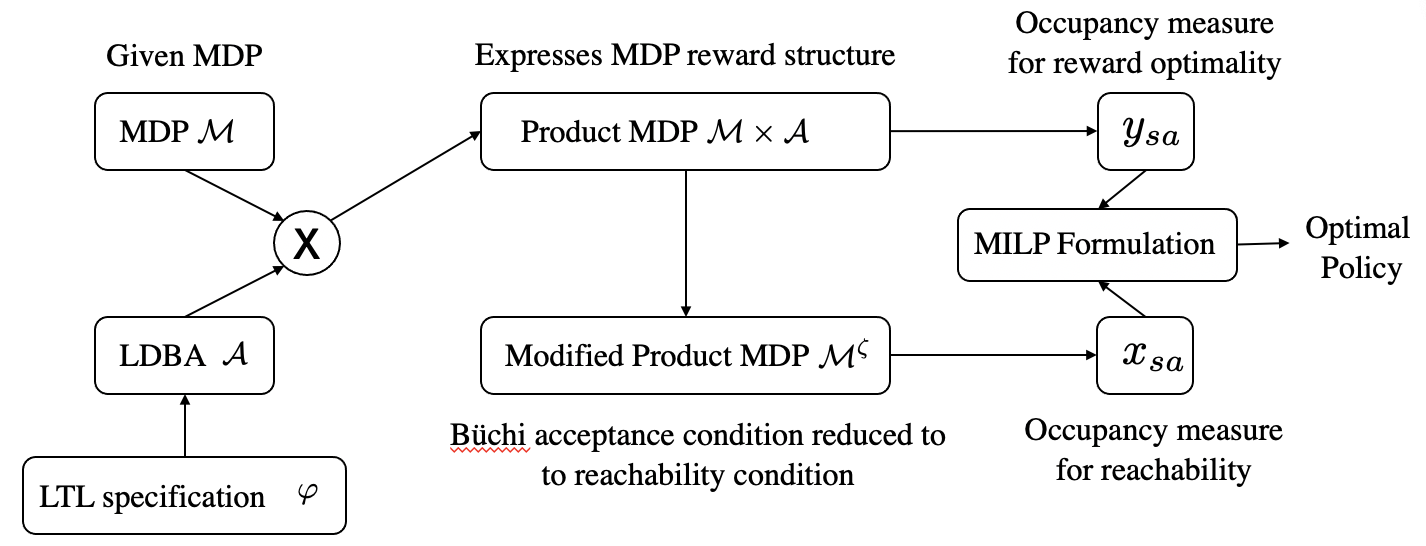
Figure 3: Flowchart describing the solution approach.

IV-A Construction of the Product MDP

Given an MDP $\mathcal{M}=(S,A,P,s_{0},\gamma,AP,L,r)$ and an LDBA $\mathcal{A}$ = $(Q,\Sigma,q_{0},\delta,F)$ capturing the LTL formula $\varphi$, where $Q=Q_{i}\cup Q_{f}$, we follow the construction in [27] to define a product MDP ($\mathcal{M}\times\mathcal{A}$) $\mathcal{M}^{\times}=(S^{\times},A^{\times},P^{\times},s_{0}^{\times},\gamma,r^{\times},F^{\times})$ which incorporates the transitions of $\mathcal{M}$ and $\mathcal{A}$, the reward function of $\mathcal{M}$ and the acceptance set of $\mathcal{A}$. The following running example illustrates the construction involved in our algorithm.

Example IV.1.

Consider the four state grid world MDP in Fig. 5. Each state associated with a location of the grid is labelled with the set of atomic propositions in $\{l_{0},l_{1},m\}$, that are true in it. The transition diagram of the MDP is shown in Fig. 5. The initial state is III. The actions $\mathsf{rest}$ (denoted by red transition arrows) and $\mathsf{go}$ (denoted by green transition arrows) are available in each state. Action $\mathsf{rest}$ does not change the state of the MDP. With action $\mathsf{go}$, the agent moves horizontally, in the same row, with probability $p$ or vertically, in the same column, with probability $1-p$.

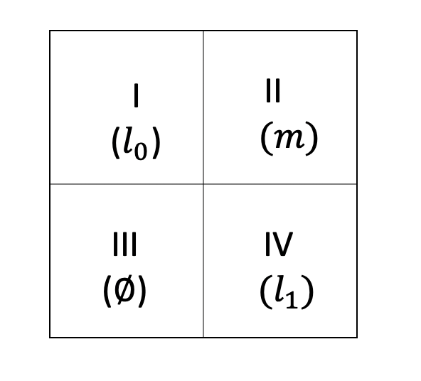
Figure 4: Grid world example.

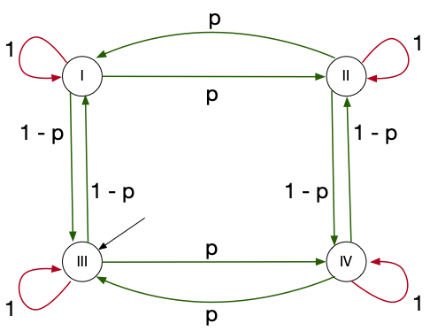
Figure 5: MDP transition diagram.

We wish to satisfy the LTL formula $\varphi:=(\textbf{FG}l_{0}\vee\textbf{FG}l_{1})\wedge\textbf{G}\neg m$, requiring to reach one of the safe cells (where $l_{0}$ or $l_{1}$ is true) and stay there forever, while avoiding the unsafe cell, where $m$ holds. An equivalent LDBA for this LTL formula is shown in Fig. 6. The transitions are labelled by propositional formulae which are equivalent to the Boolean assignments of the atomic propositions $\{l_{0},l_{1},m\}$ which satisfy the propositional formulae. The initial state is $0$ and the accepting transitions are marked in bold.

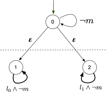
Figure 6: LDBA for $\varphi:=(\textbf{FG}l_{0}\vee\textbf{FG}l_{1})\wedge\textbf{G}\neg m$

The only non-deterministic transitions are the $\epsilon$ transitions from $Q_{i}=\{0\}$ to $Q_{f}=\{1,2\}$, where $Q_{i}\cap Q_{f}=\emptyset$ and $Q_{i}\cup Q_{f}=Q=\{0,1,2\}$. Further, $F\subseteq Q_{f}\times\Sigma\times Q_{f}$ holds, and there are no transitions from $Q_{f}$ to $Q_{i}$. As denoted by the dotted line, the states can be partitioned into $Q_{i}$ and $Q_{f}$.

In the product MDP $\mathcal{M}^{\times}$, $S^{\times}=S\times Q$ is the set of states, $A^{\times}=A\cup E$ is the action set, where $E=\{\epsilon_{q}|q\in Q_{f}\}$ is the set of actions which simulate $\epsilon$-transitions to states in $Q_{f}$, and $s_{0}^{\times}=(s_{0},q_{0})$ is the initial state. We then define the transition function $P^{\times}((s,q),a,(s^{\prime},q^{\prime}))$ as follows

$$\begin{cases}P(s,a,s^{\prime}),&\mbox{if }q^{\prime}=\delta(q,L(s))\text{ and }a\not\in E,\\ 1,&\mbox{if }s=s^{\prime},\quad a=\epsilon_{q^{\prime}},\quad q^{\prime}\in\delta(q,\epsilon),\\ 0,&\text{otherwise.}\end{cases}$$ (4)

and the reward function as

$$r^{\times}((s,q),a) =\begin{cases}r(s,a),&\mbox{if }a\not\in E,q\in Q_{i},\\ r(s,a)/\gamma,&\mbox{if }a\not\in E,q\in Q_{f},\\ 0,&\text{otherwise.}\end{cases}$$ (5)

Finally, the set of accepting transition of $\mathcal{M}^{\times}$ includes the non-zero probability transitions of $\mathcal{M}^{\times}$ capturing the accepting transitions of $\mathcal{A}$, i.e., $F^{\times}=\{((s_{i},q_{i}),a,(s_{j},q_{j}))|(q_{i},L(s_{i}),q_{j})\in F,P(s_{i},a,s_{j})>0\}$.

Example IV.2.

Fig. 7 shows the product MDP $\mathcal{M}^{\times}$ between $\mathcal{M}$ and $\mathcal{A}$ in Example IV.1.

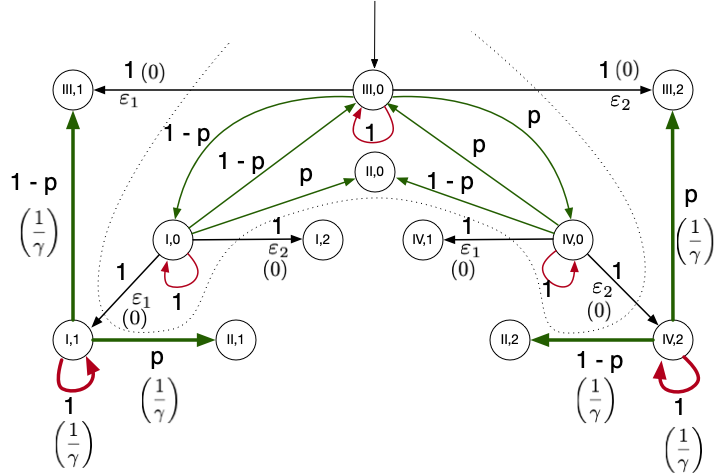
Figure 7: Product MDP $\mathcal{M}^{\times}$.

The $\mathsf{rest}$, $\mathsf{go}$, and $\epsilon$ actions are denoted by red, green, and black arrows, respectively. The accepting transitions $F^{\times}$ are in bold. The rewards associated with the discounted reward objective are obtained as follows. Epsilon actions $\epsilon_{1}$ and $\epsilon_{2}$ are associated with $0$ reward (in brackets). The rewards associated with transitions from states $(s,q)$, $q\in Q_{f}$, are multiplied by $\frac{1}{\gamma}$ to compensate for the artificial increase in time step and additional discounting due to the $\epsilon$-transition, as further detailed below. We observe that, differently from previous work [18, 19, 20], the expected discounted reward in our setting is associated with a user-defined objective function and is unrelated to the LTL reachability objective.

A run $\xi^{\times}$ of $\mathcal{M}^{\times}$ is said to satisfy the Büchi acceptance condition $\varphi_{F^{\times}}$ if $\inf(\xi^{\times})\cap F^{\times}\neq\emptyset$, i.e., there exists a transition belonging to $F^{\times}$ that occurs infinitely often in $\xi^{\times}$. The probability that a run of $\mathcal{M}^{\times}$ starting from the initial state $s_{0}^{\times}$ under policy $\pi^{\times}$ satisfies the Büchi acceptance condition $\varphi_{F^{\times}}$ is denoted by $Pr_{\pi^{\times}}^{\mathcal{M}^{\times}}(\varphi_{F^{\times}})$.

The transition function in (4) represents the effect of $\epsilon$-transitions in $\mathcal{A}$, which are the only non-deterministic transitions, in terms of actions $\epsilon_{q^{{}^{\prime}}}$ that cause the current state $(s,q)$ to transition to a state $(s^{\prime},q^{\prime})$, where $q^{\prime}$ is the destination of the corresponding $\epsilon$-transition in $\mathcal{A}$, while $s^{\prime}=s$, meaning that no change in the corresponding state of $\mathcal{M}$ takes place. Only when an action $a\not\in E$ is taken, the corresponding state $s$ of $\mathcal{M}$ is updated based on the transition probability $P(s,a,s^{\prime})$, while $q$ is updated as determined by the corresponding transition function $\delta$ of $\mathcal{A}$ and the label $L(s)$ associated with $s$.

We observe that a run $\xi^{\times}$ of $\mathcal{M}^{\times}$ can contain at most one $\epsilon$-transition, corresponding to a jump from $Q_{i}$ to $Q_{f}$ in $\mathcal{A}$. A run $(s_{0},q_{0})a_{0}(s_{1},q_{1})a_{1}\ldots(s_{l},q_{l})\epsilon_{q_{l+1}}(s_{l+1},q_{l+1})a_{l+1}\ldots$, with $s_{l+1}=s_{l}$, corresponds to the run $s_{0},a_{0},s_{1},a_{1},\ldots,s_{l-1},a_{l-1},s_{l},a_{l+1},s_{l+2},a_{l+2},\ldots$ of $\mathcal{M}$, where we observe that an $\epsilon$-action in $\mathcal{M}^{\times}$ does not reflect into a change of state for $\mathcal{M}$. The additional division by $\gamma$ introduced in (5) compensates for the discounting caused by the $\epsilon$-transition in $\mathcal{M}^{\times}$ and the resulting additional time-step, as stated by the lemma below.

Lemma 1.

Given an MDP $\mathcal{M}=(S,A,P,s_{0},\gamma,AP,L,r)$, an LTL formula $\varphi$, and an LDBA $\mathcal{A}=(Q,\Sigma,q_{0},\delta,F)$ equivalent to $\varphi$, let $\mathcal{M}^{\times}=\mathcal{M}\times\mathcal{A}$. The total discounted reward of a run $\xi^{\times}$ of $\mathcal{M}^{\times}$ is equal to the total discounted reward of $\xi$, obtained by projecting $\xi^{\times}$ to the state and action spaces of $\mathcal{M}$.

Proof.

We consider two cases, based on whether $\xi^{\times}$ contains an $\epsilon$-transition or not. Let us first assume that $\xi^{\times}$ does not contain $\epsilon$-transitions. Then, by (5) and the fact that $q_{n}\in Q_{i}$ for all $n\geq 0$, we obtain

$$\sum_{n=0}^{\infty}{\gamma}^{n}r^{\times}((s_{n},q_{n}),a_{n})=\sum_{n=0}^{\infty}{\gamma}^{n}r(s_{n},a_{n}).$$

This implies that $G_{\mathcal{M}^{\times}}(\xi^{\times})=G_{\mathcal{M}}(\xi)$, i.e., the total discounted reward of $\xi^{\times}$ is equal to that of its projection $\xi^{\times}$ to the state and action spaces of $\mathcal{M}$.

Assume now that $\xi^{\times}$ contains an $\epsilon$-transition, that is, given $\xi^{\times}=(s_{0},q_{0})a_{0}\ldots(s_{l},q_{l})a_{l}(s_{l+1},q_{l+1})\ldots$, we have $a_{l}=\epsilon_{q_{l+1}}$ and $s_{l+1}=s_{l}$. Then, by (5), we obtain

$$\sum_{n=0}^{\infty}{\gamma}^{n}r^{\times}((s_{n},q_{n}),a_{n})=\sum_{n=0}^{l-1}{\gamma}^{n}r^{\times}((s_{n},q_{n}),a_{n}))+$$

$$\qquad+{\gamma}^{l}r^{\times}((s_{l},q_{l}),\epsilon_{q_{l+1}})+\sum_{n=l+1}^{\infty}{\gamma}^{n}r^{\times}((s_{n},q_{n}),a_{n}),$$

where $q_{n}\in Q_{i}$ for $n\leq l$ and $q_{n}\in Q_{f}$ for $n>l$. Further, by observing that $s_{l+1}=s_{l}$, and $r^{\times}((s_{l},q_{l}),\epsilon_{q_{l+1}})=0$, we obtain

$$\sum_{n=0}^{\infty}{\gamma}^{n}r^{\times}((s_{n},q_{n}),a_{n})=\sum_{n=0}^{l-1}{\gamma}^{n}r(s_{n},a_{n})+$$

$$(1/\gamma)(\sum_{n=l+1}^{\infty}{\gamma}^{n}r(s_{n},a_{n}))$$

which is the total discounted reward associated with the run $\xi:(s_{0},a_{0},\ldots,s_{l-1},a_{l-1},s_{l},a_{l+1},s_{l+2},a_{l+2},\ldots)$. Again, we conclude $G_{\mathcal{M}^{\times}}(\xi^{\times})=G_{\mathcal{M}}(\xi)$, which is what we wanted to prove. ∎∎

By Theorem $3$ in [27], it is sufficient to focus on stationary policies of $\mathcal{M}^{\times}$ to maximize the probability of satisfaction of the LTL formula $\varphi$. We restate this result in Lemma 2 below.

Lemma 2.

For $\mathcal{M}$ and $\mathcal{M}^{\times}$ as defined in Lemma 1, any stationary policy $\pi^{\times}_{*}$ of $\mathcal{M}^{\times}$ which maximizes the probability of satisfying the Büchi acceptance condition $Pr_{\pi^{\times}}^{\mathcal{M}^{\times}}(\varphi_{F^{\times}})$ in $\mathcal{M}^{\times}$ induces a finite memory policy $\pi_{*}$ on $\mathcal{M}$ such that $\pi_{*}$ maximizes the probability of LTL satisfaction $Pr_{\pi}^{\mathcal{M}}(\varphi)$ and $Pr_{\pi^{\times}_{*}}^{\mathcal{M}^{\times}}(\varphi_{F^{\times}})=Pr_{\pi_{*}}^{\mathcal{M}}(\varphi)$ holds.

A stationary policy $\pi^{\times}$ for $\mathcal{M}^{\times}$ can be mapped to $\pi$ for $\mathcal{M}$ as follows. $\mathcal{M}$ and $\mathcal{A}$ start from states $s_{0}$ and $q_{0}$, respectively. Whenever $\mathcal{M}$ transitions from $s$ to $s^{\prime}$ on action $a\in A(s)$, $\mathcal{A}$ updates its state to $\delta(q,L(s))$. For states $s$ of $\mathcal{M}$ and $q$ of $\mathcal{A}$, action $a\in A^{\times}$ is selected with probability $\pi^{\times}((s,q),a)$. If the selected action is an $\epsilon$-action $\epsilon_{q^{\prime}}$, then the state of $\mathcal{A}$ is updated to $q^{\prime}$ while $\mathcal{M}$ keeps the same state and selects the next action $a\in A$ with probability $\pi^{\times}((s,q^{\prime}),a)$. Else, both $\mathcal{M}$ and $\mathcal{A}$ progress based on their transition function. Therefore, $\pi$ prescribes an action given the current state of $\mathcal{M}$ and $\mathcal{A}$ based on $\pi^{\times}$.

By Lemma 2 and Assumption 1, there exist stationary policies for $\mathcal{M}^{\times}$ such that $Pr_{\pi^{\times}}^{\mathcal{M}^{\times}}(\varphi_{F^{\times}})=Pr_{\pi}^{\mathcal{M}}(\varphi)=1$. Moreover, in Section IV-B, $Pr_{\pi^{\times}}^{\mathcal{M}^{\times}}(\varphi_{F^{\times}})=1$ is shown to be equivalent to an almost sure reachability, for which optimal deterministic stationary policies are guaranteed to exist [3]. We can then look for a deterministic stationary policy $\pi^{\times}$ such that $Pr_{\pi^{\times}}^{\mathcal{M}^{\times}}(\varphi_{F^{\times}})=1$ and ${\mathcal{R}}_{\mathcal{M}^{\times}}(\pi^{\times})$ is maximized. Finally, by Lemma 1 and the construction of the product MDP, we have that ${\mathcal{R}}_{\mathcal{M}}(\pi)={\mathcal{R}}_{\mathcal{M}^{\times}}(\pi^{\times})$ holds, and Problem (3) reduces to the following problem:

$$\underset{\pi^{\times}\in\Pi_{d}^{\times}}{\text{ max }} {\mathcal{R}}_{\mathcal{M}^{\times}}(\pi^{\times})$$ (6)

$$\mathrm{s.t.} Pr_{\pi^{\times}}^{\mathcal{M}^{\times}}(\varphi_{F^{\times}})=1.$$

IV-B Reachability Reduction of Büchi Acceptance

Recent work [18] has shown that a modified product MDP $\mathcal{M}^{\zeta}$ can be generated from $\mathcal{M}^{\times}$ such that almost sure satisfaction of the Büchi acceptance condition is equivalent to almost sure reachability of a new absorbing state in $\mathcal{M}^{\zeta}$.

The modified product MDP $\mathcal{M}^{\zeta}$ is defined as $(S^{\zeta},A^{\zeta},P^{\zeta},s_{0}^{\zeta})$, where $S^{\zeta}=S^{\times}\cup\{g\}$, $A^{\zeta}=A^{\times}$ and $s_{0}^{\zeta}=s_{0}^{\times}$. $\mathcal{M}^{\zeta}$ is constructed from $\mathcal{M}^{\times}$ by adding a new absorbing state $g$ to $S^{\times}$. Given $\zeta\in(0,1)$, $P^{\zeta}$ is obtained from $P^{\times}$ as follows. For each accepting transition $((s_{i},q_{i}),a,(s_{j},q_{j}))\in F^{\times}$, $g$ becomes the destination of the transition with probability $1-\zeta$, while the probabilities of reaching all the other possible destinations on taking action $a$ in $(s_{i},q_{i})$ are multiplied by $\zeta$.

Example IV.3.

Fig.8 shows the MDP $\mathcal{M}^{\zeta}$ obtained by modifying the product MDP $\mathcal{M}^{\times}$ in Fig. 7 to add a new absorbing state $g$ and modified accepting transitions as described above. The new transitions in $\mathcal{M}^{\zeta}$ are marked by dot-dash lines. $\mathcal{M}^{\zeta}$ does not have an associated reward function and is only used to express the almost satisfaction of the given LTL formula. On the other hand, $\mathcal{M}^{\times}$ in Fig. 7 is used to express the discounted-reward objective.

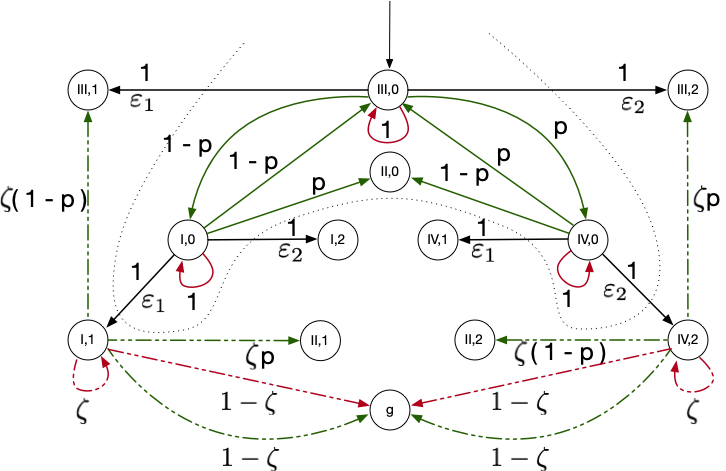
Figure 8: Modified product MDP $\mathcal{M}^{\zeta}$.

We observe that $\mathcal{M}^{\zeta}$ and $\mathcal{M}^{\times}$ have a common set of states $S^{\times}$ except for the absorbing state $g$ in $S^{\zeta}$. Therefore, a single stationary policy can be defined for both $\mathcal{M}^{\zeta}$ and $\mathcal{M}^{\times}$ over $S^{\times}$. Let $\rho_{\pi^{\times}}^{\zeta}(t)$ denote the probability of reaching $g$ in $\mathcal{M}^{\zeta}$ by following policy $\pi^{\times}$. The following lemmas relate the probability of reaching $g$ in $\mathcal{M}^{\zeta}$ with the probability of satisfying the LTL formula $\varphi$, i.e., of satisfying the associated Büchi acceptance condition in $\mathcal{M}^{\times}$. Lemma 3 below follows from Lemma 1 [18].

Lemma 3.

For $\mathcal{M}$ and $\mathcal{M}^{\times}$ as defined in Lemma 1, let $\mathcal{M}^{\zeta}=(S^{\zeta},A^{\zeta},P^{\zeta},s_{0}^{\zeta})$ be the modified absorbing product MDP. For $\zeta\in(0,1)$ and a stationary policy $\pi^{\times}$ in $\mathcal{M}^{\zeta}$, we obtain $\rho_{\pi^{\times}}^{\zeta}(t)\geq Pr_{\pi^{\times}}^{\mathcal{M}^{\times}}(\varphi_{F^{\times}})$. Moreover, $\rho_{\pi^{\times}}^{\zeta}(t)=1$ implies $Pr_{\pi^{\times}}^{\mathcal{M}^{\times}}(\varphi_{F^{\times}})=1$.

In the case of almost sure satisfaction, Lemma 3 reduces to the following result:

Lemma 4.

For $\mathcal{M}$ and $\mathcal{M}^{\times}$ as defined in Lemma 1, let $\mathcal{M}^{\zeta}=(S^{\zeta},A^{\zeta},P^{\zeta},s_{0}^{\zeta})$ be the modified absorbing product MDP. For $\zeta\in(0,1)$ and a stationary policy $\pi^{\times}$ in $\mathcal{M}^{\zeta}$, $\rho_{\pi^{\times}}^{\zeta}(t)=1$ if and only if $Pr_{\pi^{\times}}^{\mathcal{M}^{\times}}(\varphi_{F^{\times}})=1$.

Proof.

If $\pi^{\times}$ is such that $\rho_{\pi^{\times}}^{\zeta}(t)=1$, then $Pr_{\pi^{\times}}^{\mathcal{M}^{\times}}(\varphi_{F^{\times}})=1$ by Lemma 3. Also, it is obvious from Lemma 3 that $Pr_{\pi^{\times}}^{\mathcal{M}^{\times}}(\varphi_{F^{\times}})=1$ implies $\rho_{\pi^{\times}}^{\zeta}(t)=1$. ∎∎

We conclude that the set of stationary deterministic policies of $\mathcal{M}^{\times}$ which satisfy the Büchi acceptance condition almost surely is equal to the set of stationary deterministic policies of $\mathcal{M}^{\zeta}$ for which the absorbing state $g$ is reached almost surely.

IV-C Occupancy Measures

From Lemmas 2 and 4, almost sure satisfaction of an LTL constraint on $\mathcal{M}$ can be expressed as an almost sure reachability constraint on $\mathcal{M}^{\zeta}$. However, this reachability constraint can also be expressed in terms of the occupancy measure $x_{sa}$ defined on the absorbing MDP $\mathcal{M}^{\zeta}$ as discussed Section III:

$$x_{sa}\geq 0\quad\forall s\in S^{\times}\ \forall a\in A^{\times}(s),$$ (7)

$$out^{x}(s)-in^{x}(s)=\mathds{1}_{s_{0}^{\times}}(s)\quad\forall s\in S^{\times},$$

$$in^{x}(g)=1\quad\quad\quad g\in S^{\zeta},$$

$$out^{x}(s)=\sum_{a\in A^{\times}(s)}x_{sa}\quad\quad\forall s\in S^{\times},$$

$$in^{x}(s)=\sum_{j\in S^{\times},a\in A^{\times}(j)}x_{ja}P^{\zeta}(j,a,s)\quad\forall s\in S^{\zeta}.$$

Similarly, the discounted reward optimization problem on $\mathcal{M}^{\times}$ can be expressed in terms of an occupancy measure $y_{sa}$ $\mathcal{M}^{\times}$ as follows:

$$y_{sa}\geq 0\quad\forall s\in S^{\times}\ \forall a\in A^{\times}(s),$$ (8)

$$out^{y}(s)-in^{y}(s)=\mathds{1}_{s_{0}^{\times}}(s)\quad\forall s\in S^{\times},$$

$$out^{y}(s)=\sum_{a\in A^{\times}(s)}y_{sa},\quad\quad\forall s\in S^{\times},$$

$$in^{y}(s)=\gamma\sum_{j\in S^{\times},a\in A^{\times}(j)}y_{ja}P^{\times}(j,a,s)\quad\forall s\in S^{\times}.$$

while the expected discounted reward under policy $\pi^{\times}$ with occupancy measure $y_{sa}$ is ${\mathcal{R}}_{\mathcal{M}^{\times}}({\pi}^{\times})=\sum_{s\in S^{\times},a\in A^{\times}(s)}r^{\times}(s,a)y_{sa}.$

Finally, we need to ensure that both occupancy measures originate from the same underlying policy $\pi^{\times}$, which maximizes the reward and satisfies the LTL specification. We then require that ${x_{sa}}/{\sum_{a^{{}^{\prime}}\in A^{\times}(s)}x_{sa^{{}^{\prime}}}}={y_{sa}}/{\sum_{a^{{}^{\prime}}\in A^{\times}(s)}y_{sa^{{}^{\prime}}}},$ for all $a\in A^{\times}(s)$ and $s\in S^{\times}$. We achieve this equality by introducing a set of binary variables and constraints to restrict the search to the space of deterministic policies as detailed in the next section.

IV-D Mixed Integer Linear Program Formulation

For all the states shared by $\mathcal{M}^{\times}$ and $\mathcal{M}^{\zeta}$ and the associated actions, i.e., for all $s\in S^{\times}$ and $a\in A^{\times}(s)$, we introduce binary variables $\Delta_{sa}\in\{0,1\}$ that evaluate to $1$ if and only if action $a$ is selected in visited state $s$. By using these binary variables, we can require that a policy is deterministic via the following constraint:

$$\sum_{a}\Delta_{sa}\leq 1\quad\forall s\in S^{\times},$$ (9)

meaning that at most one action $a$ can be selected in state $s$. We can then require the equivalence between the occupancy measures defined in Section IV-C using the following logical constraints:

$$(\Delta_{sa}=0)\to(x_{sa}=0)\quad\forall s\in S^{\times},\ \forall a\in A^{\times},$$ (10a)

$$(\Delta_{sa}=0)\to(y_{sa}=0)\quad\forall s\in S^{\times},\ \forall a\in A^{\times},$$ (10b)

where $\to$ denotes the logical implication. These constraints can be converted into mixed integer linear constraints using standard techniques [46]. A similar idea was previously used to generate deterministic policies for constrained MDPs [47].

The policies generated by the occupancy measures are deterministic under constraints (9)-(10) as stated by the following lemmas.

Lemma 5.

Given a discounted MDP $\mathcal{M}^{\times}$, a stationary policy $\pi^{\times}$, the associated occupancy measure $y_{sa}$, binary variables $\Delta_{sa}$, $\forall s\in S^{\times},\ \forall a\in A^{\times}$, if $y$ and $\Delta$ satisfy equations (9)-(10), then for all states $s\in S^{\times}$ visited with non-zero probability, policy $\pi^{\times}$ is deterministic and, further, $y_{sa}>0$ if and only if $\Delta_{sa}=1$.

Proof.

Consider a state $s^{*}\in S^{\times}$ which is visited with non-zero probability under policy $\pi^{\times}$. We obtain the following chain of implications:

$$\sum_{a\in A^{\times}(s^{*})}y_{s^{*}a}>0\implies\exists a^{*}\in A^{\times}(s^{*})\ \text{s.t.}\ y_{s^{*}a^{*}}>0$$

$$\implies\Delta_{s^{*}a^{*}}=1\text{ by \eqref{gyzero}}$$

$$\implies\Delta_{s^{*}a}=0\quad\forall a\neq a^{*}\text{ by \eqref{deter}}$$

$$\implies y_{s^{*}a}=0\quad\forall a\neq a^{*}\text{ by \eqref{gyzero}}$$

$$\implies\pi^{\times}(s^{*},a^{*})=1\quad\text{and}\quad\pi^{\times}(s^{*},a)=0\quad\forall a\neq a^{*}$$

$$\implies\pi^{\times}\text{ is deterministic.}$$

Therefore, if $s$ is visited with non-zero probability, $y_{sa}>0$ if and only if $\Delta_{sa}=1$. ∎∎

Similarly, the following lemma can be stated for the absorbing MDP $\mathcal{M}^{\zeta}$.

Lemma 6.

Given an absorbing MDP $\mathcal{M}^{\zeta}$, a stationary policy $\pi^{\times}$, the associated occupancy measure $x_{sa}$, binary variables $\Delta_{sa}$, $\forall s\in S^{\times},\ \forall a\in A^{\times}$, if $x$ and $\Delta$ satisfy equations (9)-(10), then for all states $s\in S^{\zeta}\setminus\{g\}$ visited with non-zero probability, policy $\pi^{\times}$ is deterministic and, further, $x_{sa}>0$ if and only if $\Delta_{sa}=1$.

The following lemma shows that under constraints (9)-(10), the set of reachable states in $S^{\times}$ under policies given by $x$ and $y$ are the same and have the same deterministic action choices on those states.

Lemma 7.

Given an MDP $\mathcal{M}^{\times}$, a stationary policy $\pi^{y}$, the associated occupancy measure $y_{sa}$, the absorbing MDP $\mathcal{M}^{\zeta}$ generated from $\mathcal{M}^{\times}$, a stationary policy $\pi^{x}$, the associated occupancy measure $x_{sa}$, binary variables $\Delta_{sa}$, $\forall s\in S^{\times},\ \forall a\in A^{\times}$, if $x,y$ and $\Delta$ satisfy equations (9)-(10), then the set of reachable states in $S^{\times}$ under $\pi_{x}$ and $\pi_{y}$ and the deterministic action choices on those states are the same.

Proof.

$\mathcal{M}^{\times}$ and $\mathcal{M}^{\zeta}$ have the same initial state $(s_{0},q_{0})$, which is clearly visited for both the MDPs. Therefore, from the proof of Lemma 5, $\exists a^{*}\text{ such that }\Delta_{(s_{0},q_{0}),a^{*}}=1$ and $\Delta_{(s_{0},q_{0}),a}=0\ \forall a\neq a^{*}$. From Lemma 5 and Lemma 6, we also have $x_{(s_{0},q_{0}),a^{*}}>0,y_{(s_{0},q_{0}),a^{*}}>0$ as well as $x_{(s_{0},q_{0}),a}=0,y_{(s_{0},q_{0}),a}=0,\forall a\neq a^{*}$. Therefore, both the occupancy measures provide the same action $a^{*}$ in the initial state.

The set of states reachable in $S^{\times}$ after one step, that is, after selecting $a^{*}$ in the initial state, is the same for both $\mathcal{M}^{\times}$ and $\mathcal{M}^{\zeta}$ by the construction of the transition probabilities $P^{\zeta}$ from $P^{\times}$. In fact, the transition probabilities between states of $S^{\times}$ are scaled by non-zero constants, which does not change their reachability. Similarly to the argument above, both occupancy measures propose the same actions in all the states reachable in $S^{\times}$ after one step. We can then proceed by induction to conclude that the set of reachable states in $S^{\times}$ for $\mathcal{M}^{\times}$ and $\mathcal{M}^{\zeta}$ are the same for $n$ steps, $n\geq 0$, and both the occupancy measures determine the same actions in all the reachable states in $S^{\times}$. ∎∎

By putting together constraints (7)-(10) in terms of the binary variables, occupancy measures, and the expected discounted reward objective, we obtain the following MILP problem whose solution provides the desired policy:

$$\underset{x,y,\Delta\in\{0,1\}}{\text{ max }}\quad\sum_{s\in S^{\times},a\in A^{\times}(s)}r^{\times}(s,a)y_{sa},$$ (11)

$$\mathrm{s.t.}\quad x_{sa}\geq 0,\quad y_{sa}\geq 0\quad\forall s\in S^{\times}\ \forall a\in A^{\times}(s),$$

$$out^{y}(s)-in^{y}(s)=\mathds{1}_{s_{0}^{\times}}(s)\quad\forall s\in S^{\times},$$

$$out^{x}(s)-in^{x}(s)=\mathds{1}_{s_{0}^{\times}}(s)\quad\forall s\in S^{\times},$$

$$in^{x}(g)=1\quad\quad\quad g\in S^{\zeta},$$

$$\sum_{a\in A^{\times}(s)}\Delta_{sa}\leq 1\quad\forall s\in S^{\times},$$

$$(\Delta_{sa}=0)\to(x_{sa}=0)\quad\forall s\in S^{\times}\ \forall a\in A^{\times}(s),$$

$$(\Delta_{sa}=0)\to(y_{sa}=0)\quad\forall s\in S^{\times}\ \forall a\in A^{\times}(s),$$

$$out^{y}(s)=\sum_{a\in A^{\times}(s)}y_{sa},\quad\quad\forall s\in S^{\times},$$

$$in^{y}(s)=\gamma\sum_{j\in S^{\times},a\in A^{\times}(j)}y_{ja}P^{\times}(j,a,s)\quad\forall s\in S^{\times},$$

$$out^{x}(s)=\sum_{a\in A^{\times}(s)}x_{sa}\quad\quad\forall s\in S^{\times},$$

$$in^{x}(s)=\sum_{j\in S^{\times},a\in A^{\times}(j)}x_{ja}P^{\zeta}(j,a,s)\quad\forall s\in S^{\zeta}.$$

The main result of this section can then be summarized by the following theorem.

Theorem 1.

Under Assumption 1, Problem (11) is feasible and provides an optimal deterministic policy for the formulated Problem (6). Specifically, if $\Delta_{sa}=1$, then the optimal deterministic policy requires to select action $a$ on visiting state $s$.

Problem (11) is feasible since a deterministic policy which reaches the absorbing state $g$ with probability 1 exists due to Assumption 1 and Lemmas 2 and 4. This deterministic policy on $\mathcal{M}^{\times}$ translates into a a finite-memory policy on $\mathcal{M}$ as discussed in Section IV-A.

IV-E Incorporating Additional Expected Discounted-Reward Constraints

In certain applications, it may be necessary to express additional constraints that can be captured in terms of lower bounds to expected total discounted returns $d_{i}$, $i=1,\ldots,n$, with respect to reward functions $r_{i}$ and discount factors $\gamma_{i}$ which are different from the primary function $r$ and discount factor $\gamma$, respectively. These constraints of the form

$${\mathbb{E}}_{\pi}\left[\sum_{t=0}^{\infty}{\gamma_{i}}^{t}r_{i}(s_{t},a_{t})\right]>d_{i},\quad i=1,\ldots,n$$

can be seamlessly incorporated within our formulation, by defining additional occupancy measures $y^{i}$, associated with $r_{i},\gamma_{i}$, $i=1,\ldots,n$, as

$$\sum_{s\in S^{\times},a\in A^{\times}(s)}r^{\times}(s,a)y^{i}_{sa}>d_{i}\quad i=1\ldots n$$

along with the necessary and sufficient conditions for $y^{i}$ to be an occupancy measure as in (8). Finally, we ensure that the occupancy measures originate from the same underlying policy by the following additional constraints, similar to the ones in Section IV-D:

$$(\Delta_{sa}=0)\to(y^{i}_{sa}=0)\quad\forall s\in S^{\times}\ \forall a\in A^{\times}(s).$$

V Experimental Results

We implemented the MILP-based framework in Python, using Rabinizer 4 [43] to generate an equivalent LDBA from an LTL formula and Gurobi for solving the MILPs. We evaluate the framework on two case studies involving motion planning of a mobile robot. The experiments are run on a $1.4$-GHz Core i5 processor with $16$-GB memory.

V-A Safe Motion Planning

We first consider a simple grid-world MDP that extends the MDP in Example IV.1, as shown in Fig. 9. Starting from initial state $0$, the robot tries to reach and remain in one of the safe cells (labeled with $l_{0}$ and $l_{1}$) while avoiding the unsafe cells (labeled with $m$). This task is formally specified by the LTL formula

$$(\textbf{F}\textbf{G}l_{0}\vee\textbf{FG}l_{1})\wedge\textbf{G}\neg m.$$

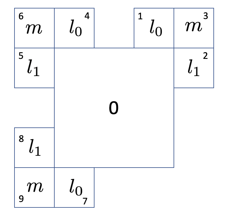
Figure 9: A grid-world MDP case study.

The action $\mathsf{rest}$ which does not change the MDP state is available to the robot in every location. Further, in the initial state $0$, the robot has three more actions available, namely, $\mathsf{ur}$ (upper right), $\mathsf{ul}$ (upper left), and $\mathsf{ll}$ (lower left) such that for $p>0$,

$$P(0,\mathsf{ur},1)=p, P(0,\mathsf{ur},2)=1-p,$$

$$P(0,\mathsf{ul},4)=p, P(0,\mathsf{ul},5)=1-p,$$

$$P(0,\mathsf{ll},7)=p, P(0,\mathsf{ll},9)=1-p$$

In the rest of the cells, the robot can also take action $\mathsf{move}$, by which the robot moves to the vertically adjoining cell with probability $p$ and to the horizontally adjoining cell with probability $1-p$.

Clearly, the deterministic policies which satisfy the LTL formula are of the following form: take an action $a\in\{\mathsf{ur},\mathsf{ul},\mathsf{ll}\}$ when in state $0$, and action $\mathsf{rest}$ in the other visited states. A reward function $r(s,a)$ gives rise to the expected discounted reward creating an ordering between the above described policies.

The LDBA generated from the LTL formula and the product MDP included 3 states and 30 states, respectively. The resulting MILP, including $173$ continuous and $86$ binary variables required less than $100$-ms runtime for various values of the parameter $p$, discount factor $\gamma$, and reward function $r(s,a)$. For all choices of the parameters, the generated MILP gives a policy of the form described above, which chooses to move to the quadrant offering maximum discounted reward.

V-B Nursery Scenario

In this grid-world example, the robot can take actions in the set $\{\mathsf{up,down,left,right}\}$ at each cell of a grid, as shown in Fig. 11 and Fig. 11. On taking each action, the robot moves in the intended direction with probability $0.8$ and sideways with total probability $0.2$, equally divided between the two directions (i.e., a probability of $0.1$ is allocated for moving in each side direction). If the robot is unable to move in a direction due to the presence of a wall, it remains in the same cell.

An adult, a baby, a charger, and a danger zone are present in four distinct cells of the grid, whose locations are indicated by the truth values of the atomic propositions $a$, $b$, $c$, and $d$, respectively, associated with each cell of the grid. For example, atomic proposition $a$ is true in cell $(x,y)$ if and only the adult is in cell $(x,y)$.

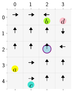
Figure 10: Nursery with equal
rewards for all actions (A).

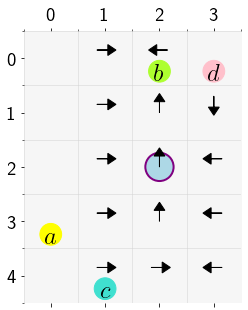
Figure 11: Nursery with lower
reward for action $\mathsf{up}$ (B).

The robot is initially at the charger. Its objective is to check on the baby repeatedly and get back to the charger after doing so, while always avoiding the danger zone. Due to the dynamics of the robot, in some cases, after checking on the baby, the robot remains in the same cell for more than one time step (represented by $b\wedge\textbf{X}b$ in LTL). This behavior disturbs the baby and requires the robot to notify (visit) the adult. This objective can be formally expressed in LTL as follows:

$$\varphi:=\textbf{G}[\underbrace{\neg d}_{\text{($i$)}}\wedge\underbrace{(c\to(\neg a\textbf{U}b))}_{\text{($ii$)}}\wedge\underbrace{(a\to\textbf{X}(\neg a\textbf{U}b))}_{\text{($iii$)}}\wedge$$ (12)

$$\underbrace{((\neg b\wedge\textbf{X}b\wedge\neg\textbf{X}\textbf{X}b)\to(\neg a\textbf{U}c))}_{\text{($iv$)}}\wedge\underbrace{((b\wedge\textbf{X}b)\to\textbf{F}a)}_{\text{($v$)}}\wedge$$

$$\underbrace{((b\wedge\neg\textbf{X}b)\to\textbf{X}(\neg b\textbf{U}(a\vee c)))}_{\text{($vi$)}}]$$

Sub-formulae $(i)$-$(vi)$ capture the following specifications which must always be true: $(i)$ avoid the region which is a danger zone; $(ii)$ if charged, visit the baby and do not visit the adult until then; $(iii)$ if the adult has been notified, visit the baby and do not visit the adult again until then; $(iv)$ if the baby has been checked on and left undisturbed, get charged and do not notify the adult until then; $(v)$ if the baby has been disturbed, eventually notify the adult; and $(vi)$ on leaving the baby, either notify the adult or charge and do not visit the baby again until then.

Optimal policies were synthesized by solving Problem (11) and simulated for a grid of size $5\times 4$ and discount factor $0.9$ in two scenarios marked with A and B, respectively. In both scenarios, in the location of the baby, all actions were assigned a reward of $10$. In scenario A, all actions are allocated the same reward of $2$ in the rest of the cells. In scenario B, all actions are allocated the same reward ($2$) except for action $\mathsf{up}$ which gains a reward of $1$.

The LDBA generated from the LTL formula and the product MDP included $57$ states and $1,140$ states, respectively. The resulting MILP, including $9,121$ continuous and $4,560$ binary variables required less than $10$-min runtime. In both cases, the optimal policy was simulated for $300$ time steps. Videos recording the robot trajectories are available online [48].

Fig. 11 and 11 pictorially illustrate the optimal policies for both scenarios in a common state, when the robot moves from the charger toward the baby. The arrow directions indicate the optimal action choice. Due to the lower reward for the $\mathsf{up}$ action, the optimal policy in Fig. 11 exhibits a lower preference for the $\mathsf{up}$ action when compared to the policy in Fig. 11, where all actions have equal rewards. Overall, the proposed formulation can effectively discriminate among multiple feasible policies able to almost surely satisfy the LTL formula, and can leverage the total discounted reward to suggest a different course of action in each scenario.

To analyze the scalability of the proposed formulation, we synthesized control policies for nursery scenarios with different grid sizes and reward functions. As reported in Table I, even large grid spaces including $100$ states led to problems that could be solved in less than $90$ minutes. As evident from the last two columns of Table I, the selection of the reward function may also affect the runtime, with all other parameters left unchanged.

TABLE I: MILP Runtime for Different Nursery Scenarios

Grid Shape	(5,5)	(6,5)	(8,8)	(10,10)	(10,10)
# Constraints	11400	13680	29184	45600	45600
# Cont. Vars.	11401	13681	29185	45601	45601
# Bin. Vars.	5700	6840	14592	22800	22800
Reward	5	10	10	10	50
at baby location
Runtime [s]	8.24	2.41	17.66	46.45	5092

VI Conclusions

We designed and validated a method to synthesize discounted-reward optimal MDP policies under the constraint that a generic LTL specification is satisfied almost surely. Our approach can account for accumulated reward over the entire trajectory without any assumptions on the reward function. The discounted-reward and LTL objectives are both translated into linear constraints on a pair of occupancy measures, which are then connected to provide a single optimal policy via a novel MILP formulation. Future plans include the extension of the proposed method to the setting of unknown MDP transitions and maximum LTL satisfaction probabilities that can be less than one.

References

- [1] P. Koopman and M. Wagner, “Autonomous vehicle safety: An interdisciplinary challenge,” IEEE Intelligent Transportation Systems Magazine, vol. 9, no. 1, pp. 90–96, 2017.
- [2] J. Guiochet, M. Machin, and H. Waeselynck, “Safety-critical advanced robots: A survey,” Robotics and Autonomous Systems, vol. 94, pp. 43–52, 2017.
- [3] M. L. Puterman, Markov Decision Processes: Discrete Stochastic Dynamic Programming, 1st ed. New York, NY, USA: John Wiley & Sons, Inc., 1994.
- [4] R. S. Sutton and A. G. Barto, Reinforcement Learning: An Introduction. MIT press, 2018.
- [5] V. Mnih, K. Kavukcuoglu, D. Silver, A. Graves, I. Antonoglou, D. Wierstra, and M. Riedmiller, “Playing ATARI with deep reinforcement learning,” arXiv preprint arXiv:1312.5602, 2013.
- [6] L. P. Kaelbling, M. L. Littman, and A. W. Moore, “Reinforcement learning: A survey,” Journal of artificial intelligence research, vol. 4, pp. 237–285, 1996.
- [7] C. Baier and J.-P. Katoen, Principles of Model Checking. MIT press, 2008.
- [8] S. L. Smith, J. Túmová, C. Belta, and D. Rus, “Optimal path planning for surveillance with temporal-logic constraints,” The International Journal of Robotics Research, vol. 30, no. 14, pp. 1695–1708, 2011.
- [9] G. E. Fainekos, A. Girard, H. Kress-Gazit, and G. J. Pappas, “Temporal logic motion planning for dynamic robots,” Automatica, vol. 45, no. 2, pp. 343–352, 2009.
- [10] A. Ulusoy, S. L. Smith, X. C. Ding, C. Belta, and D. Rus, “Optimality and robustness in multi-robot path planning with temporal logic constraints,” The International Journal of Robotics Research, vol. 32, no. 8, pp. 889–911, 2013.
- [11] T. Wongpiromsarn, U. Topcu, N. Ozay, H. Xu, and R. M. Murray, “Tulip: a software toolbox for receding horizon temporal logic planning,” in Proceedings of the 14th international conference on Hybrid systems: computation and control, 2011, pp. 313–314.
- [12] G. E. Fainekos, H. Kress-Gazit, and G. J. Pappas, “Hybrid controllers for path planning: A temporal logic approach,” in Proceedings of the 44th IEEE Conference on Decision and Control. IEEE, 2005, pp. 4885–4890.
- [13] T. Wongpiromsarn, U. Topcu, and R. M. Murray, “Receding horizon temporal logic planning,” IEEE Transactions on Automatic Control, vol. 57, no. 11, pp. 2817–2830, 2012.
- [14] M. Lahijanian, J. Wasniewski, S. B. Andersson, and C. Belta, “Motion planning and control from temporal logic specifications with probabilistic satisfaction guarantees,” in 2010 IEEE International Conference on Robotics and Automation. IEEE, 2010, pp. 3227–3232.
- [15] X. Ding, S. L. Smith, C. Belta, and D. Rus, “Optimal Control of Markov Decision Processes With Linear Temporal Logic Constraints,” IEEE Transactions on Automatic Control, vol. 59, no. 5, pp. 1244–1257, 2014.
- [16] M. Lahijanian, S. B. Andersson, and C. Belta, “Temporal Logic Motion Planning and Control With Probabilistic Satisfaction Guarantees,” IEEE Transactions on Robotics, vol. 28, no. 2, pp. 396–409, 2012.
- [17] X. C. D. Ding, S. L. Smith, C. Belta, and D. Rus, “LTL control in uncertain environments with probabilistic satisfaction guarantees,” IFAC Proceedings Volumes, vol. 44, no. 1, pp. 3515–3520, 2011.
- [18] E. M. Hahn, M. Perez, S. Schewe, F. Somenzi, A. Trivedi, and D. Wojtczak, “Omega-Regular Objectives in Model-Free Reinforcement Learning,” in International Conference on Tools and Algorithms for the Construction and Analysis of Systems, 2019, pp. 395–412.
- [19] A. K. Bozkurt, Y. Wang, M. M. Zavlanos, and M. Pajic, “Control synthesis from linear temporal logic specifications using model-free reinforcement learning,” arXiv preprint arXiv:1909.07299, 2019.
- [20] M. Hasanbeig, A. Abate, and D. Kroening, “Certified reinforcement learning with logic guidance,” arXiv preprint arXiv:1902.00778, 2019.
- [21] B. Lacerda, D. Parker, and N. Hawes, “Optimal and dynamic planning for Markov Decision Processes with co-safe LTL specifications,” in 2014 IEEE/RSJ International Conference on Intelligent Robots and Systems. IEEE, 2014, pp. 1511–1516.
- [22] B.Lacerda, D. Parker, and N. Hawes, “Optimal Policy Generation for Partially Satisfiable Co-Safe LTL Specifications,” in Proc. 24th International Joint Conference on Artificial Intelligence, 2015, pp. 1587–1593.
- [23] X. C. Ding, A. Pinto, and A. Surana, “Strategic planning under uncertainties via constrained Markov Decision Processes,” in 2013 IEEE International Conference on Robotics and Automation. IEEE, 2013, pp. 4568–4575.
- [24] B. Wu, B. Hu, and H. Lin, “A Learning Based Optimal Human Robot Collaboration with Linear Temporal Logic Constraints,” arXiv preprint arXiv:1706.00007, 2017.
- [25] M. Guo and M. M. Zavlanos, “Probabilistic Motion Planning Under Temporal Tasks and Soft Constraints,” IEEE Transactions on Automatic Control, vol. 63, no. 12, pp. 4051–4066, Dec 2018.
- [26] E. Altman, Constrained Markov Decision Processes. CRC Press, 1999, vol. 7.
- [27] S. Sickert, J. Esparza, S. Jaax, and J. Křetínskỳ, “Limit-Deterministic Büchi Automata for Linear Temporal Logic,” in International Conference on Computer Aided Verification. Springer, 2016, pp. 312–332.
- [28] J. Fu and U. Topcu, “Probably approximately correct MDP learning and control with temporal logic constraints,” arXiv preprint arXiv:1404.7073, 2014.
- [29] M. Hasanbeig, A. Abate, and D. Kroening, “Cautious reinforcement learning with logical constraints,” arXiv preprint arXiv:2002.12156, 2020.
- [30] K. Etessami, M. Kwiatkowska, M. Y. Vardi, and M. Yannakakis, “Multi-objective model checking of markov decision processes,” in International Conference on Tools and Algorithms for the Construction and Analysis of Systems. Springer, 2007, pp. 50–65.
- [31] D. Sadigh, E. S. Kim, S. Coogan, S. S. Sastry, and S. A. Seshia, “A Learning Based Approach to Control Synthesis of Markov Decision Processes for Linear Temporal Logic Specifications,” in 53rd IEEE Conference on Decision and Control, Dec 2014, pp. 1091–1096.
- [32] M. Hiromoto and T. Ushio, “Learning an Optimal Control Policy for a Markov Decision Process Under Linear Temporal Logic Specifications,” in IEEE Symposium Series on Computational Intelligence, 2015, pp. 548–555.
- [33] X. C. Ding, S. L. Smith, C. Belta, and D. Rus, “MDP optimal control under temporal logic constraints,” in Proc.50th IEEE Conf. erence on Decision and Control, Dec 2011, pp. 532–538.
- [34] D. P. Bertsekas, D. P. Bertsekas, D. P. Bertsekas, and D. P. Bertsekas, Dynamic programming and optimal control. Athena scientific Belmont, MA, 1995, vol. 1, no. 2.
- [35] V. Forejt, M. Kwiatkowska, G. Norman, D. Parker, and H. Qu, “Quantitative multi-objective verification for probabilistic systems,” in International Conference on Tools and Algorithms for the Construction and Analysis of Systems. Springer, 2011, pp. 112–127.
- [36] A. Hartmanns, S. Junges, J.-P. Katoen, and T. Quatmann, “Multi-cost bounded reachability in MDP,” in TACAS, 2018, pp. 320–339.
- [37] K. Chatterjee, R. Majumdar, and T. A. Henzinger, “Markov decision processes with multiple objectives,” in Annual Symposium on Theoretical Aspects of Computer Science, 2006, pp. 325–336.
- [38] M. Wen and U. Topcu, “Probably Approximately Correct Learning in Stochastic Games with Temporal Logic Specifications,” in Proceedings of the Twenty-Fifth International Joint Conference on Artificial Intelligence, 2016, p. 3630–3636.
- [39] J. Fu and U. Topcu, “Pareto efficiency in synthesizing shared autonomy policies with temporal logic constraints,” in IEEE International Conference on Robotics and Automation, May 2015, pp. 361–368.
- [40] T. Quatmann, N. Jansen, C. Dehnert, R. Wimmer, E. Ábrahám, J.-P. Katoen, and B. Becker, “Counterexamples for expected rewards,” in International Symposium on Formal Methods, 2015, pp. 435–452.
- [41] S. Junges, N. Jansen, C. Dehnert, U. Topcu, and J.-P. Katoen, “Safety-constrained reinforcement learning for MDPs,” in TACAS, 2016, pp. 130–146.
- [42] F. Delgrange, J.-P. Katoen, T. Quatmann, and M. Randour, “Simple strategies in multi-objective MDPs,” in TACAS, 2020, pp. 346–364.
- [43] J. Křetínskỳ, T. Meggendorfer, S. Sickert, and C. Ziegler, “Rabinizer 4: from LTL to your favourite deterministic automaton,” in International Conference on Computer Aided Verification. Springer, 2018, pp. 567–577, https://owl.model.in.tum.de/publications/KretinskyMSZ18.pdf.
- [44] K. C. Kalagarla, R. Jain, and P. Nuzzo, “A Sample-Efficient Algorithm for Episodic Finite-Horizon MDP with Constraints,” in Proceedings of the AAAI Conference on Artificial Intelligence, 2021.
- [45] M. Kwiatkowska, G. Norman, and D. Parker, “PRISM 4.0: Verification of Probabilistic Real-time Systems,” in Proc. 23rd International Conference on Computer Aided Verification (CAV’11), ser. LNCS, G. Gopalakrishnan and S. Qadeer, Eds., vol. 6806. Springer, 2011, pp. 585–591.
- [46] W. L. Winston, Operations Research: Applications and Algorithms, 4th Edition. Independence, KY: Cengage Learning, 2004.
- [47] D. Dolgov and E. Durfee, “Stationary Deterministic Policies for Constrained MDPs with Multiple Rewards, Costs, and Discount Factors,” in Proceedings of the 19th International Joint Conference on Artificial Intelligence, vol. 19, 2005, p. 1326–1331.
- [48] https://bit.ly/3dKVTD6.