An Information-Geometric Distance on the Space of Tasks

Abstract

This paper prescribes a distance between learning tasks modeled as joint distributions on data and labels. Using tools in information geometry, the distance is defined to be the length of the shortest weight trajectory on a Riemannian manifold as a classifier is fitted on an interpolated task. The interpolated task evolves from the source to the target task using an optimal transport formulation. This distance, which we call the “coupled transfer distance” can be compared across different classifier architectures. We develop an algorithm to compute the distance which iteratively transports the marginal on the data of the source task to that of the target task while updating the weights of the classifier to track this evolving data distribution. We develop theory to show that our distance captures the intuitive idea that a good transfer trajectory is the one that keeps the generalization gap small during transfer, in particular at the end on the target task. We perform thorough empirical validation and analysis across diverse image classification datasets to show that the coupled transfer distance correlates strongly with the difficulty of fine-tuning.

1 Introduction

A part of the success of Deep Learning stems from the fact that deep networks learn features that are discriminative yet flexible. Models pre-trained on a particular task can be easily adapted to perform well on other tasks. The transfer learning literature forms an umbrella for such adaptation techniques, and it works well, see for instance Mahajan et al. (2018); Dhillon et al. (2020); Kolesnikov et al. (2019); Joulin et al. (2016) for image classification or Devlin et al. (2018) for language modeling, to name a few large-scale studies. There are also situations when transfer learning does not work well, e.g., a pre-trained model on ImageNet is a poor representation to transfer to MRI data (Merkow et al., 2017).

It stands to reason that if source and target tasks are “close” to each other then we should expect transfer learning to work well. It may be difficult to transfer across tasks that are “far away”. We lack theoretical tools to characterize the difficulty of adapting a model training on a source task to the target task. While there are numerous candidates in the literature (see Related Work in Section 6) for characterizing the distance between tasks, a unified understanding of these domain-specific methods is missing.

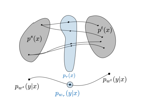
Figure 1: Coupled transfer of the data and the conditional distribution. We solve an optimization problem that transports the source data distribution ${p_{s}}(x)$ to the target distribution ${p_{t}}(x)$ as $\tau\to 1$ while simultaneously updating the model using samples from the interpolated distribution ${p_{\tau}}(x)$. This modifies the conditional distribution $p_{w_{s}}(y|x)$ on the source task to the corresponding distribution on the target task $p_{w_{t}}(y|x)$. The “coupled transfer distance” between source and target tasks is the length of the shortest such weight trajectory under the Fisher Information Metric.

Desiderata. Our desiderata for a task distance are as follows. First, it should be a distance between learning tasks, i.e., it should explicitly incorporate the hypothesis space of the model that is being transferred and accurately reflect the difficulty of transfer. For example, it is often observed in practice that transferring larger models is easier, we would like our task distance to capture this fact. Such a distance is different than discrepancy measures on the input, or the joint input-output space, which do not consider the model.

Second, we would like a theoretical framework to prescribe this distance. Task distances in the literature often depend upon quantities such as the number of epochs of fine-tuning to reach a certain accuracy, where different hyper-parameters may result in different conclusions. Also, as the present paper explores at depth, there are mechanisms for transfer other than fine-tuning that may transfer easily across tasks that are considered far away for fine-tuning.

Contributions. We formalize a “coupled transfer distance” between learning tasks as the length of the shortest trajectory on a Riemannian manifold (statistical manifold of parametrized conditional distributions of labels given data) that the weights of a classifier travel on when they are adapted from the source task to the target task. At each instant during this transfer, weighs are fitted on a interpolating task that evolves along the optimal transportation (OT) trajectory between source and target tasks. Evolution of weights and the interpolated task is coupled together. In particular, we set the ground metric which defines the cost of transporting unit mass in OT to be the Fisher-Rao distance.

We give an algorithm to compute the coupled transfer distance. It alternately update the OT map and the weight trajectory; the former uses the latest ground metric computed as the length of the weight trajectory under the Fisher Information Metric (FIM) whereas the weight trajectory is updated to fit to a new sequence of interpolated tasks given by the updated OT. We develop several techniques to scale up this algorithm and show that we can compute the coupled transfer distance between standard benchmark datasets.

We study this distance using Rademacher complexity. We show that given an OT between tasks, the Fisher-Rao distance between the initial and final weights, which our coupled transfer distance computes, corresponds to finding a weight trajectory that keeps the generalization gap small on the interpolated tasks. The coupled transfer distance thus captures the intuitive idea that a good transfer trajectory is the one that keeps the generalization gap small during transfer, in particular at the end on the target task.

We perform thorough empirical validation and analysis of the coupled transfer distance across diverse image classification datasets (MNIST (LeCun et al., 1998), CIFAR-10, CIFAR-100 (Krizhevsky & Hinton, 2009) and Deep Fashion (Liu et al., 2016)).

2 Theoretical setup

We are interested in the supervised learning problem in this paper. Consider a source dataset ${D_{s}}=\left\{(x_{s}^{i},y_{s}^{i})\right\}_{i=1}^{{N_{s}}}$ and a target dataset ${D_{t}}=\left\{(x_{t}^{i},y_{t}^{i})\right\}_{i=1}^{{N_{t}}}$ where $x_{s}^{i},x_{t}^{i}\in X$ denote input data and $y_{s}^{i},y_{t}^{i}\in Y$ denote ground-truth annotations. Training a parameterized classifier, say a deep network with weights $w\in\mathbb{R}^{p}$, on the source task involves minimizing the cross-entropy loss $\ell_{s}(w)=-\frac{1}{{N_{s}}}\sum_{i=1}^{N_{s}}\log p_{w}(y_{s}^{i}|x_{s}^{i})$ using stochastic gradient descent (SGD):

$$w(\tau+\text{d}\tau)=w(\tau)-\hat{\operatorname{\nabla}}\ell_{s}(w(\tau))\ \text{d}\tau;\ w(0)={w_{s}};$$ (1)

The notation $\widehat{\operatorname{\nabla}}\ell_{s}(w)$ indicates a stochastic estimate of the gradient using a mini-batch of data. The parameter $\text{d}\tau$ is the learning rate. Let us define the distribution $\hat{p}_{s}(x,y)=\frac{1}{{N_{s}}}\sum_{i=1}^{N_{s}}\delta_{x_{s}^{i}}(x)\delta_{y_{s}^{i}}(y)$ and its input-marginal $\hat{p}_{s}(x)=\frac{1}{{N_{s}}}\sum_{i=1}^{N_{s}}\delta_{x_{s}^{i}}(x)$; distributions $\hat{p}_{t}(x,y),\hat{p}_{t}(x)$ are defined analogously.

2.1 Fisher-Rao metric on the manifold of probability distributions

Consider a manifold $\mathcal{M}=\left\{p_{w}(z):w\in\mathbb{R}^{p}\right\}$ of probability distributions. Information Geometry (Amari, 2016) studies invariant geometrical structures on such manifolds. For two points $w,w^{\prime}\in\mathcal{M}$, we can use the Kullback-Leibler (KL) divergence $\text{KL}\left[p_{w},p_{w^{\prime}}\right]=\int\text{d}p_{w}(z)\log\left(p_{w}(z)/p_{w^{\prime}}(z)\right),$ to obtain a Riemannian structure on $M$. This allows the infinitesimal distance $\text{d}s$ on the manifold to be written as

$$\text{d}s^{2}=2\text{KL}\left[p_{w},p_{w+\text{d}w}\right]=\sum_{i,j=1}^{p}g_{ij}\ \text{d}w_{i}\text{d}w_{j}$$ (2)

$$g_{ij}(w)=\int\text{d}p_{w}(z)\left(\partial_{w_{i}}\log p_{w}(z)\right)\left(\partial_{w_{j}}\log p_{w}(z)\right)$$ (3)

are elements of the Fisher Information Matrix (FIM) $g$. Weights $w$ play the role of a coordinate system for computing the distance. The FIM is the Hessian of the KL-divergence; we may think of the FIM as quantifying the amount of information present in the model about the data it was trained on. The FIM is the unique metric on $\mathcal{M}$ (up to scaling) that is preserved under diffeomorphisms (Bauer et al., 2016), in particular under representation of the model.

Given a continuously differentiable curve $\left\{w(\tau)\right\}_{\tau\in[0,1]}$ on the manifold $M$ we can compute its length by integrating the infinitesimal distance $\left|\text{d}s\right|$ along it. The shortest length curve between two points $w,w^{\prime}\in\mathcal{M}$ induces a metric on $\mathcal{M}$ known as the Fisher-Rao distance (Rao, 1945)

$$\scalebox{0.9}{\mbox{$\displaystyle d_{\text{FR}}(w,w^{\prime})=\min_{\begin{subarray}{c}w:\ w(0)=w\\ w(1)=w^{\prime}\end{subarray}}\ \int_{0}^{1}\sqrt{\left\langle\dot{w}(\tau),g(w(\tau))\dot{w}(\tau)\right\rangle}\ \text{d}\tau$}}.$$ (4)

Shortest paths on a Riemannian manifold are geodesics, i.e., they are locally “straight lines”.

Computing the Fisher-Rao distance by integrating the KL-divergence. Let us focus on the conditional distribution $p_{w}(y|x)$. For the factorization $p(x,y)=p(x)p(y|x)$ where only the latter is parametrized, the FIM in Equation 3 is given by

$$\scalebox{0.9}{\mbox{$\displaystyle g_{ij}(w)=\operatorname*{\mathbb{E}}_{\begin{subarray}{c}x\sim p(x),\ y\sim p_{w}(y|x)\end{subarray}}\left[\partial_{w_{i}}\log p_{w}(y|x)\ \partial_{w_{j}}\log p_{w}(y|x)\right]$}};$$

here the input distribution $p(x)$ and the weights $w$ will be chosen in the following sections. The FIM is difficult to compute for large models and approximations often work poorly (Kunstner et al., 2019). For our purposes, we only need to compute the infinitesimal distance $\left|\text{d}s\right|$ in Equation 2 and can thus rewrite Equation 4 as

$$\scalebox{0.85}{\mbox{$\displaystyle d_{\text{FR}}(w,w^{\prime})=\min_{\begin{subarray}{c}w:\ w(0)=w\\ w(1)=w^{\prime}\end{subarray}}\ \int_{0}^{1}\sqrt{2\text{KL}[p_{w}(y|x),p_{w+\text{d}w}(y|x)]}$}}.$$ (5)

2.2 Transporting the data distribution

We next focus on the marginals on the input data $\hat{p}_{s}(x)$ and $\hat{p}_{t}(x)$ for the source and target tasks respectively. We are interested in computing a distance between the source marginal and the target marginal and will use tools from optimal transportation (OT) for this purpose; see Santambrogio (2015); Peyré & Cuturi (2019) for an elaborate treatment.

OT for continuous measures. Let $\Pi({p_{s}},{p_{t}})$ be the set of joint distributions (also known as couplings or transport plans) with first marginal equal to ${p_{s}}(x)$ and second marginal ${p_{t}}(x)$. The Kantorovich relaxation of OT solves for

$$\inf_{\gamma\in\Pi({p_{s}},{p_{t}})}\int c(x,x^{\prime})\ \text{d}\gamma(x,x^{\prime})$$

to compute the best coupling $\gamma^{*}\in\Pi$. The cost $c(x,x^{\prime})\in\mathbb{R}_{+}$ is called the ground metric. It gives the cost of transporting unit mass from $x$ to $x^{\prime}$. The popular squared-Wasserstein metric $W^{2}_{2}({p_{s}},{p_{t}})$ uses $c(x,x^{\prime})=\lVert x-x^{\prime}\rVert_{2}^{2}$. Given the optimal coupling $\gamma^{*}$, we can compute the trajectory that transports probability mass using displacement interpolation (mccannConvexityPrincipleInteracting1997). For example, for the Wasserstein metric, $\gamma^{*}$ is a constant-speed geodesic, i.e., if ${p_{\tau}}$ is the distribution at an intermediate time instant $\tau\in[0,1]$ then its distance from ${p_{s}}$ is proportional to $\tau$

$$W_{2}({p_{s}},{p_{\tau}})=\tau W_{2}({p_{s}},{p_{t}}).$$

OT for discrete measures. We are interested in computing the constant-speed geodesic for discrete measures $\hat{p}_{s}(x)$ and $\hat{p}_{t}(x)$. The set of transport plans in this case is $\Pi(\hat{p}_{s},\hat{p}_{t})=\left\{\Gamma\in\mathbb{R}^{{N_{s}}\times{N_{t}}}_{+}:\ \Gamma\mathbbm{1}_{N_{s}}=\hat{p}_{s},\Gamma^{\top}\mathbbm{1}_{N_{t}}=\hat{p}_{t}\right\}$ and the optimal coupling is given by

$$\Gamma^{*}=\operatorname*{\text{argmin}}_{\Gamma\in\Pi(\hat{p}_{s},\hat{p}_{t})}\left\{\left\langle\Gamma,C\right\rangle-\epsilon H(\Gamma)\right\};$$ (6)

here $C_{ij}$ is a matrix that defines the ground metric in OT. For instance, $C_{ij}=\lVert x_{i}-x^{\prime}_{j}\rVert_{2}^{2}$ for the Wasserstein metric. The first term above measures the total cost $\sum_{ij}\Gamma_{ij}C_{ij}$ incurred for the transport. The second term is an entropic penalty $H(\Gamma)=-\sum_{ij}\Gamma_{ij}\log\Gamma_{ij}$ popularized by Cuturi (2013) that accelerates the solution of the OT problem. McCann’s interpolation for the discrete case with $C_{ij}=\lVert x_{s}^{i}-x_{t}^{j}\rVert_{2}^{2}$ can be written explicitly as a sum of Dirac-delta distributions supported at interpolated inputs $x=(1-\tau)x_{s}^{i}+\tau x_{t}^{j}$

$${\hat{p}_{\tau}}(x)=\sum_{i=1}^{N_{s}}\sum_{j=1}^{N_{t}}\Gamma^{*}_{ij}\ \delta_{(1-\tau)x_{s}^{i}+\tau x_{t}^{j}}(x).$$ (7)

We can also create pseudo labels for samples from ${p_{\tau}}$ by a linear interpolation of the one-hot encoding of their respective labels to get

$$\scalebox{0.85}{\mbox{$\displaystyle{\hat{p}_{\tau}}(x,y)=\sum_{i=1}^{N_{s}}\sum_{j=1}^{N_{t}}\Gamma^{*}_{ij}\ \delta_{(1-\tau)x_{s}^{i}+\tau x_{t}^{j}}(x)\ \delta_{(1-\tau)y_{s}^{i}+\tau y_{t}^{j}}(y)$}}.$$ (8)

3 Coupled Transfer Distance

We next combine the development of Sections 2.1 to 2.2 to transport the marginal on the data and modify the weights on the statistical manifold simultaneously. We call this method the “coupled transfer process” and the corresponding task distance as the “coupled transfer distance”. We also discusses techniques to efficiently implement the process and make it scalable to large deep networks.

3.1 Uncoupled Transfer Distance

We first discuss a simple transport mechanism instead of OT and discuss how to compute a transfer distance. For $\tau\in[0,1]$, consider the mixture distribution

$${\hat{p}_{\tau}}(x,y)=(1-\tau)\hat{p}_{s}(x,y)+\tau\hat{p}_{t}(x,y).$$ (9)

Samples from ${\hat{p}_{\tau}}$ can be drawn by sampling an input-output pair from $\hat{p}_{s}$ with probability $1-\tau$ and sampling it from $\hat{p}_{t}$ otherwise. At each time instant $\tau$, the uncoupled transfer process updates the weights the classifier using SGD to fit samples from ${\hat{p}_{\tau}}$

$$w(\tau+\text{d}\tau)=w(\tau)-\hat{\operatorname{\nabla}}\ell_{\tau}(w(\tau))\ \text{d}\tau;\ w(0)={w_{s}}.$$ (10)

Weights $w(\tau)$ are thus fitted to each task ${p_{\tau}}$ as $\tau$ goes from 0 to 1. In particular for $\tau=1$, weights $w(1)$ are fitted to $\hat{p}_{t}$. As $\text{d}\tau\to 0$, we obtain a continuous curve $\left\{w(\tau):t\in[0,1]\right\}$. Computing the length of this weight trajectory using Equation 5 gives a transfer distance.

Remark 1 (Uncoupled transfer distance entails longer weight trajectories).

For uncoupled transfer, although the task and weights are modified simultaneously, their changes are not synchronized. We therefore call this the “uncoupled transfer distance”. To elucidate, changes in the data using the mixture Equation 9 may be unfavorable to the current weights $w(\tau)$ and may cause the model to struggle to track the distribution ${\hat{p}_{\tau}}$. This forces the weights to take a longer trajectory in information space, i.e., as measured by the Fisher-Rao distance in Equation 5. If changes in data were synchronized with the evolving weights, the weight trajectory would be necessarily shorter in information space because the KL-divergence in Equation 2 is large when the conditional distribution changes quickly to track the evolving data. We therefore expect the task distance computed using the mixture distribution to be larger than the coupled transfer distance which we will discuss next; our experiments in Section 5 corroborate this.

3.2 Modifying the task and classifier synchronously

Our coupled transfer distance that uses OT to modify the task and updates the weights synchronously to track the interpolated distribution is defined as follows.

Definition 2 (Coupled transfer distance).

Given two learning tasks ${D_{s}}$ and ${D_{t}}$ and a $w$-parametrized classifier trained on ${D_{s}}$ with weights ${w_{s}}$, the coupled transfer distance between the tasks is

where and couplings $\Gamma\in\Pi(\hat{p}_{s}(x),\hat{p}_{t}(x))$ and $w(\cdot)$ is a continuous curve which is the limit of

$$w(\tau+\text{d}\tau)=w(\tau)-\hat{\operatorname{\nabla}}\ell_{\tau}(w(\tau))\ \text{d}\tau;\ w(0)={w_{s}}.$$

as $\text{d}\tau\to 0$. The interpolated distribution $\hat{p}_{\tau}(x,y)$ at time instant $\tau\in[0,1]$ for a coupling $\Gamma$ is given by Equation 8 and the loss $\ell_{\tau}$ is the cross-entropy loss of fitting data from this interpolated distribution.

The following remarks discuss the rationale and the properties of this definition.

Remark 3 (Coupled transfer distance is asymmetric).

The length of the weight trajectory for transferring from $\hat{p}_{s}$ to $\hat{p}_{t}$ is different from the one that transfers from $\hat{p}_{t}$ to $\hat{p}_{s}$. This is a desirable property, e.g., it is easier to transfer from ImageNet to CIFAR-10 than in the opposite direction.

Remark 4 (Coupled transfer distance can be compared across different architectures).

An important property of the task distance in Equation 11 is that it is the Fisher-Rao distance, i.e., the shortest geodesic on the statistical manifold, of conditional distributions $p_{w(0)}(\cdot|x_{s}^{i})$ and $p_{w(1)}(\cdot|x_{t}^{i})$ with the coupling $\Gamma$ determining the probability mass that is transported from $x_{s}^{i}$ to $x_{t}^{j}$. Since the Fisher-Rao distance, does not depend on the embedding dimension of the manifold $M$, the coupled transfer distance does not depend on the architecture of the classifier; it only depends upon the capacity to fit the conditional distribution $p_{w}(y|x)$. This is a very desirable property: given the tasks, our distance is comparable across different architectures. Let us note that the uncoupled transfer distance in Section 3.1 also shares this property but coupled transfer has the benefit of computing the shortest trajectory in information space; weight trajectories of uncoupled transfer may be larger; see Remark 1.

3.3 Computing the coupled transfer distance

We first provide an an informal description of how we compute the task distance. Each entry $\Gamma_{ij}$ of the coupling matrix determines how much probability mass from $x_{s}^{i}$ is transported to $x_{t}^{j}$. The interpolated distribution Equation 8 allows us to draw samples from the task at an intermediate instant. For each coupling $\Gamma$, there exists a trajectory of weights $w(\cdot):=\left\{w(\tau):\tau\in[0,1]\right\}$ that tracks the interpolated task. The algorithm treats $\Gamma$ and the weight trajectory as the two variables and updates them alternately as follows. At the $k^{\text{th}}$ iteration, given a weight trajectory $w^{k}(\cdot)$ and a coupling $\Gamma^{k}$, we set the entries of the ground metric $C^{k+1}_{ij}$ to be the Fisher-Rao distance between distributions $p_{w(0)}(\cdot|x_{s}^{i})$ and $p_{w(1)}(\cdot|x_{t}^{i})$. An updated $\Gamma^{k+1}$ is calculated using this ground metric to result in a new trajectory $w^{k+1}(\cdot)$ that tracks the new interpolated task distribution Equation 8 for $\Gamma^{k+1}$.

More formally, given an initialization for the coupling matrix $\Gamma^{0}$ we perform the updates in Equation 12. Computing the coupled transfer distance is a non-convex optimization problem and we therefore include a proximal term in Equation 12a to keep the coupling matrix close to the one computed in the previous step $\Gamma^{k}$. This also indirectly keeps the weight trajectory $w^{k+1}(\cdot)$ close to the trajectory from the previous iteration. Proximal point iteration (Bauschke & Combettes, 2017) is insensitive to the step-size $\lambda$ and it is therefore beneficial to employ it in these updates.

$$\scalebox{0.9}{\mbox{$\displaystyle\Gamma^{k}=\operatorname*{\text{argmin}}_{\Gamma\in\Pi}\left\{\left\langle\Gamma,C^{k}\right\rangle-\epsilon H(\Gamma)+\lambda\lVert\Gamma-\Gamma^{k-1}\rVert_{\text{F}}^{2}\right\}$}},$$ (12a)

$$\scalebox{0.9}{\mbox{$\displaystyle C^{k}_{ij}=\int_{0}^{1}\sqrt{2\text{KL}\left[p_{{w^{k}(\tau)}}(\cdot|x_{\tau}^{ij}),p_{{w^{k}(\tau+\text{d}\tau)}}(\cdot|x_{\tau}^{ij})\right]}$}},$$ (12b)

(12c)

$$\scalebox{0.8}{\mbox{$\displaystyle{\hat{p}_{\tau}}(x,y)=\sum_{i=1}^{N_{s}}\sum_{j=1}^{N_{t}}\Gamma^{k-1}_{ij}\ \delta_{(1-\tau)x_{s}^{i}+\tau x_{t}^{j}}(x)\ \delta_{(1-\tau)y_{s}^{i}+\tau y_{t}^{j}}(y)$}},$$ (12d)

$$x_{\tau}^{ij},y_{\tau}^{ij}\sim{\hat{p}_{\tau}}(x,y).$$ (12e)

3.4 Practical tricks for efficient computation

The optimization problem formulated in Equation 12 is conceptually simple but computationally daunting. The main hurdle is to compute the ground metric $C^{k}_{ij}$ for all $i\leq{N_{s}},j\leq{N_{t}}$ pairs in a dense transport coupling $\Gamma$. The coupling matrix can be quite large, e.g., it has $10^{8}$ entries for a relatively small dataset of ${N_{s}}={N_{t}}=10,000$. We therefore introduce the following techniques that allow us to scale to large problems.

Block-diagonal transport couplings. Instead of optimizing $\Gamma$ in Equation 11 over the entire polytope $\Pi(\hat{p}_{s},\hat{p}_{t})$, we only consider block-diagonal couplings. Depending upon the source and target datasets, we use blocks of size up to 30$\times$30. At each time instant $\tau\in[0,1]$, we sample a block from the transport coupling. SGD in Equation 12c updates weights using multiple samples from the interpolated task restricted to this block. The integrand for $C^{k}_{ij}$ in Equation 12b is also computed only on this mini-batch. Experiments in Section 5 show that the weight trajectory converges using this technique. We can compute the coupling transfer distance for source and target datasets of size up to ${N_{s}}={N_{t}}=19,200$. Other approaches for handling large-scale OT problems such as hierarchical methods (Lee et al., 2019) or greedy computation (Carlier et al., 2010) could also be used for our purpose but we chose this one for sake of simplicity.

Initializing the transport coupling. The ground metric $C_{ij}=\lVert x_{s}^{i}-x_{t}^{j}\rVert_{2}^{2}$ is widely used in the OT literature. We are however interested in computing distances for image-classification datasets in this paper and such a pixel-wise distance is not a reasonable ground metric for visual data that have strong local/multi-scale correlations. We therefore set $\Gamma^{0}$ to be the block-diagonal approximation of the transport coupling for the ground metric $C_{ij}=\lVert\varphi(x_{s}^{i})-\varphi(x_{t}^{j})\rVert_{2}^{2}$ where $\varphi$ is some feature extractor. The feature space is much more Euclidean-like than the input space and this gives us a good initialization in practice; similar ideas are employed in the metric learning literature (Snell et al., 2017; Hu et al., 2015; Qi et al., 2018). We use a ResNet-50 (He et al., 2016) pre-trained on ImageNet to initialize $\Gamma^{0}$ for all our experiments. To emphasize, we use the feature extractor only for initializing the transport coupling further updates are performed using Equation 12a. We have computed the coupling transfer distance for MNIST without this step and our results are similar.

Using mixup to interpolate source and target images. The interpolating distribution Equation 8 has a peculiar nature: sampled data $x_{\tau}^{ij}=(1-\tau)x_{s}^{i}+\tau x_{t}^{j}$ from this distribution are a convex combination of source and target data. This causes artifacts for natural images for $\tau$ away from 0 or 1; we diagnosed this as a large value of the training loss while executing Equation 10. We therefore treat the coefficient of the convex combination in Equation 8 as if it were a sample from a Beta-distribution $\text{Beta}(\tau,1-\tau)$. This keeps the samples $x_{\tau}^{ij}$ similar to the source or the target task and avoids visual artifacts. This trick is inspired by Mixup regularization  (Zhang et al., 2017); we also use Mixup for labels $y_{\tau}^{ij}$.

4 An alternative perspective using Rademacher complexity

We have hitherto motivated the coupled transfer distance using ideas in information geometry. In this section, we study the weight trajectory under the lens of learning theory. We show that we can interpret it as the trajectory that minimizes the integral of the generalization gap as the the weights are adapted from the source to the target task. We consider binary classification tasks in this section. Rademacher complexity (Bartlett & Mendelson, 2001)

$$\scalebox{0.9}{\mbox{$\displaystyle\mathcal{R}_{N}(r)=\operatorname*{\mathbb{E}}_{\hat{p}\sim p}\left[\operatorname*{\mathbb{E}}_{\sigma}\left[\sup_{w\in A(r)}\frac{1}{N}\sum_{i=1}^{N}\ \sigma^{i}\ell(w;x^{i},y^{i})\right]\right]$}},$$ (13)

is the average over draws of the dataset $\hat{p}\sim p$ and iid random variables $\sigma^{i}$ uniformly distributed over $\left\{-1,1\right\}$ of the worst case average weighted loss $\sigma^{i}\ell(w;x^{i},y^{i})$ for $w$ in the set $A(r)$. We assume here that $\left|\ell(w;x^{i},y^{i})\right|<M$ and $\ell(w;x,y)$ is Lipschitz continuous. Classical bounds bound the generalization gap of all hypotheses $h$ in a hypothesis class $\mathcal{H}$ by $\mathcal{R}_{2N}(\mathcal{H})+2\sqrt{\frac{\log(1/\delta)}{N}}$ with probability at least $1-\delta$. We build upon this result to get the following theorem under the assumption that weights $w(\tau)$ predict well on the interpolated task ${\hat{p}_{\tau}}(x,y)$ at all times $\tau$.

Theorem 5.

Given a weight trajectory $\left\{{w(\tau)}\right\}_{\tau\in[0,1]}$ and a sequence $0=\tau_{0}\leq\tau_{1}<\tau_{2}<...<\tau_{K}\leq 1$, for all $\epsilon>2\sum_{k=1}^{K}(\tau_{k}-\tau_{k-1})\operatorname*{\mathbb{E}}_{x\sim p_{\tau}}|\Delta\ell(w(\tau_{k-1}))|$, the probability that

is greater than $\epsilon$ is upper bounded by

$$\scalebox{0.8}{\mbox{$\displaystyle\exp\left\{-\frac{2K}{M^{2}}\left(\epsilon-2\sum_{k=1}^{K}\Delta\tau_{k}\operatorname*{\mathbb{E}}_{x\sim p_{\tau_{k}}}\left[\sqrt{\left\langle\dot{w}(\tau_{k}),g(w(\tau_{k}))\dot{w}(\tau_{k})\right\rangle}\right]\right)\right\}$}}.$$ (14)

We have defined $\Delta\tau_{k}=\tau_{k}-\tau_{k-1}$ and $\Delta\ell({w(\tau)})=\ell({w(\tau+\text{d}\tau)};x,y_{\tau}(x))-\ell({w(\tau)};x,y_{\tau}(x))$.

Appendix C gives the proof. As $\Delta\tau_{k}\to 0$

which is the length of the trajectory on the statistical manifold with inputs drawn from the interpolated distribution at each instant.

We can thus think of the coupled transfer distance as the length of the trajectory on the statistical manifold that starts at the given model ${w_{s}}$ on the source task and ends with the model $w(1)$ fitted to the target task, as the task is simultaneously interpolated using an optimal transport whose ground metric between samples $x_{s}^{i}$ and $x_{t}^{j}$ is $C_{ij}=\int_{0}^{1}\sqrt{2\text{KL}\left[p_{w(\tau)}(\cdot|x_{\tau}^{ij}),p_{w(\tau+\text{d}\tau)}(\cdot|x_{\tau}^{ij})\right]}$ which is the length of the trajectory under the FIM. This result is a crisp theoretical characterization of the intuitive idea that if one finds a weight trajectory that transfers from the source to the target task while keeping the generalization gap small at all time instants, then the length of the trajectory is a good indicator of the distance between tasks.

5 Experiments

5.1 Setup

We use the MNIST, CIFAR-10, CIFAR-100 and Deep Fashion datasets for our experiments. Source and target tasks consist of subsets of these datasets, each task with one or more of the original classes inside it. We show results using an 8-layer convolutional neural network with ReLU nonlinearities, dropout, batch-normalization with a final fully-connected layer along with a larger wide-residual-network WRN-16-4 (Zagoruyko & Komodakis, 2016).  Appendix A gives details about pre-processing, architecture and training.

5.2 Baseline methods to estimate task distances

The difficulty of fine-tuning is the gold standard of distance between tasks. It is therefore very popular, e.g., Kornblith et al. (2019) use the number of epochs during transfer as the distance. We compute the length of the weight trajectory, i.e., $\int_{0}^{1}\left|\text{d}w\right|$ and call this the fine-tuning distance. The trajectory is truncated when validation accuracy on the target task is 95% of its final validation accuracy. No transport of the task is performed and the model directly takes SGD updates on the target task after being pre-trained on the source task.

The next baseline is Task2Vec (Achille et al., 2019a) which embeds tasks using the diagonal of the FIM of a model trained on them individually. Cosine distance between these vectors is defined as the task distance.

We also compare with the uncoupled transfer distance developed in Section 3.1. This distance computes length of the weight trajectory on the Riemannian distance and also interpolates the data but does not do them synchronously.

Discrepancy measures on the input space are a popular way to measure task distance. We show task distance computed as the Wasserstein $W_{2}^{2}$ metric on the the pixel-space, the Wasserstein $W_{2}^{2}$ metric on the embedding space and also method that we devised ourselves where we transfer a variational autoencoder (VAE (Kingma & Welling, 2014)) from the source to the target task and compute the length of weight trajectory on the manifold. We transfer the VAE in two ways, (i) by directly fitting the model on the target task, and (ii) by interpolating the task using a mixture distribution as described in Section 3.1.

5.3 Quantitative comparison of distance matrices

Metrics are not unique. We would however still like to compare two task distances across various pairs of tasks. In addition to showing these matrices and drawing qualitative interpretations, we use the Mantel test (Mantel, 1967) to accept/reject the null hypothesis that variations in two distance matrices are correlated. We will always compute correlations with the fine-tuning distance matrix because it is a practically relevant quantity and task distances are often designed to predict this quantity. We report $p$-values and the normalized test statistic $r=1/(n^{2}-n-1)\sum_{i,j=1}^{n}(a_{ij}-\bar{a})(b_{ij}-\bar{b})/(\sigma_{a}\sigma_{b})$ where $a,b\in\mathbb{R}^{n\times n}$ are distance matrices for $n$ tasks, $\bar{a},\sigma_{a}$ denote mean and standard deviation of entries respectively. Numerical values of $r$ are usually small for all data (Ape, ; Goslee et al., 2007) but the pair $(r,p)$ are a statistically sound way of comparing distance matrices; large $r$ with small $p$ indicates better correlation.

5.4 Transferring between subsets of benchmark datasets

CIFAR-10 and CIFAR-100. We consider four tasks (i) all vehicles (airplane, automobile, ship, truck) in CIFAR-10, (ii) the remainder, namely six animals in CIFAR-10, (iii) the entire CIFAR-10 dataset and (iv) the entire CIFAR-100 dataset. We show results in Figure 2 using 4$\times$4 distance matrices where numbers in each cell indicate the distance between the source task (row) and the target task (column).

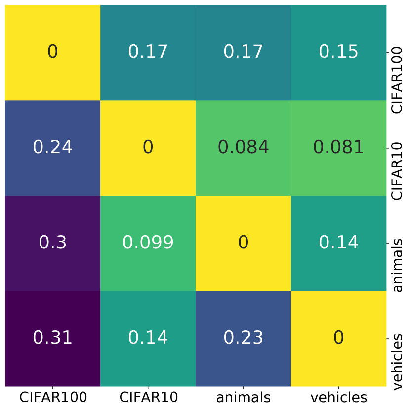
(a)

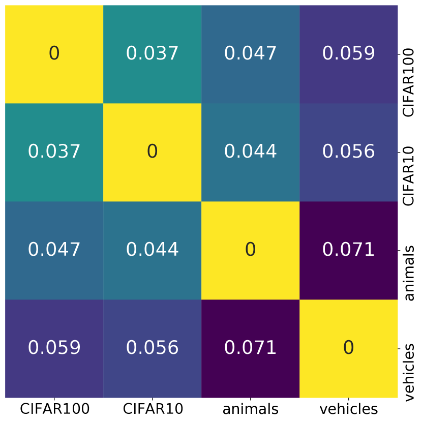
(b)

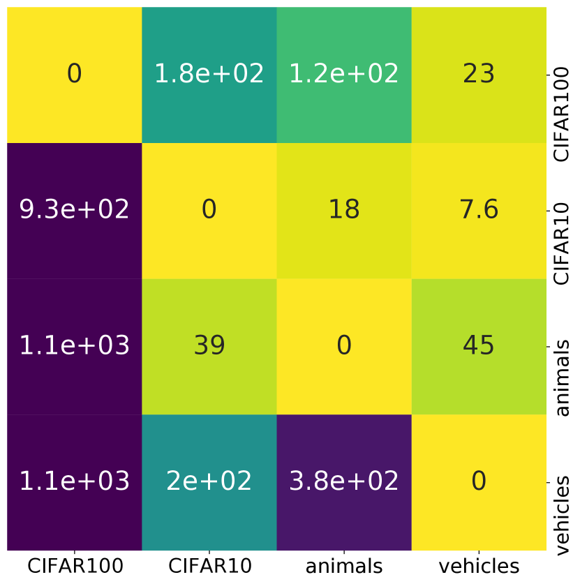
(c)

Figure 2: Figure 2(a) shows coupled transfer distance ($r$ = 0.428 $p$ = 0.13), Figure 2(b) shows distances estimated using Task2Vec ($r$ = 0.03, $p$ = 0.98), Figure 2(c) shows fine-tuning distance ($r$ = 0.61, $p$ = 0.09 with itself). The numerical values of the distances in this figure are not comparable with each other. Coupled transfer distances satisfy certain sanity checks, e.g., transferring to a subset task is easier than transferring from a subset task (CIFAR-10-vehicles/animals), which Task2Vec does not.

Coupled transfer shows similar trends as fine-tuning, e.g., the tasks animals-CIFAR-10 or vehicles-CIFAR-10 are close to each other while CIFAR-100 is far away from all tasks (it is closer to CIFAR-10 than others). Task distance is asymmetric in Figure 2(a), Figure 2(c). Distance from CIFAR-10-animals is smaller than animals-CIFAR-10; this is expected because animals is a subset of CIFAR-10. Task2Vec distance estimates in Figure 2(b) are qualitatively quite different from these two; the distance matrix is symmetric. Also, while fine-tuning from animals-vehicles is relatively easy, Task2Vec estimates the distance between them to be the largest.

This experiment also shows that our approach can scale to medium-scale datasets and can handle situations when the source and target task have different number of classes.

Transferring between subsets of CIFAR-100. We construct five tasks (herbivores, carnivores, vehicles-1, vehicles-2 and flowers) that are subsets of the CIFAR-100 dataset. Each of these tasks consists of 5 sub-classes. The distance matrices for coupled transfer, Task2Vec and fine-tuning are shown in Figure 3(a), Figure 3(b) and Figure 3(c) respectively. We also show results using uncoupled transfer in Figure 3(d).

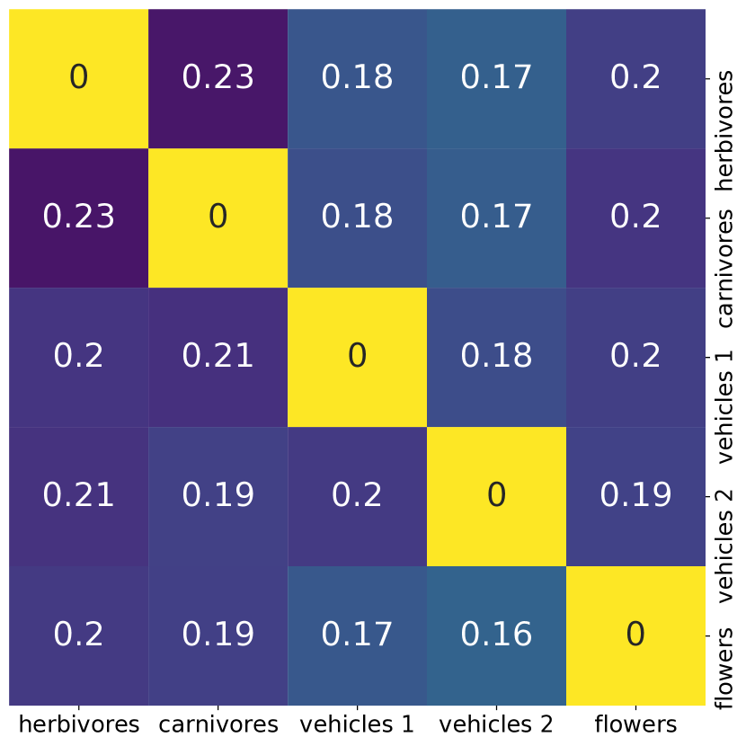
(a)

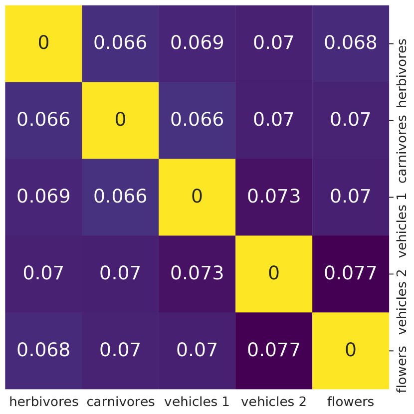
(b)

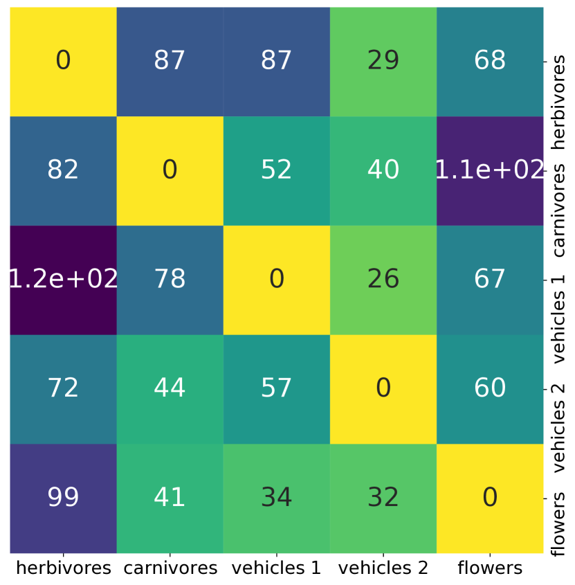
(c)

(d)

Figure 3: Figure 3(a) shows coupled transfer distance ($r$ = 0.14, $p$ = 0.05), Figure 3(b) shows Task2Vec distance ($r$ = 0.07, $p$ = 0.17), Figure 3(c) shows fine-tuning distance ($r$ = 0.36, $p$ = 0.03), and Figure 3(d) shows uncoupled transfer distance ($r$ = 0.12, $p$ = 0.47). Numerical values in the first and the last sub-plot can be compared directly. Coupled transfer broadly agrees with fine-tuning except for carnivores-flowers and herbivores-vehicles-1. For all tasks, uncoupled transfer overestimates the distances compared to Figure 3(a).

Coupled transfer estimates that all these subsets of CIFAR-100 are roughly equally far away from each other with herbivores-carnivores being the farthest apart while vehicles-1-vehicles-2 being closest. This ordering is consistent with the fine-tuning distance although fine-tuning results in an extremely large value for carnivores-flowers and vehicles-1-herbivores. This ordering is mildly inconsistent with the distances reported by Task2Vec in Figure 3(b) the distance for vehicles-1-vehicles-2 is the highest here. Broadly, Task2Vec also results in a distance matrix that suggests that all tasks are equally far away from each other. As has been reported before (Li et al., 2020), this experiment also demonstrates the fragility of fine-tuning.

Recall that distances for uncoupled transfer in Figure 3(d) can be compared directly to those in Figure 3(a) for coupled transfer. Task distances for the former are always larger. Further, distance estimates of uncoupled transfer do not bear much resemblance with those of fine-tuning; see for example the distances for vehicles-2-carnivores, flowers-carnivores, and vehicles-1-vehicles-2. This demonstrates the utility of solving a coupled optimization problem in Equation 12 which finds a shorter trajectory on the statistical manifold.

Experiments on transferring between subsets of Deep Fashion are given in Appendix B. We also computed task distances for tasks with different input domains. For transferring from MNIST to CIFAR-10, the coupled transfer distance is 0.18 (0.06 in the other direction), fine-tuning distance is 554.2 (20.6 in the other direction) and Task2Vec distance is 0.149 (same in the other direction). This experiment shows that can robustly handle diverse input domains and yet again, the coupled transfer distance correlates with the fine-tuning distance .

5.5 Further analysis of the coupled transfer distance

Convergence of coupled transfer. Figure 4(a) shows the evolution of training and test loss as computed on samples of the interpolated distribution after $k=4$ iterations of Equation 12. As predicted by Theorem 5 the generalization gap is small throughout the trajectory. Training loss increases towards the middle; this is expected because the interpolated task is far away from both source and target tasks there. The interpolation Equation 12d could also be a cause for this increase.

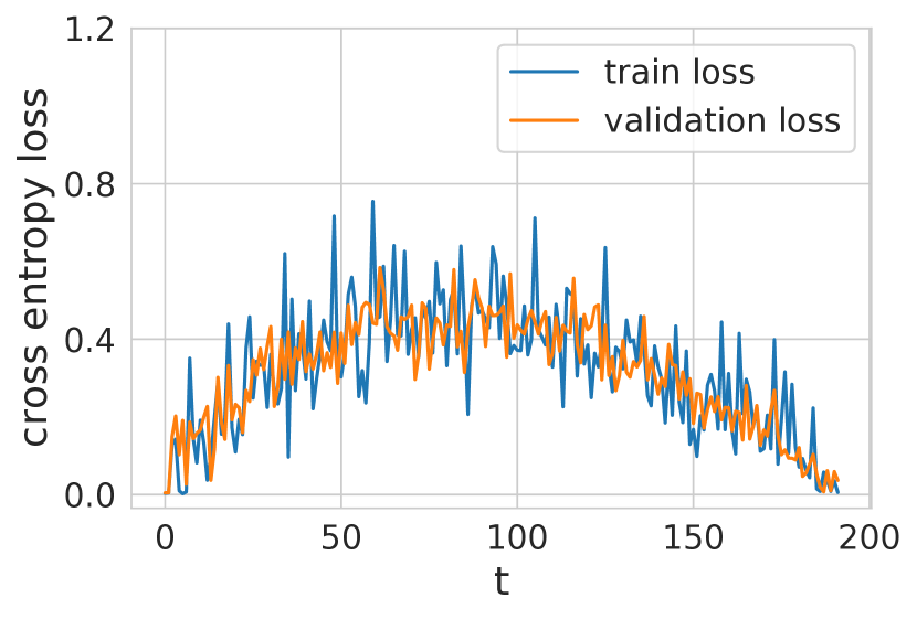
(a)

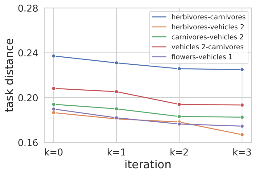
(b)

Figure 4: Figure 4(a) shows the evolution of the training and test cross-entropy loss on the interpolated distribution as a function of the transfer steps in the final iteration of coupled transfer of vehicles-1-vehicles-2. As predicted by Theorem 5, generalization gap along the trajectory is small. Figure 4(b) shows the convergence of the task distance with the number of iterations $k$ in Equation 12; the distance typically converges in 4–5 iterations for these tasks.

We typically require 4–5 iterations of Equation 12 for the task distance to converge; this is shown in Figure 4(b) for a few instances. This figure also indicates that computing the transport coupling in Equation 6 independently of the weights and using this coupling to modify the weights, as done in say (Cui et al., 2018), results in a larger distance than if one were to optimize the couplings along with the weights. The coupled transfer finds shorter trajectories for weights and will potentially lead to better accuracies on target tasks in studies like (Cui et al., 2018) because it samples more source data.

Models with a larger capacity are easier to transfer. We next show that using a model with higher capacity results in smaller distances between tasks. We consider a wide residual network (WRN-16-4) of (Zagoruyko & Komodakis, 2016) and compute distances on subsets of CIFAR-100 in Figure 5. First note that task distances for coupled transfer in Figure 5(a) are consistent with those for fine-tuning in Figure 5(b). Coupled transfer distances in  Figure 5(a) are much smaller than those in Figure 3(a).

Roughly speaking, a high-capacity model can learn a rich set of features, some discriminative and others redundant not relevant to the source task. These redundant features are useful if target task is dissimilar to the source. This experiment also demonstrates that the information-geometric distance computed by coupled transfer, which is independent of the dimension of the statistical manifold, leads to a constructive strategy for selecting architectures for transfer learning. Most methods to compute task distances instead only inform which source target is best suited to pre-train with for the target task.

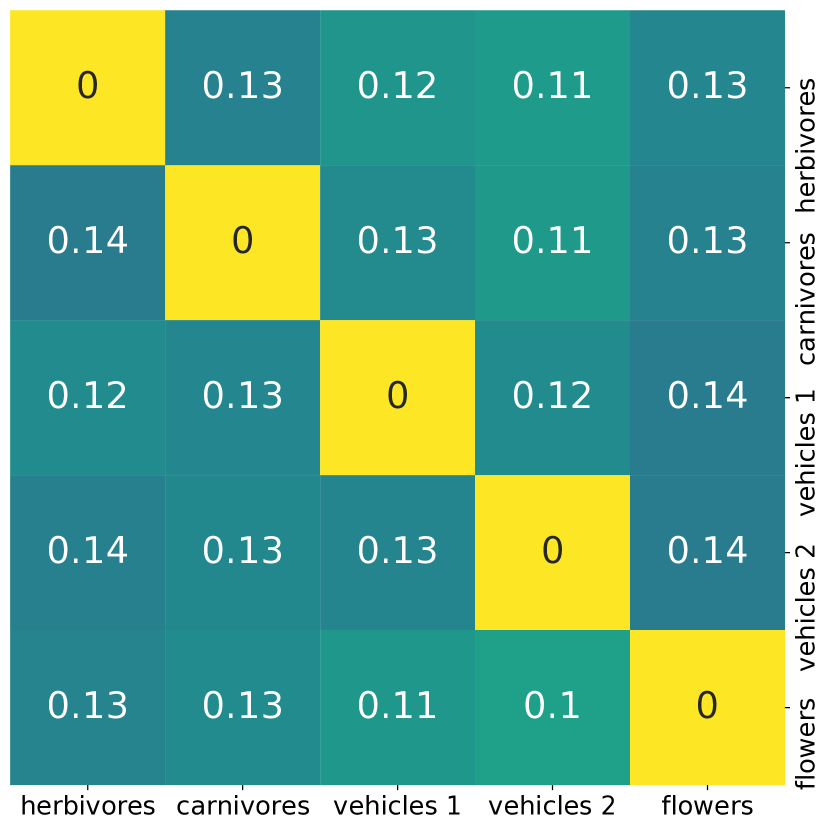
(a)

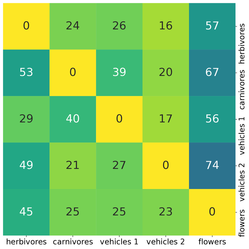
(b)

Figure 5: Figure 5(a) shows coupled transfer distance ($r$ = 0.15, $p$ = 0.01) and Figure 5(b) shows fine-tuning distance ($r$ = 0.39, $p$ = 0.01 with itself and $r$ = 0.21, $p$ = 0.20 with fine-tuning distance in Figure 3(c)). Numbers in Figure 5(a) can be directly compared to those in Figure 3(a). WRN-16-4 model has a shorter trajectory for all task pairs compared to the CNN in Figure 3(a) with fewer parameters.

Does coupled transfer lead to better generalization on the target? It is natural to ask whether the generalization performance of the model after coupled transfer is better than the one after standard fine-tuning (which does not transport the task). Figure 6 compares the validation loss and the validation accuracy after coupled transfer and after standard fine-tuning for pairs of CIFAR-100 tasks. It shows that broadly, the former improves generalization. This is consistent with existing literature (Gao & Chaudhari, 2020) which employs task interpolation for better transfer. Let us note that improving fine-tuning is not our goal while developing the task distance. In fact, we want the task distance to correlate with the difficulty of fine-tuning.

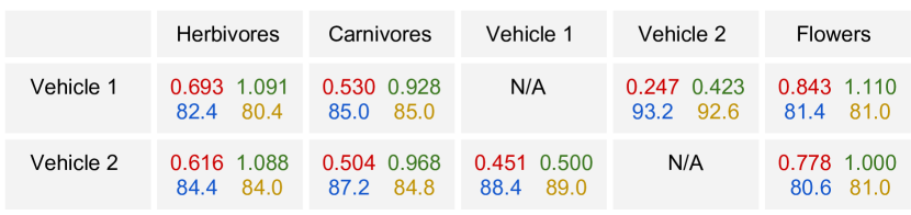
Figure 6: Comparison of validation loss (red for coupled transfer, green for fine-tuning) and accuracy (%) (blue and yellow respectively) between different subsets of CIFAR-100. Optimal transport for the task distribution results in large improvements in the validation loss in all cases; The validation accuracy also improve by 0.4%–2.5% in all cases except the last two.

Comparison with other task discrepancy measures. LABEL:{fig:vae_uncoupled} shows task distances computed using the Riemannian length of the weight trajectory for the VAE (see Section 5.2) when task is interpolated using a mixture distribution, Figure 7(b) shows the same quantity when the VAE is directly fitted to the target task after initialization on the source. Figure 7(c) and Figure 7(d) show the Wasserstein distance on the pixel-space and feature-space respectively. We find that although the four distance matrices in Figure 7 agree with each other very well ($r\approx$ 0.15, $p$ < 0.08 for all pairs, except the VAE with uncoupled transfer), they are very different from the fine-tuning distance in Figure 3(c). This shows that task distances computed using discrepancy measures on the input space are not reflective of the difficulty of fine-tuning, after all images in these tasks are visually quite similar to each each. Coupled transfer distance explicitly takes the hypothesis space into account and correctly reflects the difficulty of transfer, even if the input spaces are similar.

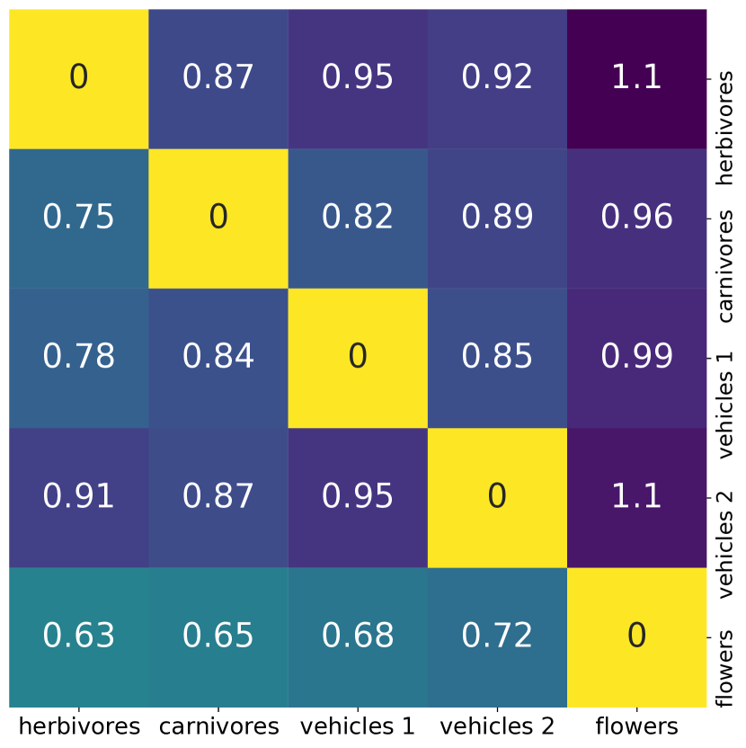
(a)

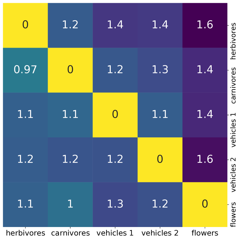
(b)

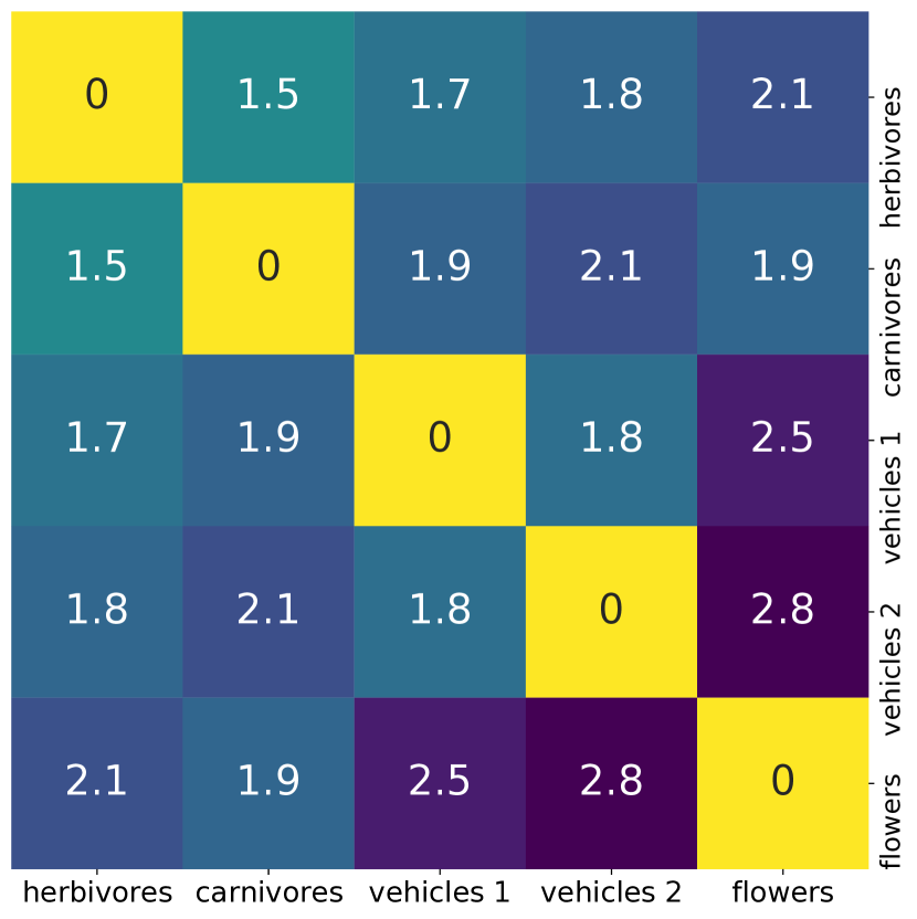
(c)

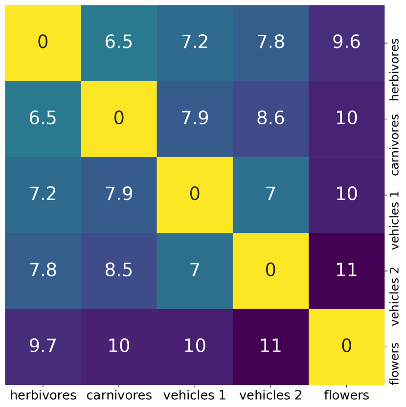
(d)

Figure 7: Figure 7(a) shows task distance computed using the Riemannian length of the weight trajectory for the VAE using a mixture distribution to interpolate the tasks (see Section 5.1, $r$ = 0.1, $p$ = 0.76), Figure 7(b) shows the same quantity for directly fine-tuning the VAE ($r$ = 0.09, $p$ = 0.88), Figure 7(c) shows task distance using the Wasserstein metric on the pixel-space ($r$ = 0.02, $p$ = 0.22), Figure 7(d) shows distances using Wasserstein metric on the embedding space ($r$ = 0.06, $p$ = 0.40). The last three methods agree with each other very well (see the narrative for $p$-values) but small Mantel test statistic and high $p$-values as compared to Figure 3(c) indicates that these distances are not correlated with the difficulty of fine-tuning.

6 Related Work

Domain-specific methods. A rich understanding of task distances has been developed in computer vision, e.g., Zamir et al. (2018) compute pairwise distances when different tasks such as classification, segmentation etc. are performed on the same input data. The goal of this work, and others such as (Cui et al., 2018), is to be able to decide which source data to pre-train to generalize well on a target task. Task distances have also been widely discussed in the multi-task learning (Caruana, 1997) and meta/continual-learning (Liu et al., 2019; Pentina & Lampert, 2014; Hsu et al., 2018). The natural language processing literature also prevents several methods to compute similarity between input data (Mikolov et al., 2013; Pennington et al., 2014).

Most of the above methods are based on evaluating the difficulty of fine-tuning, or computing the similarity in some embedding space. It is difficult to ascertain whether the distances obtained thereby are truly indicative of the difficulty of transfer; fine-tuning hyper-parameters often need to be carefully chosen (Li et al., 2020) and neither is the embedding space unique. For instance, the uncoupled transfer process that modifies the input data distribution will lead to a different estimate of task distance.

Information-theoretic approaches. We build upon a line of work that combines generative models and discriminatory classifiers (see  (Jaakkola & Haussler, 1999; Perronnin et al., 2010) to name a few) to construct a notion of similarity between input data. Modern variants of this idea include Task2Vec (Achille et al., 2019a) which embeds the task using the diagonal of the FIM and computes distance between tasks using the cosine distance for this embedding. The main hurdle in Task2Vec and similar approaches is to design the architecture for computing FIM: a small model will indicate that tasks are far away. Achille et al. (2019b, c) use the KL divergence between the posterior weight distribution and a prior to quantify the complexity of a task; distance between tasks is defined to be the increase in complexity when the target task is added to the source task. This is an elegant formalism but it is challenging to compute it accurately and it has not yet been demonstrated for a broad range of datasets.

Learning-theoretic approaches. Learning theory typically studies out-of-sample performance on a single task using complexity measures such as VC-dimension (Vapnik, 1998). These have been adapted to address the difficulty of domain adaptation (Ben-David et al., 2010; Zhang et al., 2012; Redko et al., 2019) which gives a measure of task distance that incorporates the complexity of the hypothesis space. In particular, Ben-David et al. (2010) train on a fixed mixture of the source and target data to minimize which is similar to our interpolated distribution Equation 12d. Theoretical results here corroborate (actually motivate) our experimental result that transferring between the same tasks with a higher-capacity model is easer. A key gap in this literature is that this theory does not consider how the model is adapted to target task. For complex models such as deep networks, hyper-parameters during fine-tuning play a crucial role (Li et al., 2020). Our work fundamentally exploits the idea that the task need not be fixed during transfer, it can also be adapted. Further, our coupled transfer distance is invariant to the particular parametrization of the deep network, which is difficult to achieve using classical learning theory techniques.

Coupled transfer of data and the model. Transporting the task using optimal transport is fundamental to how our coupled transfer distance is defined. This is motivated from two recent studies. Gao & Chaudhari (2020) develop an algorithm that keeps the classification loss unchanged across transfer. Their method interpolates between the source and target data using the mixture distribution from Section 3.1. We take this idea further and employ optimal transport (Cui et al., 2018) to modulate the interpolation of the task using the Fisher-Rao distance. Coupled transport problems on the input data are also solved for unsupervised translation (Alvarez-Melis & Jaakkola, 2018). The idea of modifying the task during transfer using optimal transport is also exploited by Alvarez-Melis & Fusi (2020a) to prescribe task distances and for data augmentation/interpolation and transfer (Alvarez-Melis & Fusi, 2020b).

7 Discussion

Our work is an attempt to theoretically understand when transfer is easy and when it is not. An often over-looked idea in large-scale transfer learning is that the task need not remain fixed to the target task during transfer. We heavily exploit this idea in the present paper. We develop a “coupled transfer distance” between tasks that computes the shortest weight trajectory in information space, i.e., on the statistical manifold, while the task is optimally transported from the source to the target. The most important aspect of our work is that both task and weights are modified synchronously. It is remarkable that this coupled transfer distance is not just strongly correlated with the difficulty of fine-tuning but also theoretically captures the intuitive idea that a good transfer algorithm is the one that keeps generalization gap small during transfer, in particular at the end on the target task.

Appendix A Details of the experimental setup

A.1 Architecture and training.

We show results using an 8-layer convolutional neural network with ReLU nonlinearities, dropout, batch-normalization with a final fully-connected layer. The larger model used for experiments in Figure 5 is a wide-residual-network (WRN-16-4 architecture of (Zagoruyko & Komodakis, 2016)).

A.2 Transferring between CIFAR-10 and CIFAR-100

We consider four tasks: (i) all vehicles (airplane, automobile, ship, truck) in CIFAR-10, consisting of 20,000 32$\times$32-sized RGB images; (ii) the remainder, namely six animals in CIFAR-10, consisting of 30,000 32$\times$32-sized RGB images; (iii) the entire CIFAR-10 dataset and (iv) the entire CIFAR-100 dataset, consisting of 50,000 images and spread across 100 classes.

We pre-train model on source tasks using stochastic gradient descent (SGD) for 60 epochs, with mini-batch size of 20, learning rate schedule is set to $10^{-3}$ for epochs 0 – 40 and $8\times 10^{-4}$ for epochs 40 – 60. When CIFAR-100 is the source dataset, we train for 180 epochs with the learning rate set to $10^{-3}$ for epochs 0 – 120, and $8\times 10^{-4}$ for epochs 120 – 180.

We chose a slightly smaller version of the source and target datasets to compute the distance, each of them have 19,200 images. The class distribution on all source and target classes is balanced. We did this to reduce the size of the coupling matrix $\Gamma$ in Equation 12a. The coupling matrix connecting inputs in the source and target datasets is $\Gamma\in\mathbb{R}^{19200\times 19200}$ which is still quite large to be tractable during optimization. We therefore use a block diagonal approximation of the coupling matrix; 640 blocks are constructed each of size 30$\times$30 and all other entries in the coupling matrix are set to zero at the beginning of each iteration in Equation 12a after computing the dense coupling matrix using the linear program. This effectively entails that the set of couplings over which we compute the transport is not the full convex polytope in Section 2.2 but rather a subset of it. We sample a mini-batch of 20 images from the interpolated distribution corresponding to this block-diagonal coupling matrix for each weight update of Equation 12c. We run 40 epochs, i.e., with 19200/20 = 960 weight updates per epoch for computing the weight trajectory at each iteration $k$ in Equation 12. The learning rate is fixed to $8\times 10^{-4}$ in the transfer learning phase.

A.3 Transferring among subsets of CIFAR-100

The same 8-layer convolutional network is used to show results for transfer between subsets of CIFAR-10 and CIFAR-100. CIFAR-10 is split into the two tasks animals and vehicle again. We construct five tasks (herbivores, carnivores, vehicles-1,vehicles-2 and flowers) that are subsets of the CIFAR-100 dataset. Each of these tasks consists of 5 sub-classes.

We train the model on the source task using SGD for 400 epochs with a mini-batch size of 20. Learning rate is set to $10^{-3}$ for epochs 0 – 240, and to $8\times 10^{-4}$ for epochs 240 – 400.

Tasks that are subsets of CIFAR-100 in the experiments in this section have few samples (2500 each) so we select 2400 images from source and target datasets respectively; we could have chosen a larger source dataset when transferring from CIFAR-10 animals or vehicles but we did not so for sake of simplicity. The number 2400 was chosen to make the block diagonal approximation of the coupling matrix have 120$\times$120 entries in each block; this was constrained by the GPU memory. The coupling matrix $\Gamma$ therefore has 2400$\times$2400 entries with 20 blocks on the diagonal.

Again, we use a mini-batch size of 20 for 240 epochs (2400/20 = 120 weight updates per epoch) during the transfer from the source dataset to the target dataset. The learning rate is fixed to $8\times 10^{-4}$ in the transfer learning phase.

A.4 Training setup for wide residual network

We pre-train WRN-16-4 on source tasks using SGD for 400 epochs with a mini-batch size of 20. Learning rate is $10^{-1}$ for epochs 0 – 120, $2\times 10^{-2}$ for epochs 120 – 240, $4\times 10^{-3}$ for epochs 240–320, and $8\times 10^{-4}$ for epochs 320 – 400. Other experimental details are the same as those in Section A.3.

Appendix B Experiments on the Deep Fashion dataset

(a)

(b)

(c)

Figure 8: Figure 8(a) shows distances (numbers in the cell) among sub-tasks in DeepFashion computed using our coupled transfer process (r $=$ 0.37, p $=$ 0.33),  Figure 8(c) shows distances estimated using Task2Vec (r $=$ 0.04, p $=$ 0.75) while Figure 8(c) shows distances estimated using fine-tuning (r $=$ 0.54, p $=$ 0.36 with itself). Numerical values of the distances in this figure are not comparable with each other. Coupled transfer, Task2Vec and fine-tuning all agree with that transferring to knit is relatively hard. Transferring from upper-cloth to knit is easy via fine-tuning and coupled transfer correctly estimates this distance to be small; the distance estimated by Task2Vec is much larger in comparison. Since these matrices are non-square, we ran the Mantel test for three 3$\times$3 submatrices (sweep across columns) of these 3$\times$5 matrices and report the mean test statistic and the average $p$-value across these tests above.

For the Deep Fashion dataset (Liu et al., 2016), we consider three binary category classification tasks (upper clothes, lower clothes, and full clothes) and five binary attribute classification tasks (floral, print, sleeve, knit, and neckline). We show results in Figure 8 using 3$\times$ 5 distance matrices where numbers in each cell indicate the distance between the source task (row) and the target task (column). We show results using a wide-residual-network (WRN-16-4, (Zagoruyko & Komodakis, 2016)).

The model is trained using SGD for 400 epochs with a mini-batch size 20. Learning rate is $10^{-1}$ for epochs 0 – 120, $2\times 10^{-2}$ for epochs 120 – 240, $4\times 10^{-3}$ for epochs 240–320, and $8\times 10^{-4}$ for epochs 320 – 400. We sample 14,000 images from the source and target datasets to compute distances. A mini-batch size of 20 is used during transfer and we run Equation 12c for 60 epochs (14000/20 = 700 weight updates per epoch).

Appendix C Proof of Theorem 5

We first prove a simpler theorem.

Theorem 6.

Given a trajectory of the weights $\left\{{w(\tau)}\right\}_{\tau\in[0,1]}$ and a sequence $0\leq\tau_{1}<\tau_{2}<...<\tau_{K}\leq 1$, then for all $\epsilon>\frac{2}{K}\sum_{k=1}^{K}\mathcal{R}_{N}(\lVert w(\tau_{k})\rVert_{\text{FR}})$, the probability that

$$\frac{1}{K}\sum_{k=1}^{K}\left(\operatorname*{\mathbb{E}}_{(x,y)\sim p_{\tau_{k}}}\left[\ell(\omega(\tau_{k}),x,y)\right]-\frac{1}{N}\sum_{(x,y)\sim\hat{p}_{\tau_{k}}}\ell(\omega(\tau_{k}),x,y)\right)$$

is greater than $\epsilon$ is upper bounded by

$$\exp\left\{-\frac{2K}{M^{2}}\left(\epsilon-\frac{2}{K}\sum_{k=1}^{K}\mathcal{R}_{N}(\lVert w(\tau_{k})\rVert_{\text{FR}})\right)^{2}\right\}.$$ (15)

• For each moment $\tau_{k}$, by taking supremum

  $$\operatorname*{\mathbb{E}}_{(x,y)\sim p_{\tau_{k}}}\ell(w(\tau_{k}),x,y)-\frac{1}{N}\sum_{(x,y)\sim\hat{p}_{\tau_{k}}}\ell(w(\tau_{k}),x,y)\leq\sup_{\|w\|_{\text{FR}}\leq\|w(\tau_{k})\|_{\text{FR}}}\left(\operatorname*{\mathbb{E}}_{(x,y)\sim p_{\tau_{k}}}\ell(w,x,y)-\frac{1}{N}\sum_{(x,y)\sim\hat{p}_{\tau_{k}}}\ell(w,x,y)\right),$$ (16)

  where $\|\cdot\|_{\text{FR}}$ denotes Fisher-Rao norm (Liang et al., 2019). The right hand side of inequalityEquation 16 is a random variable that depends on the drawn sampling set $\hat{p}_{\tau_{k}}$ with size $N$. Denoting

  $$\phi(\hat{p}_{\tau_{k}}):\ =\sup_{\|w\|_{\text{FR}}\leq\|w(\tau_{k})\|_{\text{FR}}}\left(\operatorname*{\mathbb{E}}_{(x,y)\sim p_{\tau_{k}}}\ell(w,x,y)-\frac{1}{N}\sum_{(x,y)\sim\hat{p}_{\tau_{k}}}\ell(w,x,y)\right),$$ (17)

  We would like to bound the expectation of $\phi(\hat{p}_{\tau_{k}})$ in terms of the Rademacher complexity. In order to do this, we introduce a “ghost sample” with size $N$, $\hat{p}_{\tau_{k}}^{\prime}$, independently drawn identically from $p_{\tau_{k}}(x,y)$, we rewrite the expectations

  $$\operatorname*{\mathbb{E}}_{\hat{p}_{\tau_{k}}}\phi(\hat{p}_{\tau_{k}}) =\operatorname*{\mathbb{E}}_{\hat{p}_{\tau_{k}}}\left[\sup_{\|w\|_{\text{FR}}\leq\|w(\tau_{k})\|_{\text{FR}}}\left(\operatorname*{\mathbb{E}}_{(x,y)\sim p_{\tau_{k}}}\ell(w,x,y)-\frac{1}{N}\sum_{(x,y)\sim\hat{p}_{\tau_{k}}}\ell(w,x,y)\right)\right]$$

  $$=\operatorname*{\mathbb{E}}_{\hat{p}_{\tau_{k}}}\left[\sup_{\|w\|_{\text{FR}}\leq\|w(\tau_{k})\|_{\text{FR}}}\operatorname*{\mathbb{E}}_{\hat{p}_{\tau_{k}}^{\prime}}\left(\frac{1}{N}\sum_{(x,y)\sim\hat{p}_{\tau_{k}}^{\prime}}\ell(w,x,y)-\frac{1}{N}\sum_{(x,y)\sim\hat{p}_{\tau_{k}}}\ell(w,x,y)\right)\right]$$

  $$\leq\operatorname*{\mathbb{E}}_{\hat{p}_{\tau_{k}},\hat{p}_{\tau_{k}}^{\prime},\sigma}\left[\sup_{\|w\|_{\text{FR}}\leq\|w(\tau_{k})\|_{\text{FR}}}\frac{1}{N}\left(\sum_{(x,y)\sim\hat{p}_{\tau_{k}}}\sigma^{i}(\ell(w,x,y)-\ell(w,x,y))\right)\right]$$

  $$\leq\operatorname*{\mathbb{E}}_{\hat{p}_{\tau_{k}},\sigma}\left[\sup_{\|w\|_{\text{FR}}\leq\|w(\tau_{k})\|_{\text{FR}}}\frac{1}{N}\sum_{(x,y)\sim\hat{p}_{\tau_{k}}}\sigma^{i}\ell(w,x,y)\right]+\operatorname*{\mathbb{E}}_{\hat{p}_{\tau_{k}},\sigma}\left[\sup_{\|w\|_{\text{FR}}\leq\|w(\tau_{k})\|_{\text{FR}}}\frac{1}{N}\sum_{(x,y)\sim\hat{p}_{\tau_{k}}}\sigma^{i}\ell(w,x,y)\right]$$

  $$=2\mathcal{R}_{N}(\|w(\tau_{k})\|_{\text{FR}}),$$

  where $\sigma=(\sigma^{1},\sigma^{2},\ldots,\sigma^{N})$ are independent random variables drawn from the Rademacher distribution, the last equality is followed by the definition of Rademacher Complexity within $\|w(\tau_{k})\|_{\text{FR}}$-ball in the Fisher-Rao norm. By Hoeffding’s lemma, for $\lambda>0$

  $$\operatorname*{\mathbb{E}}_{\hat{p}_{\tau_{k}}}\exp\left\{\lambda\left(\operatorname*{\mathbb{E}}_{(x,y)\sim p_{\tau_{k}}}\ell(w(\tau_{k}),x,y)-\frac{1}{N}\sum_{(x,y)\sim\hat{p}_{\tau_{k}}}\ell(w(\tau_{k}),x,y)\right)\right\} =\operatorname*{\mathbb{E}}_{\hat{p}_{\tau_{k}}}e^{\lambda\phi(\hat{p}_{\tau_{k}})}$$ (18)

  $$\leq e^{\lambda\operatorname*{\mathbb{E}}_{\hat{p}_{\tau_{k}}}\phi(\hat{p}_{\tau_{k}})+\frac{\lambda^{2}M^{2}}{8}}$$

  $$\leq e^{2\lambda\mathcal{R}_{N}(\|w(\tau_{k})\|_{\text{FR}})+\frac{\lambda^{2}M^{2}}{8}}.$$

  For each moment $\tau_{k}$, we have inequalityEquation 18, which implies

  $$\operatorname*{\mathbb{E}}_{\hat{p}_{\tau_{k}}:\ 1\leq k\leq K}\exp\left\{\lambda\sum_{k=1}^{K}\left(\operatorname*{\mathbb{E}}_{(x,y)\sim p_{\tau_{k}}}\ell(w(\tau_{k}),x,y)-\frac{1}{N}\sum_{(x,y)\sim\hat{p}_{\tau_{k}}}\ell(w(\tau_{k}),x,y)\right)\right\}$$

  $$=\prod_{k=1}^{K}\operatorname*{\mathbb{E}}_{\hat{p}_{\tau_{k}}}\exp\left\{\lambda\left(\operatorname*{\mathbb{E}}_{(x,y)\sim p_{\tau_{k}}}\ell(w(\tau_{k}),x,y)-\frac{1}{N}\sum_{(x,y)\sim\hat{p}_{\tau_{k}}}\ell(w(\tau_{k}),x,y)\right)\right\}$$

  $$\leq\exp\left\{\sum_{k=1}^{K}\left[2\lambda\mathcal{R}_{N}(\|w(\tau_{k})\|_{\text{FR}})+\frac{\lambda^{2}M^{2}}{8}\right]\right\}.$$

  Finally for all $K\epsilon>2\sum_{k=1}^{K}\mathcal{R}_{N}(\lVert w(\tau_{k})\rVert_{\text{FR}})$, by Markov’s inequality

  $$Pr\left\{\sum_{k=1}^{K}\left(\operatorname*{\mathbb{E}}_{(x,y)\sim p_{\tau_{k}}}\ell(w(\tau_{k}),x,y)-\frac{1}{N}\sum_{(x,y)\sim\hat{p}_{\tau_{k}}}\ell(w(\tau_{k}),x,y)\right)>K\epsilon\right\}$$ (19)

  $$\leq\exp\left\{-\lambda K\epsilon+\sum_{k=1}^{K}\left[2\lambda\mathcal{R}_{N}(\|w(\tau_{k})\|_{\text{FR}})+\frac{\lambda^{2}M^{2}}{8}\right]\right\}$$

  Put $\lambda=\frac{4K\left(\epsilon-\frac{2}{K}\sum_{k=1}^{K}\mathcal{R}_{N}(\lVert w(\tau_{k})\rVert_{\text{FR}})\right)}{M^{2}}$ in right hand side of inequalityEquation 19, then we finish the proof. ∎

Proof of Theorem 5

The upper bound in Equation 19 above states that we should minimize the Rademacher complexity of the hypothesis space in order to ensure that the weight trajectory has a small generalization gap at all time instants. For linear models, as discussed in the main paper (Liang et al., 2019), the Rademacher complexity can be related to the Fisher-Rao norm $\left\langle w,gw\right\rangle$. The Fisher-Rao distance on the manifold, namely

$$\int_{0}^{1}\operatorname*{\mathbb{E}}_{x\sim p_{\tau}(x)}\left[\sqrt{2\text{KL}\left(p_{{w(\tau)}}(\cdot|x),\ p_{{w(\tau+\text{d}\tau)}}(\cdot|x)\right)}\right]\text{d}\tau=\int_{0}^{1}\operatorname*{\mathbb{E}}_{x\sim p_{\tau}(x)}\sqrt{\left\langle\dot{{w(\tau)}},g({w(\tau)})\dot{{w(\tau)}}\right\rangle}\ \text{d}\tau$$ (20)

is only a lower bound on the integral of the Fisher-Rao norm along the weight trajectory. We therefore make some additional assumptions in this section to draw out a crisp link between the Fisher-Rao distance and generalization gap along the trajectory.

Let $\ell(w;x,y)=-\log p_{w}(y|x)$ be the cross-entropy loss on sample $(x,y)$. We assume that at each moment $\tau\in[0,1]$, our model $p_{w(\tau)}(y|x)$ predicts on the interpolating distribution $p_{\tau}(y|x)$ well, that is

$$p_{w(\tau)}(y|x)\approx p_{\tau}(y|x)$$

for all input $x$; this is a reasonable assumption and corresponds to taking a large number of mini-batch updates in Equation 12c. We approximate the FIM using the empirical FIM, i.e., we approximate the distribution $p_{\tau}(y|x)$ as a Dirac-delta distribution on the interpolated labels $y_{\tau}(x)$. Observe that

$$\left\langle\dot{{w(\tau)}},g({w(\tau)})\dot{{w(\tau)}}\right\rangle =\left\langle\dot{{w(\tau)}},\operatorname*{\mathbb{E}}_{y|x\sim p_{\tau}}\partial_{w}\ell_{{w(\tau)}}(y|x)\partial_{w}\ell_{{w(\tau)}}(y|x)^{\top}\dot{{w(\tau)}}\right\rangle$$ (21)

$$\approx\left\langle\dot{{w(\tau)}},\partial_{w}\ell({w(\tau)};x,y_{\tau}(x))\ \partial_{w}\ell({w(\tau)};x,y_{\tau}(x))^{\top}\dot{{w(\tau)}}\right\rangle$$

$$=\left|\frac{\ell({w(\tau+\text{d}\tau)};x,y_{\tau}(x))-\ell({w(\tau)};x,y_{\tau}(x))}{\text{d}\tau}\right|^{2}$$

$$=\left|\frac{\Delta\ell({w(\tau)})}{\text{d}\tau}\right|^{2},$$

where we use the shorthand

$$\Delta\ell({w(\tau)}):=\ell({w(\tau+\text{d}\tau)};x,y_{\tau}(x))-\ell({w(\tau)};x,y_{\tau}(x)),$$

and plug Equation 21 in the integration in  Equation 20

$$\int_{0}^{1}\operatorname*{\mathbb{E}}_{x\sim p_{\tau}(x)}\left[\sqrt{2\text{KL}\left(p_{{w(\tau)}}(\cdot|x),\ p_{{w(\tau+\text{d}\tau)}}(\cdot|x)\right)}\right]\text{d}\tau =\int_{0}^{1}\operatorname*{\mathbb{E}}_{x\sim p_{\tau}(x)}\sqrt{\left\langle\dot{{w(\tau)}},g({w(\tau)})\dot{{w(\tau)}}\right\rangle}\ \text{d}\tau$$ (22)

$$\approx\int_{0}^{1}\operatorname*{\mathbb{E}}_{x\sim p_{\tau}(x)}\left[\left|\Delta\ell({w(\tau)}\right|\right].$$

On the other hand, for moment $\tau$ let $\Omega_{\tau}\ni{w(\tau)}$ be a compact neighborhood of $w(\tau)$ in weights space, Rademacher complexity of the class of loss function is upper bounded as following

$$\begin{aligned} \mathcal{R}_{N}(\Omega_{\tau})&=\operatorname*{\mathbb{E}}_{\hat{p}\sim p_{\tau}^{N}}\operatorname*{\mathbb{E}}_{\sigma}\left[\sup_{w\in\Omega_{\tau}}\frac{1}{N}\sum_{i=1}^{N}\ \sigma^{i}\ell(w;x^{i},y^{i})\right]\\ &=\operatorname*{\mathbb{E}}_{\hat{p}\sim p_{\tau}^{N}}\operatorname*{\mathbb{E}}_{\sigma}\left[\sup_{w\in\Omega_{\tau}}\frac{1}{N}\sum_{i=1}^{N}\ \sigma^{i}\ell({w(\tau)};x^{i},y^{i})+\sigma^{i}\left(\ell(w;x^{i},y^{i})-\ell({w(\tau)};x^{i},y^{i})\right)\right]\\ &\leq\operatorname*{\mathbb{E}}_{\hat{p}\sim p_{\tau}^{N}}\operatorname*{\mathbb{E}}_{\sigma}\left[\frac{1}{N}\sum_{i=1}^{N}\ \sigma^{i}\ell({w(\tau)};x^{i},y^{i})+\sup_{w\in\Omega_{\tau}}\frac{1}{N}\sum_{i=1}^{N}\ |\ell(w;x^{i},y^{i})-\ell({w(\tau)};x^{i},y^{i})|\right]\\ &=0+\operatorname*{\mathbb{E}}_{\hat{p}\sim p_{\tau}^{N}}\left[\sup_{w\in\Omega_{\tau}}\frac{1}{N}\sum_{i=1}^{N}\ |\ell(w;x^{i},y^{i})-\ell({w(\tau)};x^{i},y^{i})|\right]\\ &\longrightarrow\sup_{w\in\Omega_{\tau}}\operatorname*{\mathbb{E}}_{x\sim p_{\tau}}|\ell(w;x,y_{\tau}(x))-\ell({w(\tau)};x,y_{\tau}(x))|\end{aligned},$$ (23)

as $N$ goes to infinity. The last step in Equation 23 is followed by the compactness of $\Omega_{\tau}$ and the Lipschitz continuity of the loss function. Let

$$\Omega_{\tau}:=\{w|\operatorname*{\mathbb{E}}_{x\sim p_{\tau}}|\ell(w;x,y_{\tau}(x))-\ell({w(\tau)};x,y_{\tau}(x))|\leq\operatorname*{\mathbb{E}}_{x\sim p_{\tau}}|\ell({w(\tau+\text{d}\tau)};x,y_{\tau}(x))-\ell({w(\tau)};x,y_{\tau}(x))|\},$$ (24)

be the neighborhood of ${w(\tau)}$ within which the loss function changes less than $\left|\Delta\ell({w(\tau)})\right|$. Compare this with Equation 22, the Rademacher complexity of $\Omega_{\tau}$ is exactly upper bounded by integration increments appearing in the expression for the Fisher-Rao distance. If we substitute $\|w(\tau)\|_{\text{FR}}$-ball in Equation 15 with this modified $\Omega_{\tau}$, we have the following theorem.

Theorem 7.

Given a trajectory of the weights $\left\{{w(\tau)}\right\}_{\tau\in[0,1]}$ and a sequence $0=\tau_{0}\leq\tau_{1}<\tau_{2}<...<\tau_{K}\leq 1$, for all $\epsilon>2\sum_{k=1}^{K}(\tau_{k}-\tau_{k-1})\operatorname*{\mathbb{E}}_{x\sim p_{\tau}}|\Delta\ell(w(\tau_{k-1}))|$, the probability that

$$\frac{1}{K}\sum_{k=1}^{K}\left(\operatorname*{\mathbb{E}}_{(x,y)\sim p_{\tau_{k}}}\left[\ell(\omega(\tau_{k}),x,y)\right]-\frac{1}{N}\sum_{(x,y)\sim\hat{p}_{\tau_{k}}}\ell(\omega(\tau_{k}),x,y)\right)$$

is greater than $\epsilon$ is upper bounded by

$$\exp\left\{-\frac{2K}{M^{2}}\left(\epsilon-2\sum_{k=1}^{K}(\tau_{k}-\tau_{k-1})\operatorname*{\mathbb{E}}_{x\sim p_{\tau_{k}}}\left[\left|\Delta\ell(w(\tau_{k-1}))\right|\right]\right)\right\}.$$ (25)

• The proof is same as in Equation 15 except for substituting $\mathcal{R}_{N}(\lVert w(\tau_{k})\rVert_{\text{FR}})$ with $\mathcal{R}_{N}(\Omega_{\tau_{k}})$ and using upper bounds Equation 23, and

  $$\Omega_{\tau_{k}}=\{w|\operatorname*{\mathbb{E}}_{x\sim p_{\tau_{k}}}|\ell(w;x,y_{\tau_{k}}(x))-\ell(w(\tau_{k});x,y_{\tau_{k}}(x))|$$ (26)

  $$\leq K(\tau_{k}-\tau_{k-1})\operatorname*{\mathbb{E}}_{x\sim p_{\tau_{k}}}|\ell(w(\tau_{k});x,y_{\tau_{k}}(x))-\ell(w(\tau_{k-1});x,y_{\tau_{k}}(x))|\}.$$

  ∎

We can now relate the Fisher-Rao distance Equation 20 and the generalization bound in Theorem 7. For instance, if $\left|\frac{\text{d}}{\text{d}\tau}\ell({w(\tau)};x,y_{\tau}(x))\right|$ is Riemann integrable over $\tau$, then as $K$ goes to infinity, there exists a sequence $0=\tau_{0}\leq\tau_{1}<\tau_{2}<...<\tau_{K}\leq 1$ such that

$$\sum_{k=1}^{K}(\tau_{k}-\tau_{k-1})\operatorname*{\mathbb{E}}_{x\sim p_{\tau_{k}}}|\ell(w(\tau_{k});x,y_{\tau_{k}}(x))-\ell(w(\tau_{k-1});x,y_{\tau_{k}}(x))| \longrightarrow\int_{0}^{1}\operatorname*{\mathbb{E}}_{x\sim p_{\tau}(x)}\left|\ell({w(\tau+\text{d}\tau)};x,y_{\tau}(x))-\ell({w(\tau)};x,y_{\tau}(x))\right|$$ (27)

$$\approx\int_{0}^{1}\operatorname*{\mathbb{E}}_{x\sim p_{\tau}(x)}\left[\sqrt{2\text{KL}\left(p_{{w(\tau)}}(\cdot|x),\ p_{{w(\tau+\text{d}\tau)}}(\cdot|x)\right)}\right]\text{d}\tau.$$

This shows that computing the Fisher-Rao distance between two points on the statistical manifold results in a weight trajectory that minimizes the the generalization gap of weights trained on the interpolated distribution along the trajectory. In other words, one may either think of our coupled transfer process as computing the Fisher-Rao distance or as finding a weight trajectory that connects weights with a small generalization gap.

Appendix D Frequently Asked Questions (FAQs)

1. How is this distance better than methods such as Wasserstein distance, Maximum Mean Discrepancy (MMD), Hellinger distance or other $f$-divergences to measure distances between probability distributions?

   Measuring distance between learning tasks is different than measuring distances between the respective data distributions. The above concepts can only measure distances between data distributions, they do not consider the hypothesis class used to transfer across the two distributions and therefore do not reflect the true difficulty of transfer. The experiment in Figure 7 demonstrates this. This point in fact is the central motivation of our paper. Also see the discussion of related work in Section 6.

2. Why do your distances range from small to large values?

   We discuss this in Remark 4. The scale of distances can be quite different for different hypothesis spaces but this is not a problem if they can be compared across architectures for the same task pair. Since the coupled transfer distance measures the length of the trajectory on the statistical manifold which is invariant to the specific parameterization of the model, the numerical value of the distance has a sound grounding in theory and not on some arbitrary scale. Further, just like the cosine distance scales with the inner product and can be normalized using the $\ell_{2}$ norm of the respective vectors, we envision that our distance can be normalized using the coupled transfer distance to some “canonical” task (say, actual vs. fake source/target images) to get a better dynamic range. We are currently studying which tasks are good canonical tasks for this purpose.

3. The coupled transfer distance trains the model multiple times between source and target tasks to estimate the distance. How is this useful in practice to select, say, a good source dataset to pre-train from? Interesting formulation, but too complex to use in practice.

   We think of our work as a first step towards the challenging problem of understanding distances between learning tasks. Our final goal is indeed to use the tools developed here for practical applications, e.g., to design methods that can select the best source task to transfer from while fitting a given task or the best architecture to transfer between a given set of tasks, but we are not there yet. The practical utility of this work is to identify that typical methods in the literature for measuring task distances (see related work discussed in Section 6) leave a lot on the table. Theoretically they do not explicitly characterize the hypothesis class being transferred. Empirically, distances estimated by typical methods do not correlate strongly with the difficulty of fine-tuning (see Figures 2 and 3). Our development provides concrete theoretical tools to understand other task distances that correlate well with the coupled transfer distance, and thereby the difficulty of fine-tuning.

   For the same reason, we do not think the technical complexity of formalizing and computing the coupled transfer distance should take anything away from its intellectual metric. Our goal is to develop theoretical tools to understand when transfer between tasks is easy and when it is not, it is not to develop a good fine-tuning algorithm.

4. Does coupled transfer obtain better generalization error on the target task than standard fine-tuning?

   Coupled transfer explicitly modifies the task while standard fine-tuning does not, so this is a natural question. We have explored it in Figure 6. Our experiment shows that, broadly, the coupled transfer improves generalization. This is consistent with existing literature, e.g., Gao & Chaudhari (2020), which employs task interpolation for better transfer learning. We however note that improving fine-tuning is not our goal in this paper; in fact, we want our task distance to correlate with the difficulty of fine-tuning.

5. Feature extractor $\varphi$ for initializing $\Gamma^{0}$ is trained on a generic task, how is this task related to source/target?

   We discuss this on Lines 198–215 (right column) in the main paper. The feature extractor is only used to initialize the coupling $\Gamma^{0}$, couplings in successive iterations $\Gamma^{k}$ are computed using the ground metric in Equation 12b and do not use the feature extractor.

   Using a feature extractor to compute OT distances is quite common in the literature, e.g., (Cui et al., 2018). We use a ResNet-50 pre-trained on ImageNet as the feature generator to compute the initialization $\Gamma^{0}$ for all experiments in this paper. ImageNet is a different task than the ones considered in this paper (subsets of MNIST, CIFAR-10, CIFAR-100 and Deep Fashion). If the feature generator’s task is closely related to only one of the source/target tasks but not the other, the task distance will require more iterations to converge. For our experimental setup, ImageNet is, roughly speaking, a superset of the tasks we analyze, this enables the coupled transfer distance in our experiments to converge within 4–5 iterations. Note that each iteration of Equation 12 is quite non-trivial and takes a few GPU-hours; it performs multiple epochs of weight updates and estimates $C_{ij}$ along the trajectory to update all the blocks of the coupling matrix $\Gamma^{k}$.

6. The expression for the interpolated distribution in Equation 8 is for the quadratic ground metric $C_{ij}=\lVert x_{s}^{i}-x_{t}^{j}\rVert_{2}^{2}$ but the ground metric in Equation 12b is different.

   The interpolation in Equation 8 McCann’s displacement convexity (McCann, 1997) for the space of probability measures under the Wasserstein metric. This result identifies when functionals on the space of probability measures are convex along geodesics. More formally, if $F:\mathcal{P}(\Omega)\to\mathbb{R}$ is $\lambda$-geodesically-convex functional, then

   $$(1-\tau)F(\rho_{0})+tF(\rho_{1})\geq F(\rho_{\tau})+\frac{\lambda}{2}\tau(1-\tau)W_{2}(\rho_{0},\rho_{1})^{2};$$

   here $\rho_{0},\rho_{1}\in\mathcal{P}(\Omega)$ are two probability measures supported on the set $\Omega$ and $\rho_{\tau}$ is the interpolant at time $\tau$ along the geodesic in $W_{2}$ metric joining them. Computing displacement interpolation for general ground metrics, even analytically, is difficult; see Villani (2008, Chapters 16–17). It is therefore very popular in the optimal transport literature to study interpolation under the quadratic ground metric. In order to keep the implementation simple and focus on the main idea of coupled transfer, we use the expression for displacement interpolation $p_{\tau}$ in Equation 8 for the quadratic ground metric $C_{ij}=\lVert x_{s}^{i}-x_{t}^{j}\rVert_{2}^{2}$ but compute the optimal coupling $\Gamma$ using the Fisher-Rao distance $C_{ij}=d_{\text{FR}}(p_{w(0)}(\cdot\ |\ x_{s}^{i}),p_{w(1)}(\cdot\ |\ x_{t}^{j}))$ as the tasks are interpolated using the coupling of the previous iteration $\Gamma^{k-1}$; see Equation 12b. Note that this does not change the fact that $p_{\tau}$ is an interpolation, it is however not a displacement interpolation anymore for our particular chosen ground metric $C_{ij}$. This is a pragmatic choice which keeps our theoretical development tractable.

7. Why use $\text{Beta}(\tau,1-\tau)$ to interpolate?

   We discuss this on Lines 217–228 in the main paper. Mathematically, employing this technique really means that we use some other ground metric than the quadratic cost in the OT problem; this is a minor modification with a big benefit of keeping the interpolated task within the manifold of natural images.

8. How do you compute the integral in Equation 12b?

   Integral on $\tau$ in Equation 12b is computed using its Riemann approximation along the weight trajectory $\left\{w(\tau):t\in[0,1]\right\}$ given by Equation 12c.

9. Why do Theorem 5 and Theorem 6 do not use the standard PAC-learning analysis?

   PAC analysis without ground-truth labels for the data from the interpolated distribution is difficult. We therefore bound the generalization gap in terms of the loss $\ell(w,x,y)$ where the label generating mechanism is a simple linear interpolation between one-hot labels of the source and target tasks. Let us note that a PAC-Bayes bound between the source and target posterior weight distributions is given in Achille et al., 2019c.

10. Why should a larger model have a smaller coupled transfer distance in Figure 5 compared to Figure 3?

    We discuss this on Lines 374–383 in the main paper.

References

- (1) Ape – home page. http://ape-package.ird.fr/.
- Achille et al. (2019a) Achille, A., Lam, M., Tewari, R., Ravichandran, A., Maji, S., Fowlkes, C. C., Soatto, S., and Perona, P. Task2vec: Task embedding for meta-learning. In Proceedings of the IEEE International Conference on Computer Vision, pp. 6430–6439, 2019a.
- Achille et al. (2019b) Achille, A., Mbeng, G., and Soatto, S. Dynamics and Reachability of Learning Tasks. arXiv:1810.02440 [cs, stat], May 2019b.
- Achille et al. (2019c) Achille, A., Paolini, G., Mbeng, G., and Soatto, S. The Information Complexity of Learning Tasks, their Structure and their Distance. arXiv:1904.03292 [cs, math, stat], April 2019c.
- Alvarez-Melis & Fusi (2020a) Alvarez-Melis, D. and Fusi, N. Geometric dataset distances via optimal transport. arXiv preprint arXiv:2002.02923, 2020a.
- Alvarez-Melis & Fusi (2020b) Alvarez-Melis, D. and Fusi, N. Gradient flows in dataset space. arXiv preprint arXiv:2010.12760, 2020b.
- Alvarez-Melis & Jaakkola (2018) Alvarez-Melis, D. and Jaakkola, T. Gromov-Wasserstein Alignment of Word Embedding Spaces. In Proceedings of the 2018 Conference on Empirical Methods in Natural Language Processing, pp. 1881–1890, Brussels, Belgium, October 2018. Association for Computational Linguistics. doi: 10.18653/v1/D18-1214.
- Amari (2016) Amari, S.-i. Information Geometry and Its Applications, volume 194 of Applied Mathematical Sciences. Springer Japan, Tokyo, 2016. ISBN 978-4-431-55977-1 978-4-431-55978-8. doi: 10.1007/978-4-431-55978-8.
- Bartlett & Mendelson (2001) Bartlett, P. L. and Mendelson, S. Rademacher and Gaussian Complexities: Risk Bounds and Structural Results. In Goos, G., Hartmanis, J., van Leeuwen, J., Helmbold, D., and Williamson, B. (eds.), Computational Learning Theory, volume 2111, pp. 224–240. Springer Berlin Heidelberg, Berlin, Heidelberg, 2001. ISBN 978-3-540-42343-0 978-3-540-44581-4. doi: 10.1007/3-540-44581-1_15.
- Bauer et al. (2016) Bauer, M., Bruveris, M., and Michor, P. W. Uniqueness of the Fisher–Rao metric on the space of smooth densities. Bulletin of the London Mathematical Society, 48(3):499–506, June 2016. ISSN 0024-6093. doi: 10.1112/blms/bdw020.
- Bauschke & Combettes (2017) Bauschke, H. H. and Combettes, P. L. Convex Analysis and Monotone Operator Theory in Hilbert Spaces. CMS Books in Mathematics. Springer International Publishing, second edition, 2017. ISBN 978-3-319-48310-8. doi: 10.1007/978-3-319-48311-5.
- Ben-David et al. (2010) Ben-David, S., Blitzer, J., Crammer, K., Kulesza, A., Pereira, F., and Vaughan, J. W. A theory of learning from different domains. Machine learning, 79(1-2):151–175, 2010.
- Carlier et al. (2010) Carlier, G., Galichon, A., and Santambrogio, F. From Knothe’s transport to Brenier’s map and a continuation method for optimal transport. SIAM Journal on Mathematical Analysis, 41(6):2554–2576, 2010.
- Caruana (1997) Caruana, R. Multitask learning. Machine learning, 28(1):41–75, 1997.
- Cui et al. (2018) Cui, Y., Song, Y., Sun, C., Howard, A., and Belongie, S. Large scale fine-grained categorization and domain-specific transfer learning. In Proceedings of the IEEE Conference on Computer Vision and Pattern Recognition, pp. 4109–4118, 2018.
- Cuturi (2013) Cuturi, M. Sinkhorn distances: Lightspeed computation of optimal transport. In Advances in Neural Information Processing Systems, pp. 2292–2300, 2013.
- Devlin et al. (2018) Devlin, J., Chang, M.-W., Lee, K., and Toutanova, K. N. BERT: Pre-training of deep bidirectional transformers for language understanding. 2018.
- Dhillon et al. (2020) Dhillon, G. S., Chaudhari, P., Ravichandran, A., and Soatto, S. A baseline for few-shot image classification. In Proc. of International Conference of Learning and Representations (ICLR), 2020.
- Gao & Chaudhari (2020) Gao, Y. and Chaudhari, P. A free-energy principle for representation learning. In Proc. of International Conference of Machine Learning (ICML), 2020.
- Goslee et al. (2007) Goslee, S. C., Urban, D. L., et al. The ecodist package for dissimilarity-based analysis of ecological data. Journal of Statistical Software, 22(7):1–19, 2007.
- He et al. (2016) He, K., Zhang, X., Ren, S., and Sun, J. Identity mappings in deep residual networks. arXiv:1603.05027, 2016.
- Hsu et al. (2018) Hsu, K., Levine, S., and Finn, C. Unsupervised learning via meta-learning. arXiv preprint arXiv:1810.02334, 2018.
- Hu et al. (2015) Hu, J., Lu, J., and Tan, Y.-P. Deep transfer metric learning. In Proceedings of the IEEE conference on computer vision and pattern recognition, pp. 325–333, 2015.
- Jaakkola & Haussler (1999) Jaakkola, T. and Haussler, D. Exploiting generative models in discriminative classifiers. In Advances in Neural Information Processing Systems, pp. 487–493, 1999.
- Joulin et al. (2016) Joulin, A., van der Maaten, L., Jabri, A., and Vasilache, N. Learning Visual Features from Large Weakly Supervised Data. In Leibe, B., Matas, J., Sebe, N., and Welling, M. (eds.), Computer Vision – ECCV 2016, Lecture Notes in Computer Science, pp. 67–84, Cham, 2016. Springer International Publishing. ISBN 978-3-319-46478-7. doi: 10.1007/978-3-319-46478-7_5.
- Kingma & Welling (2014) Kingma, D. P. and Welling, M. Auto-Encoding Variational Bayes. arXiv:1312.6114 [cs, stat], May 2014.
- Kolesnikov et al. (2019) Kolesnikov, A., Beyer, L., Zhai, X., Puigcerver, J., Yung, J., Gelly, S., and Houlsby, N. Large scale learning of general visual representations for transfer. arXiv preprint arXiv:1912.11370, 2019.
- Kornblith et al. (2019) Kornblith, S., Shlens, J., and Le, Q. V. Do better imagenet models transfer better? In Proceedings of the IEEE conference on computer vision and pattern recognition, pp. 2661–2671, 2019.
- Krizhevsky & Hinton (2009) Krizhevsky, A. and Hinton, G. Learning multiple layers of features from tiny images. Technical report, Citeseer, 2009.
- Kunstner et al. (2019) Kunstner, F., Hennig, P., and Balles, L. Limitations of the empirical Fisher approximation for natural gradient descent. In Advances in Neural Information Processing Systems, pp. 4156–4167, 2019.
- LeCun et al. (1998) LeCun, Y., Bottou, L., Bengio, Y., and Haffner, P. Gradient-based learning applied to document recognition. Proceedings of the IEEE, 86(11):2278–2324, 1998.
- Lee et al. (2019) Lee, J., Dabagia, M., Dyer, E., and Rozell, C. Hierarchical optimal transport for multimodal distribution alignment. In Advances in Neural Information Processing Systems, pp. 13474–13484, 2019.
- Li et al. (2020) Li, H., Chaudhari, P., Yang, H., Lam, M., Ravichandran, A., Bhotika, R., and Soatto, S. Rethinking the hyper-parameters for fine-tuning. In Proc. of International Conference of Learning and Representations (ICLR), 2020.
- Liang et al. (2019) Liang, T., Poggio, T., Rakhlin, A., and Stokes, J. Fisher-rao metric, geometry, and complexity of neural networks. In The 22nd International Conference on Artificial Intelligence and Statistics, pp. 888–896, 2019.
- Liu et al. (2019) Liu, C., Lu, T., Sahoo, D., Fang, Y., and Hoi, S. C. Localized meta-learning: A PAC-Bayes analysis for meta-leanring beyond global prior. 2019.
- Liu et al. (2016) Liu, Z., Luo, P., Qiu, S., Wang, X., and Tang, X. Deepfashion: Powering robust clothes recognition and retrieval with rich annotations. In Proceedings of IEEE Conference on Computer Vision and Pattern Recognition (CVPR), June 2016.
- Mahajan et al. (2018) Mahajan, D., Girshick, R., Ramanathan, V., He, K., Paluri, M., Li, Y., Bharambe, A., and van der Maaten, L. Exploring the limits of weakly supervised pretraining. In Proceedings of the European Conference on Computer Vision (ECCV), pp. 181–196, 2018.
- Mantel (1967) Mantel, N. The detection of disease clustering and a generalized regression approach. Cancer research, 27(2 Part 1):209–220, 1967.
- McCann (1997) McCann, R. J. A convexity principle for interacting gases. Advances in mathematics, 128(1):153–179, 1997.
- Merkow et al. (2017) Merkow, J., Lufkin, R., Nguyen, K., Soatto, S., Tu, Z., and Vedaldi, A. DeepRadiologyNet: Radiologist level pathology detection in CT head images. arXiv preprint arXiv:1711.09313, 2017.
- Mikolov et al. (2013) Mikolov, T., Chen, K., Corrado, G., and Dean, J. Efficient estimation of word representations in vector space. arXiv preprint arXiv:1301.3781, 2013.
- Pennington et al. (2014) Pennington, J., Socher, R., and Manning, C. D. Glove: Global vectors for word representation. In Proceedings of the 2014 Conference on Empirical Methods in Natural Language Processing (EMNLP), pp. 1532–1543, 2014.
- Pentina & Lampert (2014) Pentina, A. and Lampert, C. A PAC-Bayesian bound for lifelong learning. In International Conference on Machine Learning, pp. 991–999, 2014.
- Perronnin et al. (2010) Perronnin, F., Sánchez, J., and Mensink, T. Improving the fisher kernel for large-scale image classification. In European Conference on Computer Vision, pp. 143–156. Springer, 2010.
- Peyré & Cuturi (2019) Peyré, G. and Cuturi, M. Computational Optimal Transport. arXiv:1803.00567 [stat], April 2019.
- Qi et al. (2018) Qi, H., Brown, M., and Lowe, D. G. Low-shot learning with imprinted weights. In Proceedings of the IEEE Conference on Computer Vision and Pattern Recognition, pp. 5822–5830, 2018.
- Rao (1945) Rao, C. Information and accuracy attainable in the estimation of statistical parameters. Kotz S & Johnson NL (eds.), Breakthroughs in Statistics Volume I: Foundations and Basic Theory, 235–248. 1945.
- Redko et al. (2019) Redko, I., Morvant, E., Habrard, A., Sebban, M., and Bennani, Y. Advances in domain adaptation theory. Elsevier, 2019.
- Santambrogio (2015) Santambrogio, F. Optimal transport for applied mathematicians. Birkäuser, NY, 55(58-63):94, 2015.
- Snell et al. (2017) Snell, J., Swersky, K., and Zemel, R. Prototypical networks for few-shot learning. In Advances in Neural Information Processing Systems, pp. 4077–4087, 2017.
- Vapnik (1998) Vapnik, V. Statistical Learning Theory, volume 1. John Wiley & Sons, 1998.
- Villani (2008) Villani, C. Optimal transport: old and new, volume 338. Springer Science & Business Media, 2008.
- Zagoruyko & Komodakis (2016) Zagoruyko, S. and Komodakis, N. Wide residual networks. arXiv preprint arXiv:1605.07146, 2016.
- Zamir et al. (2018) Zamir, A. R., Sax, A., Shen, W., Guibas, L. J., Malik, J., and Savarese, S. Taskonomy: Disentangling task transfer learning. In Proceedings of the IEEE Conference on Computer Vision and Pattern Recognition, pp. 3712–3722, 2018.
- Zhang et al. (2012) Zhang, C., Zhang, L., and Ye, J. Generalization bounds for domain adaptation. Advances in neural information processing systems, 4:3320, 2012.
- Zhang et al. (2017) Zhang, H., Cisse, M., Dauphin, Y. N., and Lopez-Paz, D. Mixup: Beyond empirical risk minimization. arXiv:1710.09412, 2017.