Broadcast Guidance of Agents in Deviated Linear Cyclic Pursuit

Abstract

In this report we show the emergent behavior of a group of agents, ordered from 1 to $n$, performing deviated, linear, cyclic pursuit, in the presence of a broadcast guidance control. Each agent senses the relative position of its target, i.e. agent $i$ senses the relative position of agent $i+1$. The broadcast control, a velocity signal, is detected by a random set of agents in the group. We assume the agents to be modeled as single integrators. We show that the emergent behavior of the group is determined by the deviation angle and by the set of agents detecting the guidance control.

1 Introduction

The work presented in this report is a first follow-up of the report ”Guidance of Agents in Cyclic Pursuit”, see [14], where the problem of (direct) linear and non-linear cyclic pursuit, in the presence of a broadcast velocity control detected by a random set of agents in the group, has been thoroughly investigated. In the existing literature, ”cyclic pursuit” is meant to be an autonomous system of $n$ agents, ordered from 1 to $n$, which behaves according to the following rule: agent $i$ chases agent $i+1$ and agent $n$ chases agent $1$. In the sequel all indices associated with agents are $modulo(n)$ and agent $i+1$ is defined as the target of agent $i$.

As in our previous work, we assume the agents to be identical, memory-less, particles, modeled as single integrators. Each agent can sense the relative position of its target but its own absolute location is unknown. The orientation of all local coordinate systems is aligned to that of the global coordinate system, i.e. agents are assumed to have compasses enabling them to align their local reference frames to a global reference direction (a common north).

In autonomous linear deviated cyclic pursuit, each agent moves in a direction rotated by an angle $\theta$ from the line of sight to its target.

Let $p_{i}(t)$ be the position of agent $i$ at time $t$; $p_{i}(t)\in\mathbb{R}^{2}$. Then, the rule of movement for agent $i$, in the autonomous system is

$$\dot{p}_{i}(t)=R(\theta)(p_{i+1}(t)-p_{i}(t))$$ (1)

where $R(\theta)$ is the rotation matrix

$$R(\theta)=\left[\begin{matrix}cos(\theta)&sin(\theta)\\ -sin(\theta)&cos(\theta)\end{matrix}\right]$$ (2)

This rule of movement is illustrated in Fig. 1 where $u_{i}(t)=(p_{i+1}(t)-p_{i}(t))$.

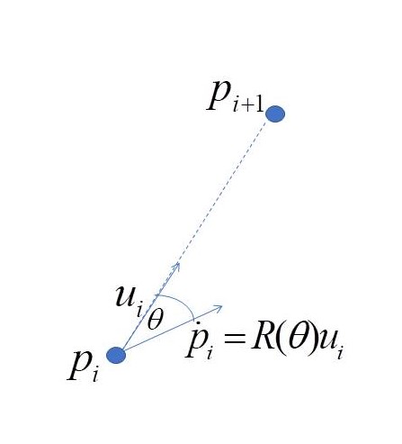
Figure 1: Illustration of deviated pursuit

The deviation angle $\theta$ is assumed to be constant and common to all agents.

1.1 Literature survey

Various researchers have treated the problem of formations obtained in autonomous cyclic pursuit, without external input. In the sequel we refer to those considering agents modeled as single-integrators with linear dynamics. The problem of linear agreement algorithms for agents with single integrator kinematics, over general topologies, was vastly investigated (see e.g. [3],[7], [6], [13]). Cyclic pursuit is a particular unidirectional topology where each agent receives information from a single neighbor, its target.

Lin et al. consider in [5] $n$ ordered and numbered points in the complex plane, each representing a freely mobile agent. They show that when the agents are in linear cyclic pursuit they converge to the centroid of the points and the centroid is stationary. Moreover, other formations are achievable by a simple modification, where each agent chases a ”fixed” displacement of its target.

Sinha and Goose, [15], consider a group of autonomous mobile agents, with identical behavior rules but with generally different control gains

$$\dot{p}_{i} = u_{i}$$

$$u_{i} = k_{i}(p_{i+1}-p_{i})$$

for $i=1,\dots,n$. They show that, by suitably selecting the gains $k_{i}$, the collective behavior of the agents can be controlled to obtain not only a point of convergence but also directed motion, where the trajectories of all the agents converge to a straight line as $t\rightarrow\infty$, (see conditions in Theorem 3, Theorem 4).

Pavone and Frazzoli, [8], generalize the (linear) cyclic pursuit strategy to deviated cyclic pursuit, in the context of geometric pattern formation. They show that $n$ agents operating in $\mathbb{R}^{2}$, in deviated cyclic pursuit, with a common offset angle $\theta$, will eventually converge to a single point, a circle or an ever expanding logarithmic spiral pattern, depending on the value of $\theta$, as follows:

• if $|\theta|<\pi/n$, to a single point, determined by the initial positions of the agents (the initial centroid)

• if $|\theta|=\pi/n$, to an evenly spaced circle formation, with radius determined by the initial positions of the agents

• if $\pi/n<|\theta|<2\pi/n$, to an evenly spaced, ever expanding, logarithmic spiral formation.

Ramirez et al. in [10], [9], extended these results in three directions:

1. the agents move in $\mathbb{R}^{3}$

2. control of the center of the formation by modifying the autonomous velocity control

   $$u_{i} = R(\theta)(p_{i+1}-p_{i})-k_{c}p_{i};\quad k_{c}\geq 0$$

   $$\dot{p}_{i} = u_{i}$$

   If $k_{c}>0$ then

   1. the center of the formation is no longer determined by the initial positions of the agents, instead it always converges, exponentially fast, to the origin.

   2. each agent is required to know not only the relative position to its target but also its own position, (in contradiction to our requirements here).

3. control the radius of the evenly-spaced circular formations.
   The key idea here is to relax the assumption of a common deviaton angle, $\theta$, and make the deviation angle of each agent, $\theta_{i}$, a function of the location of the agents and the desired inter-agent distance. In this case, the rule of motion (1) becomes

   $$\dot{p}_{i}=R(\theta_{i})(p_{i+1}-p_{i})$$

   where

   $$\theta_{i}=\frac{\pi}{n}+k_{th}(r-\|p_{i+1}-p_{i}\|);\quad r,k_{th}>0$$

   and $r$ is the desired inter-agent distance and $k_{th}$ is a gain.

Ren considered more general topologies and shows that collective motions including rendezvous, circular patterns, and logarithmic spiral patterns can be achieved by introducing Cartesian coordinate coupling to existing consensus algorithms. A particular case of coupling is the rotation matrix. In [11] the effect of coordinates coupling, introduced by a rotation matrix, on linear consensus algorithms for agents with single integrator kinematics was considered. In this case, the rule of movement is

$$\dot{p}_{i}=\sum_{k\in N_{i}}R(\theta)(p_{k}-p_{i})$$ (3)

where $R(\theta)$ is the rotation matrix and $N_{i}$ is the neighborhood of agent $i$, representing a general network topology, in contrast to [8], where the analysis of a similar problem was limited to unidirectional ring topology (cyclic pursuit). It is shown that both the network topology and the value of the rotation angle affect the resulting collective motions. When the nonsymmetric Laplacian matrix, representing the network topology, has certain properties and the rotation angle is below, equal, or above a critical value, the agents will eventually rendezvous, move on circular orbits, or follow logarithmic spiral curves. In particular, when the agents eventually move on circular orbits, the relative radius of the orbits is equal to the relative magnitude of the components of a right eigenvector associated with a critical eigenvalue of the nonsymmetric Laplacian matrix, in contrast to the common circular obits obtained in case of cyclic pursuit (see [8]).

1.2 An Overview of The New Results

The contribution of this work is in the analysis of the impact of an exogenous velocity control on the emergent behavior of $n$ agents performing (autonomous) deviated linear cyclic pursuit. The exogenous velocity control, we assume, is broadcast by a controller and detected by a random set of agents from the group, that thereby become temporary (ad-hoc) ”leaders” of the swarm.

In this case, the rule of movement (1) becomes

$$\dot{p}_{i}(t)=R(\theta)(p_{i+1}(t)-p_{i}(t))+b_{i}(t)U_{c}(t);\quad i=1,...,n$$ (4)

where

• $U_{c}(t)$ is the broadcast velocity vector signal at time $t$

• $b_{i}(t)$ is the indicator of detection of $U_{c}(t)$ by agent $i$, given by

  $$b_{i}=\begin{cases}1\quad&\text{if agent }$i$\text{ detects }U_{c}\\ 0\quad&\text{otherwise}\end{cases}$$ (5)

1.2.1 Group dynamics with broadcast control

Let $P=\left[p_{1},p_{2},...p_{n}\right]^{T}$ be the vector of stacked agent positions, where $p_{i},\quad i=1,\dots,n$ evolves according to eq. (4). The group dynamics of the system can be written as:

$$\dot{P}(t)=\hat{M}P(t)+\hat{B}(t)U_{c}(t)$$ (6)

where

• $\hat{M}=M\otimes R(\theta)$, such that $M$ is the circulant matrix (7):

  $$M_{n\times n}=circ[-1,1,0,0,\ldots,0]=\begin{bmatrix}-1&1&0&0&\ldots&0\\ 0&-1&1&0&\ldots&0\\ &&\vdots\\ 1&0&&\ldots&0&-1\\ \end{bmatrix}$$ (7)

  and $R(\theta)$ is defined by (2).

• $\hat{B}(t)=B(t)\otimes I$, where $B$ is the ”leaders” indicator, i.e. $B_{n\times 1}(i)=b_{i}$, where $b_{i}$ is defined by (5) and $I$ is the $2\times 2$ identity matrix

• $\otimes$ denotes the Kronecker product, see Appendix B

• $U_{c}$ is the external broadcast control, $U_{c}(t)\in\mathbb{R}^{2}$

Due to the structure of $M$, $\hat{M}$ is block circulant, as follows:

$$\hat{M}=\begin{bmatrix}-R(\theta)&R(\theta)&0_{2\times 2}&0_{2\times 2}&\ldots&0_{2\times 2}\\ \\ 0_{2\times 2}&-R(\theta)&R(\theta)&0_{2\times 2}&\ldots&0_{2\times 2}\\ \\ &&\vdots\\ \\ R(\theta)&0_{2\times 2}&\ldots&&0_{2\times 2}&-R(\theta)\end{bmatrix}$$ (8)

The matrix $M$ is time independent by its definition (see (7)). The assumption of cyclic pursuit with a constant deviation angle makes $R(\theta)$, and therefore $\hat{M}$ too, time independent. We assume the exogenous control, $U_{c}(t)$, and the set of agents detecting it, defined by the leaders indicator vector $B(t)$, to be piecewise constant. In the sequel we treat separately each interval where $U_{c}(t)$ and $B(t)$ ( the set of agents detecting the exogenous control) are constant and thus it is convenient to let $t$ denote the relative time since the beginning of the interval and $P(0)$ the state of the system at the moment of change, defined to be $t=0$.

Remark 1.1.

The behavior of the group of agents in multiple intervals, where $U_{c}$ and/or $B$ change at the start of each new interval and the end conditions of one interval are the start conditions of the next interval, is discussed and illustrated by simulation in section 3.2.2.

In each interval eq. (6) becomes

$$\dot{P}(t)=\hat{M}P(t)+\hat{B}U_{c}$$ (9)

i.e. the system evolves as a linear time independent system (LTI) with the well known solution (10), (see [4]).

$$P(t)=e^{\hat{M}t}P(0)+\int_{0}^{t}e^{\hat{M}(t-\tau)}\hat{B}U_{c}\mathrm{d}\tau$$ (10)

1.2.2 The resulting emergent behavior

Given an external broadcast control, $U_{c}$, the emergent behavior of the group is a function of the deviation angle $\theta$, the critical angle, $\displaystyle\theta_{c}=\frac{\pi}{n}$ and the (random) subset of agents detecting the broadcast control (leaders), represented by the leaders indicator vector $B$. We have the following results:

• if $\theta<\theta_{c}$ then

  • if $B=\mathbf{1}_{n}$, i.e. all agents detect the broadcast control signal, then the asymptotic behavior of the group is given by

    $$\boxed{p_{i}(t\rightarrow\infty)=p_{c}+U_{c}t;\quad i=1,\dots,n}$$

    where $p_{c}$ is the centroid of the initial positions. Thus, if all agents detect the broadcast control, the agents will eventually gather and move as a single point with velocity $U_{c}$ on a line anchored at $p_{c}$.

  • if $B\neq\mathbf{1}_{n}$ then

    $$\boxed{p_{i}(t\rightarrow\infty)=p_{c}+\frac{n_{l}}{n}U_{c}t+\sigma_{i}R(-\theta)U_{c};\quad i=1,\dots,n}$$

    In this case, all agents will eventually move with velocity $\frac{n_{l}}{n}U_{c}$ on parallel lines anchored at $p_{c}+\sigma_{i}R(-\theta)U_{c}$, where

    • $n_{l}$ is the number of agents detecting $U_{c}$.

    • $\sigma_{i}R(-\theta)U_{c}$ is the asymptotic deviation of the anchor of the movement line of agent $i$ from the centroid $p_{c}$ and $\sigma_{i}$ is a function of $B$, i.e. of the set of leaders (see section 2.2.2)

    Therefore, the agents will asymptotically align in a linear formation, rotated by $-\theta$ from the direction of $U_{c}$, and the formation will move with velocity $\displaystyle\frac{n_{l}}{n}U_{c}$.

• if $\theta=\theta_{c}$ then

  • if $B=\mathbf{1}_{n}$ then

    $$\boxed{p_{i}(t\rightarrow\infty)=p_{c}+U_{c}t+p^{r}_{i}(t);\quad i=1,\dots,n}$$

    where

    • $p^{r}_{i}(t)$ is a rotation component of the position at time $t$, s.t.

      $$\boxed{p^{r}_{i}(t)=[r\sin(\omega t+\alpha_{i}),r\cos(\omega t+\alpha_{i})]^{T}}$$

    • $\omega=2\sin(\frac{\pi}{n})$

    • $R$ is the radius of a circular orbit, common to all agents, determined by the number of agents and the initial positions

    • The agents are equally spaced on the orbit, at angular distance $\displaystyle\frac{2\pi}{n}$, i.e. $\displaystyle\alpha_{i+1}-\alpha_{i}=\frac{2\pi}{n}$

    Therefore, the agents are asymptotically moving, at equal distances, on a circular orbit, around a common center moving with velocity $U_{c}$.

  • if $B\neq\mathbf{1}_{n}$ then

    $$\boxed{p_{i}(t\rightarrow\infty)=p_{c}+\frac{n_{l}}{n}U_{c}t+p^{r}_{i}(t)+\tilde{\sigma_{i}}R(-\theta)U_{c};\quad i=1,\dots,n}$$

    where $p^{r}_{i}(t)$ is the position of agent $i$ on a common circular orbit, same as above, but in this case the center of the orbit, for agent $i$ is shifted by $\tilde{\sigma_{i}}R(-\theta)U_{c}$ from a common center, where $\tilde{\sigma_{i}}$ is a function of $B$ (see section 2.2.2). All centers move with velocity $\displaystyle\frac{n_{l}}{n}U_{c}$.

Remark 1.2.

We observe that the circular formation and its characteristics (radius and angular distances between agents) are independent of the broadcast control $U_{c}$ and the set of agents detecting it. These influence only the center of the orbit and its movement.

Remark 1.3.

The emergent behavior for the various deviation angles, summarized above, is determined by the eigenvalues of the matrix $\hat{M}$ (see Appendix D.1). We note that if $\theta>\theta_{c}$ then then $\hat{M}$ has at least two non-zero eigenvalues which lie in the open right-half complex plane causing the position of the agents to spiral out. This is an unstable system which is not discussed herein.

The emergent behaviors are rigorously derived in section 2 and illustrated by simulations in section 3.

1.3 Preliminaries - Properties of the matrix $\hat{M}$

The following properties of the matrix $\hat{M}$ are used in the sequel for the derivation of the emergent behavior of the system, $P(t\rightarrow\infty)$, evolving under (9).

• $\hat{M}$ is a normal matrix (see Lemma C.1), therefore it is unitarily diagonizable, i.e.

  $$\hat{M}=\Gamma\Lambda\Gamma^{*}$$

  where

  • $\Lambda$ is the diagonal matrix of eigenvalues of $\hat{M}$, denoted by
    $\mu_{k}^{\pm};\quad k=0,....,n-1$, (see Appendix D.1)

    $$\mu_{k}^{\pm}=2\sin(\frac{\pi k}{n})e^{-j(\frac{\pi}{2}+\frac{\pi k}{n}\pm\theta)}$$ (11)

  • $\Gamma$ is the unitary matrix of eigenvectors of $\hat{M}$, denoted by
    $\zeta_{k}^{\pm};\quad k=0,....,n-1$, see Appendix D.1, such that

    $$\zeta_{k}^{\pm}=v_{k}\otimes(1,\pm j)^{T}$$ (12)

    where

    $$v_{k}=\frac{1}{\sqrt{n}}\left(1,e^{-2\pi jk/n},e^{-4\pi jk/n},\ldots,e^{-2\pi jk(n-1)/n}\right)^{T};\quad k\in\left\{0,1,\ldots,n-1\right\}$$

• For $n$ agents in linear cyclic pursuit with common deviation angle $\theta$, there exists a critical value $\theta_{c}=\frac{\pi}{n}$, (see Corollary 2 in Appendix D.1.1), such that

  • if $|\theta|<\theta_{c}$, then $\hat{M}$ has two zero eigenvalues, $\mu_{0}^{\pm}$, and all other eigenvalues lie in the open left-half complex plane

  • if $|\theta|=\theta_{c}$, then $\hat{M}$ has two zero eigenvalues, $\mu_{0}^{\pm}$, and two non-zero eigenvalues which lie on the imaginary axis, while all remaining eigenvalues lie in the open left-half complex plane. The eigenvalues on the imaginary axis are $\mu_{n-1}^{+}$ and $\mu_{1}^{-}$

  • if $|\theta|>\theta_{c}$, then $\hat{M}$ has two zero eigenvalues and at least two non-zero eigenvalues which lie in the open right-half complex plane, therefore this is an unstable system which shall not be discussed herein. The agents in this case spread out and cease to remain in a finite extent constellation.

2 Derivation of The Emergent Behavior

We consider a piecewise constant time interval of a system evolving according to eq. (9), with a solution given by eq. (10). Since the emergent behavior is given by $P(t\rightarrow\infty)$ we assume that the dwell time of the interval is long enough to approach the asymptotic behavior. We recall (see eq. (10))

$$P(t)=e^{\hat{M}t}P(0)+\int_{0}^{t}e^{\hat{M}(t-\tau)}\hat{B}U_{c}\mathrm{d}\tau$$

which can be decomposed into

$$P(t)=P^{(h)}(t)+P^{(u)}(t)$$ (13)

where

• $\displaystyle P^{(h)}(t)=e^{\hat{M}t}P(0)$ is the homogeneous part of the solution, representing the zero input dynamics of the swarm

• $\displaystyle P^{(u)}(t)=\int_{0}^{t}e^{\hat{M}(t-\tau)}\hat{B}U_{c}\mathrm{d}\tau$ is the contribution of the guidance control, $U_{c}$, to the dynamics of the swarm

2.1 Zero input dynamics

$$P^{(h)}(t) = e^{\hat{M}t}P(0)$$ (14)

$$= \frac{1}{2}\sum_{i=0}^{n-1}[\zeta^{+}_{i}e^{\mu^{+}_{i}t}(\zeta^{+}_{i})^{*}+\zeta^{-}_{i}e^{\mu^{-}_{i}t}(\zeta^{-}_{i})^{*}]P(0)$$ (15)

where we used the decomposition property of $\hat{M}$ and $\mu_{i}^{\pm},\zeta_{i}^{\pm}$ are given by equations (11) and (12) respectively.

Separating in (15) the elements with zero eigenvalues from the remaining elements, we can rewrite (15) as

$$P^{(h)}(t)=P^{(h_{0})}+\Delta_{P}^{(h_{0})}(t)$$ (16)

where

• $P^{(h_{0})}$ is the component of the homogeneous position vector $P^{(h)}(t)$ due to the zero eigenvalues

  $$P^{(h_{0})}=\frac{1}{2}[\zeta^{+}_{0}(\zeta^{+}_{0})^{*}+\zeta^{-}_{0}(\zeta^{-}_{0})^{*}]P(0)$$ (17)

  $P^{(h_{0})}$ is time independent and common to all $\theta$, see section 2.1.1

• $\Delta_{P}^{(h_{0})}(t)$ is the component of $P^{(h)}(t)$, due to the remaining eigenvalues

  $$\Delta_{P}^{(h_{0})}(t)=\frac{1}{2}\sum_{i=1}^{n-1}[\zeta^{+}_{i}e^{\mu^{+}_{i}t}(\zeta^{+}_{i})^{*}+\zeta^{-}_{i}e^{\mu^{-}_{i}t}(\zeta^{-}_{i})^{*}]P(0)$$ (18)

  $\Delta_{P}^{(h_{0})}(t)$ is time dependent and its asymptotic value depends on $\theta$, see section 2.1.2

2.1.1 The derivation of $P^{(h_{0})}$

Lemma 2.1.

Let $P^{(h_{0})}:=(p_{1}^{(h_{0})},\dots,p_{n}^{(h_{0})})^{T}$ where $P^{(h_{0})}$ is defined by eq. (17). Denote by $p_{c}=(x_{c},y_{c})^{T}$ the centroid of the agents’ initial positions, $p_{i}(0)=(x_{i}(0),y_{i}(0))^{T}$.

Then

$$p_{i}^{(h_{0})}=p_{c};\quad\forall i\in[1,\dots,n]$$ (19)

Proof.

Recalling that the two eigenvectors of $\hat{M}$, corresponding to the two zero eigenvalues are $\zeta_{0}^{\pm}=v_{0}\otimes[1,\pm j]^{T}$ where $v_{0}=\mathbf{1}_{n}$ we have

$$\zeta_{0}^{\pm}=\frac{1}{\sqrt{n}}[1,\pm j,1,\pm j,\dots,1,\pm j]^{T}$$ (20)

Let $Y^{(0)}=\zeta^{+}_{0}(\zeta^{+}_{0})^{*}$. Then, eq. (17) can be rewritten as

$$P^{(h_{0})}=\frac{1}{2}(Y^{(0)}+\overline{Y^{(0)}})P(0)=\Re(Y^{(0)})P(0)$$

$$\Re(Y^{(0)})=\frac{1}{n}\begin{bmatrix}1&0&1&0\dots&1&0\\ 0&1&0&1\dots&0&1\\ \vdots&&&\dots&&\vdots\\ 1&0&1&0\dots&1&0\\ 0&1&0&1\dots&0&1\end{bmatrix}$$ (21)

Thus,

$$p_{i}^{(h_{0})}=(\frac{1}{n}\sum_{i=0}^{n-1}x_{i}(0),\frac{1}{n}\sum_{i=0}^{n-1}y_{i}(0))^{T}\equiv p_{c};\quad\forall i\in[1,\dots,n]$$ (22)

∎

2.1.2 Derivation of the asymptotic behavior of $\Delta_{P}^{(h_{0})}(t)$

$\Delta_{P}^{(h_{0})}(t)$ is the increment of the position, at time $t$, due to the eigenvalues other than the zero eigenvalues, see (16).

Lemma 2.2.

Let

$$\Delta_{P}^{(h_{0})}(t)=(\Delta_{p_{1}}^{(h_{0})}(t),\dots,\Delta_{p_{n}}^{(h_{0})}(t))^{T}$$ (23)

where $\Delta_{P}^{(h_{0})}(t)$ is defined as in eq. (18). Then $\Delta_{P}^{(h_{0})}(t\rightarrow\infty)$ is a function of $\theta$, as follows:

1. if $|\theta|<\theta_{c}$ then $\Delta_{p_{k}}^{(h_{0})}(t)\xrightarrow{t\to\infty}\mathbf{0}_{2};\forall k\in[1,\dots,n]$

2. if $|\theta|=\theta_{c}$ then the agents asymptotically move, equally spaced, on a common circular orbit.

   • The angular velocity is $\omega=2\sin(\frac{\pi}{n})$

   • The angular distance between consecutive agents is $\frac{2\pi}{n}$

   • The radius of the circular orbit is determined by the number of agents,$n$, and their initial positions $p_{l}(0);l=1,\dots,n$

Proof.

1. if $|\theta|<\theta_{c}$ , all non-zero eigenvalues of $\hat{M}$ have negative real part, see Corollary 2.(a), in Appendix D.1.1

   Thus, from eq. (18) we have $\Delta_{P}^{(h_{0})}(t)\xrightarrow{t\to\infty}\mathbf{0}_{2n}$. Therefore, according to (18),

   $$\Delta_{p_{k}}^{(h_{0})}(t)\xrightarrow{t\to\infty}\mathbf{0}_{2};\quad k=1,\dots,n$$

2. if $|\theta|=\theta_{c}$ , then in addition to the 2 zero eigenvalues, $\hat{M}$ has 2 eigenvalues on the imaginary axis $\mu_{n-1}^{+},\mu_{1}^{-}$ and all remaining eigenvalues of $\hat{M}$ have negative real part. Thus, $\Delta_{P}^{(h_{0})}(t)$ can be separated into a part containing the eigenvalues on the imaginary axis, denoted by $P^{(h_{1})}(t)$, and a part containing the remaining eigenvalues, which have negative real part, denoted by $P^{(h_{2})}(t)$.

   $$\Delta_{P}^{(h_{0})}(t)=P^{(h_{1})}(t)+P^{(h_{2})}(t)$$

   Since $P^{(h_{2})}(t)$ contains only eigenvalues with negative real part, we have

   $$P^{(h_{2})}(t)\xrightarrow{t\to\infty}\mathbf{0}_{2n}$$

   and

   $$\Delta_{P}^{(h_{0})}(t)\xrightarrow{t\to\infty}P^{(h_{1})}(t)=\frac{1}{2}[e^{\mu^{+}_{n-1}t}\zeta^{+}_{n-1}(\zeta^{+}_{n-1})^{*}+e^{\mu^{-}_{1}t}\zeta^{-}_{1}(\zeta^{-}_{1})^{*}]P(0)$$ (24)

   We show, in Appendix E that for $k=1,\dots,n$

   $$\Delta_{p_{k}}^{(h_{0})}(t)\xrightarrow{t\to\infty}:=p_{k}{(h_{1})}(t)=[r\sin(\omega t+\alpha_{k}),r\cos(\omega t+\alpha_{k})]^{T}$$

   where

   • $\omega=2\sin(\frac{\pi}{n})$

   • $r=\sqrt{c_{1}^{2}+c_{2}^{2}}$, where

     $$c_{1} = \frac{1}{n}\sum_{l=1}^{n}\left[\begin{matrix}\cos(\frac{2\pi}{n}l);&-\sin(\frac{2\pi}{n}l)\end{matrix}\right]p_{l}(0)$$

     $$c_{2} = \frac{1}{n}\sum_{l=1}^{n}\left[\begin{matrix}\sin(\frac{2\pi}{n}l);&\cos(\frac{2\pi}{n}l)\end{matrix}\right]p_{l}(0)$$

   • $\displaystyle\alpha_{k+1}=\alpha_{k}+\frac{2\pi}{n}$

   Therefore, the agents asymptotically move, equally spaced, on a circular orbit with a radius determined by the number of agents,$n$, and their initial positions $p_{l}(0);l=1,\dots,n$

∎

2.2 Input induced group dynamics

We recall, see eq. (13), that the position of the agents at time $t$ is given by

$$P(t)=P^{(h)}(t)+P^{(u)}(t)$$

where $P^{(h)}(t)$ is the homogeneous part of the solution, derived in section 2.1, and $P^{(u)}(t)$ is the contribution of the guidance control, $U_{c}$.

$$P^{(u)}(t)=\int_{0}^{t}e^{\hat{M}(t-\tau)}\hat{B}U_{c}\mathrm{d}\tau=\int_{0}^{t}\sum_{i=0}^{n-1}e^{\mu_{i}^{\pm}(t-\tau)}\hat{B}U_{c}\mathrm{d}\tau$$ (25)

where

• $\hat{B}=B\otimes I_{2\times 2}$

• $B$ is the indicator vector to the ad-hoc leaders (the agents detecting the exogenous control, $U_{c}$)

Recalling the location of the eigenvalues of $\hat{M}$, see Appendix D.1, we can write

$$P^{(u)}(t)=P^{(u_{1})}(t)+P^{(u_{2})}(t)+\Delta_{P}^{(u)}(t)$$ (26)

where

• $P^{(u_{1})}(t)$ is due to the elements with zero eigenvalue, existing for any $\theta$

• $P^{(u_{2})}(t)$ is due to the elements with $\mu_{1}^{-},\mu_{n-1}^{+}$ on the imaginary axis, existing if $\theta=\theta_{c}$

• $\Delta_{P}^{(u)}(t)$ is due to the remaining eigenvalues which have negative real part

2.2.1 Agents’ asymptotic velocity

$$V(t) = \frac{d}{dt}\left[P^{(u_{1})}(t)+P^{(u_{2})}(t)+\Delta_{P}^{(u)}(t)\right]$$

$$:= V^{(1)}(t)+V^{(2)}(t)+V^{(3)}(t)$$

$$V^{(3)}(t) = \frac{d}{dt}\Delta_{P}^{(u)}(t)$$

$$= \begin{cases}\sum_{i=1}^{n-1}e^{\mu_{i}^{\pm}t}\hat{B}U_{c}\quad&\text{if }|\theta|<\theta_{c}\\ \left(e^{\mu_{1}^{+}t}+e^{\mu_{n-1}^{-}t}+\sum_{i=2}^{n-1}e^{\mu_{i}^{\pm}t}\right)\hat{B}U_{c}\quad&\text{if }|\theta|=\theta_{c}\end{cases}$$

Since all $\mu_{i}$ in $V^{(3)}(t)$ have negative real part, we have

$$V^{(3)}(t)\xrightarrow{t\to\infty}\mathbf{0_{2n}}$$

Thus, the asymptotic velocity of agent $i$ is

$$V_{i}(t\rightarrow\infty)=V_{i}^{(1)}(t\rightarrow\infty)+V_{i}^{(2)}(t\rightarrow\infty)$$

Lemma 2.3.

Let $U_{c}$ be the broadcast velocity control, $B$ the ad-hoc leaders pointer vector, $n$ the number of agents and $n_{l}$ the number of agents detecting the broadcast control (ad-hoc leaders). Then,

1. if $|\theta|<\theta_{c}$ all agents move with asymptotic velocity $\displaystyle V_{i}(t\rightarrow\infty)=\frac{n_{l}}{n}U_{c}$.

2. if $|\theta|=\theta_{c}$ then the asymptotic velocities of the agents are

   $$V_{i}(t\rightarrow\infty)=\frac{n_{l}}{n}U_{c}+V_{i}^{c}(t)$$

   where $V_{i}^{c}(t)$ is the circular component of the velocity of agent $i$ at time $t$, such that

   $$V_{i}^{c}(t):=V_{i}^{(u_{2})}(t\to\infty)=\left[\begin{matrix}r^{V}\sin(\omega t+\alpha_{i}^{V})\\ r^{V}\cos(\omega t+\alpha_{i}^{V})\end{matrix}\right]$$

   where

   • $r^{V}$ is determined by $B$ and $U_{c}$ and is common to all agents

   • the phase shift between consecutive agents is $\displaystyle\frac{2\pi}{n}$

Proof.

1. Derivation of $V_{i}^{(u_{1})}(t)$

   $$P^{(u_{1})}(t)=\frac{1}{2}\left[\int_{0}^{t}(\zeta_{0}^{+}(\zeta_{0}^{+})^{*}+\zeta_{0}^{-}(\zeta_{0}^{-})^{*})\mathrm{d}\nu\right]\hat{B}U_{c}$$ (27)

   $\hat{B}=B\otimes I_{2\times 2}$.

   $$P^{(u_{1})}(t)=\frac{1}{2}t(\zeta_{0}^{+}(\zeta_{0}^{+})^{*}+\zeta_{0}^{-}(\zeta_{0}^{-})^{*})\hat{B}U_{c}$$ (28)

   Thus

   $$V^{(u_{1})}(t)=\frac{1}{2}(\zeta_{0}^{+}(\zeta_{0}^{+})^{*}+\zeta_{0}^{-}(\zeta_{0}^{-})^{*})\hat{B}U_{c}$$ (29)

   Using again $Y^{(0)}=\zeta^{+}_{0}(\zeta^{+}_{0})^{*}$ we obtain

   $$V^{(u_{1})}(t)=\Re(Y^{(0)})\hat{B}U_{c}$$ (30)

   where $\Re(Y^{(0)})$ is given by (21).

   $$\Rightarrow V_{i}^{(u_{1})}(t\to\infty)=\frac{n_{l}}{n}U_{c};\quad i=1,\dots,n$$

2. Derivation of $V_{i}^{c}(t)$

   $$P^{(u_{2})}(t)=\frac{1}{2}\left[\int_{0}^{t}(e^{\mu^{+}_{n-1}\nu}\zeta_{n-1}^{+}(\zeta_{n-1}^{+})^{*}+e^{\mu^{-}_{1}\nu}\zeta_{1}^{-}(\zeta_{1}^{-})^{*})\mathrm{d}\nu\right]\hat{B}U_{c}$$ (31)

   Thus

   $$V^{(u_{2})}(t) = \frac{d}{dt}P^{(u_{2})}(t)$$ (32)

   $$= \frac{1}{2}\left[e^{\mu^{+}_{n-1}t}\zeta_{n-1}^{+}(\zeta_{n-1}^{+})^{*}+e^{\mu^{-}_{1}t}\zeta_{1}^{-}(\zeta_{1}^{-})^{*}\right]\hat{B}U_{c}$$ (33)

   We note the similarity of eq. (33) to (24) with $\hat{B}U_{c}$ replacing $P(0)$. Therefore, we can write (by similarity)

   $$V_{i}^{c}(t):=V_{i}^{(u_{2})}(t\to\infty)=\left[\begin{matrix}r^{V}\sin(\omega t+\alpha_{i}^{V})\\ r^{V}\cos(\omega t+\alpha_{i}^{V})\end{matrix}\right]$$ (34)

   where

   • $\displaystyle\omega=2\sin(\frac{\pi}{n})$

   • $r^{V}=\sqrt{(c_{1}^{V})^{2}+(c_{2}^{V})^{2}}$, such that

     $$c_{1}^{V} = \frac{1}{n}\sum_{l=1}^{n}b_{l}\left[\begin{matrix}\cos(\frac{2\pi}{n}l);&-\sin(\frac{2\pi}{n}l)\end{matrix}\right]U_{c}$$

     $$c_{2}^{V} = \frac{1}{n}\sum_{l=1}^{n}b_{l}\left[\begin{matrix}\sin(\frac{2\pi}{n}l);&\cos(\frac{2\pi}{n}l)\end{matrix}\right]U_{c}$$

   • $\displaystyle\alpha_{i+1}^{V}=\alpha_{i}^{V}+\frac{2\pi}{n}$

∎

2.2.2 Contribution of remaining eigenvalues: $\Delta_{P}^{(u)}(t\to\infty)$

The eigenvalues whose contribution has not been considered so far are the eigenvalues with negative real part, causing element $\Delta_{P}^{(u)}$ in (26), due to the integration in $P^{(u)}(t)$, eq. (25). These eigenvalues are

• all eigenvalues other than $\mu_{0}^{\pm}$, if $\theta<\theta_{c}$

• all eigenvalues other than $\mu_{0}^{\pm},\mu_{1}^{-},\mu_{n-1}^{+}$ , if $\theta=\theta_{c}$

Let $p_{c}(t)$ denote the moving centroid at time $t\to\infty$, such that

$$p_{c}(t)=p_{c}(0)+\frac{n_{l}}{n}U_{c}$$

where $p_{c}(0)$ is the centroid of the initial positions. Then

$$p^{d}_{i}(t)=p_{c}(t)+\Delta_{p_{i}}^{(u)}$$ (35)

where $\Delta_{p_{i}}^{(u)};\quad i\in[1,\dots,n]$, such that $\Delta_{P}^{(u)}=(\Delta_{p_{1}}^{(u)},\dots,\Delta_{p_{n}}^{(u)})^{T}$, represents the asymptotic deviation of agent $i$ from $p_{c}(t)$.

• if $\theta<\theta_{c}$ then $p_{i}^{d}(t)$ is the position of agent $i$ at time $t\to\infty$

• if $\theta=\theta_{c}$ then $p_{i}^{d}(t)$ is the center of the circular orbit for agent $i$ at time $t\to\infty$

Lemma 2.4.

Let $p^{d}_{i}(t)$ be defined as in eq. (35). Then $p^{d}_{i}(t);i=1,\dots,n$ are aligned on a line rotated by angle $-\theta$ from the direction of $U_{c}$. The dispersion of the agents along this line is a function of the set of agents detecting the exogenous control,$U_{c}$, represented by the vector $B$.

Proof.

Consider the case $\theta<\theta_{c}$ . Then we have

$$\Delta_{p}^{(u)}(t) = \frac{1}{2}\left[\sum_{i=1}^{n-1}(\int_{0}^{t}(\zeta_{i}^{+}e^{\mu_{i}^{+}\nu}(\zeta_{i}^{+})^{*}+\zeta_{i}^{-}e^{\mu_{i}^{-}\nu}(\zeta_{i}^{-})^{*})\mathrm{d}\nu)\right]\hat{B}U_{c}$$

$$= \frac{1}{2}\sum_{i=1}^{n-1}[\frac{1}{\mu^{+}_{i}}(1-e^{\mu_{i}^{+}t})\zeta_{i}^{+}(\zeta_{i}^{+})^{*}+\frac{1}{\mu^{-}_{i}}(1-e^{\mu_{i}^{-}t})\zeta_{i}^{-}(\zeta_{i}^{-})^{*}]\hat{B}U_{c}$$

$$\triangleq \Delta_{P}^{(u_{1})}+\Delta_{P}^{(u_{2})}(t)$$

where

$$\Delta_{P}^{(u_{1})} = \frac{1}{2}\sum_{i=1}^{n-1}[\frac{1}{\mu^{+}_{i}}\zeta_{i}^{+}(\zeta_{i}^{+})^{*}+\frac{1}{\mu^{-}_{i}}\zeta_{i}^{-}(\zeta_{i}^{-})^{*}]\hat{B}U_{c}$$ (36)

$$\Delta_{P}^{(u_{2})}(t) = -\frac{1}{2}\sum_{i=1}^{n-1}[\frac{1}{\mu^{+}_{i}}e^{\mu_{i}^{+}t}\zeta_{i}^{+}(\zeta_{i}^{+})^{*}+\frac{1}{\mu^{-}_{i}}e^{\mu_{i}^{-}t}\zeta_{i}^{-}(\zeta_{i}^{-})^{*}]\hat{B}U_{c}$$ (37)

Since $\Re(\mu_{i})<0;i=1,\dots,n-1$ we have $\Delta_{P}^{(u_{2})}(t)\xrightarrow{t\to\infty}\mathbf{0}_{2n}$ and therefore

$$\Delta_{P}^{(u)}(t)\xrightarrow{t\to\infty}\Delta_{P}^{(u_{1})}$$

.

Recalling that (see Appendix D.1)

$$\mu_{i}^{\pm} = \lambda_{i}e^{\pm j\theta)}$$

$$\zeta_{i}^{\pm} = v_{i}\otimes(1,\pm j)^{T}$$

where $\lambda_{i},v_{i};\quad i=0,\dots,n-1$ are the eigenvalues and eigenvectors of $M$, respectively, and using the property of product of two Kronecker products, eq. (51), we have

$$\frac{1}{\mu^{+}_{i}}e^{\mu_{i}^{+}t}\zeta_{i}^{+}(\zeta_{i}^{+})^{*}=\frac{e^{-j\theta}}{\lambda_{i}}v_{i}v_{i}^{*}\otimes\left[\begin{matrix}1&-j\\ j&1\end{matrix}\right]$$

Similarly

$$\frac{1}{\mu^{-}_{i}}e^{\mu_{i}^{-}t}\zeta_{i}^{-}(\zeta_{i}^{-})^{*}=\frac{e^{j\theta}}{\lambda_{i}}v_{i}v_{i}^{*}\otimes\left[\begin{matrix}1&j\\ -j&1\end{matrix}\right]$$

Let

$$A=e^{-j\theta}\begin{bmatrix}1&-j\\ j&1\end{bmatrix}$$ (38)

Then,

$$\frac{1}{\mu^{+}_{i}}e^{\mu_{i}^{+}t}\zeta_{i}^{+}(\zeta_{i}^{+})^{*}+\frac{1}{\mu^{-}_{i}}e^{\mu_{i}^{-}t}\zeta_{i}^{-}(\zeta_{i}^{-})^{*}=\frac{2}{\lambda_{i}}v_{i}v_{i}^{*}\otimes\Re(A)$$

where

$$\Re(A)=\begin{bmatrix}\cos(\theta)&-\sin(\theta)\\ \sin(\theta)&\cos(\theta)\end{bmatrix}=R(-\theta)$$ (39)

where $R(\theta)$ is the rotation matrix defined in (2). Thus, we can rewrite eq. (36) as

$$\Delta_{P}^{(u_{1})} = \sum_{i=1}^{n-1}(\frac{1}{\lambda_{i}}v_{i}v_{i}^{*}\otimes R(-\theta))(B\otimes I)U_{c}$$ (40)

$$= ([\sum_{i=1}^{n-1}\frac{1}{\lambda_{i}}v_{i}v_{i}^{*}]B)\otimes R(-\theta)U_{c}$$ (41)

Given $\lambda_{i},v_{i};i=0,\dots,n-1$ as defined in (57), (54) respectively and $M=circ(-1,1,0,\dots,0)$ we have

$$v_{i}^{*}M^{T}=\overline{\lambda_{i}}v_{i}^{*}$$

Thus, we can rewrite (41) as

$$\Delta_{P}^{(u_{1})} = ([\sum_{i=1}^{n-1}\frac{1}{\lambda_{i}\overline{\lambda_{i}}}v_{i}v_{i}^{*}]M^{T}B)\otimes R(-\theta)U_{c}$$ (42)

$$:= (\gamma M^{T}B)\otimes R(-\theta)U_{c}$$ (43)

where

$$\gamma=[\sum_{i=1}^{n-1}\frac{1}{\lambda_{i}\overline{\lambda_{i}}}v_{i}v_{i}^{*}]$$ (44)

is an $n\times n$ matrix common to all agents. Let

$$\sigma=\gamma M^{T}B$$ (45)

Then we have

$$\Delta_{p_{i}}^{(u_{1})}=\sigma_{i}R(-\theta)U_{c}$$ (46)

where $\sigma_{i}$ is a scalar. Thus, the agents asymptotically align in a linear formation rotated by an angle $-\theta$ from the direction of $U_{c}$ . The dispersion of the agents along this line is a function of the set of agents detecting the exogenous control, represented by $B$.

Consider now the case $\theta=\theta_{c}$ .
In this case there are two additional eigenvalues of $\hat{M}$ with zero real part, $\mu_{1}^{-}$ and $\mu_{n-1}^{+}$, and following the same procedure as above, we have

$$\Delta_{P}^{(u_{1})} = \frac{1}{2}\left[\sum_{i=1}^{n-1}[\frac{1}{\mu^{+}_{i}}\zeta_{i}^{+}(\zeta_{i}^{+})^{*}-+\frac{1}{\mu^{-}_{i}}\zeta_{i}^{-}(\zeta_{i}^{-})^{*}]-\frac{1}{\mu^{-}_{1}}\zeta_{1}^{-}(\zeta_{1}^{-})^{*}-\frac{1}{\mu_{n-1}^{+}}\zeta_{n-1}^{+}(\zeta_{n-1}^{+})^{*}\right]\hat{B}U_{c}$$

$$= (\tilde{\gamma}M^{T}B)\otimes R(-\theta)U_{c}$$

where

$$\tilde{\gamma}=\gamma-\frac{1}{\lambda_{1}\overline{\lambda_{1}}}v_{1}v_{1}^{*}$$

and $\gamma$ is given by (44).

$$\Delta_{p_{i}}^{(u_{1})}=\tilde{\sigma}_{i}R(-\theta)U_{c}$$ (47)

where

$$\tilde{\sigma}=\tilde{\gamma}M^{T}B$$ (48)

∎

Remark 2.1.

If $B=\mathbf{1}_{n}$, i.e. the signal $U_{c}$ is detected by all the agents, then $\Delta_{p_{i}}^{(u)}=0;\forall i$ and therefore $p_{i}^{d}(t)=p_{c}(t);\forall i$. This is due to $M^{T}B=\mathbf{0}_{n}$ in the expression for $\sigma$ and $\tilde{\sigma}$, eqs. (45) and (48), respectively.

3 Demonstration by Simulation

In this section we illustrate by simulation the impact of the deviation angle $\theta$, of the broadcast control, $U_{c}(t)$, and of the set of leaders (agents detecting the broadcast control) on the emergent behavior of a group of agents in linear, deviated, cyclic pursuit. We recall that the set of agents detecting the broadcast control is represented by the vector $B$, such that $B(i)=1$ if agent $i$ detected the broadcast signal and $B(i)=0$ otherwise.

We present results for

1. Single time interval

   1. Autonomous deviated linear cyclic pursuit, without external control

   2. The broadcast control and the set of leaders are constant in the time interval, i.e. $U_{c}(t)=U_{c},B(t)=B$ for $t\in[0,T_{max}]$

2. Multiple time intervals, where the time line $[0,T_{max}]$ is divided in piecewise constant time intervals $[t_{k},t_{k+1}];\quad k=0,....m-1$, where $m$ is the number of intervals and

   • $U_{c}(t)=U_{c}(t_{k})$ if $t\in[t_{k},t_{k+1})$

   • $B(t)=B(t_{k})$ if $t\in[t_{k},t_{k+1})$

   • The start state of a new interval is the end state of the previous interval

In all shown simulation results we assumed $n=5$, where $n$ is the number of agents.

3.1 Autonomous deviated cyclic pursuit

In this section we illustrate the emergent behavior of the autonomous deviated cyclic pursuit, i.e. with $U_{c}=(0,0)^{T}$, as a function of the deviation angle $\theta$, corresponding to the analytically obtained results (see section 2.1). We recall that $\displaystyle\theta_{c}=\frac{2\pi}{n}$. Therefore, for $n=5$ we have $\theta_{c}=36deg$.

We show, starting from two initial topologies, shown in Figures 2, (see Example1) and 5,(see Example2), that

• if $\theta<\theta_{c}$ then the agents gather to $p_{c}$, the centroid of the agents’ initial positions, see Figures 3 and 6. In these figures

  • $p_{c}$ is the displayed initial centroid

  • $p_{i}(T_{max}):=(x_{i}(T_{max},y_{i}(T_{max}))^{T}$

  • $p_{i}(T_{max})==p_{c}\quad\forall i$, as expected.

• if $\theta=\theta_{c}$ then the agents will rotate around $p_{c}$ on a common orbit with a radius (displayed as $r$) depending on the initial positions of the agents, see Figures 4 and 7.

  In these figures we show the trajectories of the agents,
  $p_{i}(t);i=1,\dots,n;t\in[0,T_{max}]$ and the circular component of the trajectories (shown in black). We note that the center of the circular orbit is $p_{c}$, as expected.

3.1.1 Example1

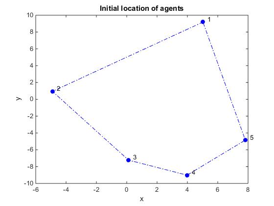
Figure 2: Example1 - Initial positions of the agents

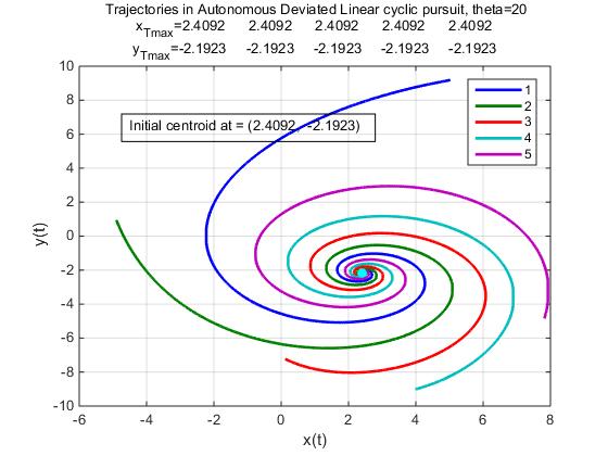
Figure 3: $\theta<\theta_{c}$ - Agents gathering to the centroid of the initial positions

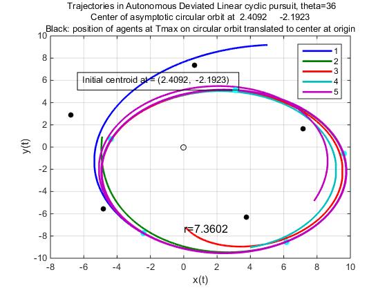
Figure 4: $\theta=\theta_{c}$ - Agents rotating around the centroid of the initial positions

3.1.2 Example2

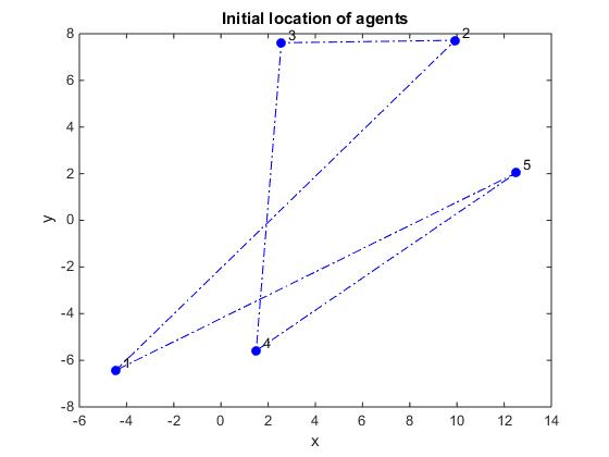
Figure 5: Example2 - Initial positions of the agents

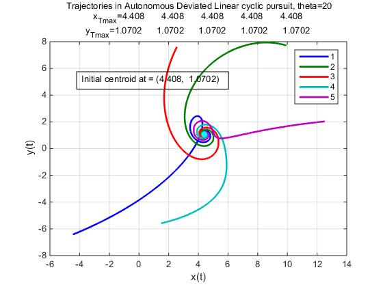
Figure 6: $\theta<\theta_{c}$ - Agents gathering to the centroid of the initial positions

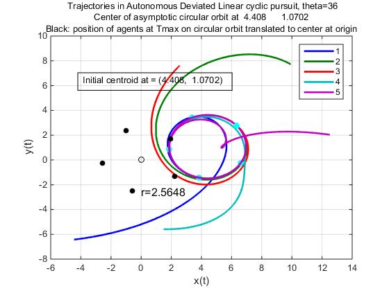
Figure 7: $\theta=\theta_{c}$ - Agents rotating around the centroid of the initial positions

3.2 The impact of the broadcast control and of the random set of leaders

The remaining simulations presented in this section were run with the initial locations shown in Figure 5.

In all the figures included in this section

• a solid line represents an ad-hoc leader (an agent that detects the broadcast control)

• a dotted line represents a follower (an agent that does not detect the broadcast control)

3.2.1 Single time interval

We recall that the emergent behavior, analytically derived in section 2, is an asymptotic behavior. Thus, in order to compare the numerical results, obtained by simulation to the analytically derived results we need the simulation time, $T_{max}$ to be long enough to approximate $t\rightarrow\infty$. We found that $T_{max}=60$ is such a time. Therefore all presented simulations were run with $T_{max}=60$ (Points=60000, dT=0.001). However, for visualization purposes all trajectories and velocities are shown for the first part of the data, up to $t=10$.

For the simulations presented in this section we used $U_{c}=(2,3)^{T}$ and we considered the following cases

1. $\theta=20deg(<\theta_{c})$

   1. $U_{c}$ is detected by all the agents, i.e. $B=\mathbf{1}_{n}$

   2. $U_{c}$ is detected only by agents 2 and 5, i.e $B=(0,1,0,0,1)^{T}$

2. $\theta=36deg(=\theta_{c})$

   1. $U_{c}$ is detected by all the agents, i.e. $B=\mathbf{1}_{n}$

   2. $U_{c}$ is detected only by agents 2 and 5, i.e $B=(0,1,0,0,1)^{T}$

Case 1.1: $\theta=20deg,\quad B=\mathbf{1}_{n}$

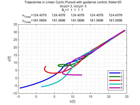
Figure 8: Case 1.1 - Emergent trajectories

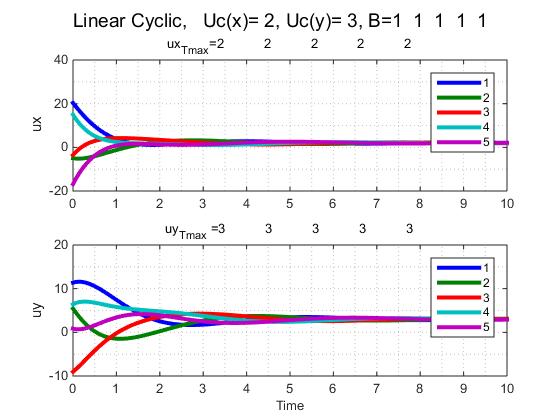
Figure 9: Case 1.1 - Emergent velocities

In this case all the agents converge to a point (see $x_{T_{max}},y_{T_{max}}$ in Fig. 8) that moves with asymptotic velocity $U_{c}$,(see $ux_{T_{max}},uy_{T_{max}}$ displayed in Fig. 9), as expected.

Case 1.2: $\theta=20deg,\quad B=(0,1,0,0,1)^{T}$

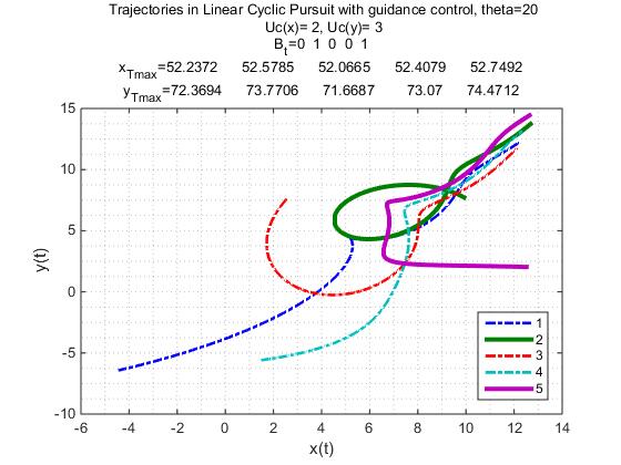
Figure 10: Case1.2 - Emergent trajectories

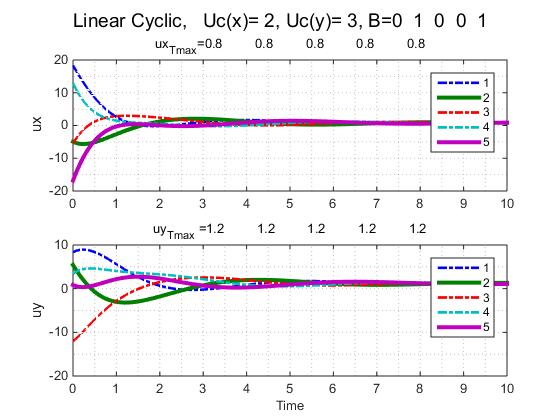
Figure 11: Case1.2 - Emergent velocities

In this case

• the number of ad-hoc leaders, $n_{l}$ is two.

• the velocity of each agent asymptotically converges to $\displaystyle\frac{n_{l}}{n}U_{c}$,
  see $(ux_{T_{max}},uy_{T_{max}})$ in Fig.11

• the emergent trajectories of the agents are parallel lines in the direction of $U_{c}$, anchored at $p_{c}+\Delta_{p_{i}}^{(u_{1})}$, (see Fig. 10) where $Delta_{p_{i}}^{(u_{1})}$ is the asymptotic, time independent, deviation given by eq. (46)

We complete the demonstration of the emergent behavior of the agents in case $\theta<\theta_{c},B\neq\mathbf{1}_{n}$ by showing the deviations of the agents from a moving center for $\theta=20\text{deg vs }0deg$, see Fig. 12. We observe that in both cases the agents are aligned in a linear formation. While for $\theta=0$ the formation is aligned with $U_{c}$ for $\theta=20$the formation is aligned with $R(-\theta)U_{c}$, where $R$ denotes the rotation matrix, complying with eq.(46).

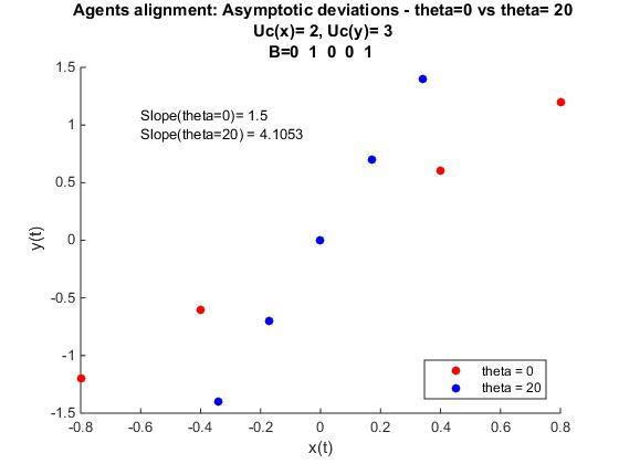
Figure 12: Agents’ asymptotic linear formation, $\theta=20\text{deg vs 0deg}$

In this case

$$R(-20)=\left[\begin{matrix}0.9397&-0.3420\\ 0.3420&0.9397\end{matrix}\right]$$

Thus, $R(-\theta)U_{c}$ has a slope= 4.1053, as indicated.

Case 2.1: $\theta=\theta_{c}=36deg,\quad B=\mathbf{1}_{n}$

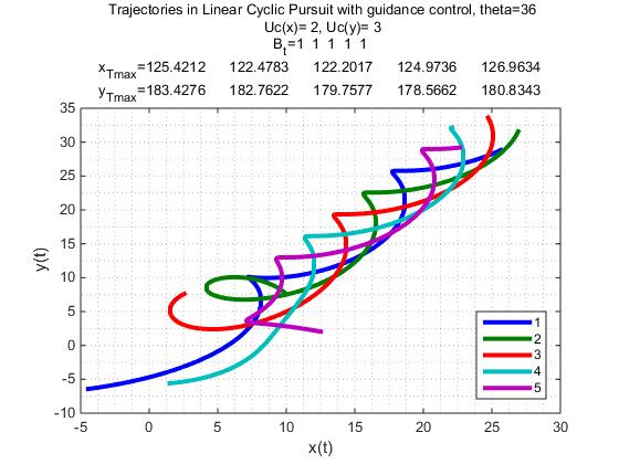
Figure 13: Case 2.1 - Emergent trajectories

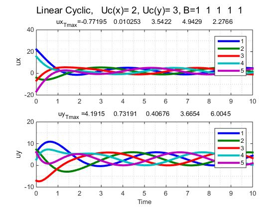
Figure 14: Case 2.1 - Emergent velocities

Case 2.2: $\theta=\theta_{c}=36deg,\quad B=(0,1,0,0,1)^{T}$

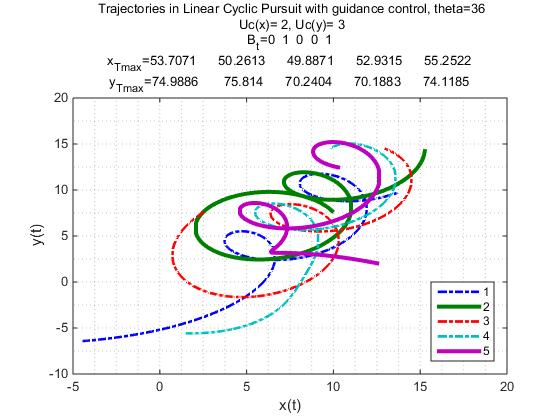
Figure 15: Case 2.2 - Emergent trajectories

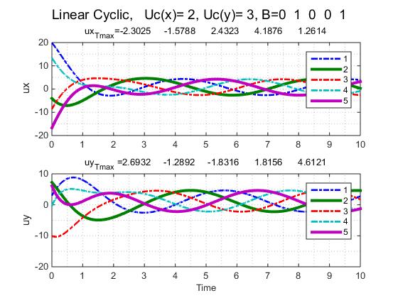
Figure 16: Case 2.2 - Emergent velocities

3.2.2 Multiple piecewise constant intervals

A new interval starts upon a change of broadcast velocity control, $U_{c}$, or a change in the set of agents detecting it, represented by the vector $B(t)$. The initial state of each interval is the end state of the previous interval.

In this section we show the emergent behavior of the same group of five agents, starting at the same initial positions, Fig. 5, over multiple intervals, with piecewise constant $U_{c}(t)$ and $B(t)$.

We show two cases of piecewise constant systems, $U_{c}(t)=(u_{x}(t),u_{y}(t))^{T}$ and $B(t)$, and for each system we show the emergent behavior, trajectories and velocities, for $\theta<\theta_{c}$ and $\theta=\theta_{c}$.

1. $U(t)$ as shown in Fig. 17, $B(t)$ as follows

   • for $t\in[0,45)$ the set of agents detecting the broadcast control is $\{2,5\}$, i.e. $B(t)=(0,1,0,0,1)^{T}$

   • for $t\in[45,60]$ the set of agents detecting the broadcast control is ”all”, i.e. $B(t)=\mathbf{1}_{5}$

2. $U(t)$ as shown in Fig. 18, $B(t)$ as follows

   • for $t\in[0,45)$ the set of agents detecting the broadcast control is $\{2,5\}$, i.e. $B(t)=(0,1,0,0,1)^{T}$

   • for $t\in[45,52.5)$ the set of agents detecting the broadcast control is ”all”, i.e. $B(t)=\mathbf{1}_{5}$

   • for $t\in[52.5,60]$ the set of agents detecting the broadcast control is again $\{2,5\}$, i.e. $B(t)=(0,1,0,0,1)^{T}$

We observe that the emergent behavior over multiple time intervals is a concatenation of the single intervals, as expected.

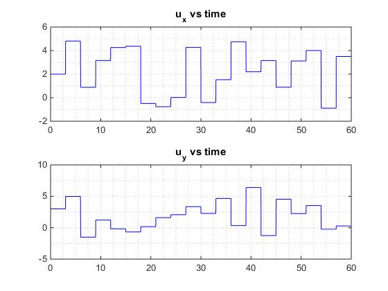
Figure 17: Piecewise constant broadcast control, $U_{c}(t)$ - CaseM.1

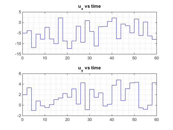
Figure 18: Piecewise constant broadcast control, $U_{c}(t)$ - CaseM.2

3.2.3 CaseM.1.1 - CaseM.1 with $\theta<\theta_{c}$

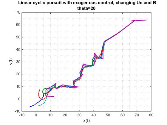
Figure 19: CaseM.1.1 - Emergent trajectories

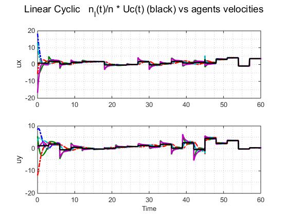
Figure 20: CaseM.1.1 - Emergent velocities

3.2.4 CaseM.1.2 - CaseM.1 with $\theta=\theta_{c}$

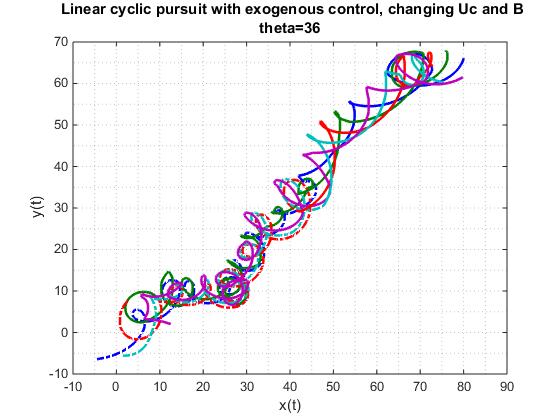
Figure 21: CaseM.1.2 - Emergent trajectories

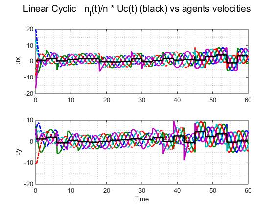
Figure 22: CaseM.1.2 - Emergent velocities

3.2.5 CaseM.2.1 - CaseM.2 with $\theta<\theta_{c}$

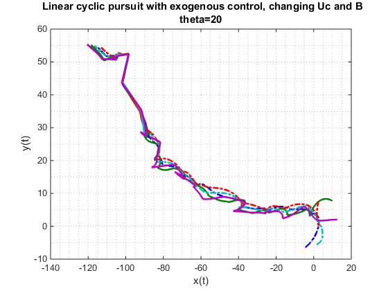
Figure 23: CaseM.2.1 - Emergent trajectories

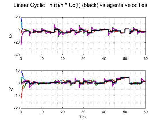
Figure 24: CaseM.2.1 - Emergent velocities

3.2.6 CaseM.2.2 - CaseM.2 with $\theta=\theta_{c}$

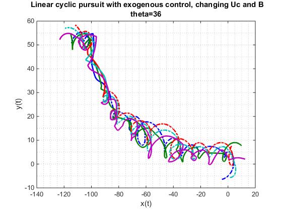
Figure 25: CaseM.2.2 - Emergent trajectories

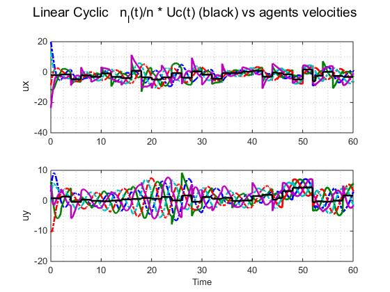
Figure 26: Example 2.2 - Emergent velocities

We note that what seems like an irregular circular movement in case $\theta=\theta_{c}$ and $B\neq\mathbf{1}_{n}$, see Fig. 21, 25, is actually due to changes in the deviation of the centers upon change in $U_{c}(t)$. (We recall that the deviation of the centers is given by eq. 46: $\Delta_{p_{i}}^{(u_{1})}=\sigma_{i}R(-\theta)U_{c}$). To demonstrate this claim we show the emergent behavior with the same $U_{c}(t)$ (see Fig. 18) in case $B=\mathbf{1}_{n}$, when the centers overlap, i.e. there are no deviations.

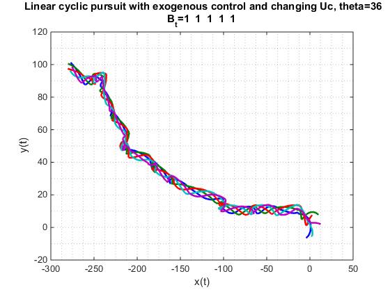
Figure 27: Emergent trajectories when $\theta=\theta_{c}$ and $B=\mathbf{1}_{n}$

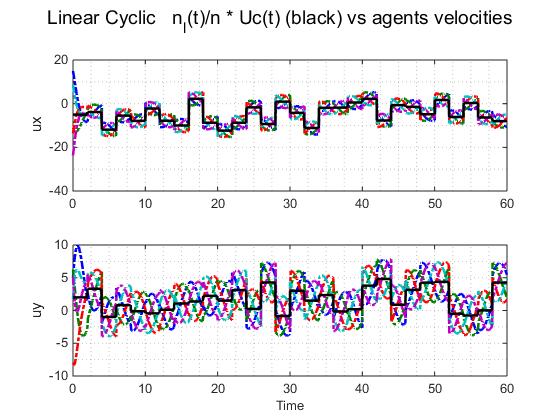
Figure 28: Emergent velocities when $\theta=\theta_{c}$ and $B=\mathbf{1}_{n}$

4 Summary and discussion

In this work we apply well known LTI systems evolution theory to a novel paradigm where agents in deviated linear cyclic pursuit are exposed to a piecewise constant broadcast control, detected by a random subset of agents. The emergent behavior of the agents is rigorously derived for a single time interval and illustrated by simulations for multiple time intervals, a concatenation of single time intervals. The emergent behavior of the swarm is shown to be a function of the deviation angle, $\theta$, the critical deviation angle $\displaystyle\theta_{c}=\frac{\pi}{n}$ and of the (random) subset of agents detecting the broadcast control (ad-hoc leaders). We show that the emergent pattern of movement depends only on the deviation angle $\theta$, such that

• if $\theta<\theta_{c}$ the movement is linear and the asymptotic velocity of the agents is $\displaystyle\frac{n_{l}}{n}U_{c}$, where $U_{c}$ is the broadcast control and $\displaystyle\frac{n_{l}}{n}$ is the ratio of agents detecting it.

  • If $\displaystyle\frac{n_{l}}{n}=1$ then the agents gather and move as a single point.

  • If $\displaystyle\frac{n_{l}}{n}<1$ then the agents will asymptotically move as a time independent linear formation rotated by $R(-\theta)$ from the direction of $U_{c}$.

• if $\theta=\theta_{c}$ the movement is circular around a center moving with velocity $\displaystyle\frac{n_{l}}{n}U_{c}$. The radius of the circular orbit is a function of the number of agents and the initial positions and is common to all agents.

  • If $\displaystyle\frac{n_{l}}{n}=1$ then the centers coincide. In this case the agents move, equally spaced, on a common orbit.

  • If $\displaystyle\frac{n_{l}}{n}<1$ then the centers move on parallel lines, such that at each point in time, $t$, they are placed on a line rotated by $R(-\theta)$ from the direction of $U_{c}$. The dispersion of the centers on this line is time-independent.

We plan in the future to investigate the emergent behavior of non-linear agents, sensing bearing-only (bugs), in deviated cyclic pursuit, under the influence of broadcast control detected by a random subset of agents.

Appendix A General results on matrices

Following [2], let $\mathbf{M}_{n}$ denote the class of all $n\times n$ matrices. Two matrices $A,B\in M_{n}$ are similar, denoted by $A\sim B$, if there exists an invertible (non-singular) matrix $S\in M_{n}$ s.t. $A=SBS^{-1}$. Similar matrices are just different basis representation of a single linear transformation.Similar matrices have the same characteristic polynomial, c.f. Theorem 1.3.3 in [2] and therefore the same eigenvalues

A.1 Algebraic and geometric multiplicity of eigenvalues

Let $\lambda$ be an eigenvalue of an arbitrary matrix $A\in M_{n}$ with an associated eigenvector $v\in\mathbb{C}^{n}$.
Definitions:

• The spectrum of $A\in M_{n}$ is the set of all the eigenvalues of $A$, denoted by $\sigma(A)$.

• The spectral radius of $A$ is $\rho(A)=max{|\lambda|:\lambda\in\sigma(A)}$.

• For a given $\lambda\in\sigma(A)$ , the set of all vectors $v\in\mathbb{C}^{n}$ satisfying $Av=\lambda v$ is called the eigenspace of $A$ associated with the eigenvalue $\lambda$ . Every nonzero element of this eigenspace is an eigenvector of $A$ associated with $\lambda$

• The algebraic multiplicity of $\lambda$ is its multiplicity as a root of the characteristic polynomial $det(\lambda I-A)$

• The geometric multiplicity of $\lambda$ is the dimension of the eigenspace associated with $\lambda$, i.e. the number of linearly independent eigenvectors associated with that eigenvalue.

• We say that $\lambda$ is simple if its algebraic multiplicity is 1; it is semisimple if its algebraic and geometric multiplicities are equal.

• The algebraic multiplicity of an eigenvalue is larger than or equal to its geometric multiplicity.

• We say that $A$ is defective if the geometric multiplicity of some eigenvalue is less than its algebraic multiplicity

A.2 Diagonizable matrices

Definition: If $A\in M_{n}$ is similar to a diagonal matrix, then $A$ is said to be diagonizable

Theorem 1.

See Theorem 1.3.7 in [2].

The matrix $A\in M_{n}$ is diagonizable iff there are $n$ linearly independent vectors, $v^{(1)},v^{(2)},....,v^{(n)}$, each of which is an eigenvector of $A$. If $v^{(1)},v^{(2)},....,v^{(n)}$ are linearly independent eigenvectors of $A$ and $S=[v^{(1)},v^{(2)},....,v^{(n)}]$ then $S^{-1}AS$ is a diagonal matrix $\Lambda$ and the diagonal entries of $\Lambda$ are the eigenvalues of $A$

Lemma 1.

Let $\lambda_{1},...,\lambda_{k};\quad k\geq 2$ be distinct eigenvalues of $A\in M_{n}$ and suppose $v^{(i)}$ is an eigenvector associated with $\lambda_{i};\quad i=1,....,n$. Then the vectors $[v^{(1)},v^{(2)},....,v^{(k)}]$ are linearly independent.

Proof of Lemma 1.3.8 in [2]

Theorem 2.

If $A\in M_{n}$ has $n$ distinct eigenvalues, then $A$ is diagonizable

Proof.

Since all eigenvalues are distinct Lemma 1 ensures that the associated eigenvectors are linearly independent and thus, according to Theorem 1, $A$ is diagonizable ∎

Notes:

1. Having distinct eigenvalues is sufficient for diagonizability, but not necessary.

2. A matrix is diagonizable iff it is non-defective, i.e. it has no eigenvalue with geometric multiplicity strictly less than its algebraic multiplicity

A.3 Left eigenvectors

Definition: A non-zero vector $y\in\mathcal{C}^{n}$ is a left eigenvector of $A\in M_{n}$ associated with eigenvalue $\lambda$ of $A$ if $y^{*}A=\lambda y^{*}$. From [2], Theorem 1.4.12, we have the following relationship between left and right eigenvectors and the multiplicities of the corresponding eigenvalue:

Theorem 3.

Let $\lambda\in\mathcal{C}$ be an eigenvalue of $A\in M_{n}$ associated with right eigenvector $x$ and left eigenvector $y^{*}$. Then the following hold:

1. If $\lambda$ has algebraic multiplicity 1, then $y^{*}x\neq 0$

2. If $\lambda$ has geometric multiplicity 1, then it has algebraic multiplicity 1 iff $y^{*}x\neq 0$

A.4 Square matrices decomposition

• If $A\in\mathbf{M}_{n}$ with distinct eigenvectors (not necessarily distinct eigenvalues) then $A=V\Lambda V^{-1}$, where $\Lambda$ is a diagonal matrix formed from the eigenvalues of $A$, and the columns of $V$ are the corresponding eigenvectors of $A$.
  A matrix $A\in\mathbf{M}_{n}$ always has $n$ eigenvalues, which can be ordered (in more than one way) to form a diagonal matrix $\Lambda\in\mathbf{M}_{n}$ and a corresponding matrix of nonzero columns $V$ that satisfies the eigenvalue equation $AV=V\Lambda$. If the $n$ eigenvectors are distinct then $V$ is invertible, implying the decomposition $A=V\Lambda V^{-1}$.
  Comment: The condition of having $n$ distinct eigenvalues is sufficient but not necessary. The necessary and sufficient condition is for each eigenvalue to have geometric multiplicity equal to its algebraic multiplicity.

• If $A$ is real-symmetric its $n$ (possibly not distinct) eigenvalues are all real with geometric multiplicity which equals the algebraic multiplicity. $V$ is always invertible and can be made to have normalized columns. Then the equation $VV^{T}=I$ holds, because each eigenvector is orthonormal to the other. Therefore the decomposition (which always exists if $A$ is real-symmetric) reads as: $A=V\Lambda V^{T}$. This is known as the the spectral theorem, or symmetric eigenvalue decomposition theorem.

• If $A\in\mathbf{M}_{n}$ is normal, i.e. $AA^{T}=A^{T}A$, then

  1. There exists an orthonormal set of $n$ eigenvectors of $A$

  2. $A$ is unitarily diagonizable, i.e. $A=U\Lambda U^{*}$, where $U$ is a unitary matrix of eigenvectors and $\Lambda$ is a diagonal matrix of eigenvalues of $A$.

A.5 About non-symmetric real matrices

• the eigenvalues of non-symmetric real $n\times n$ matrix are real or come in complex conjugate pairs

• the eigenvectors are not orthonormal in general and may not even span an n-dimensional space

  • Incomplete eigenvectors can occur only when there are degenerate eigenvalues, i.e. eigenvalues with algebraic multiplicity greater than 1, but do not always occur in such cases

  • Incomplete eigenvectors never occur for the class of normal matrices

• Diagonalization theorem: an $n\times n$ matrix $A$ is diagonizable iff $A$ has $n$ linearly independent eigenvectors

A.6 Normal matrices

Definition 1.

A matrix $A\in M_{n}$ is called normal if $A^{*}A=AA^{*}$

Definition 2.

A matrix $A\in M_{n}$ is called Hermitian if $A^{*}=A$

Theorem 4.

If $A\in M_{n}$ has eigenvalues $\lambda_{1},\lambda_{2},.....,\lambda_{n}$ the following statements are equivalent:

1. $A$ is normal

2. $A$ is unitarily diagonizable

3. $\sum_{i=1}^{n}\sum_{j=1}^{n}|a_{ij}|^{2}=\sum_{j=1}^{n}|\lambda_{j}|^{2}$

4. There is an orthonormal set of $n$ eigenvectors of $A$

Remark A.1.

All normal matrices are diagonizable but not all diagonizable matrices are normal.

A.7 Unitary matrices and unitary similarity

Unitary matrices, $U\in M_{n}$, are non-singular matrices such that $U^{-1}=U^{*}$, i.e $U^{*}U=UU^{*}=I$. A real matrix $U\in M_{n}(\mathbb{R})$ is real orthogonal if $U^{T}U=I$. The following are equivalent:

1. $U$ is unitary

2. $U$ is non-singular and $U^{-1}=U^{*}$

3. $UU^{*}=I$

4. $U^{*}$ is unitary

5. The columns of $U$ are orthonormal

6. The rows of $U$ are orthonormal

7. For all $x\in\mathcal{C}^{n},\quad\|x\|_{2}=\|Ux\|_{2}$

Definition A.1.

:

• $A$ is unitarily similar to $B$ if there is a unitary matrix $U$ s.t. $A=UBU^{*}$

• $A$ is unitarily diagonizable if it is unitarily similar to a diagonal matrix

Appendix B Kronecker product properties

This section follows mostly reference [12].

Definition B.1.

The Kronecker product of the matrix $A\in\mathbf{M}^{p,q}$ with the matrix $B\in\mathbf{M}^{r,s}$ is defined as

$$A\otimes B=\begin{bmatrix}A_{11}B&A_{12}B&\ldots&A_{1q}B\\ A_{21}B&A_{22}B&\ldots&A_{2q}B\\ &&\vdots\\ A_{p1}S&A_{p2}B&\ldots&A_{pq}B\\ \end{bmatrix}$$ (49)

B.1 Basic Properties

The properties of the Kronecker product in this subsection are only those with bearing on this work. A complete list of properties can be found in [12].

• Taking the transpose before carrying out the Kronecker product yields the same result as doing so afterwards, i.e.

  $$(A\otimes B)^{T}=A^{T}\otimes B^{T}$$ (50)

• The product of two Kronecker products yields another Kronecker product:

  $$(A\otimes B)(C\otimes D)=AC\otimes BD;\quad\forall A\in\mathbf{M}^{p,q},B\in\mathbf{M}^{r,s},C\in\mathbf{M}^{q,k},D\in\mathbf{M}^{s,l}$$ (51)

• Taking the complex conjugate before carrying out the Kronecker product yields the same result as doing so afterwards, i.e.

  $$(A\otimes B)^{*}=A^{*}\otimes B^{*};\quad\forall A\in\mathbf{M}^{p,q}(\mathbb{C}),B\in\mathbf{M}^{r,s}(\mathbb{C})$$ (52)

• Denote by $\sigma(A)$ the spectrum of a square matrix $A$, i.e. the set of all eigenvalues of $A$. Then, Theorem B.1 holds.

  Theorem B.1.

  (Theorem 2.3 in [12]) Let $A\in\mathbf{M}^{m}$ and $B\in\mathbf{M}^{n}$. Furthermore, let $\lambda\in\sigma(A)$ with corresponding eigenvector $x$ and let $\mu\in\sigma(B)$ with corresponding eigenvector $y$. Then, $\lambda\mu$ is an eigenvalue of $A\otimes B$ with corresponding eigenvector $x\otimes y$

Appendix C Properties of circulant matrices

A circulant matrix is an $n\times n$ matrix having the form

$$C=\begin{bmatrix}c_{0}&c_{1}&c_{2}&\ldots&c_{n-1}\\ c_{n-1}&c_{0}&c_{1}&\ldots&c_{n-2}\\ &&\vdots\\ c_{1}&c_{2}&&\ldots&c_{0}\\ \end{bmatrix}$$ (53)

which can also be characterized as an $n\times n$ matrix $C$ with entry $(k,j)$ given by

$$C_{k,l}=c_{(l-k)mod(n)}$$

Every $n\times n$ circulant matrix $C$ has eigenvectors (cf. [1], [10])

$$v_{k}=\frac{1}{\sqrt{n}}\left(1,e^{-2\pi jk/n},e^{-4\pi jk/n},\ldots,e^{-2\pi jk(n-1)/n}\right)^{T};\quad k\in\left\{0,1,\ldots,n-1\right\}$$ (54)

where $j=\sqrt{-1}$, with corresponding eigenvalues

$$\lambda_{k}=\sum_{l=0}^{n-1}c_{l}e^{-2\pi jlk/n}$$ (55)

From the definition of eigenvalues and eigenvectors we have

$$Cv_{k}=\lambda_{k}v_{k};\quad k=0,1,\ldots,n-1$$

which can be written as a single matrix equation

$$CU=U\Lambda$$

where $\Lambda=diag(\lambda_{k});\quad k=0,\ldots,n-1$ and

$$U = \left[v_{0},v_{1},\ldots,v_{n-1}\right]$$

$$= \frac{1}{\sqrt{n}}\left[e^{-2\pi jmk/n};\quad m,k=0,\ldots,n-1\right]$$

$U$ is a unitary matrix, i.e. $UU^{*}=U^{*}U=I$ (cf. [1], proof by direct computation) and

$$C=U\Lambda U^{*}$$ (56)

Note that $F_{n}=\sqrt{n}U^{*}$ is the known Fourier matrix.

C.1 Cyclic linear pursuit

The matrix $M$, representing cyclic pursuit, is a special case of circulant matrix (see eq. (7) $M=circ(-1,1,0,0,\dots,0)$.

Thus, using (55), the eigenvalues of $M$ are

$$\lambda_{k}=-1+e^{-2\pi jk/n};\quad k=0,...,n-1$$ (57)

and the eigenvectors are given by eq. (54).

Lemma C.1.

$M=circ(-1,1,0,0,\dots,0)$ is a normal matrix, i.e. satisfies $MM^{T}=M^{T}M$

Proof.

By direct computation $MM^{T}=M^{T}M=circ([2,-1,0,....,0,-1])$ ∎

Appendix D Properties of the block circulant matrix $\hat{M}$

Consider now the block circulant matrix $\hat{M}$, defined as in eq. (8), representing linear cyclic pursuit with a common deviation angle $\theta$.

$$\hat{M}=M\otimes R(\theta)$$

Thus, $\hat{M}=circ\left[-R(\theta),R(\theta),0_{2\times 2},...,0_{2\times 2}\right]$, where $R(\theta)$ is the rotation matrix, defined by eq. (2)

Lemma D.1.

The matrix $\hat{M}=M\otimes R(\theta)$, where $M=circ(-1,1,0,0,\dots,0)$ and $R$ is a rotation matrix, is a normal matrix

Proof.

Using the Kroenecker product properties and Lemma C.1 we prove that $\hat{M}\hat{M}^{T}=\hat{M}^{T}\hat{M}$.

$$\hat{M}\hat{M}^{T} = (M\otimes R)(M\otimes R)^{T}=(MM^{T})\otimes(RR^{T})=(MM^{T})\otimes I$$

$$\hat{M}^{T}\hat{M} = (M\otimes R)^{T}(M\otimes R)=(M^{T}M)\otimes I=(MM^{T})\otimes I=\hat{M}\hat{M}^{T}$$

∎

D.1 Eigenvalues and eigenvectors of $\hat{M}$

Denote by $\mu_{i}^{\pm}$ the eigenvalues of $\hat{M}$ with corresponding eigenvectors $\zeta_{i}^{\pm}$. Recalling that $\hat{M}=(M\otimes R(\theta))$ and applying theorem B.1, the eigenvalues of $\hat{M}$ are products of the eigenvalues of $M$ and of $R(\theta)$, while the eigenvectors of $\hat{M}$ are Kronecker products of the eigenvectors of $M$ and of $R(\theta)$

Lemma D.2.

The rotation matrix $R(\theta)$ has 2 eigenvalues $e^{\pm j\theta}$ with corresponding eigenvectors $\varsigma^{+}=(1,j)^{T},\quad\varsigma^{-}=(1,-j)^{T}$, where $j$ denotes the imaginary unit.

Proof by direct computation.

Let $\lambda_{i};i=0,...,n-1$ be the eigenvalues of $M$ with corresponding eigenvectors $v_{i};i=0,...,n-1$. According to (57), we have for $k=0,...,n-1$

$$\lambda_{k} = -1+e^{-2\pi jk/n}$$

$$= -1+\cos(\frac{2\pi k}{n})-j\sin(\frac{2\pi k}{n})$$

$$= -2\sin^{2}(\frac{\pi k}{n})-2j\sin(\frac{\pi k}{n})\cos(\frac{\pi k}{n})$$

$$= -2\sin(\frac{\pi k}{n})\left(\sin(\frac{\pi k}{n})+j\cos(\frac{\pi k}{n})\right)$$

$$= -2\sin(\frac{\pi k}{n})\left(\cos(\frac{\pi}{2}-\frac{\pi k}{n})+j\sin(\frac{\pi}{2}-\frac{\pi k}{n})\right)$$

$$= 2\sin(\frac{\pi k}{n})\left(\cos(\frac{\pi}{2}+\frac{\pi k}{n})-j\sin(\frac{\pi}{2}+\frac{\pi k}{n})\right)$$

$$= 2\sin(\frac{\pi k}{n})e^{-j(\frac{\pi}{2}+\frac{\pi k}{n})}$$

The following Lemma is well known in the linear algebra literature

Lemma D.3.

If $\lambda$ is a complex eigenvalue of a real matrix $A$, with corresponding, complex, eigenvector $v$, then $\overline{\lambda}$ is also an eigenvalue of $A$, with eigenvector $\overline{v}$

Proof.

By the definition of $\lambda$ and $v$, we have

$$Av=\lambda v,\quad v\neq 0.$$

Taking complex conjugates of this equation, we obtain:

$$\overline{A}\overline{v}=A\overline{v}=\overline{\lambda}\overline{v}$$

where $\overline{A}=A$ since $A$ is real. Therefore, $\overline{\lambda}$ is also an eigenvalue of $A$, with eigenvector $\overline{v}$ ∎

For the particular case of $A=M$, we have $\lambda_{0}=0$ and $\lambda_{n-1}=\overline{\lambda_{1}}$

The eigenvectors of $M$ are given by eq. (54), i.e.

$$v_{k}=\frac{1}{\sqrt{n}}\left(1,e^{-2\pi jk/n},e^{-4\pi jk/n},\ldots,e^{-2\pi jk(n-1)/n}\right)^{T};\quad k\in\left\{0,1,\ldots,n-1\right\}$$

satisfying $v_{0}=\mathbf{1}_{n}$ and $v_{n-1}=\overline{v}_{1}$.

Therefore, we have

Corollary 1.

The eigenvalues of $\hat{M}$ are $\mu_{k}^{\pm};\quad k=0,\dots,n-1$, s.t.

$$\mu_{k}^{\pm}=\lambda_{k}e^{\pm j\theta}=2\sin(\frac{\pi k}{n})e^{-j(\frac{\pi}{2}+\frac{\pi k}{n}\pm\theta)}$$ (58)

with corresponding eigenvectors $\zeta_{k}^{+}=v_{k}\otimes\varsigma^{+}$ and $\zeta_{k}^{-}=v_{k}\otimes\varsigma^{-}$.

Note: The eigenvectors of $\hat{M}$ do not depend on the deviation angle $\theta$.

From Corollary 1, it is immediate to see that

1. $\hat{M}$ has 2 zero eigenvalues, $\mu_{0}^{\pm}$, with corresponding eigenvectors $\zeta_{0}^{\pm}=[1,\pm j,1,\pm j,\dots,1,\pm j]^{T}$,

2. remaining eigenvalues depend on the value of $\theta$, while the eigenvectors are independent of $\theta$.

   1. $\mu_{1}^{-}=2\sin(\frac{\pi}{n})e^{-j(\frac{\pi}{2}+\frac{\pi}{n}-\theta)}$

   2. $\mu_{n-1}^{+}=2\sin(\frac{\pi(n-1)}{n})e^{-j(\frac{\pi}{2}+\frac{\pi(n-1)}{n}+\theta)}=\overline{\mu_{1}^{-}}$

   3. $\zeta_{n-1}^{+}=v_{n-1}\otimes[1,j]^{T}=\overline{v_{1}}\otimes\overline{[1,-j]}^{T}=\overline{\zeta_{1}^{-}}$, where we used the property of the Kronecker product for complex conjugates

D.1.1 Critical deviation angle, $\theta_{c}$

Let $\theta_{c}$ define the critical value of the deviation $\theta$, defined such that $\Re(\mu^{-}_{1})=\Re(\mu^{+}_{n-1})=0$.

$$\Re(\mu^{+}_{n-1}) = \cos(\frac{\pi}{2}+\frac{\pi(n-1)}{n}+\theta_{c})=0=\cos(\frac{3\pi}{2})$$

$$\Re(\mu^{-}_{1}) = \cos(\frac{\pi}{2}+\frac{\pi}{n}-\theta_{c})=0=\cos(\frac{\pi}{2})$$

Solving the above for $\theta_{c}$ we obtain $\displaystyle\theta_{c}=\frac{\pi}{n}$. Thus, for $\theta=\theta_{c}=\frac{\pi}{n}$ we have

• $\mu_{1}^{-}=2j\sin(\frac{\pi}{n})$

• $\mu^{+}_{n-1}=-2j\sin(\frac{\pi}{n})$

Corollary 2.

For $n$ agents in linear cyclic pursuit with common deviation angle $\theta$, there exists a critical value $\theta_{c}=\frac{\pi}{n}$, such that

• if $|\theta|<\theta_{c}$, then $\hat{M}$ has two zero eigenvalues, $\mu_{0}^{\pm}$, and all non-zero eigenvalues of $\hat{M}$ lie in the open left-half complex plane

• if $|\theta|=\theta_{c}$, then $\hat{M}$ has two zero eigenvalues, $\mu_{0}^{\pm}$, and two non-zero eigenvalues which lie on the imaginary axis, while all remaining eigenvalues lie in the open left-half complex plane. The eigenvalues on the imaginary axis are $\mu_{n-1}^{+}$ and $\mu_{1}^{-}$

• if $|\theta|>\theta_{c}$, then $\hat{M}$ has two zero eigenvalues and at least two non-zero eigenvalues which lie in the open right-half complex plane, therefore this is an unstable system which shall not be discussed herein.

Appendix E Proof of Lemma 2.2

We derive $p_{k}^{(h_{1})};k=1,\dots,n$ from

$$P^{(h_{1})}(t)=\frac{1}{2}[e^{\mu^{+}_{n-1}t}\zeta^{+}_{n-1}(\zeta^{+}_{n-1})^{*}+e^{\mu^{-}_{1}t}\zeta^{-}_{1}(\zeta^{-}_{1})^{*}]P(0)$$

. where $P^{(h_{1})}(t)=(p_{1}^{(h_{1})},p_{2}^{(h_{1})},\dots,p_{n}^{(h_{1})})^{T}$.

We recall (see Corollary 1 in Appendix D.1) that

$$\zeta_{1}^{-} = v_{1}\otimes(1,-j)^{T}$$

$$\zeta_{n-1}^{+} = v_{n-1}\otimes(1,j)^{T}$$

Since $v_{n-1}=\overline{v_{1}}$ we have $\zeta_{n-1}^{+}=\overline{\zeta_{1}^{-}}$

$$\mu_{1}^{-} = 2j\sin(\frac{\pi}{n})$$

$$\mu^{+}_{n-1} = -2j\sin(\frac{\pi}{n})$$

Let $Y=\zeta_{1}^{-}(\zeta_{1}^{-})^{*}$ and $\omega=2\sin(\frac{\pi}{n})$. Then

$$P^{(h_{1})}(t) = \frac{1}{2}[e^{\omega jt}Y+e^{-\omega jt}\overline{Y}]P(0)$$ (59)

$$= \frac{1}{2}[(Y+\overline{Y})\cos(\omega t)-j(Y-\overline{Y})\sin(\omega t)]P(0)$$ (60)

$$= [\Re(Y)\cos(\omega t)+\Im(Y)\sin(\omega t)]P(0)$$ (61)

Thus,

$$p_{k}^{(h_{1})}(t)=\sum_{l=1}^{n}\{[\Re(Y)]_{kl}\cos(\omega t)+[\Im(Y)]_{kl}\sin(\omega t)\}p_{l}(0)$$ (62)

where $\Re(Y)$ and $\Im(Y)$ are the real matrices, derived in Appendix E.1, and $[\Re(Y)]_{kl}$, $[\Im(Y)]_{kl}$ are $2\times 2$ blocks of $\Re(Y),\Im(Y)$ matrices respectively.

E.1 Derivation of $\Re(Y)$ and $\Im(Y)$

$$Y=\zeta_{1}^{-}(\zeta_{1}^{-})^{*}$$

$$\zeta_{1}^{-} = v_{1}\otimes[1,-j]^{T}$$

$$v_{1} = \frac{1}{\sqrt{n}}[1,e^{-2\pi j/n},e^{-4\pi j/n},\dots,e^{-2\pi j(n-1)/n}]^{T}$$

Using the Kronecker properties (50) and (51) we obtain

$$Y={v_{1}}v_{1}^{*}\otimes\left[\begin{matrix}1&j\\ -j&1\end{matrix}\right]$$ (63)

Denote $\displaystyle W={v_{1}}v_{1}^{*}$. Then

$$W_{kl}=\frac{1}{n}e^{-2\pi j(k-l)/n}=\frac{1}{n}\left(\cos(2\pi(k-l)/n)-j\sin(2\pi(k-l)/n)\right);\quad k,l=1,\dots,n$$

Then

$$Y=W\otimes\left[\begin{matrix}1&j\\ -j&1\end{matrix}\right]$$

and denote by $[Y]_{kl}$ the $2\times 2$ block of $Y$, such that

$$[Y]_{kl}=W_{kl}\left[\begin{matrix}1&j\\ -j&1\end{matrix}\right];\quad k,l=1,\dots,n$$

where $W_{kl}$ is a scalar. Denote

$$\rho_{kl}=2\pi(k-l)/n$$ (64)

Then

$$[Y]_{kl}=\frac{1}{n}\left(\cos(\rho_{kl})-j\sin(\rho_{kl})\right)\left[\begin{matrix}1&j\\ -j&1\end{matrix}\right]=\frac{1}{n}\left[\begin{matrix}\cos(\rho_{kl})-j\sin(\rho_{kl})&j\cos(\rho_{kl})+\sin(\rho_{kl})\\ -j\cos(\rho_{kl})-\sin(\rho_{kl})&\cos(\rho_{kl})-j\sin(\rho_{kl})\end{matrix}\right]$$

Thus,

$$[\Re(Y)]_{kl}=\frac{1}{n}\left[\begin{matrix}\cos(\rho_{kl}))&\sin(\rho_{kl})\\ -\sin(\rho_{kl})&\cos(\rho_{kl})\end{matrix}\right]$$ (65)

$$[\Im(Y)]_{kl}=\frac{1}{n}\left[\begin{matrix}-\sin(\rho_{kl})&\cos(\rho_{kl})\\ -\cos(\rho_{kl})&-\sin(\rho_{kl})\end{matrix}\right]$$ (66)

E.2 Proof of circular movement for agent $k$

Let

$$c^{(a)}_{kl} = \frac{1}{n}\left[\begin{matrix}\cos(\rho_{kl}))&\sin(\rho_{kl})\end{matrix}\right]$$ (67)

$$c^{(b)}_{kl} = \frac{1}{n}\left[\begin{matrix}-\sin(\rho_{kl}))&\cos(\rho_{kl})\end{matrix}\right]$$ (68)

where $\rho_{kl}$ is defined by (64). Then eq. (62) can be re-written as

$$p_{k}^{(h_{1})}(t)=\left[\begin{matrix}a_{k}\cos(\omega t)+b_{k}\sin(\omega t)\\ -a_{k}\sin(\omega t)+b_{k}\cos(\omega t)\end{matrix}\right]$$ (69)

where

$$\omega=2\sin(\frac{\pi}{n})$$

$$a_{k} = \sum_{l=1}^{n}[c^{(a)}_{kl}p_{l}(0)]$$ (70)

$$b_{k} = \sum_{l=1}^{n}[c^{(b)}_{kl}p_{l}(0)]$$ (71)

where

• $c^{(a)}_{kl}$ and $c^{(b)}_{kl}$ depend only on the number of agents $n$, see eqs (67), (68).

• $p_{l}(0);\quad l=1,\dots,n$ are the initial positions of the agents

Therefore, $a_{k},b_{k}$ are scalars defined by the number of agents and the initial positions of the agents. Equivalently, (69) can be written as

$$p_{k}^{(h_{1})}(t)=\left[\begin{matrix}R_{k}\sin(\omega t+\alpha_{k})\\ R_{k}\cos(\omega t+\alpha_{k})\end{matrix}\right]$$ (72)

where

$$R_{k}^{2}=a_{k}^{2}+b_{k}^{2}$$ (73)

$$\tan(\alpha_{k})=\frac{a_{k}}{b_{k}}$$ (74)

Next, we show that the radius is common to all agents and the agents are equally spaced on the orbit, at angular distances $\displaystyle\frac{2\pi}{n}$.

E.3 Proof of movement on a common orbit

We consider agents $k$ and $k+1$ and show that $R_{k+1}=R_{k}$ for $k=1,\dots,n$. Thus $R_{k}=R_{1};\quad k=2,\dots,n$, i.e. $R_{1}$ is the common radius.

E.3.1 All orbits have a common radius

$$R_{k+1}^{2}=a_{k+1}^{2}+b_{k+1}^{2}$$ (75)

Given $\rho_{kl}=2\pi(k-l)/n$, see (64), we have

$$\rho_{k+1,l}=\rho_{kl}+\frac{2\pi}{n}$$

. Therefore

$$c^{(a)}_{k+1,l} = \frac{1}{n}\left[\begin{matrix}\cos(\rho_{k+1,l})&\sin(\rho_{k+1,l})\end{matrix}\right]$$

$$= \frac{1}{n}\left[\begin{matrix}\cos(\rho_{kl}+\frac{2\pi}{n}))&\sin(\rho_{kl}\frac{2\pi}{n})\end{matrix}\right]$$

$$= \frac{1}{n}\left[\begin{matrix}\cos(\rho_{kl})\cos(\frac{2\pi}{n})-\sin(\rho_{kl})\sin(\frac{2\pi}{n})&\sin(\rho_{kl})\cos(\frac{2\pi}{n})+\cos(\rho_{kl})\sin(\frac{2\pi}{n})\end{matrix}\right]$$

$$= c^{(a)}_{kl}\cos(\frac{2\pi}{n})+c^{(b)}_{kl}\sin(\frac{2\pi}{n})$$

Similarly we obtain

$$c^{(b)}_{k+1,l}=c^{(b)}_{kl}\cos(\frac{2\pi}{n})-c^{(a)}_{kl}\sin(\frac{2\pi}{n})$$

$$a_{k+1}=\sum_{l=1}^{n}c_{k+1,l}^{(a)}p_{l}(0)=a_{k}\cos(\frac{2\pi}{n})+b_{k}\sin(\frac{2\pi}{n})$$ (76)

$$b_{k+1}=b_{k}\cos(\frac{2\pi}{n})-a_{k}\sin(\frac{2\pi}{n})$$ (77)

Rewriting eq.(75) using (76) and (77) we obtain

$$R_{k+1}^{2} = \left(a_{k}\cos(\frac{2\pi}{n})+b_{k}\sin(\frac{2\pi}{n})\right)^{2}+\left(b_{k}\cos(\frac{2\pi}{n})-a_{k}\sin(\frac{2\pi}{n})\right)^{2}$$ (78)

$$= a_{k}^{2}\left(\cos^{2}(\frac{2\pi}{n})+\sin^{2}(\frac{2\pi}{n})\right)+b_{k}^{2}\left(\sin^{2}(\frac{2\pi}{n})+\cos^{2}(\frac{2\pi}{n})\right)$$ (80)

$$+2a_{k}b_{k}\cos(\frac{2\pi}{n})-2a_{k}b_{k}\cos(\frac{2\pi}{n})$$

$$= a_{k}^{2}+b_{k}^{2}=R_{k}^{2}$$ (81)

Since (81) holds for $k=[1,\dots,n]mod(n)$ we have

$$\Rightarrow\boxed{R_{k+1}=R_{k}=R_{1}}\quad\forall k\in[1,\dots,n]mod(n)$$ (82)

E.3.2 Derivation of the common radius

From (82) we see that $R_{1}$ is the common radius, $r$. Thus,

$$r=\sqrt{a_{1}^{2}+b_{1}^{2}}$$

.

$$a_{1} = \sum_{l=1}^{n}[c^{(a)}_{1l}p_{l}(0)]$$

$$b_{1} = \sum_{l=1}^{n}[c^{(b)}_{1l}p_{l}(0)]$$

where

$$c^{(a)}_{1l} = \frac{1}{n}\left[\begin{matrix}\cos(\rho_{1l}))&\sin(\rho_{1l})\end{matrix}\right]$$ (83)

$$c^{(b)}_{1l} = \frac{1}{n}\left[\begin{matrix}-\sin(\rho_{1l}))&\cos(\rho_{1l})\end{matrix}\right]$$ (84)

and $\displaystyle\rho_{1l}=\frac{2\pi}{n}(1-l)$. Using

$$\cos(\rho_{1l}) = \cos(\frac{2\pi}{n})\cos(\frac{2\pi}{n}l)+\sin(\frac{2\pi}{n})\sin(\frac{2\pi}{n}l)$$

$$\sin(\rho_{1l}) = \sin(\frac{2\pi}{n})\cos(\frac{2\pi}{n}l)+\cos(\frac{2\pi}{n})\sin(\frac{2\pi}{n}l)$$

we obtain, after some algebra

$$a_{1} = \cos(\frac{2\pi}{n})c_{1}+\sin(\frac{2\pi}{n})c_{2}$$

$$b_{1} = -\sin(\frac{2\pi}{n})c_{1}+\cos(\frac{2\pi}{n})c_{2}$$

where

$$c_{1} = \frac{1}{n}\sum_{l=1}^{n}\left[\begin{matrix}\cos(\frac{2\pi}{n}l)&-\sin(\frac{2\pi}{n}l)\end{matrix}\right]p_{l}(0)$$ (85)

$$c_{2} = \frac{1}{n}\sum_{l=1}^{n}\left[\begin{matrix}\sin(\frac{2\pi}{n}l)&\cos(\frac{2\pi}{n}l)\end{matrix}\right]p_{l}(0)$$ (86)

Therefore we have

$$r^{2}=a_{1}^{2}+b_{1}^{2}=c_{1}^{2}+c_{2}^{2}$$

$$\Rightarrow\boxed{r=\sqrt{c_{1}^{2}+c_{2}^{2}}}$$ (87)

where $c_{1},c_{2}$ are given by (85),(86), respectively.

E.4 Equal spacing between agents on the orbit

In this section we show that the angular distance between consecutive agents is $\frac{2\pi}{n}$, i.e. we show $\alpha_{k+1}=\alpha_{k}+\frac{2\pi}{n}$.

Corresponding to (74) we have

$$\tan(\alpha_{k+1})=\frac{a_{k+1}}{b_{k+1}}$$ (88)

Recalling (see eqs. (76) and (77)

$$a_{k+1} = a_{k}\cos(\frac{2\pi}{n})+b_{k}\sin(\frac{2\pi}{n})$$

$$b_{k+1} = b_{k}\cos(\frac{2\pi}{n})-a_{k}\sin(\frac{2\pi}{n})$$

$$\tan(\alpha_{k+1})=\frac{a_{k}\cos(\frac{2\pi}{n})+b_{k}\sin(\frac{2\pi}{n})}{b_{k}\cos(\frac{2\pi}{n})-a_{k}\sin(\frac{2\pi}{n})}$$ (89)

From (74) we have

$$\sin(\alpha_{k}) = \frac{a_{k}}{\sqrt{a_{k}^{2}+b_{k}^{2}}}$$

$$\cos(\alpha_{k}) = \frac{b_{k}}{\sqrt{a_{k}^{2}+b_{k}^{2}}}$$

Thus we can rewrite (89) as

$$\tan(\alpha_{k+1})=\frac{(\sqrt{a_{k}^{2}+b_{k}^{2}})\sin(\alpha_{k}+\frac{2\pi}{n})}{(\sqrt{a_{k}^{2}+b_{k}^{2}})\cos(\alpha_{k}+\frac{2\pi}{n})}=\tan(\alpha_{k}+\frac{2\pi}{n})$$

$$\Rightarrow\boxed{\alpha_{k+1}=\alpha_{k}+\frac{2\pi}{n}}$$ (90)

References

- [1] R.M. Gray. Toeplitz and circulant matrices: A review. Foundations and Trends in Communications and Information Theory, 2(3), 2005.
- [2] R.A Horn and C.R. Johnson. Matrix Analysis. Cambridge University Press, 2013.
- [3] A. Jadbabaie, J. Lin, and A. S. Morse. Coordination of groups of mobile autonomous agents using nearest neighbor rules. IEEE Transactions on automatic Control, 48:988–1001, 2002.
- [4] Thomas Kailath. Linear Systems. Prentice Hall, 1980.
- [5] Z. Lin, M.E. Broucke, and B.A. Francis. Local control strategies for groups of mobile autonomous agents. In Proc. 42nd IEEE Conf. Decision and Control, pages 1006 – 1011, 2003.
- [6] R. Olfati-Saber, A. Fax, and R. Murray. Agreement problems in networks with directed graphs and switching topology. In Proceedings of the 42nd IEEE Conference on Decision and Control, 2003.
- [7] R. Olfati-Saber, A. Fax, and R. Murray. Consensus and cooperation in networked multiagents systems. Proceedings of IEEE, 95-1, 2007.
- [8] M. Pavone and E. Frazzoli. Decentralized policies for geometric pattern formation and path coverage. Journal of Dynamic Systems, Measurement, and Control, 129(5), 2007.
- [9] J. L. Ramirez, M. Pavone, E. Frazzoli, and D. W. Miller. Distributed control of spacecraft formation via cyclic pursuit: Theory and experiments. In 2009 American Control Conference, pages 4811–4817, 2009.
- [10] J.L. Ramirez. New Decentralized Algorithms for Spacecraft Formation Control Based on a Cyclic Approach. PhD thesis, M.I.T., 2010.
- [11] W. Ren. Collective motion from consensus with cartesian coordinate coupling - part i: Single-integrator kinematics. In Proc. 2008 IEEE Conference on Decision and Control, pages 1006–1011, 2008.
- [12] K. Schacke. On the kronecker product. http://www.math.uwaterloo.ca/~hwolkowi/henry/reports/kronthesisschaecke04.pdf, 2013.
- [13] I. Segall and A. Bruckstein. Stochastic broadcast control of multi-agent swarms. arXiv:1607.04881, 2016.
- [14] I. Segall and A. Bruckstein. Guidance of agents in cyclic pursuit. arXiv:2007.00949, 2020.
- [15] A. Sinha and D. Goose. Control of multiagent systems using linear cyclic pursuit with heterogenous controller gains. Journal of Dynamic Systems, Measurement, and Control, 129:742–748, 2005.