Approximate Solutions to a Class of Reachability Games

Abstract

In this paper, we present a method for finding approximate Nash equilibria in a broad class of reachability games. These games are often used to formulate both collision avoidance and goal satisfaction. Our method is computationally efficient, running in real-time for scenarios involving multiple players and more than ten state dimensions. The proposed approach forms a family of increasingly exact approximations to the original game. Our results characterize the quality of these approximations and show operation in a receding horizon, minimally-invasive control context. Additionally, as a special case, our method reduces to local gradient-based optimization in the single-player (optimal control) setting, for which a wide variety of efficient algorithms exist.

I Introduction

Optimal control problems are often written with running, or time-additive, cost functions. That is, the objective of interest is typically a sum of time-varying functions over a fixed time horizon. Although this structure is reasonably general and easily amenable to both locally optimal and globally contractive optimal control methods, not all scenarios of interest can be expressed with a running cost. For example, in problems which encode properties like collision-avoidance (Fig. 1), a time-additive objective can indicate safety even for an unsafe trajectory. Encoding these types of requirements with time-additive costs requires the introduction of (typically nonconvex) inequality constraints, which complicate solution methods. On the other hand, by considering a maximum-over-time objective structure we can accurately assess the safety of trajectories without introducing explicit constraints. Similarly, a minimum-over-time structure naturally expresses constraint satisfaction at any time, rather than for all time. Aside from reducing problem complexity, these extremum-over-time formulations are also easily amenable to minimally-invasive control designs in which a nominal motion planner and tracking controller are used until a monitor detects potential constraint violation.

Fig. 1a illustrates the importance of maximum-over-time objectives for encoding “safety” (understood as constraint satisfaction for all time); one natural application is collision-avoidance. Encoding constraint satisfaction in this manner as an extremum-over-time is inherently a reachability formulation. More generally, reachability problems are concerned with whether a system always remains within (or ever enters) a “target” set. By contrast, other reachability problems are concerned with entering the target set at the final time and are expressed as terminal costs rather than extrema over time.

In this paper, we consider the $N$-player general-sum dynamic game variant of these problems, in which each player may have an extremum-over-time cost. Our method finds approximate Nash equilibria of the game efficiently and in real-time. It relies upon making a family of approximations to the original game, which become increasingly precise and in the limit recover the original game. Further, as a special case, the dynamic game formulation reduces to an optimal control problem in the single-player setting. Our method also applies here; however, we note that it is substantially similar to existing, well-developed optimization algorithms that can be readily applied in this setting.

The paper proceeds as follows. Sec. II provides a more formal description of the problem and a brief summary of the most related literature. Sec. III presents our approach in the multi-player, general-sum game context, and Sec. IV discusses its reduction to standard optimization techniques in the single-player optimal control setting. We conclude the paper with Sec. V by noting several shortcomings of our method and interesting directions for future research.

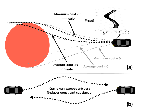
Figure 1: (a) The average cost of a trajectory does not imply safety (i.e., low maximum cost). Standard reachability methods can solve for an explicit safety boundary where max cost is zero (plot shown above the vehicle). (b) Directly optimizing for the worst-case cost can guarantee collision-avoidance. This paper presents a scalable method for optimizing this worst-case in dynamic games.

II Background

In this section, we shall present the core mathematical foundation of our approach and the corresponding related work. We shall treat the case of dynamic games separately from that of single-player optimal control, in which reachability problems are more traditionally studied. Further, we note that although some of the prior work we reference deals in continuous-time, our methods operate in discrete-time.

II-A Multi-Player Reachability Games

We address both the multi-player and the single-player settings in this paper. A multi-player dynamic game with $N$ players evolving over discrete-time $t\in\{1,\dots,T\}\equiv[T]$ is primarily defined by its dynamics, information pattern, and cost structure.

The dynamics are specified as a difference equation, $x_{t+1}=f_{t}(x_{t},u_{t}^{1:N})$, which describes the evolution of the state $x_{t}\in\mathcal{X}_{t}\subseteq\mathbb{R}^{n}$ with each player $i$’s control input $u_{t}^{i}\in\mathcal{U}^{i}_{t}\subseteq\mathbb{R}^{m^{i}}$. For clarity, in this work we we shall presume that these constraints are trivial, i.e. that $x_{t}\in\mathbb{R}^{n},u_{t}^{i}\in\mathbb{R}^{m^{i}}$.

The information pattern or strategy space specifies what each player knows at each timestep. For our purposes, we shall presume a feedback structure in which each player knows the full state of the game $x_{t}$ and chooses a corresponding input according to their strategy, i.e., $u_{t}^{i}\equiv\gamma_{t}^{i}(x_{t}),\gamma_{t}^{i}\in\Gamma_{t}^{i}$ a measurable map from state to input for each player.

Finally, the cost structure of the game may be defined arbitrarily for each player, i.e.,

$$J^{i}(x_{1},\gamma_{1:T}^{1:N}) \equiv\mathcal{J}^{i}(\mathbf{x})$$ (1)

$$:=\max_{t\in[T]}g_{t}^{i}(x_{t})\,,$$ (2)

where we have defined $\mathbf{x}:=x_{1:T+1}$, and $g_{t}^{i}(x_{t})$ encodes an arbitrary state cost at each time (such as distance-to-collision). For clarity, we shall use maxima throughout the paper, although minima may also be used. We shall use the shorthand $\gamma^{i}\equiv\gamma_{1:T}^{i}$ to represent each player’s strategy over time. Additionally, note that player $i$’s cost function $J^{i}$ explicitly depends upon the initial condition $x_{1}$ which determines the entire game trajectory $\mathbf{x}$. Further, note that we have presumed control-independence to restrict our attention to state reachability problems. For a much more detailed introduction to dynamic game theory, please refer to [1] and for their initial conception [2, 3].

Before proceeding, we note several important assumptions inherent to this formulation. First, we have presumed a known, finite time interval over which the game takes place. Although this common assumption [1] appears to neglect a wide class of long-horizon and infinite-horizon problems, such issues are often practically addressed in optimal control settings via repeated solutions in a receding time horizon, e.g., [4]. Second, we have presumed that all players observe the full state of the game $x_{t}$. Indeed, this is a strong assumption, especially in games with many players. Nevertheless, we assume full state feedback because it yields computationally-efficient solution methods such as [5, 6] and allows strategies to depend upon current information rather than only initial conditions as in other recent methods for solving smooth general-sum dynamic games [7, 8]. Partial observations are also possible in principle, but no efficient computational methods are known for this more general case. In the stochastic setting, however, recent results have shown promise [9].

As in classical discrete games, smooth dynamic games admit a variety of solution concepts. We shall consider the well-known Nash equilibrium concept, in which we seek a set of strategies for all players, $\gamma^{1:N,*}$, where no player has a unilateral incentive to deviate from its strategy, i.e.

Definition 1

(Nash Equilibrium, see e.g. [1, Chapter 6]) A set of strategies $\gamma^{1:N,*}$ is a Nash equilibrium if

$$J^{i}\big{(}x_{1},\gamma^{1:N,*}\big{)}\leq J^{i}\big{(}x_{1},\gamma^{i},\gamma^{-i*}\big{)},\forall i\in[N],\forall\gamma_{t}^{i}\in\Gamma_{t}^{i}\,,\vspace{-0.2cm}$$

where by $\gamma^{-i*}$ we denote the Nash strategies of all players other than $i$.

Assumption 1

We shall presume the existence of a Nash equilibrium in the feedback strategies $\{\gamma^{i}\}$. Conditions under which this is guaranteed are detailed in [1, Chapter 6], but as a practical matter it is often possible to construct continuous dynamic games in which equilibria exist.

We note that, in a single-player optimal control setting where $N=1$, a Nash equilibrium is precisely a globally optimal strategy. In this sense then, the method we develop for dynamic games also applies to optimal control problems. Since the single-player case is extremely well studied in its own right—and especially in the context of reachability—we present it separately.

II-B Single-Player Setting

In the single-player case, our work can be understood as an approximate method for finding optimal trajectories for a class of Hamilton-Jacobi reachability problems [10, 11]. More precisely, we are concerned with choosing a discrete-time control signal which minimizes the extremum of a target function over time, and as before we restrict our attention to maxima although our contributions also apply for minima. As described above and illustrated in Fig. 1 this problem structure can be used to encode safety constraints.

These problems are characterized by dynamics and cost structure. The dynamics describe the evolution of the state variable $x_{t}\in\mathcal{X}_{t}\subseteq\mathbb{R}^{n}$ with control variable $u_{t}\in\mathcal{U}_{t}\subseteq\mathbb{R}^{m}$ as $x_{t+1}=f_{t}(x_{t},u_{t}),\forall t\in[T-1]$. The cost structure and resulting optimal control problem are as follows:

$$\mathbf{x}^{*},\mathbf{u}^{*}=\arg\min_{\mathbf{x},\mathbf{u}} \Big{[}J(\hat{x}_{1})=\max_{t\in[T]}~{}g_{t}(x_{t})\Big{]}$$ (3)

such that $$u_{t}\in\mathcal{U}_{t},\forall t\in[T]\,,$$

$$x_{t}\in\mathcal{X}_{t},\forall t\in[T]\,,$$

$$x_{t+1}=f_{t}(x_{t},u_{t}),\forall t\in[T-1]\,,$$

$$x_{1}=\hat{x}_{1}~{}\textnormal{(given initial state)}.$$

with optimal trajectory given by $(\mathbf{x}^{*},\mathbf{u}^{*})$. Note that we use shorthand $\mathbf{x}:=x_{1:T},\mathbf{u}:=u_{1:T}$ (in the multi-player context, we denote $\mathbf{u}^{1:N}\equiv u_{1:T}^{1:N}$).

Assumption 2

We shall presume that feasible solutions always exist in (3). This assumption virtually always satisfied, e.g., if $\mathcal{U}_{t}$ is nonempty and $\mathcal{X}_{t}$ is sufficiently large.

This type of problem has been studied extensively in the literature. Broadly, approaches fall into three categories. (a) Conservative, often geometric, methods approximate the reachable set which (depending upon the type of extremum) contains states from which either every or at least one trajectory ends in a given target set; examples include [12, 13]. (b) Approximate dynamic programming methods (e.g., [14, 15]) attempt to find a parameterized “value” function which summarizes the cost-to-go from any state. (c) Finally, grid-based Hamilton-Jacobi methods are one such method (summarized in [16]), in which the value function is represented on a lattice. While resolution-complete, these methods suffer from Bellman’s “curse of dimensionality” [17] and do not generally scale to high-dimensional problems.

Local methods for solving (3) are also possible. In the common setting of time-additive costs, gradient-based methods are both commonly-used and well-understood [4]. However, to the best of our knowledge gradient methods are not used for reachability problems with extrema-over-time objectives. We show in Sec. IV that, when applied in the single-player setting, our method for multi-player games reduces to just such a method. Further, we show that a wide variety of other existing methods [18, 19] may also be used in this case, thereby facilitating the further investigation of reachability methods in high-dimensional problems.

III Approximately Optimal Trajectories for Multi-Agent Reachability

In this section, we consider an $N$-player dynamic game with maximum-over-time cost structure as in (2), in which each player wishes to minimize this same form of objective, though now with different instantaneous costs $g^{i}$ for each player $i\in[N]$. Note that our approach also applies when some players instead have minimum-over-time or even sum-over-time objectives.

III-A Algorithmic Overview

In practice, it is generally intractable to compute Nash equilibria [20]. Instead, we settle for “approximate local” feedback Nash equilibria. These solutions are “local” in the sense that they only attempt to satisfy Def. 1 within a small neighborhood in the strategy space [21], and “approximate” in the sense that they may still be a small distance $\delta$ from a local Nash equilibrium [1]. However, making these relaxations facilitates a much more computationally tractable algorithm for finding solutions—the iterative linear-quadratic (ILQ) method of [5].

This approach is similar to the ILQ regulator [22, 23, 24, 25] and differential dynamic programming [26, 27], and generalizes the two-player zero-sum approach of [28]. Furthermore, it is worthwhile to note that the approach of [5] finds approximate feedback Nash solutions, which differ from the open-loop Nash solutions found in, e.g., [8, 7]. Still, the quadratic approximation of cost developed in Sec. III-B is also compatible with open-loop methods [8, 7].

For brevity, we omit a full description of the ILQ algorithm and direct the reader to [5, Algorithm 1]. In short, however, the method iteratively refines strategies for all players using a closed form solution to a sequence of subproblems. Each of these subproblems is formed by taking a linear approximation of game dynamics $f_{t}$ and a quadratic approximation of each player’s running cost $g^{i}_{t}$. In [5], it is assumed that costs in these subproblems are time-additive; in this paper, we generalize to the case of extrema-over-time objectives found in reachability problems.

III-B Quadratic Approximation

The ILQ game approach of [5] relies upon an efficient computation of the global feedback Nash equilibrium of a linear-quadratic game. Such an efficient solution is only known for games with sum-over-time structure [1, 29], not maximum-over-time problems as in (2). To approximate a maximum-over-time cost structure in a sum-over-time form, we recognize that, at each iteration of the overall ILQ algorithm, a quadratic approximation to the maximum-over-time objective is entirely determined by the time at which maximum cost is achieved, i.e. $t={t^{\prime}}$. We consider variations $x_{t^{\prime}}=\bar{x}_{t^{\prime}}+h$ about state trajectory $\bar{\mathbf{x}}:=\bar{x}_{1:T}$ and presume that $g_{t}^{i}(x_{t})<g_{t^{\prime}}^{i}(x_{t^{\prime}}),\forall t\neq{t^{\prime}}$, which holds in nondegenerate cases. Thus equipped, we may form a Taylor expansion of the overall objective for player $i$ as

$$\mathcal{J}^{i}(\mathbf{x})\approx g_{t^{\prime}}^{i}(\bar{x}_{t^{\prime}})+\frac{1}{2}\big{(}2q_{t^{\prime}}^{iT}+h^{T}Q_{t^{\prime}}\big{)}h\,,$$ (4)

where $q_{t^{\prime}}^{i}:=\nabla_{x}g^{i}_{t^{\prime}}(\bar{x}_{t^{\prime}})$ and $Q_{t^{\prime}}^{i}:=\nabla^{2}_{x}g^{i}_{t^{\prime}}(\bar{x}_{t^{\prime}})$. Other terms in the expansion do not appear because, at $\bar{\mathbf{x}}$, overall cost $\mathcal{J}^{i}(\bar{\mathbf{x}})=\max_{t\in[T]}g^{i}_{t}(\bar{x}_{t})=g_{t^{\prime}}^{i}(\bar{x}_{t^{\prime}})$. This implies that cost derivatives at other times (i.e., $q^{i}_{t},Q^{i}_{t},t\neq{t^{\prime}}$) are identically zero.

Thus, (4) constitutes a second-order Taylor expansion of player $i$’s maximum-over-time objective. This quadratic approximation is trivially expressible as a sum-over-time in which all terms where $t\neq{t^{\prime}}$ are zero. Hence, it is compatible with the ILQ game algorithm from [5]. As in the sum-over-time setting, this algorithm identifies approximate, local feedback Nash equilibria.

III-C Relaxation

Before applying the ILQ game method from [5, Algorithm 1], we must ensure that solutions to the LQ game subproblems it solves at each iteration are well-defined. In state reachability games (2), each player’s objective does not depend upon its control input $u_{t}^{i}$. However, analytical Nash solutions to LQ games require such dependence [1, Chapter 6]; hence, we must also incorporate control dependence in each player’s objective. That is, we must further approximate the instantaneous cost $g_{t}^{i}(x_{t})$ by adding a small but nonzero dependence upon control $u_{t}^{1:N}$. Concretely, we approximate each player’s objective at level $\epsilon>0$ as follows:

$$\tilde{\mathcal{J}}^{i}_{\epsilon}(x_{1:T},u_{1:T}^{1:N}) =\max_{t\in[T]}~{}\tilde{g}_{t,\epsilon}^{i}$$

$$=\max_{t\in[T]}\left\{g_{t}^{i}(x_{t})+\frac{1}{2}\epsilon\|u_{t}^{i}\|_{2}^{2}\right\}\,.$$ (5)

As we take $\epsilon\to 0$, we recover the original problem under moderate assumptions.

Assumption 3

Nash strategies for games with costs as in both (2) and (5) exist and are feasible, for all positive $\epsilon$.

Assumption 4

Limiting Nash strategies exist for the game with cost (5) as $\epsilon\to 0$ and are feasible.

Theorem 1

If $\gamma^{1:N,*}$ are Nash strategies in the limit $\epsilon\to 0$ for the game with relaxed objective (5), then they are also Nash strategies in the original game with each players’ cost as in (2).

Proof:

We rewrite player $i$’s problem in the original game with costs (2) as

$$\gamma^{i*}=\arg\min_{\gamma^{i}}\max_{t\in[T]}g_{t}^{i}(x_{t}) =\arg\min_{\gamma^{i}}\lim_{\epsilon\to 0}\max_{t}~{}\tilde{g}_{t,\epsilon}^{i}$$

$$=\lim_{\epsilon\to 0}\arg\min_{\gamma^{i}}\max_{t}~{}\tilde{g}_{t,\epsilon}^{i}=\gamma^{i*}\,,$$

where we can interchange the limit and minimum safely by Assumptions 3 and 4.

Thus, if these assumptions hold, the limiting Nash strategies in the relaxed game (5) are Nash in the original game with player costs from (2). ∎

Remark 1

We note that care must be taken in the context of zero-sum games. Here, each LQ subproblem of [5, Algorithm 1] is especially susceptible to poor numerical conditioning due to the inherent adversarial competition of these games. Although these issues may be addressed with further regularization, we do not treat them here. Control constraints $u^{i}_{t}\in\mathcal{U}^{i}_{t}$ are often necessary in such settings; such constraints are neglected in this work but may be addressed using penalty and interior point methods.

III-D Example: Three-Player Avoidance Game

Here and in Sec. III-E we demonstrate our method in operation. As our method is the first to treat $N$-player general reachability games, a direct comparison to prior work is not possible.

Consider a three-player dynamic game where each player has bicycle dynamics, i.e.

$$\dot{x}^{i}=\frac{d}{dt}\begin{bmatrix}p_{x}^{i}\\ p_{y}^{i}\\ \theta^{i}\\ \phi^{i}\\ v^{i}\end{bmatrix}=\begin{bmatrix}v^{i}\cos(\theta^{i})\\ v^{i}\sin(\theta^{i})\\ v^{i}\tan(\phi^{i})/L^{i}\\ \omega^{i}\\ \alpha^{i}\end{bmatrix}\,.$$ (6)

Here, player $i$’s input $u^{i}=(\omega^{i},\alpha^{i})$ controls the front wheel angular rate ($\dot{\phi}^{i}$) and linear acceleration ($\dot{v}^{i}$), respectively. Each bicycle has inter-axle distance $L^{i}>0$, which enforces a minimum positive turning radius.

We construct a dynamic game in which each player has Euler-discretized dynamics according to (6) with a sampling time of $0.1\text{\,}\mathrm{s}$ and time horizon $2\text{\,}\mathrm{s}$ (used throughout), and the following cost structure (written for player 1 for brevity), which penalizes player 1 for the smallest relative distance between it and players 2 and 3:

$$g_{t}^{1}=\bar{d}-\min\{ d_{t}^{12},~{}d_{t}^{13}\},$$ (7)

$$\textnormal{where}~{}d_{t}^{12} :=\|(p_{x,t}^{1},p_{y,t}^{1})-(p_{x,t}^{2},p_{y,t}^{2})\|_{2}\,,$$

$$d_{t}^{13} :=\|(p_{x,t}^{1},p_{y,t}^{1})-(p_{x,t}^{3},p_{y,t}^{3})\|_{2}\,,$$

and define $\tilde{g}_{t,\epsilon}^{i}$ as in (5). Here, $\bar{d}$ is a desired separation between the vehicles.

We plot the approximately optimal strategies for the relaxed game constructed according to (5) in Fig. 2, showing the affect of decreasing $\epsilon\to 0$. As we approach this limit, the players take more extreme avoidance maneuvers. Additionally, for each $\epsilon$ our method finds a solution reliably in real-time under $1\text{\,}\mathrm{s}$.

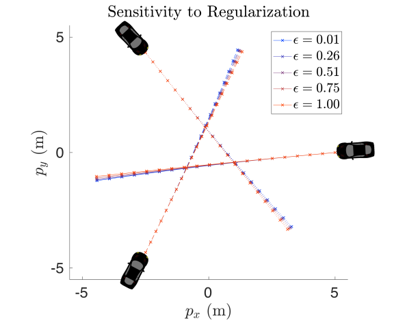
Figure 2: Optimal trajectories in the three-player avoidance game for varying $\epsilon$ (black cars mark the initial position for each player). As $\epsilon\to 0$ the more blue trajectories display a greater tendency toward avoidance.

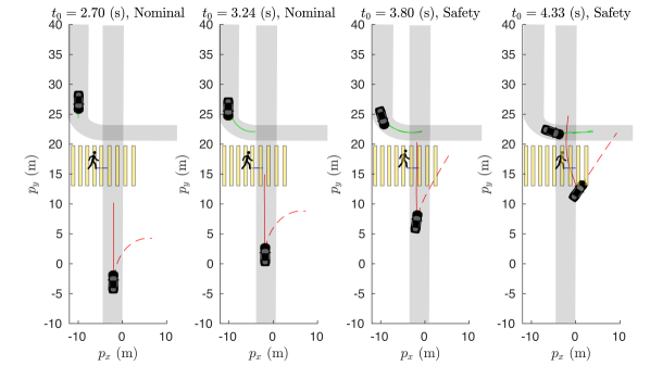
Figure 3: Optimal trajectories in the intersection game, executed with a receding time horizon. Solid lines indicate nominal trajectories. Dashed lines are safe trajectories for the ego vehicle, which successfully avoids collision by following a minimally-invasive control strategy.

III-E Example: Receding Horizon, Minimally-Invasive Control

Perhaps the most practical usage of reachability-based controllers is in receding horizon and minimally-invasive settings, where a single “ego” agent overrides its nominal controller whenever safety is nearly violated. In receding horizon problems, players’ strategies at time $t$ only match those for the most recently solved game, not earlier ones; hence, collision-avoidance is not generally guaranteed. For a recent analysis of the induced information structure, please refer to [30]. Fig. 3 demonstrates our method’s operation in a receding horizon, minimally-invasive setting for a three-player intersection game resembling that in [5].

Here, the ego vehicle (at bottom, red trajectory) and another car (both system dynamics are as above) navigate an intersection while a pedestrian crosses a crosswalk (its dynamics are those of a standard planar unicycle model). We set up costs for a nominal game as in [5], and in order to emphasize the role of a safety controller, we reduce the cost weight for maintaining sufficient proximity between agents. We also construct an identical reachability game to encode collision-avoidance, in which the ego vehicle’s objective is of the form (7), and its equilibrium trajectory is shown in dotted red. Note that it avoids proximity to a much greater degree (i.e., behaves much more conservatively) than the nominal strategy; this is typical of safety strategies. As shown in Fig. 3, over time the ego vehicle switches to the safety strategy as its planned (nominal) trajectory nears other agents. Time $t_{0}$ refers to the time of each planning invocation of horizon $T=$2\text{\,}\mathrm{s}$$. As above, our method operates in real-time, and since each receding-horizon invocation can be warm-started with the previous solution the amortized speed per invocation is typically on the order of $0.1\text{\,}\mathrm{s}$ or less.

Computation of a Nash solution is centralized rather than distributed among all agents. As in robust planning methods, e.g. [31], we envision such computation constituting the motion planning process for a single ego vehicle. Here, the reachability game formulation allows the ego vehicle to reason about how other vehicles may react to its own control decisions and thereby allow it to find interactive solutions in multi-agent settings.

IV Approximate Optimal Trajectories for Single-Agent Reachability

The single-player reachability problem (3) is already in the form of a nonconvex, nonlinear program. In this case, our approach from Sec. III may be viewed as a direct adaptation of well-known ILQ regulator of [22, 23, 24, 25] to the setting of state reachability. However, a wider variety of methods for approximately solving general nonlinear programming problems can be found, e.g., in [18, 19]. Here, solution methods are approximate in the sense that they find local optima. Due to this approximation, solutions are conservative as discussed below.

Theorem 2

Define optimal cost or value $V(\hat{x}_{1})$ as the globally minimum cost $J^{*}(\hat{x}_{1})$ attained by (3) at initial state $\hat{x}_{1}$, and $\tilde{V}(\hat{x}_{1})$ a local minimum identified by a particular nonlinear programming algorithm. For any scalar threshold $\alpha\in\mathbb{R}$, the following inequalities hold:

$$J^{*}(\hat{x}_{1})\equiv V(\hat{x}_{1}) \leq\tilde{V}(\hat{x}_{1})\,,~{}\textnormal{and}$$ (8)

$$\{\hat{x}_{1}:V(\hat{x}_{1})\leq\alpha\} \subseteq\{\hat{x}_{1}:\tilde{V}(\hat{x}_{1})\leq\alpha\},~{}\forall\hat{x}_{1}\in\mathcal{X}_{1}\,.$$ (9)

Sublevel sets of this form are called reachable sets and these inequalities imply that the solution is conservative, i.e., any state it concludes is safe (with sufficiently small cost) would also be safe for the globally optimal controller.

Proof:

The first inequality is a consequence of the local optimality of solutions to nonconvex programming, and the second inequality follows from the first. ∎

Further, in the special case in which (3) is convex, we have the following result.

Theorem 3

Define $V$ and $\tilde{V}$ as before, and suppose that problem (3) is convex in the decision variables, i.e., that sets $\mathcal{X}_{t},\mathcal{U}_{t}$ are convex for all $t$, dynamics $f$ are affine in $x_{t},u_{t}$ for all $t$, and instantaneous cost $g_{t}$ is a convex function of its argument (and that the cost has a maximum-over-time structure). Then, the local minimum cost $\tilde{V}$ is equivalent to the globally minimal $V$.

Proof:

Follows from the global optimality of solutions to convex programs. ∎

Our main algorithmic contribution treats the multi-player noncooperative game setting. While our method applies in this single-player setting, to demonstrate the general utility of posing single-player reachability problems as nonlinear programs we utilize existing, off-the-shelf methods instead. That is, by resorting to local methods for nonlinear programming, solution methods may be significantly more computationally efficient than global techniques such as [10, 13]. More to the point, to our knowledge, these methods are not widely used in the reachability literature and have the potential to dramatically improve practical performance in realistic, high-dimensional cases.

IV-A Example: High-Dimensional Quadrotor

To demonstrate the computational advantages of local solutions for single-player reachability problems, we construct a high-dimensional quadrotor example with a 14-dimensional state space. The continuous-time dynamics are given below and may be found in [32]:

$$x =(p_{x},p_{y},p_{z},\psi,\theta,\phi,v_{x},v_{y},v_{z},\zeta,\xi,p,q,r)$$

$$\frac{d}{dt} \begin{bmatrix}p_{x}\\ p_{y}\\ p_{z}\\ \psi\\ \theta\\ \phi\\ v_{x}\end{bmatrix}=\begin{bmatrix}v_{x}\\ v_{y}\\ v_{z}\\ q\\ r\\ p\\ g_{x}\zeta\end{bmatrix},~{}\frac{d}{dt}\begin{bmatrix}v_{y}\\ v_{z}\\ \zeta\\ \xi\\ p\\ q\\ r\end{bmatrix}=\begin{bmatrix}g_{y}\zeta\\ g_{z}\zeta-g\\ \xi\\ \tau\\ \alpha_{x}/I_{x}\\ \alpha_{y}/I_{y}\\ \alpha_{z}/I_{z}\end{bmatrix},$$ (10)

$$\textnormal{with}~{}g_{x} =(\sin(\phi)\sin(\psi)+\cos(\phi)\cos(\psi)\sin(\theta))/m,$$

$$g_{y} =(\cos(\phi)\sin(\psi)\sin(\theta)-\cos(\psi)\sin(\phi))/m,$$

$$g_{z} =\cos(\phi)\cos(\theta)/m\,,$$

where $g=$9.81\text{\,}\mathrm{m}\text{\,}{\mathrm{s}}^{-2}$$ is the acceleration due to gravity. Here, $(m,I_{x},I_{y},I_{z})$ are mass and inertia parameters (in our example, set to unity), and the states include positions, angles, their derivatives, and a double integrator on thrust. The controls are the second-derivative of thrust ($\tau$), and angular accelerations $(\alpha_{x},\alpha_{y},\alpha_{z})$. As before, we use an Euler discretization.

The instantaneous cost records the signed distance from the boundary of a cube, i.e. $g(x)=\|(p_{x},p_{y},p_{z})\|_{\infty}-B$. Marking the boundary of the unsafe region in which $g>0$ in red, Fig. 4 displays the approximately optimal trajectory. To emphasize the generality of the nonlinear programming formulation and the quality of existing solution methods in this single-player context, we use well-known existing tools such as IPOPT [33] and SNOPT [34, 35], accessed via YALMIP [36] in MATLAB^®.

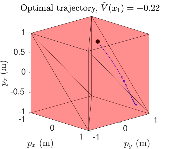
Figure 4: Locally optimal trajectory for high-dimensional quadrotor. The boundary of the unsafe region where $g>0$ is shown in red. The solid black dot denotes the quadrotor’s initial position.

V Discussion

This paper presents a novel approach to solving extremum-over-time $N$-player reachability games. Our method is computationally tractable and yields real-time approximate solutions to high-dimensional problems. In the game setting, we introduce an arbitrarily accurate relaxation of the original objective structure and provide a guarantee of limiting convergence, and in the single-player optimal control setting, we provide a conservativeness guarantee. We have demonstrated our approach in several examples, including a three-player dynamic game, a receding horizon traffic example, and a high-dimensional quadrotor example. In the remainder of this section, we shall outline promising extensions and directions for future work.

V-A Numerical Stability

The choice of $\epsilon$ may have significant impact upon the numerical stability of the ILQ algorithm, since the underlying LQ feedback Nash solution relies upon solving linear systems of equations which become singular when $\epsilon\approx 0$. Further work is needed to improve numerical stability in these cases.

V-B Constraints

A related, promising direction is the incorporation of constraints on both states and inputs. Constrained games require a distinct notion of equilibrium, such as that of generalized Nash equilibria. Our current work investigates efficient methods for solving these types of feedback games, although it is worth noting that solutions already exist for the simpler open-loop information pattern [7].

V-C Annealing

Although we have not investigated it in this work, we believe that annealing $\epsilon\to 0$ may improve asymptotic approximation quality. Such annealing may encourage the iterative ILQ method of Sec. III-A to find globally optimal solutions of the original reachability problem. We note that, because each subproblem with fixed $\epsilon$ may be solved so rapidly, the computational burden of annealing is minimal.

References

- [1] Tamer Başar and Geert Jan Olsder “Dynamic noncooperative game theory” SIAM, 1999
- [2] R Isaacs “Differential games, parts 1-4” In The Rand Corpration, Research Memorandums Nos. RM-1391, RM-1411, RM-1486 55, 1954
- [3] Rufus Isaacs “Differential games: a mathematical theory with applications to warfare and pursuit, control and optimization” Courier Corporation, 1999
- [4] Francesco Borrelli, Alberto Bemporad and Manfred Morari “Predictive control for linear and hybrid systems” Cambridge University Press, 2017
- [5] David Fridovich-Keil, Ellis Ratner, Anca D Dragan and Claire J Tomlin “Efficient Iterative Linear-Quadratic Approximations for Nonlinear Multi-Player General-Sum Differential Games” In arXiv preprint arXiv:1909.04694, 2019
- [6] David Fridovich-Keil, Vicenç Rubies-Royo and Claire J Tomlin “An Iterative Quadratic Method for General-Sum Differential Games with Feedback Linearizable Dynamics” In arXiv preprint arXiv:1910.00681, 2019
- [7] Simon Le Cleac’h, Mac Schwager and Zachary Manchester “ALGAMES: A Fast Solver for Constrained Dynamic Games” In arXiv preprint arXiv:1910.09713, 2019
- [8] Bolei Di and Andrew Lamperski “Newton’s Method and Differential Dynamic Programming for Unconstrained Nonlinear Dynamic Games” In 2019 IEEE 58th Conference on Decision and Control (CDC), 2019, pp. 4073–4078 IEEE
- [9] Wilko Schwarting, Alyssa Pierson, Sertac Karaman and Daniela Rus “Stochastic Dynamic Games in Belief Space” In arXiv preprint arXiv:1909.06963, 2019
- [10] Ian M Mitchell, Alexandre M Bayen and Claire J Tomlin “A time-dependent Hamilton-Jacobi formulation of reachable sets for continuous dynamic games” In IEEE Transactions on automatic control 50.7 IEEE, 2005, pp. 947–957
- [11] Jaime F Fisac, Mo Chen, Claire J Tomlin and S Shankar Sastry “Reach-avoid problems with time-varying dynamics, targets and constraints” In Proceedings of the 18th international conference on hybrid systems: computation and control, 2015, pp. 11–20
- [12] Matthias Althoff and Bruce H Krogh “Zonotope bundles for the efficient computation of reachable sets” In 2011 50th IEEE conference on decision and control and European control conference, 2011, pp. 6814–6821 IEEE
- [13] Anirudha Majumdar, Ram Vasudevan, Mark M Tobenkin and Russ Tedrake “Convex optimization of nonlinear feedback controllers via occupation measures” In The International Journal of Robotics Research 33.9 SAGE Publications Sage UK: London, England, 2014, pp. 1209–1230
- [14] Dimitri P Bertsekas “Approximate dynamic programming” Athena scientific Belmont, 2012
- [15] Dimitri P Bertsekas and John N Tsitsiklis “Neuro-dynamic programming” Athena Scientific, 1996
- [16] Somil Bansal, Mo Chen, Sylvia Herbert and Claire J Tomlin “Hamilton-Jacobi reachability: A brief overview and recent advances” In 2017 IEEE 56th Annual Conference on Decision and Control (CDC), 2017, pp. 2242–2253 IEEE
- [17] Richard Bellman “Dynamic programming”, 1956
- [18] Dimitri P Bertsekas “Nonlinear programming” In Journal of the Operational Research Society 48.3 Taylor & Francis, 1997, pp. 334–334
- [19] Jorge Nocedal and Stephen Wright “Numerical optimization” Springer Science & Business Media, 2006
- [20] Christos H Papadimitriou “The complexity of finding Nash equilibria” In Algorithmic game theory 2 Cambridge Univ. Press Cambridge, 2007, pp. 30
- [21] Lillian J Ratliff, Samuel A Burden and S Shankar Sastry “On the characterization of local Nash equilibria in continuous games” In Transactions on Automatic Control 61.8 IEEE, 2016, pp. 2301–2307
- [22] Weiwei Li and Emanuel Todorov “Iterative linear quadratic regulator design for nonlinear biological movement systems.” In ICINCO, 2004, pp. 222–229
- [23] Emanuel Todorov and Weiwei Li “A generalized iterative LQG method for locally-optimal feedback control of constrained nonlinear stochastic systems” In American Control Conference (ACC), 2005, pp. 300–306 IEEE
- [24] Jur Berg “Iterated LQR smoothing for locally-optimal feedback control of systems with non-linear dynamics and non-quadratic cost” In American Control Conference (ACC), 2014, pp. 1912–1918 IEEE
- [25] Jianyu Chen, Wei Zhan and Masayoshi Tomizuka “Constrained iterative LQR for on-road autonomous driving motion planning” In International Conference on Intelligent Transportation Systems (ITSC), 2017, pp. 1–7 IEEE
- [26] David Mayne “A second-order gradient method for determining optimal trajectories of non-linear discrete-time systems” In International Journal of Control 3.1 Taylor & Francis, 1966, pp. 85–95
- [27] David Jacobson and David Mayne “Differential Dynamic Programming”, Modern analytic and computational methods in science and mathematics American Elsevier Publishing Company, 1970
- [28] H Mukai et al. “Sequential linear quadratic method for differential games” In Proc. 2nd DARPA-JFACC Symposium on Advances in Enterprise Control, 2000, pp. 159–168 Citeseer
- [29] Alan Wilbor Starr and Yu-Chi Ho “Nonzero-sum differential games” In Journal of optimization theory and applications 3.3 Springer, 1969, pp. 184–206
- [30] Ovanes Petrosian and Anna Tur “Hamilton-Jacobi-Bellman Equations for Non-cooperative Differential Games with Continuous Updating” In International Conference on Mathematical Optimization Theory and Operations Research, 2019, pp. 178–191 Springer
- [31] Jason Hardy and Mark Campbell “Contingency planning over probabilistic obstacle predictions for autonomous road vehicles” In IEEE Transactions on Robotics 29.4 IEEE, 2013, pp. 913–929
- [32] Saif A Al-Hiddabi “Quadrotor control using feedback linearization with dynamic extension” In 2009 6th International Symposium on Mechatronics and its Applications, 2009, pp. 1–3 IEEE
- [33] A Wächter and L T Biegler “On the Implementation of a Primal-Dual Interior Point Filter Line Search Algorithm for Large-Scale Nonlinear Programming” In Mathematical Programming 106.1, 2006, pp. 25–57
- [34] Philip E. Gill, Walter Murray and Michael A. Saunders “SNOPT: An SQP algorithm for large-scale constrained optimization” In SIAM Rev. 47, 2005, pp. 99–131
- [35] Philip E. Gill, Walter Murray, Michael A. Saunders and Elizabeth Wong “User’s Guide for SNOPT 7.7: Software for Large-Scale Nonlinear Programming”, 2018
- [36] J. Löfberg “YALMIP : A Toolbox for Modeling and Optimization in MATLAB” In In Proceedings of the CACSD Conference, 2004