Random Fourier Features based SLAM

Abstract

This work is dedicated to simultaneous continuous-time trajectory estimation and mapping based on Gaussian Processes (GP). State-of-the-art GP-based models for Simultaneous Localization and Mapping (SLAM) are computationally efficient but can only be used with a restricted class of kernel functions. This paper provides the algorithm based on GP with Random Fourier Features (RFF) approximation for SLAM without any constraints. The advantages of RFF for continuous-time SLAM are that we can consider a broader class of kernels and, at the same time, maintain computational complexity at reasonably low level by operating in the Fourier space of features. The accuracy-speed trade-off can be controlled by the number of features. Our experimental results on synthetic and real-world benchmarks demonstrate the cases in which our approach provides better results compared to the current state-of-the-art.

I INTRODUCTION

Since the last century, probabilistic state estimation has been a core topic in mobile robotics, often as part of the problem of simultaneous localization and mapping [1, 2]. Recovery of a robot’s position and a map of its environment from sensor data is a complicated problem due to both map and trajectory are unknown as well as the correspondences between observations and landmarks [3].

The field of discrete time trajectory estimation and mapping methods is well developed [4, 5, 6, 7, 8, 9, 10, 11]. However, discrete-time representations are constrained because they are not easily adapted to irregularly distributed poses or asynchronous measurements over trajectories. In the time-continuous problem statement, the robot trajectory is a function $\bm{x}(t)$ which corresponds to a robot state at every time $t$. Simultaneous trajectory estimation and mapping (STEAM) presents the problem of estimating this function along with landmark positions [12, 13]. In the work [14] they formally derive a continuous-time SLAM problem and demonstrate the use of a parametric solution for atypical SLAM calibration problems. The use of cubic splines to parameterize the robot trajectory can also be seen in the estimation schemes in [15, 16, 17]. In the work [18] the parametric state representation was proposed due to practicality and effectiveness. The advantages of this method are that they can precisely model and interpolate asynchronous data to recover a trajectory and estimate landmark positions. The disadvantages of that algorithm are that it requires batch updates and considerable computational problems. In the work [19], the critical update to increase the efficiency of existing GP approach to solve the STEAM problem was introduced. It combines benefits of graph-based SLAM [6] and GP-based solution [20] to provide a computationally efficient solution to the STEAM problem even for large datasets. However, the computational efficiency comes at the cost of constrained class of kernel functions. They use state-space formulation of GP model. Fast inference in this case is possible if we impose Markovian structure on the trajectory: it is supposed that two points on the trajectory are conditionally independent given all other points if these two points are not neighboring. However, in some cases the accuracy of the trajectory estimate can be increased by adjusting the estimate at the current point using all previous points in the trajectory, especially when the observations contain a considerable amount of noise.

In recent years a lot of effort has been put to develop large-scale GP models without any constraints on the kernel function [21, 22, 23]. There are two main approaches to scale up the GP model. The first one is based on Nyström approximation [24]. The idea is to approximate the kernel function using a finite set of basis functions that are based on eigenvectors of the kernel matrix. This approach is data-dependent and needs updating the basis function when new observations arrive. Another set of methods is based on Random Fourier Features (RFF) [25]. In these approaches the basis functions depend solely on the kernel function and independent of the data set. It provides additional computational benefits and is more attractive for SLAM problems.

The contributions of this paper are as follows. We develop random features-based SLAM approach. It uses a low-rank approximation of the kernel matrix which is dense and, therefore, does not assume the conditional independence of the points on the trajectory. We show that in certain situations removing the independence constraint allows to improve the quality of trajectory estimation. Also, low-rank structure of the approximation allows to maintain the computational complexity at reasonably low level.

The paper is organized as follows. Section II provides background on Gaussian Processes and random features-based approximation. In Section III-A we describe the proposed RFF-based SLAM. Section IV contains experimental results demonstrating how the method works in practice in comparison with the competing approach. Finally, Section V concludes the paper.

II GAUSSIAN PROCESSES

One of the most efficient tools for approximating smooth functions is the Gaussian Process (GP) Regression [26, 27]. GP regression is a Bayesian approach where a prior distribution over functions is assumed to be a Gaussian Process, i.e. $y=f(\bm{x})+\varepsilon$ with $f\sim\mathcal{GP}(\mu(\bm{x}),k(\bm{x},\bm{x}^{\prime}))$ and white noise $\varepsilon\sim\mathcal{N}(0,\sigma^{2}_{noise})$, so that

$$\mathbf{y}\,|\,\mathbf{X}\sim\mathcal{N}(\bm{\mu},\,\mathbf{K}_{f}+\sigma_{noise}^{2}\mathbf{I}),$$

where $\mathbf{y}=(y_{1},y_{2},\ldots,y_{N})$ is a vector of outputs, $\bm{X}=(\bm{x}_{1}^{\top},\bm{x}_{2}^{\top},\ldots,\bm{x}_{N}^{\top})^{\top}$ is a matrix of inputs, $\bm{x}_{i}\in\mathbb{R}^{d}$, $\sigma_{noise}^{2}$ is a noise variance, $\bm{\mu}=(\mu(\bm{x}_{1}),\mu(\bm{x}_{2}),\ldots,\mu(\bm{x}_{N}))$ is a mean vector modeled by some function $\mu(\bm{x})$, $\mathbf{K}_{f}=\{k(\bm{x}_{i},\bm{x}_{j})\}_{i,j=1}^{N}$ is a covariance matrix for some a priori selected covariance function $k$ and $\mathbf{I}$ is an identity matrix. An example of such a function is a Radial Basis Function (RBF) kernel

$$k(\bm{x},\bm{x}^{\prime})=\exp\left(-\frac{1}{2}\sum_{i=1}^{d}\left(\frac{\bm{x}^{(i)}-\bm{x}^{\prime}{}^{(i)}}{\sigma_{i}}\right)^{2}\right),$$

where $\sigma_{i},i=1,\ldots,d$ are parameters of the kernel (hyperparameters of the GP model) and $\bm{x}^{(i)}$ is an $i$-th element of vector $\bm{x}$. The hyperparameters should be chosen according to the given data set.

For a new unseen data point $\bm{x}_{*}$ the conditional distribution of $f(\bm{x})$ given $(\bm{y},\bm{X})$ is equal to

$$\begin{gathered}\hat{f}(\bm{x}_{*})\sim\mathcal{N}\left(\hat{\mu}(\bm{x}_{*}),\hat{\sigma}^{2}(\bm{x}_{*})\right),\\ \hat{\mu}(\bm{x}_{*})=\mu(\bm{x}_{*})+\mathbf{k}(\bm{x}_{*})^{\top}\mathbf{K}^{-1}\left(\mathbf{y}-\bm{\mu}\right),\\ \hat{\sigma}^{2}(\bm{x}_{*})=k(\bm{x}_{*},\bm{x}_{*})-\mathbf{k}(\bm{x}_{*})^{\top}\mathbf{K}^{-1}\mathbf{k}(\bm{x}_{*}),\end{gathered}$$ (1)

where $\mathbf{k}(\bm{x}_{*})=(k(\bm{x}_{*},\bm{x}_{1}),\ldots,k(\bm{x}_{*},\bm{x}_{N}))^{T}$ and $\mathbf{K}=\mathbf{K}_{f}+\sigma_{noise}^{2}\mathbf{I}$.

The runtime complexity of the construction of the GP regression model is $\mathcal{O}(N^{3})$ as we need to calculate the inverse of $\mathbf{K}$.

II-A Random Fourier Features

To approach the computational complexity of building a GP model we use Random Fourier Features (RFF). The idea behind RFF is in Bochner’s theorem [28] stating that any shift-invariant kernel $k(\bm{x},\bm{y})=k^{\prime}(\bm{x-y})$ is a Fourier transform of a non-negative measure $p(\bm{w})$, i.e.

$$k^{\prime}(\bm{x-y})=\int p(\bm{w})e^{j\bm{w^{\top}(x-y)}}d\bm{w}.$$

Then the integral and, therefore, the kernel can be approximated as follows

$$k^{\prime}(\bm{x-y})\approx\phi(\bm{x})^{\top}\phi(\bm{y}),$$ (2)

where

$$\phi(\bm{x})=\sqrt{\frac{2}{D}}\begin{bmatrix}\cos(\bm{w}_{1}^{\top}\bm{x})\\ \sin(\bm{w}_{1}^{\top}\bm{x})\\ \cdots\\ \cos(\bm{w}_{D/2}^{\top}\bm{x})\\ \sin(\bm{w}_{D/2}^{\top}\bm{x})\\ \end{bmatrix},\quad\bm{w}_{j}\sim p(\bm{w}).$$ (3)

In this case the kernel matrix has a low-rank representation, $\mathbf{K}_{f}\approx\Psi\Psi^{\top}$, $\Psi=\|\phi(\bm{x}_{i})^{\top}\|_{i=1}^{N}\in\mathbb{R}^{N\times D}.$ Therefore, $\mathbf{K}^{-1}\bm{x}$ can be efficiently calculated in $\mathcal{O}(ND^{2})$ using Sherman-Morrison-Woodbury matrix identity, i.e. linearly in the number of observations. Constant $D$ — the number of features — is a hyperparameter of the algorithm, that controls the accuracy of the kernel matrix approximation. Alternatively, after we find finite-dimensional feature map that is used to approximate the kernel function as in (2), we can work in weight space view using $\phi(\bm{x})$ (see [26]). There are several approaches (e.g., [29, 23]) that both improves the quality of RFF and reduces the complexity of generating RFF to $\mathcal{O}(d\log d)$, where $d$ is the dimensionality of $\bm{x}$. Such computational complexity makes RFF a good candidate to be used for SLAM.

III SLAM

In this paper we consider the following SLAM problem. Let $\bm{l}$ be a map consisting of $L$ landmarks. Let $\mathbf{z}=\begin{bmatrix}z(t_{1})&\cdots&z(t_{N})\end{bmatrix}$ and $\mathbf{u}=\begin{bmatrix}u(t_{1})&\cdots&u(t_{N})\end{bmatrix}$ be vectors of measurements and controls at time steps $t_{1},\ldots,t_{N}$. Our goal is to estimate the posterior probability of the robot poses $\mathbf{x}=\begin{bmatrix}\bm{(}x)(t_{0})&\cdots&\bm{(}x)(t_{N})\end{bmatrix}$ and landmarks given the measurements and controls:

$$\quad p\left(\mathbf{x},\bm{l}|\mathbf{z},\mathbf{u}\right).$$ (4)

III-A RFF-SLAM

We use GP regression with RFF to estimate the state variables corresponding to trajectory and map (landmarks). Our model is as follows

$$\bm{x}(t) \sim\mathcal{GP}(\bm{\mu}_{x}(t),\bm{k}(t,t^{\prime})),$$ (5)

$$\bm{l} \sim\mathcal{N}(\bm{\mu}_{l},\mathbf{L}),$$

$$\bm{z}_{i} =\bm{h}\left(\begin{bmatrix}{\bm{x}}(t_{i})\\ {\bm{l}}\end{bmatrix}\right)+\bm{n}_{i},$$

where ${\bm{x}}(t)$ is a state of the robot at timestamp $t$, ${\bm{l}}$ is a vector of $M$ landmarks, $\bm{h}(\cdot)$ is a non-linear measurement model, $\bm{n}_{i}\sim\mathcal{N}(\bm{0},\mathbf{R}_{i})$ is measurement noise, $t_{1},\ldots,t_{N}$ is a sequence of measurement times and $(\bm{\mu}_{l},\mathbf{L})$ are prior mean and the covariance of the landmarks positions.

The paper [18] uses GP for SLAM and provides the main equations to solve the problem. We follow their approach with the difference that we utilize RFF approximation of the RBF kernel. For the RBF kernel its Fourier transform is defined by $p(\bm{w})$ being a Gaussian distribution $\mathcal{N}\left(0,\frac{1}{\sigma_{l}^{2}}\mathbf{I}\right)$. Explicit mapping (3) allows working in weight-space view

$${\bm{x}}(t)={\bm{\mu}}_{x}(t)+\begin{bmatrix}\phi_{1}(t)^{\top}{\bm{b}}_{x}^{(1)}\\ \cdots\\ \phi_{d}(t)^{\top}{\bm{b}}_{x}^{(d)}\\ \end{bmatrix}+\varepsilon,$$

where ${\bm{b}}_{x}^{(m)}\sim\mathcal{N}({\bm{\mu}}_{b}^{(m)},\mathbf{K}_{m}),m=1,\ldots,d$, $d$ is the state size, ${\bm{b}}_{x}^{(m)}\in\mathbb{R}^{D}$, $\phi_{m}({\bm{x}})$ is a feature map for the $m$-th state variable, $\mathbf{K}_{m}\in\mathbb{R}^{D\times D}$ is the prior covariance matrix of the random variable ${\bm{b}}_{x}^{(m)}$ and $\varepsilon\sim\mathcal{N}(0,\sigma^{2}\mathbf{I})$ is a Gaussian noise with variance $\sigma^{2}$. In principle, the same feature map can be used for all variables, however, it can be reasonable to use different features (corresponding to different kernels) to model different types of variables (for example, coordinates on the map and angles).

Let us denote

$$\begin{gathered}{\bm{b}}=\begin{bmatrix}{\bm{b}}_{x}^{(1)}&\cdots&{\bm{b}}_{x}^{(d)}&{\bm{l}}\end{bmatrix}^{\top},\\ {\bm{\mu}}=\begin{bmatrix}{\bm{\mu}}_{b}^{(1)}&\cdots&{\bm{\mu}}_{b}^{(d)}&{\bm{\mu}}_{l}\end{bmatrix}^{\top},\\ \mathbf{K}={\rm diag}\left(\mathbf{K}_{1},\ldots,\mathbf{K}_{d}\right),\mathbf{P}={\rm diag}\left(\mathbf{K},\mathbf{L}\right),\\ {\bm{\Phi}}_{i}={\rm diag}\left(\phi_{1}(t_{i})^{\top},\ldots,\phi_{d}(t_{i})^{\top},\mathbf{I}_{2M}\right)\\ \mathbf{R}={\rm diag}\left(\mathbf{R}_{1},\ldots,\mathbf{R}_{N}\right).\end{gathered}$$ (6)

Now to obtain both the robot states and landmarks position ${\bm{b}}$ we employ maximum a posteriori (MAP) estimate

$$p({\bm{b}}|{\bm{z}}) \propto-\frac{1}{2}\left(\sum_{i=1}^{N}\|{\bm{z}_{i}}-{\bm{h}}({\bm{\Phi}}_{i}{\bm{b}})\|_{\mathbf{R}_{i}}^{2}+\|{\bm{b}}-{\bm{\mu}}\|_{\mathbf{P}}^{2}\right)$$

$$\rightarrow\max_{{\bm{b}}}.$$ (7)

To solve the problem we do the following. Suppose, that we have an initial guess $\bar{\bm{b}}$. We update the estimate iteratively by finding the optimal perturbation vector $\delta\bm{b}^{*}$ for the linearized measurement model. Namely, we apply the first order Taylor expansion to the measurements model

$$\bm{h}({\bm{\Phi}}_{i}{\bm{b}})\approx\bm{h}({\bm{\Phi}}_{i}\bar{\bm{b}})+\mathbf{H}_{i}\delta\bm{b},\quad\mathbf{H}_{i}=\left.\frac{\partial\bm{h}({\bm{y}})}{\partial\bm{y}}\right|_{{\bm{y}}={\bm{\Phi}}_{i}\bar{\bm{b}}}.$$

Plugging linearized measurement into (III-A) we obtain the following optimization problem

$$\delta\bm{b}^{*}=\operatorname*{arg\,min}_{\delta\bm{b}}\frac{1}{2}\left(\sum_{i=1}^{N}\right. \|\bm{z}_{i}-\bm{h}({\bm{\Phi}}\bar{\bm{b}})-\mathbf{H}_{i}{\bm{\Phi}}_{i}\delta\bm{b}\|_{\mathbf{R}_{i}}^{2}$$

$$\left.+\|\bar{\bm{b}}+\delta\bm{b}-\bm{\mu}\|_{\mathbf{P}}^{2}\vphantom{\sum_{i=1}^{N}}\right).$$

The solution is given by

$$\begin{gathered}\delta{\bm{b}}^{*}=\mathbf{A}^{-1}{\bm{g}},\\ \mathbf{A}=\sum\limits_{i=1}^{N}{\bm{\Phi}}_{i}^{\top}\mathbf{H}_{i}^{\top}\mathbf{R}_{i}^{-1}\mathbf{H}_{i}{\bm{\Phi}}_{i}+\mathbf{P}^{-1},\\ {\bm{g}}=\sum\limits_{i=1}^{N}{\bm{\Phi}}_{i}^{\top}\mathbf{H}_{i}^{\top}\mathbf{R}_{i}^{-1}\left({\bm{z}}_{i}-{\bm{h}}(\Phi_{i}\bar{{\bm{b}}})\right)+\mathbf{P}^{-1}\left(\bar{{\bm{b}}}-{\bm{\mu}}_{b}\right).\end{gathered}$$ (8)

We update the model parameters $\bar{{\bm{b}}}\leftarrow\bar{{\bm{b}}}+\delta{\bm{b}}^{*}$, then update all the matrices and vectors in (6) and repeat the procedure predefined number of iterations or until convergence. The described approach is known as Gauss-Newton method for non-linear least squares problems, and it is used in [18, 12]. It does not guarantee convergence, so in this work we apply Levenberg-Marquardt approach. It modifies the system

$$\delta{\bm{b}}^{*}=\left(\mathbf{A}+\lambda{\rm diag}\left(\mathbf{A}\right)\right)^{-1}{\bm{g}}$$ (9)

where $\lambda$ is a dampening parameter. The overall update procedure is summarized in Algorithm 1.

The size of the system matrix $\mathbf{A}$ is $(Dd+2M)\times(Dd+2M)$ for two-dimensional landmarks. The top-left block of size $Dd\times Dd$ of the matrix corresponds to the weights ${\bm{b}}$ and is typically dense. The bottom-right block of size $2M\times 2M$ corresponds to landmarks and it is usually diagonal (because we assume that landmarks are independent). Therefore, the cost of solving (8) is $\mathcal{O}(D^{3}d^{3}+MDd)$ using Schur complement. However, we use iterative solver and in practice it converges much faster. The cost of construction of the matrices in (8) is $\mathcal{O}(N(D^{2}d^{2}+M))$. The total complexity is $\mathcal{O}(ND^{2}d^{2}+NM+D^{3}d^{3}+MDd)$.

When we use the iterative solver that utilizes only matrix-vector products, we do not need to calculate the matrix $A$ explicitly. Instead we multiply each term of the sum in (8) by a vector and then take the sum. Taking into account that matrices $\mathbf{R}_{i}$ are (usually) diagonal, the part of the Jacobi matrix $\mathbf{H}_{i}$ that corresponds to derivatives of w.r.t landmarks is block-diagonal, the complexity of matrix-vector product for one term in the sum is $\mathcal{O}((M+D)d)$. The overall complexity of solving the system is $\mathcal{O}(N(M+D)dk)$, where $k$ is the number of iterations.

III-B State prior

Having good prior ${\bm{\mu}}(t)$ is essential when modeling trajectory with GP, because usually shift-invariant kernel functions are used. The GP with such kernel is most suited to model stationary functions. This does not always apply to trajectories. Non-stationarity can be accounted by non-zero mean function ${\bm{\mu}}(t)$. Here we use one of two prior mean functions.

1. Motion model: $\bm{\mu}_{x}(t_{i})=\mathbf{F}(t_{i})\hat{\bm{x}}(t_{i-1})+\mathbf{B}(t_{i})\bm{u}(t_{i}),$ where $\mathbf{F}(t),\mathbf{B}(t)$ are time-dependent system matrices. We use this model if we have odometry measurements.

2. Smoothing splines applied to the estimated trajectory with smoothing parameter $0.98$ (we used De Boor’s formulation, see [30]). We also use weights that are inverse proportional to the data fit error $\|{\bm{z}}_{i}-{\bm{h}}({\bm{\Phi}}_{i}{\bm{b}})\|_{\mathbf{R}_{i}}$. The motivation behind this prior mean model is the following: in case of non-stationarity the GP model can oscillate (or it can have other artifacts). Smoothing the trajectory reduces such effects.

With a non-zero prior mean for the trajectory we can set all mean vectors ${\bm{\mu}}_{b}^{(i)}$ to zero, thus, the GP will only correct the errors of the mean ${\bm{\mu}}(t)$. The whole trajectory estimate is updated with every new measurement, so we also update the prior $\bm{\mu}_{x}(t_{i})$ for all $i=1,\ldots,N$ for each new observation.

Algorithm 1 Update state at measurement times

1:Initial values $\bar{\bm{b}}$, measurement times $t_{1},\ldots,t_{N}$, measurements $\mathbf{z}$, tolerance $\varepsilon$, max number of iterations $K$

2:$n\leftarrow 0$

3:repeat

4:     Using $\bar{\bm{b}}$ update vectors and matrices in (6)

5:     Calculate update $\delta\bm{b}^{*}$ by applying (9) to solve (8)

6:     $\bar{\bm{b}}\leftarrow\bar{\bm{b}}+\delta\bm{b}^{*}$

7:     $n\leftarrow n+1$

8:until relative error is less than $\varepsilon$ or $n=K$

IV EXPERIMENTS

In this section, we evaluate our approach on several synthetic 2D trajectories as well as real-world benchmarks. In all our experiments, we consider the state vector to be a 2D pose, i.e. $\bm{x}(t)=\begin{bmatrix}x(t)&y(t)&\alpha(t)\end{bmatrix}^{\top}.$ We use the range/bearing observation model given by

$$\bm{h}\left(\begin{bmatrix}\bm{x}(t_{i})\\ \bm{l}_{j}\end{bmatrix}\right)=\begin{bmatrix}\sqrt{(x_{j}-x(t_{i}))^{2}+(y_{j}-y(t_{i}))^{2}}\\ {\rm atan2}(y_{j}-y(t_{i}),x_{j}-x(t_{i}))-\alpha(t_{i})\\ \end{bmatrix},$$ (10)

where $\bm{l}_{j}=\begin{bmatrix}x_{j}&y_{j}\end{bmatrix}^{\top}$ is a vector of coordinates of $j$-th landmark. The covariance matrices $\mathbf{R}_{j}$ are given and typically determined by the precision of the sensor. We conducted experiment with range measurements only (first output of $\bm{h}$), bearing measurements only (second output of $\bm{h}$) and both types of measurements. The proposed approach is compared against model based on linear time-variant stochastic differential equation (LTV SDE) [12]. LTV SDE is also based on GP with a special covariance matrix which has a band-diagonal inverse matrix, therefore, its complexity $\mathcal{O}(NM^{2}+M^{3})$.

The estimated trajectories are evaluated using two metrics.

• Absolute Pose Error (APE). This metric estimates global consistency of the trajectory. It is based on the relative pose on the estimated trajectory and ground truth trajectory:

  $$e_{i}^{abs}=\widehat{\mathbf{P}}_{i}\ominus\mathbf{P}_{i}=\left(\mathbf{P}_{i}\right)^{-1}\widehat{\mathbf{P}}_{i},\quad\mathbf{P}_{i},\widehat{\mathbf{P}}_{i}\in SE(3),$$

  where $\mathbf{P}_{i},\widehat{\mathbf{P}}_{i}$ are ground truth and estimated poses at time step $t_{i}$ represented by elements from $SE(3)$ group of rigid body transformations. We represent 2D points as 3D point by adding zero $z$-coordinate, roll and pitch angles. Then we compute the translational and rotational errors

  $$\begin{gathered}{\rm APE}_{trans}=\sqrt{\frac{1}{N}\|trans(e_{i}^{abs})\|_{2}^{2}},\\ {\rm APE}_{rot}=\sqrt{\frac{1}{N}\|rot(e_{i}^{abs})\|_{2}^{2}},\end{gathered}$$

  where $trans(e)$ is a translational part of $e$ and $rot(e)$ is a rotational part of $e$.

• Relative Pose Error (RPE). This metric estimates the local consistency of the trajectory. It is invariant to drifts, i.e., if we translate and rotate the whole trajectory the RPE will remain the same. RPE is based on the relative difference of the poses on the estimated and ground truth trajectories:

  $$e_{i}^{rel}=\hat{\delta}_{i}\ominus\delta_{i}=\left(\left(\mathbf{P}_{i-1}\right)^{-1}\mathbf{P}_{i}\right)^{-1}\left(\left(\widehat{\mathbf{P}}_{i-1}\right)^{-1}\widehat{\mathbf{P}}_{i}\right),$$

  where $\mathbf{P}_{i},\widehat{\mathbf{P}}_{i}\in SE(3)$ are as in APE. Similarly to APE, we calculate translational and rotational errors

  $$\begin{gathered}{\rm RPE}_{trans}=\sqrt{\frac{1}{N}\|trans(e_{i}^{rel})\|_{2}^{2}},\\ {\rm RPE}_{rot}=\sqrt{\frac{1}{N}\|rot(e_{i}^{rel})\|_{2}^{2}}.\end{gathered}$$

We stress that our work is a proof of concept, the approach was implemented purely in Python without any optimization. Therefore, we do not provide any evaluation of the running time of the algorithm. We also note, that the computational complexity is reasonably low (see Section III-A). It depends on the number of features which sets a speed/accuracy trade-off. Finding optimal number of features is a model selection problem and it is out of the scope of the paper.

IV-1 Synthetic trajectories

We generated $10$ different random trajectories, for each trajectory we conducted several experiments with different noise level in observations, different number of landmarks (from $5$ to $100$) and different measurement types (range, bearing, range/bearing). The noise was generated from Gaussian distribution with standard deviation varying in $[1,5]$ interval for range measurements and bearing varying in $[1^{\circ},10^{\circ}]$ interval.

Number of features $D$

For the synthetic dataset we conducted experiments with different number of features $D$. We observed that for a small $D$ ($D\sim 10$) the trajectory starts diverging when its length increases (at about $100$ observations). Increasing the number of features increases the length of the trajectory for which the estimate does not diverge. For the trajectories that we used in our experiments $D=100$ was enough to obtain good state estimates.

Kernel parameters

The main kernel parameter is its lengthscale $\sigma_{l}$. Typically, it affects the GP regression model the most. It controls the smoothness of the obtained approximation. Larger lengthscale should be used for smooth trajectories and smaller values for less smooth trajectories. In our experiments a rather wide kernel worked well, we set $\sigma_{l}=3.0$. The qualitative results can be found in Table I. We can see that in the case of range and range-bearing measurements the proposed approach looks more accurate.

We also study the dependency of the estimation error on the noise level and the number of landmarks. In Figure 1 you can see the APE translation errors for different noise levels, the number of landmarks and measurement types. We make several observations based on these results.

• Our approach does not estimate bearing in the range-only measurements because there is no information about bearing in the data. In this case we calculate heading by calculating the movement direction of the estimated trajectory. Barfoot’s method handles this situation due to their mean prior based on the differential equation.

• The proposed approach provides better rotation errors in all cases.

• The translation errors in range only setting and rotation errors of RFF approach in bearing only measurements increase slower with noise level compared to LTV SDE errors. For range-bearing case the difference is less significant.

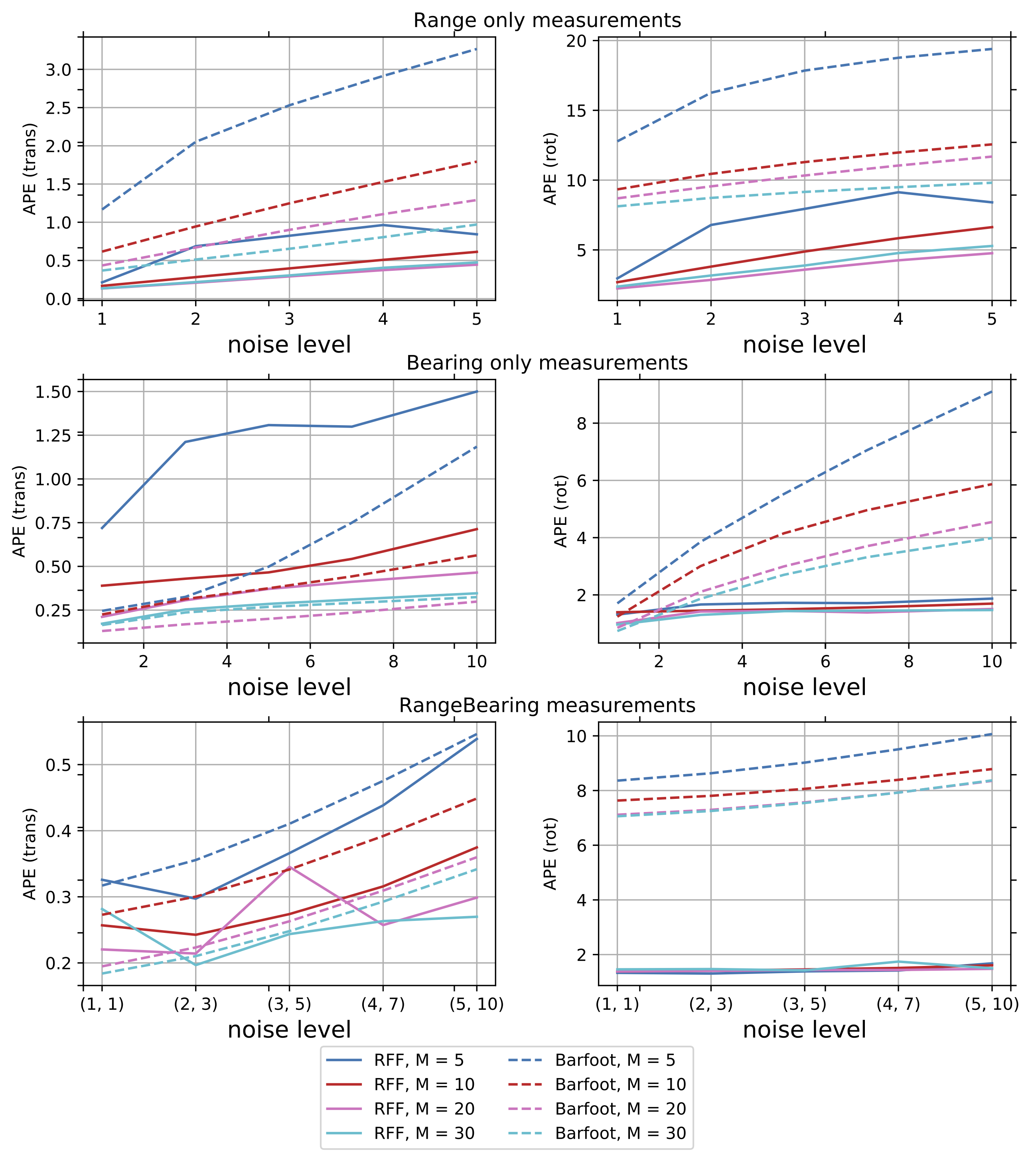
Figure 1: Average APE errors for synthetic trajectories at different noise levels and number of landmarks

TABLE I: Relative Errors for synthetic trajectories

		Pos.	Rot.	Landmarks
RangeBearing	RFF	0.022	0.154	6e-4
	LTV SDE	0.025	5.602	0.110
Range	RFF	0.016	0.320	1e-6
	LTV SDE	0.025	5.580	0.003
Bearing	RFF	0.035	0.152	8e-6
	LTV SDE	0.025	1.200	0.016

IV-2 Autonomous Lawn-Mower

In this experiment we evaluate our approach on a Plaza data set collected from an autonomous lawn-mower [31]. The data set contains range measurements recorded using time-of-flight and odometry measurements. Odometry measurements come more frequently than range measurements. The ground truth data was collected from GPS measurements and according to [31] its accuracy is $2$cm. The resulting trajectory is given in Figure 2. In this experiment we did batch updates with batch size $5$, i.e. we updated the trajectory after each new $5$ measurements. The motion model based prior was used as we have odometry measurements. We can see slight oscillations of the estimated trajectory. They can be explained by the nature of the Fourier features. However, the errors are comparable, see Table II. The estimated trajectories are depicted in Figure 2.

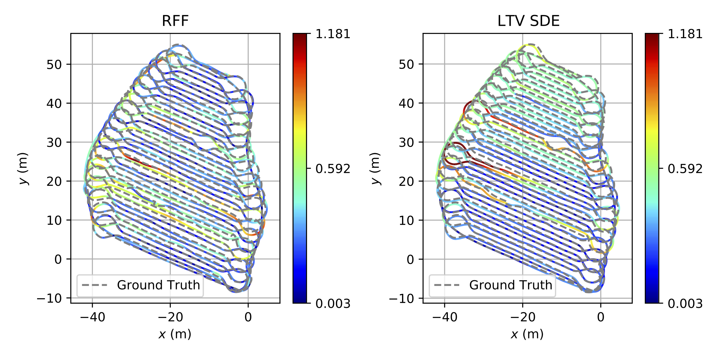
Figure 2: Distribution of APE errors along the trajecotry for Autonomous Lawn-Mower benchmark

IV-A KITTI-projected dataset

To evaluate our approach, we proceed with the famous dataset KITTI odometry[32]. We used the dataset part with a sequence of stereo images taken while moving along a specific trajectory. The dataset also contains ground truth trajectory and camera information. To apply our approach, we extracted bearing observations by using visual SLAM from ORB-SLAM2 [33]. From each stereo image we find keypoints with their coordinates in the local frame [34] which we use to calculate bearing observations. The keypoints in this case play the role of landmarks. The pipeline to project KITTI into a 2D dataset is following:

• Input: KITTI-odometry datasett(e.g. sequence 08);

• Run ORB-SLAM2 to get observations (keypoints, timestamps);

• Correct camera pose and keypoints by a transformation term that aligns with the vertical axis to make them independent of their original camera pose

  $$R_{t}\cdot R_{correction}=\mathrm{Exp}([0,0,\alpha]^{\top});$$ (11)

• Calculate weights for each observations based on how much time this point was observed/visited;

• Filter observations;

• Do orthonormal projection for each observation;

• Calculate bearing.

The number of landmarks (keypoints) is $80771$. With such a big number of landmarks, the experiments are very slow, so we reduced the number of landmarks to $3975$. We selected the landmarks randomly with probabilities proportional to their weights, but for each keyframe we left not less than $10$ landmarks. Also, to speed up the calculations we split the trajectory into $10$ consecutive slices, do estimation on each slice independently and then average the estimation errors.

The extracted data we then use in our approach to estimate the trajectory. To check our assumption that kernels with dense precision matrices should work better in case of noisy observations, we also generated a noisy version of the KITTI-projected dataset. To do so, we added Gaussian noise with standard deviation $\sigma$.

The results are given in Table II. We can see that without additional noise the results are comparable (with RFF based approach being slightly better). When we increase the amount of noise, absolute errors of our approach grow much slower compared to LTV SDE errors.

TABLE II: Real-world benchmark errors.

Autonomous Lawn-Mower
	APE (trans)	APE (rot)	RPE (trans)	RPE (rot)
LTV SDE	$0.48$	$1.44$	$0.021$	$0.10$
RFF	$0.42$	$2.25$	$0.026$	$0.54$
KITTI-projected
LTV SDE	$5.130$	$1.059$	$0.068$	$0.113$
RFF	$5.070$	$0.489$	$0.040$	$0.048$
KITTI-projected + noise, $\sigma=1^{\circ}$
LTV SDE	$5.126$	$1.086$	$0.068$	$0.133$
RFF	$5.070$	$0.544$	$0.0454$	$0.052$
KITTI-projected + noise, $\sigma=3^{\circ}$
LTV SDE	$5.491$	$3.136$	$0.139$	$0.259$
RFF	$5.075$	$1.027$	$0.073$	$0.115$
KITTI-projected + noise, $\sigma=5^{\circ}$
LTV SDE	$12.915$	$5.114$	$0.242$	$0.358$
RFF	$5.077$	$1.304$	$0.084$	$0.119$

V CONCLUSION

In this paper, we show how to apply GP for time-continuous SLAM with a less restricted class of kernel functions. We accomplish it by using RFF approximation of the kernel. The proposed approach has linear complexity in number of observations $N$, which is much faster compared to the traditional GP model. The method provides a lot of flexibility for tuning various aspects of the state estimate (smoothness, periodicity, etc.) by choosing an appropriate kernel function. However, such flexibility requires more careful tuning of the prior parameters (mainly, we need good prior mean for the trajectory and careful balance between measurements covariance, weights and landmarks prior covariances). We demonstrated the potential of the approach on synthetic and real world datasets. The experiments justify our assumption that in the case of noisy observations having dense inverse covariance matrix helps to improve the accuracy compared to sparse matrices.

References

- [1] T. Bailey and H. Durrant-Whyte, “Simultaneous localization and mapping (slam): Part ii,” IEEE robotics & automation magazine, vol. 13, no. 3, pp. 108–117, 2006.
- [2] H. Durrant-Whyte and T. Bailey, “Simultaneous localization and mapping: part i,” IEEE robotics & automation magazine, vol. 13, no. 2, pp. 99–110, 2006.
- [3] S. Thrun, W. Burgard, and D. Fox, Probabilistic robotics. MIT press, 2005.
- [4] F. Dellaert and M. Kaess, “Square root sam: Simultaneous localization and mapping via square root information smoothing,” The International Journal of Robotics Research, vol. 25, no. 12, pp. 1181–1203, 2006.
- [5] X. Wang, R. Marcotte, G. Ferrer, and E. Olson, “Apriisam: real-time smoothing and mapping,” in 2018 IEEE International Conference on Robotics and Automation (ICRA). IEEE, 2018, pp. 2486–2493.
- [6] A. Cunningham, V. Indelman, and F. Dellaert, “Ddf-sam 2.0: Consistent distributed smoothing and mapping,” in 2013 IEEE international conference on robotics and automation. IEEE, 2013, pp. 5220–5227.
- [7] E. Strömberg, “Smoothing and mapping of an unmanned aerial vehicle using ultra-wideband sensors,” 2017.
- [8] J. Dong and Z. Lv, “minisam: A flexible factor graph non-linear least squares optimization framework,” arXiv preprint arXiv:1909.00903, 2019.
- [9] M. Kaess, A. Ranganathan, and F. Dellaert, “isam: Incremental smoothing and mapping,” IEEE Transactions on Robotics, vol. 24, no. 6, pp. 1365–1378, 2008.
- [10] ——, “isam: Fast incremental smoothing and mapping with efficient data association,” in Proceedings 2007 IEEE International Conference on Robotics and Automation. IEEE, 2007, pp. 1670–1677.
- [11] M. Kaess, V. Ila, R. Roberts, and F. Dellaert, “The bayes tree: An algorithmic foundation for probabilistic robot mapping,” in Algorithmic Foundations of Robotics IX. Springer, 2010, pp. 157–173.
- [12] T. D. Barfoot, C. H. Tong, and S. Särkkä, “Batch continuous-time trajectory estimation as exactly sparse gaussian process regression.” in Robotics: Science and Systems, vol. 10. Citeseer, 2014.
- [13] T. D. Barfoot, State Estimation for Robotics. Cambridge University Press, 2017.
- [14] P. Furgale, T. D. Barfoot, and G. Sibley, “Continuous-time batch estimation using temporal basis functions,” in 2012 IEEE International Conference on Robotics and Automation. IEEE, 2012, pp. 2088–2095.
- [15] C. Bibby and I. Reid, “A hybrid slam representation for dynamic marine environments,” in 2010 IEEE International Conference on Robotics and Automation. IEEE, 2010, pp. 257–264.
- [16] M. Fleps, E. Mair, O. Ruepp, M. Suppa, and D. Burschka, “Optimization based imu camera calibration,” in 2011 IEEE/RSJ International Conference on Intelligent Robots and Systems. IEEE, 2011, pp. 3297–3304.
- [17] D. Droeschel and S. Behnke, “Efficient continuous-time slam for 3d lidar-based online mapping,” in 2018 IEEE International Conference on Robotics and Automation (ICRA). IEEE, 2018, pp. 1–9.
- [18] C. H. Tong, P. Furgale, and T. D. Barfoot, “Gaussian process gauss-newton for non-parametric simultaneous localization and mapping,” The International Journal of Robotics Research, vol. 32, no. 5, pp. 507–525, 2013.
- [19] X. Yan, V. Indelman, and B. Boots, “Incremental sparse gp regression for continuous-time trajectory estimation and mapping,” Robotics and Autonomous Systems, vol. 87, pp. 120–132, 2017.
- [20] T. D. Barfoot, C. H. Tong, and S. Särkkä, “Batch continuous-time trajectory estimation as exactly sparse gaussian process regression.” in Robotics: Science and Systems, vol. 10. Citeseer, 2014.
- [21] A. Rudi, L. Carratino, and L. Rosasco, “Falkon: An optimal large scale kernel method,” in Advances in Neural Information Processing Systems, 2017, pp. 3888–3898.
- [22] K. Wang, G. Pleiss, J. Gardner, S. Tyree, K. Q. Weinberger, and A. G. Wilson, “Exact gaussian processes on a million data points,” in Advances in Neural Information Processing Systems, 2019, pp. 14 622–14 632.
- [23] M. Munkhoeva, Y. Kapushev, E. Burnaev, and I. Oseledets, “Quadrature-based features for kernel approximation,” in Advances in Neural Information Processing Systems, 2018, pp. 9147–9156.
- [24] J. Quiñonero-Candela and C. E. Rasmussen, “A unifying view of sparse approximate gaussian process regression,” Journal of Machine Learning Research, vol. 6, no. Dec, pp. 1939–1959, 2005.
- [25] A. Rahimi and B. Recht, “Random features for large-scale kernel machines,” in Advances in neural information processing systems, 2008, pp. 1177–1184.
- [26] C. E. Rasmussen, “Gaussian processes in machine learning,” in Advanced lectures on machine learning. Springer, 2004, pp. 63–71.
- [27] E. Burnaev, M. Panov, and A. Zaytsev, “Regression on the basis of nonstationary gaussian processes with bayesian regularization,” Journal of communications technology and electronics, vol. 61, no. 6, pp. 661–671, 2016.
- [28] W. Rudin, Fourier analysis on groups. Courier Dover Publications, 2017.
- [29] K. M. Choromanski, M. Rowland, and A. Weller, “The unreasonable effectiveness of structured random orthogonal embeddings,” in Advances in Neural Information Processing Systems, 2017, pp. 219–228.
- [30] C. De Boor, “A practical guide to splines, revised edition,” 2001.
- [31] J. A. Djugash, “Geolocation with range: Robustness, efficiency and scalability,” 2010.
- [32] A. Geiger, P. Lenz, C. Stiller, and R. Urtasun, “Vision meets robotics: The kitti dataset,” The International Journal of Robotics Research, vol. 32, no. 11, pp. 1231–1237, 2013.
- [33] R. Mur-Artal and J. D. Tardós, “Orb-slam2: An open-source slam system for monocular, stereo, and rgb-d cameras,” IEEE Transactions on Robotics, vol. 33, no. 5, pp. 1255–1262, 2017.
- [34] R. Hartley and A. Zisserman, Multiple view geometry in computer vision. Cambridge university press, 2003.