A general modelling framework for open wildlife populations based on the Polya Tree prior–LABEL:lastpage
A general modelling framework for open wildlife populations based on the Polya Tree prior
Abstract
Wildlife monitoring for open populations can be performed using a number of different survey methods. Each survey method gives rise to a type of data and, in the last five decades, a large number of associated statistical models have been developed for analysing these data. Although these models have been parameterised and fitted using different approaches, they have all been designed to model the pattern with which individuals enter and exit the population and to estimate the population size. However, existing approaches rely on a predefined model structure and complexity, either by assuming that parameters are specific to sampling occasions, or by employing parametric curves. Instead, we propose a novel Bayesian nonparametric framework for modelling entry and exit patterns based on the Polya Tree (PT) prior for densities. Our Bayesian non-parametric approach avoids overfitting when inferring entry and exit patterns while simultaneously allowing more flexibility than is possible using parametric curves. We apply our new framework to capture-recapture, count and ring-recovery data and we introduce the replicated PT prior for defining classes of models for these data. Additionally, we define the Hierarchical Logistic PT prior for jointly modelling related data and we consider the Optional PT prior for modelling long time series of data. We demonstrate our new approach using five different case studies on birds, amphibians and insects.
keywords:
Bayesian nonparametrics, capture-recapture, count data, Polya tree, ring-recovery, statistical ecology.1 Introduction
In recent years, there has been an increased interest in monitoring wildlife populations due to the ongoing effects of climate change and habitat destruction. However, monitoring wildlife populations is challenging because it is difficult to observe all animals present in the wild. Therefore, statistical models need to be employed to infer population sizes (Royle, 2004), migration (Pledger et al., 2009), phenological (Dennis et al., 2017) or survival patterns (McCrea et al., 2013) from ecological data at one or more sites.
Although these models are developed for data collected using different sampling protocols, they all focus on the estimation of the entry, exit and length of stay (LOS) patterns of populations, where entry can correspond to arrival/birth, exit to departure/death and LOS to retention/survival at the site. These existing methods either assume that parameters related to entry and exit patterns are completely unconstrained, requiring two parameters to be estimated for each sampling occasion, one for entry and one for exit (Pledger et al., 2009; Lyons et al., 2016), or use parametric curves to constrain entry (Matechou et al., 2014) and exit patterns (McCrea et al., 2013; Jimenez-Muñoz et al., 2019). In recent years, Bayesian nonparametric (BNP) methods have been used in ecology to flexibly model entry and exit distributions without making parametric assumptions. In particular, models have been built using the Dirichlet Process (DP) mixture prior (Lo, 1984), which is a model for continuous distributions relying on a mixture model, see for example Ford et al. (2015); Matechou and Caron (2017); Diana et al. (2020), or using the Polya Tree (PT) prior (Ferguson, 1974), such as in Diana et al. (2018).
In ecological surveys, data are typically collected at discrete times, referred to as sampling occasions. Every pair of consecutive sampling occasions defines an interval, during which individuals may enter or exit the study area. No data are available for the periods between sampling occasions. This suggests that when inferring entry and exit patterns we need to model the grid defined by the sampling occasions in the bivariate space of entry and exit. In this paper, we develop a general BNP framework for modelling this grid, based on the PT prior, which was also considered by Diana et al. (2018). The PT prior is a nonparametric prior for densities that is constructed by defining an infinite sequence of nested partitions of the sample space and recursively assigning the masses of the elements of each partition. In our case, we only need to define the PT for a finite sequence of partitions up to the level of the grid, which defines a prior distribution for the probabilities of an individual to fall in each cell of the grid. Our new modelling framework allows us to build models directly on the distribution of entry, exit and LOS, with minimal parametric assumptions on the shape of these distributions. We note that, in contrast to existing BNP approaches based on DP mixtures that build continuous models, our approach allows us to make inference directly from the latent number of individuals in each cell of the grid, with computational complexity only depending on the number of sampling occasions and not the number of individuals in the population, leading to substantial computational advantages.
Another advantage of the PT framework is that it can be extended in various directions. To extend the model to data collected at different sites or years, we define the replicate PT (RPT), which shares random variables (r.v.s) across different PTs, allowing us to impose constraints on model parameters, and the Hierarchical Logistic PT (HLPT), which allows us to model r.v.s across different distributions in a hierarchical fashion, implying exchangeability across the different units.
We apply our approach to four different case studies. The first considers the estimation of entry and exit densities by a joint model of capture-recapture (CR) and count data (CD) collected on the same population. The second considers the estimation of age-specific survival, i.e. LOS, using ring-recovery (RR) data, where only some of the individuals are of known age, and demonstrates the advantage of the PT in modelling survival from sparse data, without resorting to the use of parametric curves. The third application involves estimating entry and exit densities at different sites using the HLPT. Finally, the fourth scenario considers a long time-series of CD. For long time-series, choosing a partition at the frequency that the data are sampled leads to a large number of parameters. To overcome this problem, we use the Optional Polya Tree (OPT) of Wong and Ma (2010), which is an extension of the PT and allows us to infer the partition structure.
The paper is structured in the following way. In Section 2.1 we provide an overview of the sampling schemes considered as case studies in the paper. In Section 2.2 we describe the main features of the PT prior. In Section 3 we present and motivate the univariate partitions of the PT used in the paper and demonstrate the concept using CR data. The RPT prior is defined in Section 4. In Section 5.1 we define the bivariate partitions of the PT and define the joint model for CR data and CD and the model for RR data. The HLPT is defined in Section 6.1 and the use of the OPT is described in Section 6.2, with both sections presenting an application to CD collected across several species and years, respectively. Section 7 concludes the paper and introduces some potential future directions.
2 Background
2.1 Sampling schemes of population surveys
In this paper, we consider models for data resulting from three types of ecological sampling schemes: CR, CD and RR. In all three cases, we assume sampling is performed on sampling occasions at times .
In the case of CR data, on each sampling occasion, a sample of the individuals is caught, and newly caught individuals are uniquely marked. If is the total number of captured individuals, the captures can be summarised in a matrix, , where is if the -th individual was captured on sampling occasion and otherwise. Each row of the matrix is called a capture history. We define instead as presence history the vector with entries equal to on sampling occasions when the individual was available for capture and otherwise. A commonly employed approach for modelling CR data is the Cormack-Jolly-Seber (CJS) model (Cormack, 1964; Jolly, 1965; Seber, 1965). The CJS model is built conditional on the time of first capture of each individual. After the first capture, alive individuals of age at time are assumed to remain alive at the site until the following sampling occasion at time with probability and, conditionally on being present at the site, they can be recaptured (or resighted) with probability . Since the CJS model conditions on first capture, it does not allow the estimation of the population size but only of and . In the following, we will always use the indexes , and to indicate the times of first possible capture, first capture and last possible capture, respectively. We express the CJS model in a PT framework in Section 3.1.
CD are collected by visiting the site and simply detecting a number of individuals, without attempting to individually identify them. The data can be summarised in a vector , where denotes the number of individuals detected on sampling occasion .
Finally, according to the RR protocol, individuals are captured and marked each year and, after being marked, they can be recovered soon after they die with probability . The data are usually summarised in an upper-triangular matrix, , where cell denotes the number of individuals marked in year and recovered dead in year , and in a vector where denotes the total number of individuals marked in year .
2.2 The Polya Tree prior
The Polya tree (PT) prior (Ferguson, 1974) is a nonparametric prior for probability distributions. It has two parameter sets: the first is a sequence of nested partitions of the sample space , while the second parameter, , is a sequence of positive numbers associated with each set of each partition.
The partition at the first level, , is obtained by splitting the sample space in sets . Subsequently, to build the partition at the second level, , each set is split into sets , next each set is split into sets and so on. We note that for dyadic splits, the Dirichlet distributions are replaced by Beta distributions.
By defining as a generic sequence of positive integers (such that ) and as the correspondent set of the partition, the random mass associated to by the PT is given by , where and for . For example, in the case where splits are triadic, where Dirichlet and Dirichlet. The s can be interpreted as the conditional probabilities of falling in a particular set in the next level of the tree, that is, given , where , .
The PT is a conjugate prior for a distribution if we have observations , since the posterior distribution is a PT with parameters and , where and is the number of observations falling into set . The PT can be centered on any distribution in the sense that, for every set of the partition, .
3 Univariate PT models
The partition of the PT can be chosen according to the specific application. To define a prior for the distribution of a time-to-event on the real line, Lavine (1994) (L94) proposed the following partition. Assume we have sampling times and we only observe the interval where each time-to-event happens, that is, we observe whether , and so on. L94 proposed to define such that , , with further split into , and so on. A representation is shown in Fig. 1. Following the notation of Section 2.2, this structure is obtained when and .
Samples from a PT with the partition defined above have decreasing variance starting from the earlier sampling times. This follows easily from the following proposition, proven for simplicity for Beta r.v.s with mean .
Proposition \thetheorem
Given and , if then .
The previous proposition shows that if the r.v.s , assigning the masses to the sets , , have parameters whose sum is not decreasing, the variance of , , , is decreasing. Conversely, we can assume that the variance is decreasing starting from the last sampling times by reversing the order of the split and splitting the partition using first , then and so on. We term the two partitions defined above as the forward LOS partition (FLP) and backward LOS partition (BLP), respectively. The idea of L94 is useful when modelling ecological data since, as mentioned above, sampling is typically performed only at discrete times, . An application of this partition is presented in Section 3.1.
In some cases, it is useful to build the partition in a single step by splitting using all the sampling times simultaneously. That is, we split in , where and , , and the masses are assigned according to a Dirichlet distribution. This choice implies negative correlation between probabilities of any two disjoint sets. This partition is termed the uniform partition (UP).
3.1 Example: Cormack-Jolly-Seber
In this section we demonstrate how the CJS model, briefly described in Section 2.1, can be expressed in a PT framework. Following the original CJS model formulation, we define the model for the data conditioning on the time of first capture.
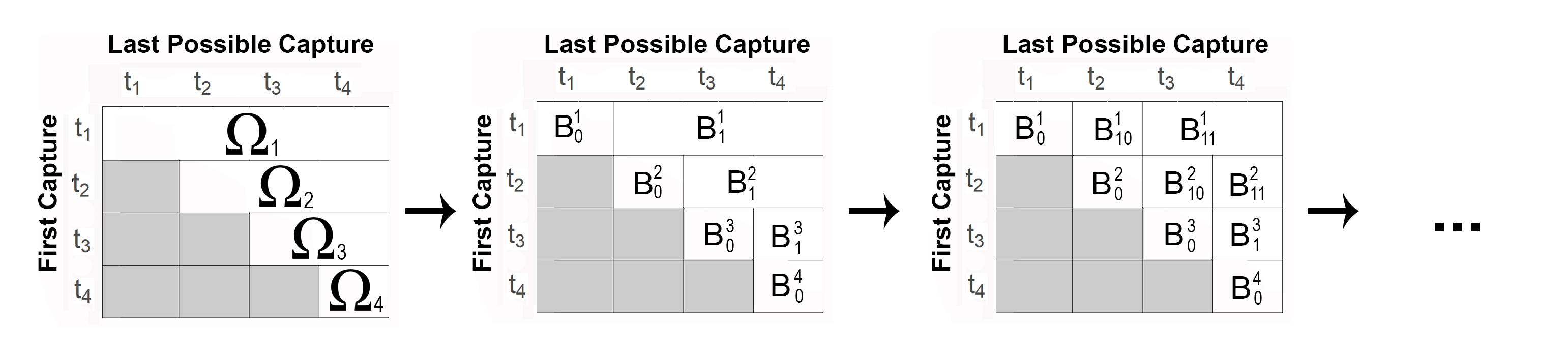
We first arrange all the marked individuals in a set of vectors , where indicates the number of individuals with first capture at time and remaining at the site for sampling occasions or, equivalently, with last possible capture at time . Next, we assume a distribution on the time of last possible capture for the individuals belonging to vector or, equivalently, for the individuals with first capture at time . The sample space for is , as exit time is left truncated by the time of first capture. We assume a PT prior for each , with partition taken to be the FLP. According to the FLP, the sample space is split into and , next is further split into and and so on. The last level of the partition corresponds to the grid defined by the capture times, , and thus it uniquely determines the probabilities of each cell. A visual representation of the sets of the sample space is shown in Fig. 2. The partitions have different depths as for the individuals with first capture at time , the partition is built only for levels.
For illustration purposes, we assume that individuals are of age when first caught at time but will later show how to relax this assumption. We define to be the probability of an individual aged when first caught at time exiting before time conditional on being present and of age at the site at time . The can also be seen as the ratio of masses (where ) in the PT.
As mentioned in Section 2.1, in the standard CJS model, corresponds to the probability that an individual present and aged at time remains until time . As individuals first caught at time are of age at time , according to our model .
The advantage of using a PT prior is that different assumptions regarding the model for parameter can be considered by sharing the r.v.s across the different PTs. We list below a number of assumptions that can be made and demonstrate the concept by writing the probability of capture history , , according to each assumption.
-
•
Constant case: . .
-
•
Age-dependent case: , that is equivalent to assuming that . .
-
•
Time-dependent case: . This is equivalent to assuming that the distribution of is the same as the distribution of . .
-
•
Unconstrained case: The most general case is obtained by assuming that all the are different. Although this model is never fitted in practice because it is overparametrised, we can still write as .
These assumptions are depicted in Fig. 3. The likelihood of the data and the MCMC algorithm used to sample from the posterior distribution are respectively in Section and of the supplementary material.
4 Replicate PT
In the CJS model defined in the previous section, different models are obtained by assuming that parts of different trees are “replicated” across different branches. The same idea will also be used in the next sections, and hence we provide a formal definition of the RPT. The definition we provide is for a single tree but it is easy to extend to the case of multiple trees.
Let be a rule to generate a sequence of partitions from an initial seed set. For example, in the CJS example the rule corresponds to FLP and the seed sets are . If is a distribution having a PT prior with partition , we say that has a Replicate PT (RPT) structure across two sets and of the partition if the following constraints hold:
-
•
The partitions of the trees starting from and are generated according to the same rule , although the two partitions could be stopped after a different number of steps;
-
•
For all , .
The first condition states that the partitions of the trees starting from and are the same for a number of steps, while the second states that the r.v.s in the two trees are the same. The assumption that the r.v.s are shared across different parts of the tree does not change the conjugate scheme described in Section 2.2. The definition is easily extended to the case where more than two parts of a tree are shared.
Some of the assumptions of the CJS model, depicted in Fig. 3, can be expressed in terms of the RPT just defined. The age-dependent case is obtained assuming that the trees have a replicate structure across the sets , while the time-dependent case is obtained assuming a replicate structure across the pairs of trees with seed sets: and , and , and and so on.
For ease of exposition, in all the case studies shown later, we only consider the most commonly employed constraint in each case. However, similarly to the CJS case described above, different RPT structures can be employed in order to assume different constraints if required.
5 Bivariate PT models
5.1 Bivariate partitions
In this section, we extend the model for CR data conditional on the time of first capture of Section 3.1 to two scenarios: CR without conditioning on first capture and RR. To highlight the connection with D18, we briefly describe their model here. D18 define a model for count data by introducing a matrix of the individuals with first possible detection at time and last possible detection at time . Therefore, inferring matrix , which also includes information on the latent entry intervals, gives rise to an estimate of the entry and exit pattern and the size of the population.
In the CR and RR extensions, we do not condition on first capture as in the CJS but we model the entry intervals of the individuals, and thus instead of working with a set of vectors we will introduce a set of matrices , similarly to D18. We note that, as opposed to D18, in the case of uniquely identifiable individuals, as in CR and RR data, the time of first capture is also needed to obtain an analytical expression for the likelihood function. However, the downside of adding another dimension is that it increases the number of parameters of the model. Hence, we share information between individuals with different times of first capture by using the RPT structure, in a similar fashion as this was performed for the CJS model.
The RR and CR models are built by using the same set of matrices to summarise the entry and exit patterns, but we demonstrate how different prior distributions can be elicited depending on whether prior knowledge is available on entry and exit (CR) or LOS (RR).
In order to define the aforementioned models, we need to define partitions for distributions on , as we consider joint distributions on entry and exit or on entry and LOS. Partitions for distributions on can be defined by using the schemes defined in Section 3 separately for each dimension. We note that do not consider partitions built by considering splits in more than one dimension at a time, such as in Paddock et al. (2003), for two reasons. First, building univariate partitions sequentially for each dimension makes it easier to center the PT on standard parametric models. For example, if the distribution of interest is the bivariate entry and exit distribution, building a sequential model by splitting first according to entry and then according to exit assumes a centering model where exit is independent on entry. Secondly, interpretation from the model by considering joint splits becomes more difficult. In fact, inference on the conditional distribution of one dimension given the other is not straightforward to obtain anymore in this case.
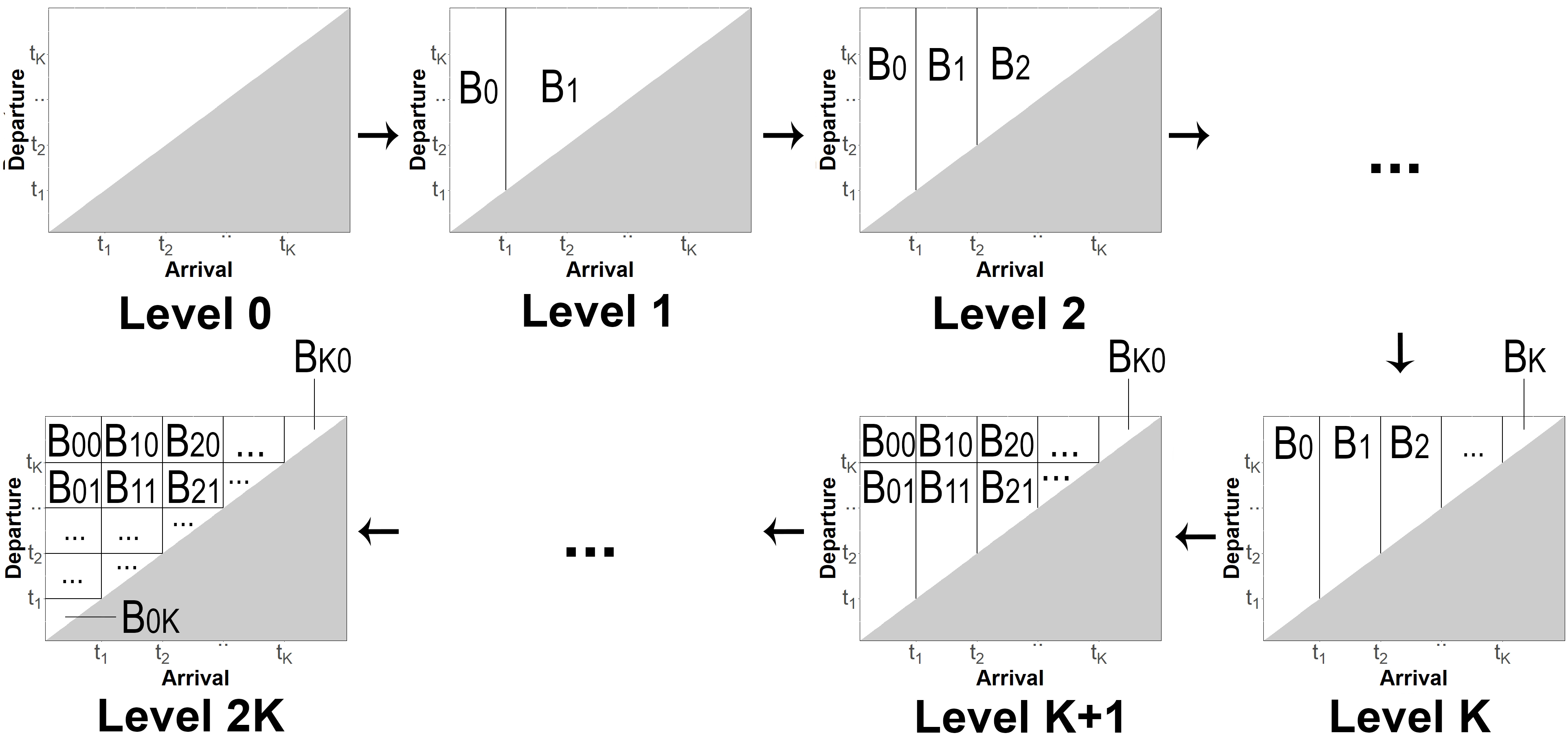
A useful bivariate partition can be constructed by applying first FLP in one dimension and next BLP in the other. We denote this partition as entry and exit bivariate partition (EEBP), and the scheme is depicted in Fig. 4. A formal definition of the partition is presented in Section of the supplementary material.
This partition is useful when the entry and exit distribution is of interest, as the marginal distribution of entry is expected to have more variance in the left tail, while for the marginal exit distribution more variance is assumed in the right tail. This partition is used in D18, who built a model for CD based on a PT. The model is further extended to CR data in Section 5.2.
When no prior information is available on the variance of the entry or exit distributions, the forward/backward splits can be replaced by the uniform split (UP), described in Section 3, shown in Fig. of the supplementary material and used in Section 6.2.
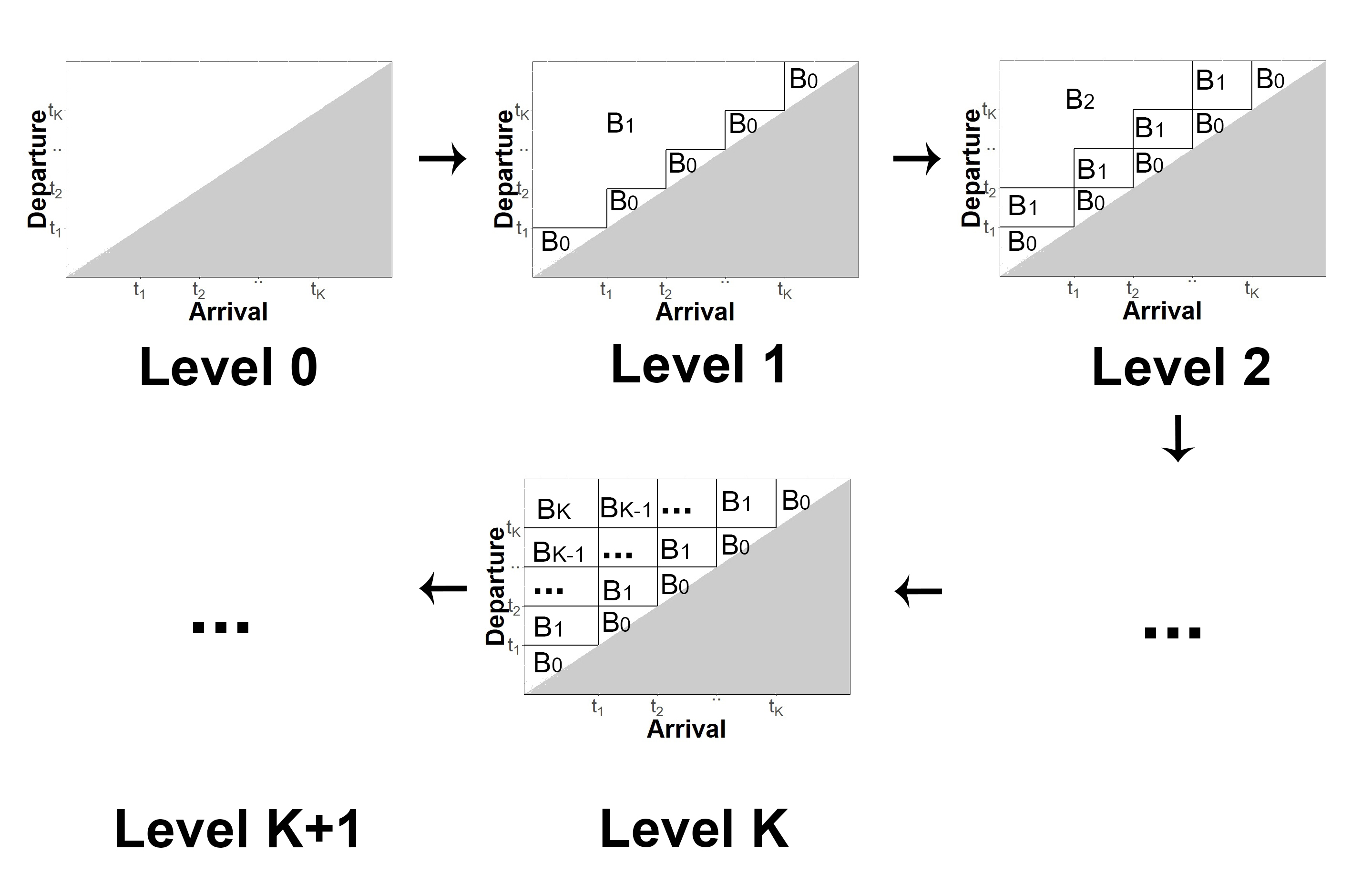
The two previous partitions allow us to elicit prior information on the entry and exit distribution. However, as mentioned above, in some applications, prior information is available on the LOS distribution instead. For eliciting a prior on the LOS distribution, we define a bivariate partition based on the idea of L94 but split the sample space w.r.t. the LOS and then w.r.t the entry intervals, as shown in Fig. 5. The definition is given in Section of the supplementary material. This partition is termed bivariate LOS partition (BivLP) and an application is presented in Section 5.3.
5.2 Joint analysis of capture-recapture and count-data
Recent work (Barker et al., 2018) casted doubt on whether CD alone can be used to provide reliable estimates of population size and suggested that analysis of CD should be augmented by other types of data, such as CR. Therefore, in this section, we demonstrate how to extend D18 to perform a joint analysis of CR and CD using an RPT. As introduced in the previous section, we define the set of matrices , where denotes the number of individuals with first possible capture at time , first capture at time and last possible capture at time (clearly, for ). For , we define as the matrix containing the individuals never captured, but possibly detected and hence contributing to the CD.
For each matrix , we define a distribution on the probabilities of an individual belonging to each cell of the matrix , and we assume a PT prior for each using the EEBP partition of Section 5.1. We make the assumption that the distribution of entry and exit intervals is the same for each matrix . If is the sample space for the individuals with first capture at time , this is achieved by assuming a RPT prior across the sets , as in Section 3.1. Moreover, we also assume that the exit distribution is independent of the entry interval, which is achieved by assuming, for each slice , a RPT structure across the sets , , , (see level of Fig. 4 for a visual representation of the sets).
We note that each matrix is defined on a different sample space, as is defined only for , because individuals in the -th slice have to enter before the -th sampling occasion and exit after. A representation of one slice is shown in Fig. of the supplementary material.
We define the sum of the elements of matrix as . However, while is known for (as it is equal to the number of individuals with first capture at time ), is unknown as it corresponds to the number of individuals never captured. Given the number of individuals , the number of individuals in each cell of the matrix is distributed as a multinomial with sample size and vector of probabilities . The total number of individuals is then equal to , where is the number of caught individuals. We also define as the number of individuals available for capture/detection at time , conditional on the latent matrices . Assuming a prior distribution for , the model can be summarised as
where and are the probability of detecting and capturing an individual, respectively. The probability of the capture histories of the individuals with first capture at time , conditional on the matrix , is presented in Section of the supplementary material.
5.2.1 Case study
We apply our model to CD and CR data collected on a population of Italian spoonbills (Platalea leucorodia) collected in the southern Po delta, in North-East Italy. Birds are captured as chicks in previous years and are uniquely marked. The CR dataset is collected by resighting adult birds through photographs obtained using camera traps and by visiting their nests on eight separate sampling occasions. No attempt is made to mark new adult individuals and instead only previously marked individuals can be resighted. In addition, unmarked birds are detected on each sampling occasion. In this case, there are fewer than resighted individuals, so we choose to make inference by modelling individual entry and exit intervals for all the marked individuals resighted. The full details of the model are given in Section the supplementary material.
The posterior means of the entry and exit cumulative distribution functions (CDFs) are shown in Fig. (a) of the supplementary material. The CDF of the departure does not reach within the study period since some birds remain at the site using the colony as a roost. Similarly, the CDF of the arrival intervals is at around 0.4 at the start of the study, suggesting that a large proportion of birds are present at the site when sampling starts, with over 80% of birds estimated to have arrived by the second sampling occasion toward the end of April. The posterior distributions of the two population sizes and resighting probabilities are shown in Fig. (b) of the supplementary material. The camera trap resight probability, , is slightly lower than the resight probability through nest visits, , since cameras are pointed toward the nest, where it is unlikely to see floaters and prospectors. The difference between the population sizes of marked and unmarked birds is due to the fact that not all the chicks are marked each year, and out of those marked, only a small proportion return to breed as adults. In fact, local recruitment rate is thought to be around , while the proportion of immigrants on total number of recruits is ranges from to (Tenan et al., 2017).
5.3 Ring-Recovery
In this section, we show how to build a model for RR data using a RPT prior. Similarly to what was mentioned in Section 5.1, in order to jointly model entry and exit patterns we work with a set of matrices , where in this case represent the number of individuals marked on sampling occasion that were present in the population for sampling occasions before being marked and remained for sampling occasions after being marked. We assume that individuals marked at time could have entered the population for up to sampling occasions before they were marked and could have stayed for up to sampling occasions after being marked, and thus we assume the dimension of each matrix is .
For each matrix , we assume a PT prior for the probabilities for an individual to belong to each cell , with partition taken to be the BivLP partition built in Section 5.1. A visual representation of the partition for a matrix is presented in Fig. of the supplementary material.
Similarly to Section 3.1, we make the assumption that the survival probability is age-dependent, that is, the probability of an individual surviving until the next sampling occasion depends only on the age of the individual and not on the sampling occasion. If we define to be the sample space for the individuals marked at time , this assumption can be achieved by assuming an RPT across . This forces the probabilities to be the same for each , that is . If we define as the probability of an individual of age that is present at time to remain until the following sampling occasion, assuming an RPT prior over the different slices is equivalent to assuming that .
The number of individuals marked at time that can be recovered at time can be obtained by the matrix as by summing over the different entry times. Hence, the number of individuals marked in year recovered dead in year , , is distributed as a . Assuming also a Beta prior for the recovery probability , the model can be summarised as
| (1) |
5.3.1 Case study
We apply our model to a dataset collected in Minnesota, USA. A total of female mallards were banded throughout the course of the study, which lasted 51 years. Marking occurs from July to September, while recoveries occur during the hunting season immediately following marking, from September to January. Newly caught individuals can be recognized as juveniles if their age is less than year at the time of capture and as adults otherwise. Therefore, individuals caught as juveniles that have been recovered are of known age at year of death. The entry and exit of the individuals correspond in this case to births and deaths, while the sampling occasions correspond to the markings and recoveries. The full details of the model are given in Section of the supplementary material.
The posterior mean of the survival probabilities is presented in Fig. of the supplementary material. The result agrees with the general pattern observed for bird populations, with survival being lower in very young and older ages. A similar pattern was observed by McCrea et al. (2013) when analysing RR data for mallards (Anas platyrhynchos) and by Jimenez-Muñoz et al. (2019) for blackbirds (Turdus merula), but we note here that we have not employed a parametric curve to enforce this pattern, and instead if has been completely driven by the data. As expected, uncertainty increases for older ages because of the sparseness of the data. The posterior mean of the recovery probability is equal to , (95% PCI: ) which is in line with findings of similar studies (McCrea et al., 2012).
6 The hierarchical Logistic PT
The RPT defined in Section 4 allows us to impose constraints across different distributions or conditional distributions by assuming the same r.v.s across different trees or across different branches of the same tree, which in the case of density estimation forces the different distributions to be the same. This assumption is however too restrictive in many real applications, as for example when jointly modelling data collected across different years or sites. In these cases, it may be more reasonable to employ a hierarchical approach, which enables us to borrow strength across the different datasets but without assuming that the distributions describing the different datasets are exactly the same.
In the context of data collected at different units, Christensen and Ma (2020) propose a Hierarchical PT by assuming a PT prior in each unit, where each PT is centered on a common baseline PT prior. However, because of the lack of conjugacy of a Beta prior with a Beta likelihood, the sampling scheme relies on quadrature techniques. To employ a hierarchical approach while still performing inference with a Gibbs sampler, we suggest an alternative approach based on the logistic PT (LPT) of Jara and Hanson (2011). The LPT is defined by replacing the Dirichlet distributions for the in the definition of the PT with multinomial logistic normal distributions.
If are the distribution in each unit and are the conditional distributions assigning the mass in each split in the -th unit, that is , we define the hierarchical model as
where are the parameters of a PT centered on a distribution and an additional hyperprior is assumed on . A set of PTs following this structure will be termed Hierarchical Logistic PT (HLPT). If , we have and hence the distributions for each group are the same, reducing to the case of the RPT.
The LPT is defined in terms of a logistic transform of normal distributions and hence a Gibbs sampler, based on the Polya-Gamma scheme (Polson et al., 2013), is available, details of which can be found in Section of the supplementary material.
6.1 A hierarchical model across different datasets
In this section we extend D18 by defining a model for related datasets using the HLPT. The data consist of different datasets which, for ease of exposition, we take to be CD, but the same rationale applies for any other sampling schemes described before.
We define to be the number of individuals detected at time in the -th dataset. We arrange all the individuals in matrices , where is the number of individuals in dataset having first and last possible detection at times and , respectively. For the -th dataset, individual entry and exit times are drawn from a Poisson process with intensity , where is the overall intensity and is the normalized density. In order to borrow information between different datasets, the normalized densities are assumed to follow a HLPT prior, where the partition is taken to be the EEBP of Section 5.1.
Assuming also that each individual in dataset can be detected with probability , the model can be summarised in the following hierarchical structure
where is the number of individuals available for sampling on occasion and dataset .
6.1.1 Case study
We consider a dataset of weekly detections of species of newts separated by sex, resulting in different sets of CD, collected at a local site at the University of Kent in . Newts are usually sampled weekly during their breeding period using aquatic traps. However, some visits might be missed on occasion because of weather conditions. All three species migrate to ponds in late winter-early spring for breeding, and leave the breeding site in late spring or summer to spend the rest of the year on land. The data are shown in Figure of the supplementary material.
The posterior estimates of the entry and exit distributions for the datasets, shown in Fig. of the supplementary material, suggest that great crested newts tend to arrive and depart later than smooth or palmate newts. Additionally, males arrive earlier, while females depart later, since they need to complete egg-laying. All species are found to have similar detection probabilities with overlapping credible intervals, with the exception of palmate newts that have a slightly lower detection probability, as shown in Fig. of the supplementary material.
6.2 Modelling long time-series of ecological data
The last scenario we consider is a long time series of CD collected daily. The challenge that arises in this case is that the sampling period is considerably longer than the period during which individuals of the species are present at the site. Therefore, building a partition by considering all intervals would increase the computational complexity without necessarily providing a better description of the data. A naive modelling approach is to merge sampling occasions in order to obtain a shorter time series. However, the decision of how to merge is arbitrary and the same merging may not be meaningful for the duration of the study period. Instead, we let the model infer which sampling occasions to merge using the Optional Polya Tree of Wong and Ma (2010).
As in the model of Section 6.1, we build a prior distribution on the number of individuals present on each sampling occasion by assuming a PT prior on the individual entry and exit intervals. The partition of the PT is built using the UP of Section 5.1, where the splits are performed according to some nested periods of time, which for example can be taken as the natural scales at which data are collected, such as months, weeks and days. Using the OPT allows us to stop partitioning further, and hence the choice of the UP will lead the partition to end in one of these periods of time.
We divide the overall study period in periods of time of equal length, , called -periods, and we assume that individuals enter and exit only in the same -period. Next, for each -period, , we define a distribution on the entry and exit intervals of the individuals. The -periods can be thought of as the periods of time in which the entry and exit patterns seasonally repeat, such as the years. Next, as mentioned above, we define a set of splitting rules according to which the sample space of , is first split into the sets , and next, each set at level , , is split into . The sets in are called -periods. Given , we define as the set obtained by taking first the -th -period, then the -th -period and so on. For example, the years can be taken as the -periods and the splitting rules can be built using first the months as -periods, weeks as -periods and so on.
Next, given two sequences of indexes and , we define as the number of individuals in the -period entering in and exiting in . We also define as and the number of individuals available for sampling and detected, respectively, in the interval in the -th -period. Even if an explicit formula is cumbersome to present, it is straightforward to obtain the latent individuals from the . Thanks to this construction, we have defined a prior on the probabilities of an individual to belong to cell .
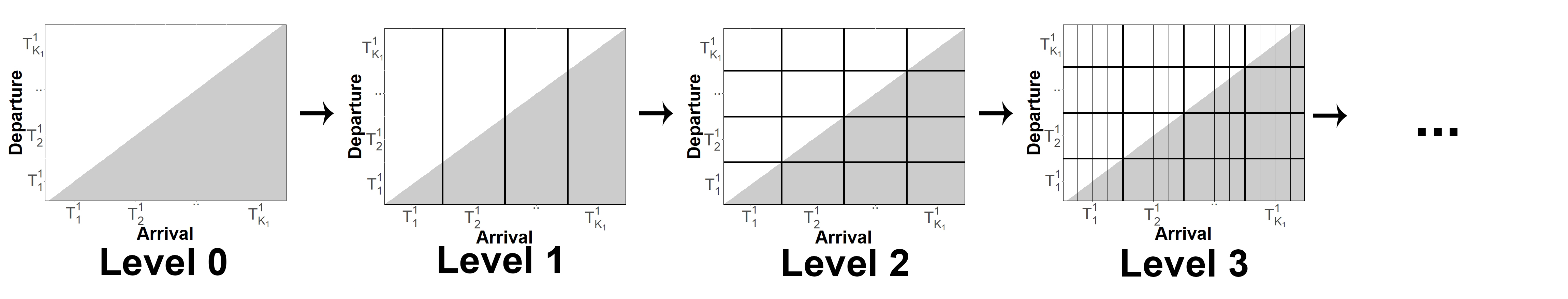
Having defined this set of splitting rules, we define the partition of sample space by first splitting in where , that is, the sample space is split using the dimension of entry according to the -periods. Next, each is split into , where , that is, each set is now split using the dimension of exit according to again the -periods. The next sets are split in an analogous way. A representation of this scheme is shown in Fig. 6. For the r.v.s assigning the masses in each level of the partition, we assume an HLPT structure across the years and, similarly to Section 5.2, we use an RPT structure to enforce that individuals arriving in different sets share the same departure distribution. Full details are given in Section of the supplementary material.
Assuming a Poisson prior distribution on the number of individuals in each -period, the model can be summarised in the following hierarchical structure
where is the probability of detecting an individual.
The downside of this model is that the partition is built for each period, even if no observations are available in some periods. Ideally, we would like to use a modelling approach where we keep partitioning the PT only in the periods of time where the entry and exit density has significant variation. To do so, we borrow ideas from the OPT of Wong and Ma (2010) and allow for different branches of the tree to not partition further.
Specifically, we assume that in each step, partitioning of the PT into the further level happens with probability . We then introduce a variable which is equal to if is not partitioned further and otherwise. The distribution in the set can be expressed recursively from its descendant sets as
where is the uniform distribution and are the descendant sets of . Hence, when no splitting is required we replace the PT distribution with a uniform distribution.
6.2.1 Case study
We consider a long series of daily CD of two indistinguishable species of moths, Canadian Melanolophia (Melanolophia canadaria) and Signate Melanolophia (Melanolophia signataria), collected across years (Pickering, 2015). The data are shown in Section of the supplementary material. Detection of the individuals is possible only during the flight period, which is known to happen only in a limited period of time inside the calendar year.
The posterior means of the entry and exit CDFs are shown in Fig. of the supplementary material. The exit pattern is practically identical between the different years, with the c.d.f suggesting a smooth exit pattern with a few bigger exit waves around weeks , and (start of September). On the other hand, entry patterns present more variation across years. The species are known to have two broods (Covell Jr, 1984), which is evident by the two big entry waves each year around weeks 20 and 24 (mid May) for all years apart from 2013, when the first brood emerged much earlier. This is likely due to the unusual warm temperature at the start of , as Table in the supplementary material suggests.
7 Conclusion
We introduced a framework for defining models for ecological data on open populations based on the PT prior. The advantage of this framework is that a wide variety of assumptions can be made on the model structure by changing the tree structure, as a result of the flexibility of the PT. We have applied our framework to different types of commonly collected ecological data, such as CR, CD and RR. We have also introduced the RPT, which allows us to place constraints on the model parameters, and the HLPT, which allows us to impose a hierarchical structure and share information when modelling different datasets. We have also presented a way to infer the partition of a PT using the OPT of Wong and Ma (2010), which allows us to build trees with depth informed by the data.
It is easy to extend the model to other protocols, as for example removal data (Otis et al., 1978; Matechou et al., 2016). Removal data are collected by repeatedly visiting the site and removing all caught individuals. In this case, an approach similar to CR and RR can be employed, by assuming that the time of exit is known for the removed individuals and estimating the number of the individuals not removed.
The HLPT prior was introduced to build hierarchical models across sties. As the model relies on normal structures, it is easy to extend the model while keeping the same posterior inference strategy. For example, it is easy to introduce covariates across the different sites, or to model different sites over time.
Although the OPT allows sampling from the full conditional distribution thanks to the conjugacy property, sampling from the posterior involves recursive calculations across the whole tree. This is computationally inefficient if the tree is large and there are many layers, as this has to be repeated in each iteration. In that case, a better scheme is to prune the tree and in each step of the MCMC only propose to update/add/remove branches of the tree.
In our modelling framework, different ecological assumptions correspond to different trees or changes in the dependence structure of the r.v.s on the tree. The question of evaluating evidence in favour of different assumptions can be addressed using standard Bayesian model selection methods. First, model selection can be performed by evaluating the evidence of each model by using Bayes factors. Alternatively, as a change in the ecological assumption entails a change in the structure of the trees, model selection can be performed by employing an additional prior on these different tree structures and computing the posterior of the structure of trees as part of the parameter space.
References
- Barker et al. (2018) Barker, R. J., Schofield, M. R., Link, W. A., and Sauer, J. R. (2018). On the reliability of N-mixture models for count data. Biometrics 74, 369–377.
- Christensen and Ma (2020) Christensen, J. and Ma, L. (2020). A Bayesian hierarchical model for related densities by using Polya trees. Journal of the Royal Statistical Society: Series B (Statistical Methodology) 82, 127–153.
- Cormack (1964) Cormack, R. (1964). Estimates of survival from the sighting of marked animals. Biometrika 51, 429–438.
- Covell Jr (1984) Covell Jr, C. V. (1984). A field guide to the moths of eastern North America. Houghton Mifflin Co.
- Dennis et al. (2017) Dennis, E. B., Morgan, B. J., Brereton, T. M., Roy, D. B., and Fox, R. (2017). Using citizen science butterfly counts to predict species population trends. Conservation Biology 31, 1350–1361.
- Diana et al. (2018) Diana, A., Griffin, J., and Matechou, E. (2018). A Polya tree based model for unmarked individuals in an open wildlife population. In International Conference on Bayesian Statistics in Action, pages 3–11. Springer.
- Diana et al. (2020) Diana, A., Matechou, E., Griffin, J., and Johnston, A. (2020). A hierarchical dependent Dirichlet process prior for modelling bird migration patterns in the UK. The Annals of Applied Statistics 14, 473–493.
- Ferguson (1974) Ferguson, T. S. (1974). Prior distributions on spaces of probability measures. The Annals of Statistics 2, 615–629.
- Ford et al. (2015) Ford, J. H., Patterson, T. A., and Bravington, M. V. (2015). Modelling latent individual heterogeneity in mark-recapture data with dirichlet process priors. arXiv preprint arXiv:1511.07103 .
- Jara and Hanson (2011) Jara, A. and Hanson, T. E. (2011). A class of mixtures of dependent tail-free processes. Biometrika 98, 553–566.
- Jimenez-Muñoz et al. (2019) Jimenez-Muñoz, M., Cole, D. J., et al. (2019). Estimating age-dependent survival from age-aggregated ringing data. Ecology and Evolution 9, 769–779.
- Jolly (1965) Jolly, G. M. (1965). Explicit estimates from capture-recapture data with both death and immigration-stochastic model. Biometrika 52, 225–247.
- Lavine (1994) Lavine, M. (1994). More aspects of Polya tree distributions for statistical modelling. The Annals of Statistics 22, 1161–1176.
- Lo (1984) Lo, A. Y. (1984). On a class of Bayesian nonparametric estimates: I. Density estimates. The Annals of Statistics 12, 351–357.
- Lyons et al. (2016) Lyons, J. E., Kendall, W. L., Royle, J. A., Converse, S. J., Andres, B. A., and Buchanan, J. B. (2016). Population size and stopover duration estimation using mark–resight data and Bayesian analysis of a superpopulation model. Biometrics 72, 262–271.
- Matechou and Caron (2017) Matechou, E. and Caron, F. (2017). Modelling individual migration patterns using a Bayesian nonparametric approach for capture–recapture data. The Annals of Applied Statistics 11, 21–40.
- Matechou et al. (2014) Matechou, E., Dennis, E. B., Freeman, S. N., and Brereton, T. (2014). Monitoring abundance and phenology in (multivoltine) butterfly species: a novel mixture model. Journal of Applied Ecology 51, 766–775.
- Matechou et al. (2016) Matechou, E., McCrea, R. S., Morgan, B. J., Nash, D. J., and Griffiths, R. A. (2016). Open models for removal data. The Annals of Applied Statistics 10, 1572–1589.
- McCrea et al. (2012) McCrea, R. S., Morgan, B. J., Brown, D. I., and Robinson, R. A. (2012). Conditional modelling of ring-recovery data. Methods in Ecology and Evolution 3, 823–831.
- McCrea et al. (2013) McCrea, R. S., Morgan, B. J. T., and Cole, D. J. (2013). Age-dependent mixture models for recovery data on animals marked at unknown age. Journal of the Royal Statistical Society: Series C (Applied Statistics) 62, 101–113.
- Otis et al. (1978) Otis, D. L., Burnham, K. P., White, G. C., and Anderson, D. R. (1978). Statistical inference from capture data on closed animal populations. Wildlife Monographs pages 3–135.
- Paddock et al. (2003) Paddock, S. M., Ruggeri, F., Lavine, M., and West, M. (2003). Randomized Polya tree models for nonparametric Bayesian inference. Statistica Sinica 13, 443–460.
- Pickering (2015) Pickering, J. (2015). Find your dark side: Invitation to join discover life’s mothing project. S. Lep. News 37, 205–208.
- Pledger et al. (2009) Pledger, S., Efford, M., Pollock, K., Collazo, J., and Lyons, J. (2009). Stopover duration analysis with departure probability dependent on unknown time since arrival. In Modeling demographic processes in marked populations, pages 349–363. Springer.
- Polson et al. (2013) Polson, N. G., Scott, J. G., and Windle, J. (2013). Bayesian inference for logistic models using Pólya–Gamma latent variables. Journal of the American Statistical Association 108, 1339–1349.
- Royle (2004) Royle, J. A. (2004). N-mixture models for estimating population size from spatially replicated counts. Biometrics 60, 108–115.
- Seber (1965) Seber, G. A. (1965). A note on the multiple-recapture census. Biometrika 52, 249–259.
- Tenan et al. (2017) Tenan, S., Fasola, M., Volponi, S., and Tavecchia, G. (2017). Conspecific and not performance-based attraction on immigrants drives colony growth in a waterbird. Journal of Animal Ecology 86, 1074–1081.
- Wong and Ma (2010) Wong, W. H. and Ma, L. (2010). Optional Pólya tree and Bayesian inference. The Annals of Statistics 38, 1433–1459.