A note on the option price and ‘Mass at zero in the
uncorrelated SABR model and implied volatility asymptotics’

Abstract

Gulisashvili et al. [Quant. Finance, 2018, 18(10), 1753–1765] provide a small-time asymptotics for the mass at zero under the uncorrelated stochastic-alpha-beta-rho (SABR) model by approximating the integrated variance with a moment-matched lognormal distribution. We improve the accuracy of the numerical integration by using the Gauss–Hermite quadrature. We further obtain the option price by integrating the constant elasticity of variance (CEV) option prices in the same manner without resorting to the small-strike volatility smile asymptotics of De Marco et al. [SIAM J. Financ. Math., 2017, 8(1), 709–737]. For the uncorrelated SABR model, the new option pricing method is accurate and arbitrage-free across all strike prices.

1 Introduction

The stochastic-alpha-beta-rho (SABR) model proposed by Hagan et al. (2002) is one of the most popular stochastic volatility models adopted in the financial industry thanks to the availability of an approximate equivalent Black–Scholes (BS) volatility formula (hereafter, the HKLW formula). Despite its enormous successes, the model still poses challenges for enhancements. See Antonov et al. (2019) for an extensive literature review.

The processes for the price and volatility under the SABR model are respectively given by

$$dX_{t}=Y_{t}\,X_{t}^{\beta}\,dW_{t}\quad(X_{0}=x_{0})\quad\text{and}\quad dY_{t}=\nu\,Y_{t}\,dZ_{t}\quad(Y_{0}=y_{0}),$$ (1)

where $\nu$ is the volatility of volatility, $\beta$ is the elasticity parameter, and $W_{t}$ and $Z_{t}$ are the (possibly correlated) standard Brownian motions. We will denote the time-to-maturity of the option by $T$ and the strike price by $K$. We also denote $\beta_{\ast}=1-\beta$ for simplicity.

The uncorrelated SABR model, where $W_{t}$ and $Z_{t}$ are independent, draws attention thanks to the analytical tractability of the constant elasticity of variance (CEV) model,

$$dX_{t}=\sigma\,X_{t}^{\beta}\,dW_{t}\quad(X_{0}=x_{0}).$$

Under the CEV model, the call option price is given by

$$C_{\textsc{cev}}(\sigma)=x_{0}\bar{F}_{\chi^{2}}\left(\frac{K^{2\beta_{\ast}}}{\beta_{\ast}^{2}\sigma^{2}T};\,2+\frac{1}{\beta_{\ast}},\frac{x_{0}^{2\beta_{\ast}}}{\beta_{\ast}^{2}\sigma^{2}T}\right)-K\,F_{\chi^{2}}\left(\frac{x_{0}^{2\beta_{\ast}}}{\beta_{\ast}^{2}\sigma^{2}T};\,\frac{1}{\beta_{\ast}},\frac{K^{2\beta_{\ast}}}{\beta_{\ast}^{2}\sigma^{2}T}\right),$$ (2)

where $F_{\chi^{2}}(\,\cdot\,;r,x^{\prime})$ and $\bar{F}_{\chi^{2}}(\,\cdot\,;r,x^{\prime})$ are respectively the cumulative distribution function (CDF) and complementary CDF of the non-central chi-squared distribution with degrees of freedom $r$ and non-centrality parameter $x^{\prime}$. The formula is arbitrage-free since they are obtained with the absorbing boundary condition at the origin.

The uncorrelated SABR model can be interpreted as the CEV model with a stochastic time change (Islah, 2009). The SABR option price, for example, is the expectation of the CEV price over the normalized integrated variance, $V$:

$$C_{\textsc{sabr}}(y_{0},\nu)=\mathbb{E}\left(C_{\textsc{cev}}\left(y_{0}\sqrt{V}\right)\right),\quad\text{where}\quad V:=\frac{1}{T}\int_{0}^{T}e^{2\nu Z_{t}-\nu^{2}t}dt.$$ (3)

Here, we have omitted the dependency of $C_{\textsc{sabr}}$ on the other variables, $x_{0}$, $\beta$, $K$, and $T$. The probability density of $V$ is available as an integral representation (Matsumoto and Yor, 2005, Eq. (4.1)). The complexity of the density function, however, makes the numerical evaluation of Eq. (3) prohibitive.

2 Mass at Zero using Gauss–Hermite Quadrature

Gulisashvili et al. (2018) have managed to obtain an approximation to the mass at zero, $m_{\textsc{sabr}}=\mathbb{P}(X_{0}=0)$, in small- and large-time limits. As “the original motivation of the paper,” they ultimately use the obtained mass at zero for the arbitrage-free implied volatility formula of De Marco et al. (2017) (hereafter, the DMHJ formula):

$$\sigma_{\textsc{bs}}=\frac{L}{\sqrt{T}}\left(1+\frac{q}{L}+\frac{q^{2}+2}{2L^{2}}+\frac{q}{2L^{3}}+\cdots\right)\quad\text{where}\quad L=\sqrt{2|\log(K/x_{0})|\,}\text{ and }q=N^{-1}(m_{\textsc{sabr}}),$$ (4)

where $N^{-1}(\cdot)$ is the inverse CDF of the standard normal distribution.

Gulisashvili et al. (2018) express the mass at zero as a similar expectation over the distribution of $V$,

$$m_{\textsc{sabr}}(y_{0},\nu)=\mathbb{E}\left(m_{\textsc{cev}}\left(y_{0}\sqrt{V}\right)\right),$$

where the mass at zero under the CEV model is given by

$$m_{\textsc{cev}}(\sigma)=\bar{\Gamma}\left(\frac{x_{0}^{2\beta_{\ast}}}{2\beta_{\ast}^{2}\sigma^{2}T};\,\frac{1}{2\beta_{\ast}}\right)\quad\text{for}\quad\bar{\Gamma}(x;a)=\bar{F}_{\chi^{2}}(2x;2a,0)=\frac{1}{\Gamma(a)}\int_{x}^{\infty}t^{a-1}e^{-t}dt.$$ (5)

The function $\bar{\Gamma}(\,\cdot\,;a)$ is the complementary CDF of the gamma distribution with the shape parameter $a$. In small-time limit, Gulisashvili et al. (2018) cleverly approximate $V$ by a lognormal random variable through matching the first two moments, $\mu_{1}$ and $\mu_{2}$:

$$V\approx\mu_{1}\exp\left(\lambda Z-\frac{\lambda^{2}}{2}\right)\quad\text{for}\quad\lambda=\sqrt{\log\left(\frac{\mu_{2}}{\mu_{1}^{2}}\right)}\text{ and standard normal variate $Z$}.$$

The first two moments of $V$ and, therefore, $\lambda$, are analytically available as

$$\mu_{1}=\frac{(w-1)}{\nu^{2}T},\;\mu_{2}=\frac{(w^{6}-6w+5)}{15\nu^{4}T^{2}},\;\text{and}\;\lambda=\sqrt{\log\left(\frac{w^{4}+2w^{3}+3w^{2}+4w+5}{15}\right)}\quad\text{for}\quad w=e^{\nu^{2}T}.$$

Gulisashvili et al. (2018), however, do not specify the method of numerical integration.

Here, we employ the Gauss–Hermite quadrature (GHQ) (Abramowitz and Stegun, 1972, p. 890) for more accurate integration. Let $\{z_{k}\}$ and $\{w_{k}\}$ for $k=1,\ldots,n$ be the points and weights, respectively, of the GHQ, which then can exactly evaluate the expectation of the polynomials up to the order of $2n-1$ with respect to the standard normal distribution. Using $\{z_{k}\}$ and $\{w_{k}\}$, the mass at zero is approximated as the weighted sum:

$$m_{\textsc{sabr}}(y_{0},\nu)\approx\sum_{k=1}^{n}w_{k}\,m_{\textsc{cev}}(y_{0}\sqrt{v_{k}})\quad\text{for}\quad v_{k}=\mu_{1}\exp\left(\lambda z_{k}-\frac{\lambda^{2}}{2}\right).$$

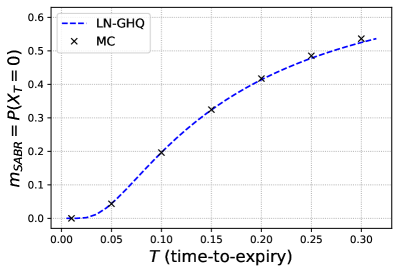
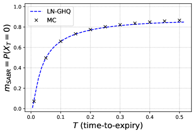
Figure 1: The mass at zero, $m_{\textsc{sabr}}$, as a function of time to maturity, $T$. We test $(x_{0},y_{0},\nu)=(0.03,0.6,1)$, and $\beta=0.5$ (left) and $\beta=0.3$ (right) with $n=10$ Gauss–Hermite quadrature points.

We demonstrate the performance of our method with numerical examples. For accuracy benchmarking, we implement the Monte-Carlo method as well. We draw random values of $V$ by simulating the paths of $Y_{t}$ over the discretized time steps and integrating the values with Simpson’s rule. In Figure 1, we redo Figure 2 of Gulisashvili et al. (2018). Figure 1 shows that the mass at zero computed with GHQ (labeled as LN-GHQ) is very close to the Monte-Carlo benchmark values (labeled as MC). This contrasts to Figure 2 of Gulisashvili et al. (2018) where the ‘LN approx’ label shows significant deviation from the ‘Exact’ label. Our method also preserves the monotonicity of the mass at zero as $T$ increases. Consequently, we do not see the need for the ‘small-time’ and ‘hybrid’ approaches introduced in Gulisashvili et al. (2018). The convergence of the GHQ is known to be very fast. We use merely $n=10$ GHQ points for Figure 1. The errors from the converged values, evaluated with $n=100$, are in the orders of $10^{-9}$ and $10^{-7}$, respectively, for the two examples. See also Choi and Wu (2019) for another numerical example and comparisons with other methods estimating the mass at zero.

3 Option Price as an Integral of the CEV Option Price

Moreover, we can similarly evaluate the option price under the SABR model. Using the GHQ, the price in Eq. (3) can be approximated by the weighted sum of the CEV option prices in Eq. (2):

$$C_{\textsc{sabr}}(y_{0},\nu)\approx\sum_{k=1}^{n}w_{k}C_{\textsc{cev}}(y_{0}\sqrt{v_{k}})\quad\text{for}\quad v_{k}=\mu_{1}\exp\left(\lambda z_{k}-\frac{\lambda^{2}}{2}\right).$$ (6)

This direct pricing approach has several critical advantages over the original method using the DMHJ formula. First, we can price the options for any strike price, while the DMHJ formula is accurate only for small strikes and diverges for bigger strikes. Second, the price from the new method is completely arbitrage-free because so is each of the CEV price components. Third, this approach can be applied to the lognormal ($\beta=1$) and normal ($\beta=0$) SABR models, to which the DMHJ formula is not applicable because the mass at zero is not available. In those two cases, the CEV price in Eq. (6) should be replaced by the Black–Scholes and Bachelier prices, respectively.

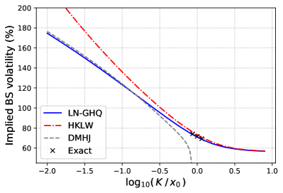
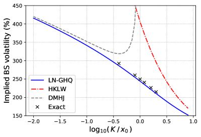
Figure 2: The Black-Scholes volatility smile as a function of log strike price for two parameter sets: $(x_{0},y_{0},\nu,\beta,T)=(0.5,0.5,0.4,0.5,2)$ (left) and $(x_{0},y_{0},\nu,\beta,T)=(0.05,0.4,0.6,0.3,1)$ (right). The mass at zero, estimated by the method of this study, are $m_{\textsc{sabr}}=0.1657$ and $0.7624$, respectively.

Figure 2 demonstrates the advantages of the direct pricing method. We examine two parameter sets tested by prior studies, von Sydow et al. (2019) and Cai et al. (2017). The exact options prices are available from the references. We also compare the HKLW formula (labeled as HKLW) as it is the industry standard. The lognormal approximation with GHQ (labeled as LN-GHQ) shows an excellent agreement with the exact implied volatilities near the money. In the second parameter set (right), the HKLW formula significantly deviates from the exact value. In the low-strike region, the volatility smile from our method is also consistent with the DMHJ formula, with estimated mass at zero, $m_{\textsc{sabr}}=0.1657$ (left) and $0.7624$ (right), respectively. These are very close from the values from the Monte-Carlo method, $m_{\textsc{sabr}}=0.1634$ (left) and $0.7758$ (right) respectively. Yet, not surprisingly, the DMHJ formula diverges near the money ($K=x_{0}$). Therefore, our new pricing method is superior to the existing method across all strike range.

Funding

Jaehyuk Choi gratefully acknowledges the financial support of the 2019 Bridge Trust Asset Management Research Fund. Lixin Wu was supported by Hong Kong RGC Grant #16306717.

References

- Abramowitz and Stegun (1972) Abramowitz, M., Stegun, I.A. (Eds.), 1972. Handbook of Mathematical Functions with Formulas, Graphs, and Mathematical Tables. New York. URL: https://www.math.hkbu.edu.hk/support/aands/toc.htm.
- Antonov et al. (2015) Antonov, A., Konikov, M., Spector, M., 2015. The free boundary SABR: Natural extension to negative rates. Risk September, 1–6.
- Antonov et al. (2019) Antonov, A., Konikov, M., Spector, M., 2019. Modern SABR Analytics. SpringerBriefs in Quantitative Finance, Cham. doi:10.1007/978-3-030-10656-0.
- Cai et al. (2017) Cai, N., Song, Y., Chen, N., 2017. Exact Simulation of the SABR Model. Operations Research 65, 931–951. doi:10.1287/opre.2017.1617.
- Choi et al. (2019) Choi, J., Liu, C., Seo, B.K., 2019. Hyperbolic normal stochastic volatility model. Journal of Futures Markets 39, 186–204. doi:10.1002/fut.21967.
- Choi and Wu (2019) Choi, J., Wu, L., 2019. The equivalent constant-elasticity-of-variance (CEV) volatility of the stochastic-alpha-beta-rho (SABR) model. arXiv:1911.13123 [q-fin] URL: http://arxiv.org/abs/1911.13123, arXiv:1911.13123.
- De Marco et al. (2017) De Marco, S., Hillairet, C., Jacquier, A., 2017. Shapes of Implied Volatility with Positive Mass at Zero. SIAM Journal on Financial Mathematics 8, 709–737. doi:10.1137/14098065X.