De-localizing brittle fracture

Abstract

Extreme localization of damage in conventional brittle materials is the source of a host of undesirable effects. We show how artificially engineered metamaterials with all brittle constituents can be designed to ensure that every breakable sub-element fails independently. The main role in the proposed design is played by high contrast composite sub-structure with zero-stiffness, furnishing nonlocal stress redistribution. The ability to de-localize cracking in such nominally brittle systems is revealed by the fact that their continuum description is dominated by the gradient (bending) rather than classical (stretching) elasticity. By engineering a crossover from brittle to effectively ductile (quasi-brittle) behavior in prototypical systems of this type, we reveal the structural underpinning behind the difference between fracture and damage.

1 Introduction

Typically brittle materials fail through the development of a macro-crack which originates from a microscopic flaw and advances by focusing singular stresses near the tip [1, 2]. Such extreme stress localization can be traced to the nonconvexity of the inter-atomic potential [3, 4] leading to softening of elastic response and attendant loss of ellipticity of equilibrium equations [5, 6]. In applications, the formation of a system spanning macro-crack is often viewed as an undesirable effect due to low resulting toughness and the catastrophic character of ensuing dynamics [7, 8].

Many ingenious strategies for tempering brittleness and creating effective ductility have been proposed in the literature, including toughening by microcracking [9, 10], engaging phase transformations [11, 12] and utilizing multi-level failure mechanisms [13, 14], to mention just a few. The usual underlying idea is to avoid the unstable crack propagation [15] by creating obstacles and dissipation centers [16, 17, 18] that can trap the system in metastable configurations [19, 20]. It was shown that such crack re-channeling mechanisms can be tailored to achieve high energy absorption and that the resulting nominally brittle artificial materials can rival their natural ductile analogs [21, 22, 23].

In this paper, we propose a different approach to fracture de-localization, which can be viewed as rigidity mitigation [24]. The underlying idea is to buttress the material’s progressive softening by strengthening the nonlocal interactions that ensure stress redistribution and prevent strain localization. The task of transmitting such interactions is assigned to a distributed floppy metamaterial sub-structure whose elasticity is bending dominated.

As a proof of principle, we present here the simplest prototype of such a mechanical system. Our clearly oversimplified model example aims to elucidate, by making analytically tractable, the transition from the conventional elastic behavior at small tensile loading (and no damage) to the bending-dominated elastic response at considerable tensile loading (and appreciable damage). We show that such transition ensures that instead of softening-induced strain localization, the system redistributes strain globally so that every single brittle sub-element breaks independently. The proposed design relies on the stabilization of floppy mechanical modes through bending rigidity. It has a bio-mimetic origin as it structurally imitates some known prototypes in living nature [25, 26]. However, such structures with variable-connectivity can now be built artificially using the existing techniques of additive manufacturing [27].

Our composite design is deliberately minimalistic as we assemble it using the most simple local and nonlocal elastic sub-structures. The local sub-structure is represented by a chain of springs with Lennard-Jones-type nonconvex potential. The nonlocal sub-structure is a zero-stiffness pantograph composed of inextensible but flexible beams connected through ideal pivots [28, 29, 30]. The two sub-structures are coupled in such a way that in the initial state, where all breakable springs are intact, the whole system is over-constrained [31, 32]. As the structure is stretched, the geometrical constraints force the breakable elements to fail, and the composite mechanical system progressively transforms into an under-constrained one with dominating bending (gradient) elasticity. While we use only a particular nonlocal sub-structure in our analysis, other floppy designs could be used as well, see for instance, [33] and examples in our concluding Section. A general analysis of the nonlocality in such systems can be found in the theory of high contrast elastic composites [34, 35]. Contrary to what is known for usual composite materials, higher-order derivatives in the homogenized representation of such systems, appear already at the leading order [36, 37, 38].

If, in the absence of a floppy reinforcement, a series of breakable springs loaded in tension fails abruptly with a formation of a single macro-crack, e.g., [39]. Instead, we show that the same system with a floppy reinforcement breaks gradually and exhibits distributed microcracking. The whole process can be interpreted as damage spreading and viewed as a propagation of a diffuse front separating affine and non-affine deformation configurations. Most remarkably, due to the presence of nonlocal reinforcement, the affine deformation is recovered at a sufficiently large stretching with strain uniformity being rebuilt by bending elasticity. Such re-entrant homogeneity of deformation distinguishes the proposed metamaterial structures from the conventional brittle solids because the latter cannot heal the acquired non-affinity in monotone loading.

We show that in the continuum framework, our metamaterial structure can be modeled as a softening elastic solid with a strain gradient term in the energy representing bending elasticity. The ensuing continuum model takes the classical Ginzburg-Landau form with macroscopic strain playing the role of order parameter [40, 41]. However, to describe fracture, the usual double-well energy has to be replaced by Lennard-Jones type potential. A model of this type was considered in [42], but under a constitutive condition which effectively erased the healing effect. Another closely related model is the strain-gradient-regularized damage mechanics [43], though in this framework, our crucial assumption that the nonlocal stiffness is damage-independent has been so far considered as unrealistic [44]. A conceptual link can also be built between our approach and models developed to describe ductile fracture in plastic solids when an effective local energy is complemented by a weakly nonlocal term describing strain gradient hardening [45, 46].

To elucidate the possibility of fracture delocalization patterns in our model we also consider a version with elastic background, particularly relevant for biological applications [47]. In this setting, the ‘effectively ferromagnetic’ interactions, implied by bending elasticity, compete with ‘effectively anti-ferromagnetic’ interactions brought by the elastic background [48]. The resulting mechanically frustrated system is shown to generate complex periodic arrangements of alternating affine and non-affine behavior.

If a nonlocal sub-structure is absent, the remaining local sub-structure represents a conventional brittle material that can be simulated in the continuum limit by gradient damage model [49, 50, 51, 52, 53] or any other phase-field model of fracture [54, 55, 56, 57]. In this setting, we show that neither damage-spreading nor re-entrant behavior takes place. Even when the elastic environment is added, the broad microcracking domains, characteristic of our metamaterial response, do not appear. Instead, we observe in this case only the conventional pattern of highly localized macro-cracks.

Our systematic comparison of the Ginzburg-Landau type elastic model with the phase-field model shows that only the former provides an adequate description of the pantograph-reinforced breakable chain. Thus, in the absence of an elastic environment, only the former generates the characteristic isola-center bifurcation when the nontrivial branch of equilibria separates from and then reconnects to the trivial branch at two distinct points [58]. Rather intriguingly, the revealed relation between these two theories in the current context (see also [44]) is rather similar to the one between the Foppl-von Karman and the fully nonlinear 3D theories of wrinkling in stretched elastic sheets [59]. The fundamental fact that the phase-field model misses the crucial re-entry effect shows that the penalization of the inhomogeneity through gradients of damage is a much weaker form of regularization than through the gradients of strain because only the latter can ensure the affine response even in the case of complete degradation of the conventional elasticity.

The rest of the paper is organized as follows. In Section 2, we introduce the discrete model of the pantograph-reinforced breakable chain and show that fracture in this system is de-localized. In Section 3, we build a continuum version of the same system and show that its mechanical response reproduces its discrete prototype’s mechanical behavior. In Section 4, we study the case when the continuum model is constrained by an elastic environment showing the emergence of regular patterns with alternating affine and non-affine strain configurations. In Section 5, we compare (at continuum level) the behavior of pantograph-reinforced and non-reinforced brittle systems. In the final Section 6, we present elementary examples of 2D systems with fracture de-localizing floppy substructures and summarize our results.

2 The design idea

To motivate further developments, consider a conventional mass-spring chain constrained to remain on a straight line, see Fig. 1. The goal of this basic pre-model is to mimic the mechanical behavior of a softening nonlinear elastic material. To this end, we assume that the springs are ‘breakable’ and that their mechanical response is described by a non-convex elastic potential of Lennard-Jones type.

Figure 1: The simplest (not reinforced) mass-spring chain. Particles are connected in series by breakable springs and the whole system is loaded in tension.

Define the horizontal displacement $u_{i}=x_{i}-x^{0}_{i}$ of the mass point with index $i$ where $x_{i}$ is its actual coordinate and $x^{0}_{i}=ai$ is its reference coordinate. The energy of this system can be written in dimensionless form

$$E_{S}({\bf u})=a\sum_{i=0}^{N-1}f\left(\frac{u_{i+1}-u_{i}}{a}\right).$$ (1)

where $a=1/(N-1)$ is dimensionless reference length. For our numerical illustrations, where we deal exclusively with tension, it will be sufficient to use an analytically convenient expression for the elastic potential $f(\varepsilon_{i})=\varepsilon_{i}^{2}/(2+\varepsilon_{i}^{2})$ where we introduce the discrete strain $\varepsilon_{i}=(u_{i+1}-u_{i})/a$, see Fig. 2.

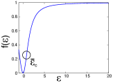
Figure 2: The elastic potential of Lennard-Jones-type describing the mechanical response of a ‘breakable’ spring loaded in tension. The compression range is not shown because it is not used in this study. The inflection point $\bar{\varepsilon}_{c}$ marks the instability of the affine response for the simplest chain with nearest neighbor interactions shown in Fig. 1.

Suppose next that the chain is stretched quasi-statically in a hard device so that $u_{0}=-\bar{\varepsilon}/2$ and $u_{N-1}=\bar{\varepsilon}/2$, were $\bar{\varepsilon}>0$ is the average strain which plays the role of loading parameter. To find the macroscopic response we need to solve for each value of $\bar{\varepsilon}$ the equilibrium equations

$$\partial{E_{S}}/\partial u_{i}=0\text{ , }1<i<N-2.$$ (2)

Knowing that continuous branches of equilibria can terminate, we need to prescribe the branch switching strategy defined by the dynamic extension of the model. Such extension should ensure that the system re-stabilizes after an instability in a dissipative way and in quasi-static setting reduces to the selection of a new locally stable equilibrium branch with necessarily lower energy. In this paper, we will compare two dynamic strategies.

Having the structural mechanics applications in view, we should be choosing the new equilibrium branch using the local energy minimizing (LEM) criterion which mimics the zero viscosity limit of an overdamped viscous dynamics. Under this protocol, the quasi-static loading will maintain the system in a metastable state (local minimum of the energy (1)) till it ceases to exist and then, during an isolated switching event, select the new equilibrium branch using the steepest descent algorithm [60].

With the biomechanical applications in view, where temperatures are different from zero and the energy scale of thermal fluctuations is comparable to the existing energy barriers, we also discuss the global energy minimizing (GEM) strategy. It implies that at each value of the loading parameter, the system is able to minimize the energy globally. Physically, this branch selection strategy indicates the parametric thermal equilibration with the subsequent zero-temperature limit. While for macroscopic engineering structures, the global energy minimization does not make much sense in the context of fracture, at sufficiently small scales (encountered, for instance, in cells and tissues) and over sufficiently large times, thermal fluctuations can be thought as exploring enough of phase space to make global minima relevant.

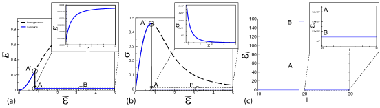
Figure 3: The LEM response of a mass-spring chain with breakable springs subjected to quasi-static tensile loading in a hard device: (a) the equilibrium elastic energy $\bar{E}_{S}(\bar{\varepsilon})$ and, (b) the equilibrium stress $\sigma(\bar{\varepsilon})=d\bar{E}_{s}/d\bar{\varepsilon}$, (c) the equilibrium strain profiles $\varepsilon_{i}(\bar{\varepsilon})$, $i=1,...,N$. Hypothetical affine response is compared with numerical simulations following the LEM protocol. Insets: (a,b) the response of the broken chain beyond point A, (c) the state of the unloaded springs in points A and B. Here $N=50$.

While for the system with energy (1) both LEM and GEM responses can be studied analytically, we use here this simple case to detail our numerical approach. For instance, in Fig. 3 we illustrate the classical brittle fracture with ultimate (lattice scale) strain localization. Here we apply the LEM strategy while stretching the chain with $N=50$. The incremental energy minimization is based on L-BFGS algorithm [61] (imitating gradient flow), which builds a positive definite Hessian approximation for (2) allowing one to make a quasi-Newton step lowering the total energy [62]. Such iterations continue till the increment in the energy becomes sufficiently small. We then use the obtained approximate solution as an initial guess $\bf w$ to solve, using LU factorization [63], the linear equations for the correction $\Delta\bf w$

$$K_{ij}\Delta w_{j}+\Delta f_{i}=0,$$ (3)

where $K_{ij}=\partial^{2}E_{S}/\partial u_{i}\partial u_{j}$ is the discrete stiffness matrix, and $\Delta f_{i}$ are the bulk forces. The displacement field is updated in this way till the gradient norm of Eq. 2 is smaller than $10^{-8}$ which furnishes the actual solution of the problem. The loading is performed by monotonically increasing the value of the displacements of boundary nodes $u_{0}=-\bar{\varepsilon}/2$ and $u_{N-1}=\bar{\varepsilon}/2$ in increments of $10^{-6}$. The Hessian matrix $K_{ij}$ is also used to assess the stability of the obtained equilibrium configurations. To determine the GEM path we simply chose at each value of $\bar{\varepsilon}$ the equilibrium configuration with the lowest energy.

In Fig. 3 we show separately the equilibrium macroscopic energy, $\bar{E}_{S}(\bar{\varepsilon})$, the equilibrium macroscopic stress $\sigma(\bar{\varepsilon})=d\bar{E}_{S}/d\bar{\varepsilon}$ and the equilibrium distribution of the microscopic strains $\varepsilon_{i}$ in individual springs. The homogeneous (affine) configuration remains locally stable till the value $\bar{\varepsilon}=\bar{\varepsilon}_{c}$ is reached, where $\bar{\varepsilon}_{c}$ is defined by the instability condition $\partial^{2}f/\partial\varepsilon^{2}=0$, see Fig. 2. As the homogeneous state becomes unstable, the stress drops to almost zero and then continues to diminish further as the loading parameter increases, see the inset in Fig. 3(b). During the stress drop, the strain abruptly localizes at the scale of the lattice, see Fig. 3(c). The location of the ensuing macro-crack is accidental and was chosen by an initial imperfection. Subsequent loading increases the crack opening while further unloading the rest of the sample, see Fig. 3(c). Under the GEM protocol, similar isolated macroscopic crack forms before the point $\bar{\varepsilon}_{c}$ is reached, see for instance, [39], however, the subsequent growth of this crack follows the same equilibrium branch as in LEM case. The main difference is that under the LEM strategy, the dissipation during the brittle failure process is finite, while under the GEM strategy the dissipation is identically zero.

After the major stress drop the subsequent loading does not create additional damage and the response reduces to the increase of the amplitude of the localized strain. Note also that during the stress drop, the system does not fully unload because some (weakening) elastic interaction between the newly formed crack lips always exists. A 1D model of brittle fracture where stress drops to zero while the boundary layers near the lips remain have been recently proposed in [64].

Figure 4: The reinforced chain of breakable springs. The pantograph floppy frame constitutes a sub-structure. The system is loaded in tension.

To de-localize brittle fracture, we now reinforce the series connection of breakable springs by adding a sub-structure whose role is to ensure that the strain is uniformly redistributed. The simplest sub-structure of this type is a pantograph frame made of inextensible but bendable beams connected by ideal pivots, see Fig. 4. While it has zero longitudinal macroscopic stiffness, (it does not resist affine deformations) the non-affine longitudinal deformations remain energetically penalized due to the finite bending rigidity of individual beams. If we again assume that the composite system shown in Fig. 4 is constrained to remain on a straight line, we can write the elastic energy of the bending beams in the form

$$E_{B}({\bf u})=a\sum_{i=1}^{N-1}\frac{\lambda_{1}^{2}}{2}\left(\frac{u_{i+1}+u_{i-1}-2u_{i}}{a^{2}}\right)^{2},$$ (4)

where $\lambda_{1}$ is a dimensionless length proportional to $a$ with the coefficient depending on the bending stiffness of the beams [65]. The total energy of the composite system is then

$$E({\bf u})=E_{S}({\bf u})+E_{B}({\bf u}),$$ (5)

where $E_{S}({\bf u})$ is given by (1). We will again load the system in a hard device with $\bar{\varepsilon}$ serving as the loading parameter. No other constraints are imposed, making the ends of the reinforced structure effectively ‘moment free’  [66].

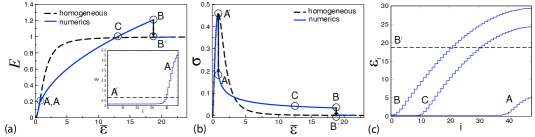
Figure 5: Mechanical response of the pantograph reinforced chain subjected to tensile loading in a hard device and following LEM dynamic protocol: (a) the equilibrium elastic energy $E(\bar{\varepsilon})$; (b) the equilibrium stress $\sigma(\bar{\varepsilon})$; (c) typical strain profiles. Inset details the transformation the homogeneous (affine) state A’ into an inhomogeneous (non-affine) state A which takes the form of the nucleation of distributed damage at the boundary of the sample. The affine state is recovered when the inhomogeneous state B, describing a developed damage zone, transforms back into the homogeneous state B’. This re-homogenization transformation would have happened at C if the system followed the global minimum path. Here, $N=50$, $\lambda_{1}=0.02236$.

The mechanical response of the pantograph-reinforced chain under the LEM protocol is illustrated in Fig. 5. To obtain the response curves, we used the same numerical approach as in the case of the non-reinforced chain. The energy minimizer is again affine at sufficiently small values of the loading parameter. At a critical value of the load (point A’) the homogeneous state becomes unstable, meaning that the corresponding local minimizer ceases to exist. The local energy minimization, imitating overdamped dynamics, produces the drop in stress and brings the system to a new local minimum (point A). However, instead of an isolated localized crack, the failure process now produces a diffuse nucleus of strain non-affinity. The strain profiles, see Fig. 5(c), suggest that the transition A’$\rightarrow$A leads to the formation of a damaged (micro-cracked) zone. The fact that it forms on one of the boundaries of the sample is a consequence of the zero moment boundary condition which effectively weakens the boundaries.

As the loading continues, the damage spreads through the structure, see the configurations C and B in Fig. 5(c). The increase of the total energy accompanies the process of successive microcracking while the stress progressively declines, see Fig. 5(b). The ‘de-localized’ failure zone advances into the sample from A to B as more and more springs get effectively broken, see Fig. 5(c). Note that the advancing zone of strain non-affinity does not have a sharp front but, instead, propagates as a diffuse wave.

According to LEM dynamics, another critical value of the loading parameter is at point B where the damage instantaneously spreads through the remaining, still-intact part of the sample, and the deformation becomes affine again all over the sample (transition B $\rightarrow$B’). This is the second dissipative event as the energy, in addition to stress, drops abruptly. The newly acquired homogeneous response remains energy minimizing at larger strains, see Fig. 5(a-c). Note that the total dissipation in this composite system, measured by the area under the resulting stress-strain curve shown in Fig. 5(b), is higher than in the case of the simple non-reinforced chain, see Fig. 3(b).

The GEM response of the pantograph-reinforced system will be roughly similar with the transition A’$\rightarrow$A taking place at smaller values of the loading parameter chosen by the corresponding Maxwell condition. Similarly, the re-stabilization of the affine state will take place earlier than under LEM protocol, at the point C, rather than B, see Fig. 5(a-c). Despite these two abrupt stress drops along the GEM path, no energy is dissipated in such a process with all the work of the loading device absorbed by the system.

We have seen that if the simplest LEM model of a breakable chain produces conventional localized fracture with an abrupt drop of stress and low dissipation, the LEM model of a pantograph-reinforced chain shows an unusual de-localized fracture with a gradual decrease of stress and higher energy dissipation. Instead of breaking into two pieces, the pantograph-reinforced chain fragments uniformly into $N$ equal pieces. The brittle response of the original system is then replaced by a ductile one with stable softening behavior and larger effective toughness. We remark that the advantages of embedding brittle elements into a compliant matrix are well known in both engineering (fiberglass) and biology (extra-cellular matrix). A certain peculiarity of our toughening mechanism is that it produces overall softening behavior instead of the more conventional hardening utilized, for instance, in ceramic matrix composites [67].

3 Continuum analog

The model shown in Fig. 4 was designed as a prototype of an inherently discrete system (metamaterial). However, such nonlinear discrete systems are not analytically transparent and therefore the origin of their unusual mechanical behavior is not apparent. Some theoretical insights can be obtained if we consider their mathematically more tractable continuum analogs.

Suppose that the (dimensionless) lattice parameter $a$ is sufficiently small. We can then look for a continuum model which, in the limit $a\rightarrow 0$, is asymptotically equivalent to our discrete model. Since the formal, scale-free asymptotic limit of the discrete theory produces a degenerate model [68, 69], we should aim at (quasi) continuum description preserving the lowest order terms in the small parameter $a$.

Approximations of different order, based on the idea of $\Gamma-$ convergence, were discussed in [70]. However, since here we are interested in local minimization of the energy, $\Gamma-$ limits are not adequate, and we need to use instead the parallel approach based on the computation of point-wise limits [71, 72]. The simplest low-order quasi-continuum approximation of this type can be obtained if we use formal asymptotic expansions of the linear finite difference operators in $a$. Using these ideas we formally replace the discrete energy functional $E({\bf u})$ in (5) by its (quasi) continuum analog

$$E(u)=\int_{0}^{1}\left(f(\varepsilon)+\frac{\lambda_{1}^{2}}{2}\varepsilon^{\prime 2}\right)dx,$$ (6)

where $\varepsilon(x)=u^{\prime}(x)$ is the continuum strain variable and $u(x)$ is the corresponding displacement field. The energy density in (6) maintains the additive structure of its discrete analog with the first term representing the stretching energy of the breakable springs and the second term describing the bending energy of the pantograph substructure. The ’redressed’ parameter $\lambda_{1}$, whose exact value will not be of interest in our qualitative study, is assumed to be strain independent given that the beams can be viewed as much stiffer than springs. It brings into the ensuing (quasi)continuum model a dimensionless length scale which does not fade away with loading as in models of un-supported mass-springs chains [42]. For numerical illustrations we continue to use the particular function $f(\varepsilon)=\varepsilon^{2}/(2+\varepsilon^{2})$.

To model the system loaded in a hard device, we again set $u(0)=-\bar{\varepsilon}/2$, $u(1)=\bar{\varepsilon}/2$ where $\bar{\varepsilon}>0$ is the imposed strain. Given that the boundaries are moment free, we also use the natural higher order boundary conditions $u^{\prime\prime}(0)=u^{\prime\prime}(1)=0.$ Under these assumptions the homogeneous (affine) configuration $u^{0}(x)=(\bar{\varepsilon}/2)(2x-1)$ is an equilibrium state at all values of the loading parameter $\bar{\varepsilon}$.

Due to the softening nature of the energy density $f$, the homogeneous configuration can be expected to become unstable in tension. To find the critical value of the loading parameter we need to study the linear problem for the perturbation $s(x)=u(x)-u^{0}(x)$

$$-\lambda_{1}^{2}s^{\prime\prime\prime\prime}+\frac{\partial^{2}f}{\partial\varepsilon^{2}}(\bar{\varepsilon})s^{\prime\prime}=0,$$ (7)

with the boundary conditions $s(0)=s(1)=s^{\prime\prime}(0)=s^{\prime\prime}(1)=0.$ The system becomes linearly unstable when the second variation of the energy (6) loses its positive definiteness and the problem (7) acquires a nontrivial solution. The largest eigenvalue of the linear operator with constant coefficients in the left hand side of (7) is $-\lambda_{1}^{2}\pi^{4}-(\partial^{2}f/\partial\varepsilon^{2})(\bar{\varepsilon})\pi^{2}$ and the corresponding eigenvector is $s(x)\sim\sin(\pi x)$ [73, 74]. Therefore, the homogeneous solution is stable for $(\partial^{2}f/\partial\varepsilon^{2})(\bar{\varepsilon})>-\lambda_{1}^{2}(\pi)^{2}$ and the loss of stability takes place at the smallest $\bar{\varepsilon}$ such that $(\partial^{2}f/\partial\varepsilon^{2})(\bar{\varepsilon})=-\lambda_{1}^{2}\pi^{2}$. The higher order modes $s(x)\sim\sin(n\pi x)$ with $n>1$ bifurcate at the values of the loading parameter satisfying

$$\frac{\partial^{2}f}{\partial\varepsilon^{2}}(\bar{\varepsilon})=-\lambda_{1}^{2}(n\pi)^{2}.$$ (8)

The corresponding stability boundaries, representing solutions of (8) at different values of $n$ and $\lambda_{1}$, are illustrated in Fig. 6(a,b) for the case of our special $f(\varepsilon)$. In Fig. 6(a,b) we show that, independently of the value of the parameter $\lambda_{1}$, the wavelength of the critical perturbation always corresponds to $n_{c}=1$.

Note a remarkable feature of the stability diagrams shown in Fig. 6(a,b). If $\lambda_{1}$ is sufficiently small, the homogeneous (affine) configuration is stable in the two disconnected domains: when the applied stretch is sufficiently small $\bar{\varepsilon}\leq\bar{\varepsilon}_{c}^{*}$ and when it is sufficiently large $\bar{\varepsilon}\geq\bar{\varepsilon}_{c}^{**}$, with the same critical mode number ($n_{c}=1$) responsible for both instabilities, see Fig. 6(c). This observation points to the existence of the re-entrant behavior characteristic for the isola-center bifurcations [75, 58, 76]. When the dimensionless parameter $\lambda_{1}$ is sufficiently large (large bending modulus or small system size), the affine configurations are stable in the whole range of loadings. In such ‘overconstrained’ regimes, failure becomes ‘dissipationless,’ taking place gradually and uniformly throughout the whole system.

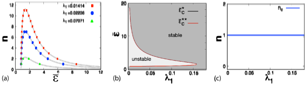
Figure 6: Linear stability boundaries for the homogeneous state in the continuum model of pantograph-reinforced chain: (a) bifurcation points, (b) critical strains $\bar{\varepsilon}_{c}^{*}$ and $\bar{\varepsilon}_{c}^{**}$ bounding the unstable domain (c) critical wavenumber $n_{c}$ vs $\lambda_{1}$.

The metastable non-affine configurations can be found by solving the nonlinear equilibrium equation

$$-\lambda_{1}^{2}u^{\prime\prime\prime\prime}+\frac{\partial^{2}f}{\partial\varepsilon^{2}}(u^{\prime})u^{\prime\prime}=0,$$ (9)

with the chosen boundary conditions for $u(x)$. The whole set of solutions of the nonlinear equation (9) can be obtained in quadratures, e.g., [73, 74, 77]. For the general problem with an arbitrary convex-concave potential $f(\varepsilon)$, different equilibrium branches can be parametrized by the unstable wave number $n$ at the point of bifurcation from the trivial homogeneous solution; the latter itself can be associated with $n=0$. One can show that all branches $u_{n}(x)$ with $n>1$ are all unstable [78, 73, 74]. It can be also shown that the branch with $n=1$ which bifurcates from the trivial homogeneous branch of equilibria at $\bar{\varepsilon}_{c}^{*}$ does it subcritically and that it reconnects to it at $\bar{\varepsilon}_{c}^{**}$ also subcritically [74].

These general observations are confirmed numerically in the case of our special potential $f(\varepsilon)$, see Fig. 7(a) and Fig. 8(a,b). Equilibrium branches were found using a pseudo-arclength continuation technique, implemented in the software AUTO [79]. It solves the nonlinear equation Eqs. 9 with the relative end displacement treated as a continuation parameter. To discretize the boundary-value problem, it uses collocation with Lagrange polynomials, and in our simulations, we had $N=200$ mesh points with $N_{c}=5$ collocation nodes and activated mesh adaptation. To study stability we checked numerically the positive definiteness of the second-variation

$$\delta^{2}E(u)(v,v)=\int_{0}^{1}[(\partial^{2}f/\partial\varepsilon^{2})(u^{\prime})v^{\prime}v^{\prime}+\lambda_{1}^{2}v^{\prime\prime}v^{\prime\prime}]dx,$$ (10)

where $v$ are the test functions respecting the boundary conditions. We discretized the integral (10) to construct the stiffness matrix ${\bf K}$ and then investigated numerically the sign of the minimal eigenvalue $\kappa$ of the corresponding finite quadratic form [63]. To this end, we used one-dimensional finite elements based on third-order polynomial shape functions containing four unknown constants (cubic Hermite interpolation) [80]. This implies that four shape functions were used in each two-node element (4 degrees of freedom), and we used a uniform mesh with an element size $h_{e}=1/1000$. The discrete solution $u^{\prime}(x_{i})$ provided at discrete nodes $x_{i}$ by AUTO was first interpolated using B-spline basis function of degree 3  [81] and then used to calculate the integral 10 using a three-point Gauss integration scheme; the fixed boundary conditions were imposed by removing from the stiffness matrix ${\bf K}$ the row and columns at $x=0$ and $x=1$. As a result, the second variation (10) was approximated by a finite sum with $K_{ij}=\int_{0}^{1}[(\partial^{2}f/\partial\varepsilon^{2})(u^{\prime}){\mathcal{N}}^{\prime}_{i}{\mathcal{N}}^{\prime}_{j}+\lambda_{1}^{2}{\mathcal{N}}^{\prime\prime}_{i}{\mathcal{N}}^{\prime\prime}_{j}]dx,$ where ${\mathcal{N}}_{i}(x)$ is the shape function of node $i$ [80].

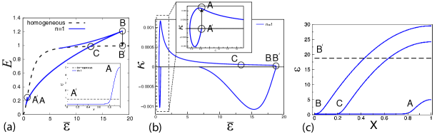
Figure 7: The LEM mechanical response in tensile loading for the continuum model of a pantograph reinforced chain: (a) equilibrium energy-strain relation for the branch $n=1$ with the lowest energy, (b) smallest eigenvalue of the second variation for the mode $n=1$ as a function of the loading parameter $\bar{\varepsilon}$. The inset in (a) shows the nucleation of the diffuse damage zone near the boundary of the sample (transition A’$\rightarrow$A). In point B the non-affine state transforms into the affine state (transition B$\rightarrow$B’). Along the global energy minimization path (GEM response) the re-entry type transformation would take place in point C. Here $\lambda_{1}=0.02236.$

In Fig. 7(a) we show the macroscopic energy-strain relation for the system following the LEM protocol. The non-affine branch with $n=1$ bifurcates from the trivial branch at point A’. Since the bifurcation is subcritical, the system jumps from the homogeneous state A’ to the inhomogeneous state A located on the only other stable equilibrium branch (with $n=1$), see the inset in Fig. 7(a). During this abrupt transition, the stress drops, and the energy is dissipated, see Fig. 8(b). As the loading parameter increases, the system follows the $n=1$ branch till it reaches the turning point B. From there the system abruptly returns to the homogeneous (affine) branch $n=0$ as a result of a dissipative transition accompanied with another stress drop, see Fig. 8(b). Further loading preserves the affine nature of the strain configuration which has recovered its stability. In Fig. 7(b) we show the strain dependence of the lowest eigenvalue of the second variation $\kappa$ for the equilibrium branch with $n=1$. As we see, this branch bifurcates from the branch with $n=0$ at the point A’ as an unstable one. However, the non-affine state A, where the LEM solution jumps, is stable as the corresponding $\kappa>0$. The branch $n=1$ loses stability again at the turning point B where $\kappa=0$.

We remark that the global structure of the nontrivial branch $n=1$ is similar to the one obtained in the Ginzburg-Landau model with a double-well potential, e.g. [73]. The same topological structure of the bifurcation diagram is observed in a model with a single-well potential because the separation and the reconnection of the nontrivial branch $n=1$ with the trivial branch $n=0$ takes place outside the energy wells, in the spinodal region, which is effectively present in both types of theories.

The structure of the associated local energy minimizers is illustrated in Fig. 7(c). The abrupt nucleation of the first domain of non-affinity takes place at the point A’ corresponding to $\bar{\varepsilon}_{c}^{*}>\bar{\varepsilon}_{c}$. In the linear regime, the unstable bifurcating mode has a characteristic size of the system, but in the nonlinear regime, it partially localizes near one of the boundaries (transition A’$\rightarrow$A). As the applied strain $\bar{\varepsilon}$ increases, the non-affine state of distributed damage proliferates towards the other boundary of the sample; note that it remains diffuse as successive springs continue to break. Observe broad transition layers, separating the non-affine domains which contain broken springs (domains where $\partial^{2}f/\partial\varepsilon^{2}<0$) and the dominating elasticity is of the bending (gradient) type, from the affine domains which contain intact springs (domains where $\partial^{2}f/\partial\varepsilon^{2}>0$) and the dominating elasticity is of the classical ’stretching’ type. The fully affine configuration is recovered through the discontinuous event which marks the complete annihilation of the stretching dominated domain (transition B$\rightarrow$B’).

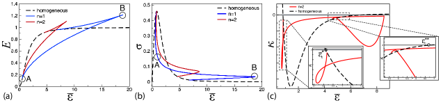
Figure 8: The mechanical response in the continuum model of a pantograph reinforced chain : (a) equilibrium energy-strain relations showing the two lowest energy branches, (b) the corresponding stress-strain relations, (c) minimal eigenvalues of the second variation for branches with $n=0$ (homogeneous) and $n=2$ (unstable).

Since branches with $n=0$ and $n=1$ are the only ones containing stable fragments, the GEM path can also be read off our Fig. 7(a). Thus, the global energy minimizing transition from $n=0$ to $n=1$ branch takes place slightly before point A’ while the reverse transition occurs at point C. It involves the instantaneous breaking of almost half of the springs and precedes considerably the analogous transition in the LEM model taking place at the point B, see Fig. 7(c).

An unstable equilibrium branch with $n=2$, which does not participate in either LEM, or GEM paths, is illustrated in Fig. 8. It describes saddle points but exhibits similar isola-center bifurcation. The instability of this branch is illustrated Fig. 8(c) where we show the strain dependence of the lowest eigenvalue of the second variation $\kappa$ for branches with $n=0$ and $n=2$. Note that since the $n=2$ branch bifurcates from the trivial state as the second eigenvalue of the second variation becomes negative, the curve $\kappa(\bar{\varepsilon})$ in Fig. 8(c) corresponding to $n=2$ originates on $n=1$ branch rather than $n=0$ branch. It is also clear from Fig. 8(a) that the branch $n=2$ corresponds to a higher energy level than the branch $n=1$ and, therefore, independently of the local stability analysis, it cannot make appearance in principle along the GEM path.

Our analysis shows that the behavior of the (quasi)continuum model is qualitatively similar to the behavior of the corresponding discrete model, compare Fig. 5 and Fig. 7. In particular, both models predict the abrupt emergence and subsequent proliferation of the non-affinity zones which contain inhomogeneously ruptured springs. Similarly, both models predict the abrupt recovery of the affine state as the rupture process saturates.

Note that the non-affine states, stabilized by bending (gradient) elasticity, can be characterized at the macro-scale in terms of damage mechanics. It provides a homogenized description of de-localized microcracking which is relevant when the competing localized macro-cracking is inhibited. The nonlocal stress redistribution, facilitated by an under-constrained sub-system of stress-transmitting backbones, may be considered a factor contributing to such inhibition.

4 Elastic background

To show that the de-localized damage can also appear in the form of periodic patterns, we now consider our pantograph-reinforced chain coupled to an elastic (Winkler’s) background. Breakable networks embedded in soft elastic matrices are structural elements in many engineering materials and biological materials, see for instance, [82, 83, 84].

To achieve analytical transparency, we again assume that the parameter $a$ is sufficiently small and adopt the quasi-continuum description encapsulated in (6). Under the simplifying assumption that the elastic background is uniformly pre-stretched with the same strain $\bar{\varepsilon}$ as the composite chain, we can write the energy of the system in the form [85, 86]

$$E(u)=\int_{0}^{1}\left(f(\varepsilon)+\frac{\lambda_{1}^{2}}{2}\varepsilon^{\prime 2}+\frac{\lambda_{2}^{-2}}{2}(u-u^{0})^{2}\right)dx,$$ (11)

where $u^{0}(x)=(\bar{\varepsilon}/2)(2x-1)$ and $\lambda_{2}$ is a new dimensionless length scale characterizing the strength of the coupling; note that in (11) the elastic energy of the background is effectively subtracted. In what follows, we use the same boundary conditions on $u(x)$ as in the case of the unsupported chain.

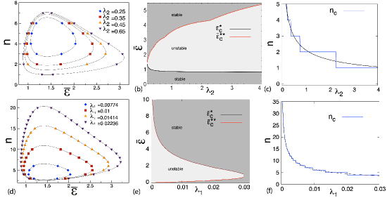
Figure 9: Linear stability limits for the homogeneous state in the continuum model of pantograph reinforced chain coupled to an elastic background: (a,d) bifurcation points, (b,e) critical strains $(\bar{\varepsilon}_{c}^{*},\bar{\varepsilon}_{c}^{**})$; (c,f) critical modes $n_{c}$. Parameters: in (a-c) $\lambda_{1}=0.02236$. In (d-f) $\lambda_{2}=0.25$.

In the model with energy (11), the bifurcation condition for the trivial branch can be found from the equation generalizing (8)

$$\lambda_{1}^{2}(n\pi)^{4}+\frac{\partial^{2}f}{\partial\varepsilon^{2}}(\bar{\varepsilon})(n\pi)^{2}+\lambda_{2}^{-2}=0.$$ (12)

We again obtain that there are upper and lower critical strains $\bar{\varepsilon}_{c}^{*}$ and $\bar{\varepsilon}_{c}^{**}$ corresponding to the same mode number $n_{c}$ so the bifurcation from the trivial branch is always of isola-center type. The difference from the case without the foundation is that now one can have $n_{c}\neq 1$, see Fig. 9. To interpolate critical thresholds we neglect the discreteness and write the approximating relations $\partial^{2}f/\partial\varepsilon^{2}({\bar{\varepsilon}_{c}})=-2(\lambda_{1}/\lambda_{2})$ and $n_{c}=\pi^{-1}(\lambda_{1}\lambda_{2})^{-1/2}$. The expression for the critical wavenumber suggests that the instability is of Turing type [87, 88].

The dependence of solutions of (12) on parameters $\lambda_{1}$ and $\lambda_{2}$ is illustrated in Fig. 9(a,d); the parametric dependence of the corresponding bifurcation thresholds $\bar{\varepsilon}_{c}^{*}$ and $\bar{\varepsilon}_{c}^{**}$ is shown in Fig. 9(b,e). One can see that the non-affinity can be suppressed if the bending rigidity $\lambda_{1}$ is sufficiently large or if $\lambda_{2}$ and the foundation coupling is stiff. However, the effect of the bending in this respect is much stronger than the effect of the coupling, which needs to be infinitely stiff to eliminate non-affinity completely. Note also that the wave number of the unstable mode tends to zero when either $\lambda_{1}$ or $\lambda_{2}$ disappears, see Fig. 9(c,f). Interestingly, the whole configuration of the boundaries in Fig. 9(a,d) strongly resembles similar diagrams appearing in the fully nonlinear 3D theories of wrinkles in stretched elastic sheets [59].

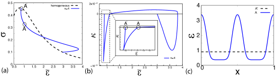
Figure 10: Mechanical response in the continuum model of pantograph reinforced chain coupled to an elastic background: (a) strain-stress relation along the first unstable branch $n=4$; (b) the smallest eigenvalue of the second variation for the same branch as a function of the loading parameter $\bar{\varepsilon}$; (c) equilibrium strain profiles associated with the states A’ and A. Parameters: $\lambda_{1}=0.0167$, $\lambda_{2}=0.45$.

The study of the post-bifurcational behavior is based on the nonlinear equilibrium equation

$$\centering-\lambda_{1}^{2}u^{\prime\prime\prime\prime}+\frac{\partial^{2}f}{\partial\varepsilon^{2}}(u^{\prime})u^{\prime\prime}-\lambda_{2}^{-2}(u-u^{0})=0.\@add@centering$$ (13)

Eq. (13) describes the interplay between the localization tendency due to nonconvexity of the energy $f(u^{\prime})$ and the delocalizing effect of weakly nonlocal bending elasticity brought by the pantograph reinforcement. This competition is in turn affected by the bias towards homogeneity brought by the interaction with an elastic foundation. The two harmonic reinforcements can be compared in terms of the effective interaction kernels [86]. Thus, the pantograph sub-structure brings sign-definite, ferromagnetic-type interaction favoring coarsening of the damaged microstructure. Instead, the Winkler’s foundation brings a sign indefinite, anti-ferromagnetic type interaction favoring microstructure refinement. The complexity of the emerging post-bifurcation behavior reflects the general frustration due to the presence of these competing tendencies.

Since the solution of (13) in quadratures is not available, we need to resort to numerical methods. Our computational approach is the same as in the case without foundation and is based on the use of the AUTO continuation algorithm [79]. The stability of equilibrium branches is again assessed by the numerical evaluation of the smallest eigenvalue of the second variation, which is now

$$\delta^{2}E(u)(v,v)=\int_{0}^{1}[(\partial^{2}f/\partial\varepsilon^{2})(u^{\prime})v^{\prime}v^{\prime}+\lambda_{1}^{2}v^{\prime\prime}v^{\prime\prime}+\lambda_{2}^{-2}vv]dx.$$ (14)

The corresponding stiffness matrix is $K_{ij}=\int_{0}^{1}[(\partial^{2}f/\partial\varepsilon^{2})(u^{\prime}){\mathcal{N}}^{\prime}_{i}{\mathcal{N}}^{\prime}_{j}+\lambda_{1}^{2}{\mathcal{N}}^{\prime\prime}_{i}{\mathcal{N}}^{\prime\prime}_{j}+\lambda_{2}^{-1}{\mathcal{N}}_{i}{\mathcal{N}}_{j}]dx.$

Our first illustration concerns the nucleation event at $\bar{\varepsilon}=\bar{\varepsilon}_{c}^{*}$. The bifurcated equilibrium branch, corresponding to $n=4$, is shown in Fig. 10(a). One may expect the instability at the point A’ to result in the transition A’$\rightarrow$A where the non-affine configuration A also lies on the $n=4$, see Fig. 10(c). However, the study of the smallest eigenvalue of the second variation (14) for the equilibrium branch $n=4$shows that the corresponding state A at $\bar{\varepsilon}=\bar{\varepsilon}_{c}^{*}$ is unstable, see Fig. 10(b). According to this figure there is a finite gap separating the first point of instability of the homogeneous state and the first stable equilibrium with $n=4$, see point A in Fig. 10(a,b).

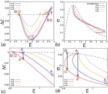
Figure 11: Mechanical response in the continuum model of a pantograph reinforced chain coupled to an elastic foundation: (a) the energy difference between the non-affine and affine equilibrium configurations; (b) macroscopic strain-stress relations along different equilibrium branches; (c,d) magnified versions of (a) and (b) near the first instability point. The transition A’$\rightarrow$A^∗ takes place along the LEM path while the transitions G’$\rightarrow$G,C’$\rightarrow$C, B’$\rightarrow$B and F$\rightarrow$F’ are the equilibrium branch switching events taking place along the GEM path. Parameters: $\lambda_{1}=0.0167$, $\lambda_{2}=0.45$.

The presence of competing interactions in this problem suggests that the stable pattern, emerging from the decomposition of the homogeneous state, may be different from the one implied by the linear stability analysis. The global picture is presented in Fig. 11(a,c) where we show the energy-strain and the stress-strain relations along the equilibrium branches with $n=3,...,6$. They all bifurcate from the homogeneous branch around $\bar{\varepsilon}_{c}^{*}=0.897334$, for instance the second bifurcation point (after the one with $n=4$) at $\bar{\varepsilon}_{c}=0.903472$ corresponds to the branch with $n=3$.

The detailed picture is shown in Fig. 11(b,d) where we see that, in view of the instability of the $n=4$ branch in the interval of interest, the only configuration reachable from point A’ by energy minimization is the one corresponding to point A^∗ on the $n=3$ branch. The local stability of this branch is illustrated in the inset in Fig. 12(c). Moreover, in this range of strains, the equilibrium branch with $n=3$ also delivers the global minimum of the energy.

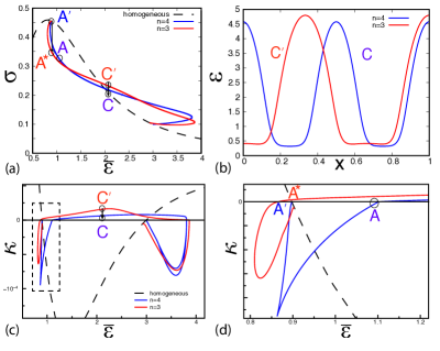
Figure 12: Zoom in on the particular branch switching events along LEM and GEM paths shown in Fig.11: (a) stress-strain response, (b) equilibrium configurations C and C’ with the same energy, (c) smallest eigenvalue of the second variation for the branches with $n=3$ and $n=4$, (d) zoom in on (c) around the first instability along the LEM path. Symmetry is lost during the transition A’ $\rightarrow$ A^∗ while symmetry is acquired during the C’$\rightarrow$C transition. Parameters: $\lambda_{1}=0.0167$, $\lambda_{2}=0.45$.

Figure 13: Zoom in on the particular branch switching events along LEM and GEM paths shown in Fig. 11: (a) stress-strain response, (b) equilibrium configurations B and B’ with the same energy, (c) smallest eigenvalue of the second variation for the branches with $n=3$ and $n=4$, (d) zoom in on (c) around the transition B’$\rightarrow$B along the GEM path. Symmetry is lost during the B’$\rightarrow$B transition. Parameters: $\lambda_{1}=0.0167$, $\lambda_{2}=0.45$.

Considering GEM dynamics, we can conclude that the transition from the trivial branch $n=0$, taking place at the point G (Fig. 11), also leads to the branch with $n=3$. According to Fig. 11(a,c) the next transition along the GEM path takes place at point C’ and brings the system back to $n=4$ equilibrium branch. Then, at point B’ the system returns again on the $n=3$ branch and finally stabilizes on the trivial $n=0$ branch at point F. In Fig. 12(b) and Fig. 13(b) we provide evidence that these GEM transitions are between locally stable states.

Our Fig. 12(c) and Fig. 12(c) illustrate the nature of the restructuring of the equilibrium configurations during these transitions. Thus, as the loading parameter $\bar{\varepsilon}$ increases, the non-symmetric configuration produced at point G, which contains two domains of non-affinity and corresponds to the branch with $n=3$, evolves till another strain threshold is reached where the system undergoes the transformation C’$\rightarrow$ C to the symmetric configuration corresponding to $n=4$. As a result, the second surface-bound damage zone appears, see Fig. 12(c). Then, during the reverse transition B’$\rightarrow$B the symmetry is lost and one of the surface-bound damage zone disappears again, see Fig. 13(c). Finally, the symmetry is recovered when the affine configuration stabilizes at point F.

In contrast to the complexity of the GEM path, the LEM dynamics produces much simpler set of transitions. Without going into details, we only mention that after the dissipative A$\rightarrow$A^∗ transition the system remains on the $n=3$ branch all the way till its reaches the turning point where another dissipative transition to the homogeneous branch $n=0$ takes place (not shown in either of the figures).

Note that the parameters in Fig. 11, Fig. 12 and Fig. 13 were chosen arbitrarily with the only consideration that the number of the domains of nonaffinity is relatively small. It is straightforward to see that the microcracking pattern in this problem may be arbitrarily complex, for instance in the limit $\lambda_{1}\rightarrow 0$ the number of cracks tends to infinity. In fact, by choosing the bending resistance of the metamaterial sub-structure and the degree of coupling with the elastic environment, one can effectively control the complexity of the emerging microstructures.

More generally, the above analysis shows that, despite the constituents’ brittle nature, the material response of the pantograph-reinforced chain is incompatible with the conventional scenario of highly localized cracking. Instead, the model predicts the emergence of de-localized damage zones, which, in the presence of elastic background, advance from multiple sources and form regular patterns. Competitive interactions ensure that a monotonously loaded system experiences a series of instabilities where symmetries may be lost and re-acquired. The interplay between two internal length scales in this problem may be a source of the considerable complexity in the spatial distribution of damage.

5 Conventional brittle fracture

Since one internal length scale is also present in the conventional fracture mechanics and another one can be added through the coupling to an elastic foundation, one may ask if the pantograph-based sub-structure brings anything fundamentally different. To answer this question we consider in this Section a continuum model of fracture where cracks are described by a phase-field [56, 52, 89].

In phase-field theories of fracture, elasticity of the breaking solid is usually assumed to be linear with stiffness degrading with damage. The latter is described by a scalar order parameter with the square of the gradient of this parameter controlling the energy cost of the the damage non-affinity [49].

Suppose that the damage variable is $\alpha(x)$ with $\alpha=0$ ($\alpha=1$) corresponding to the unbroken (fully broken) state. In the absence of the elastic environment, we can write the energy of the system in the form

$$E(u,\alpha)=\int_{0}^{1}\left(f(\varepsilon,\alpha)+\frac{\lambda_{1}^{2}}{2}(\alpha^{\prime})^{2}\right)dx.$$ (15)

where again $\varepsilon(x)=u^{\prime}(x)$. We assume that the local energy density in (15) is of the form

$$f(\varepsilon,\alpha)=\frac{1}{2}g(\alpha)\varepsilon^{2}+h(\alpha),$$ (16)

where the first term on the right, which is quadratic in strain $\varepsilon(x)$, describes linear elasticity at constant damage. The second term, depending only on $\alpha(x)$, is the energetic price of homogeneous damage. The gradient term in (15) penalizes the inhomogeneity of the damage and brings into the theory an internal length scale $\lambda_{1}$. The equilibrium branches in this model are represented by solutions of the nonlinear equations

$$\begin{cases}-(g(\alpha)u^{\prime})^{\prime}&=0\\ -\lambda_{1}^{2}\alpha^{\prime\prime}+\frac{1}{2}\frac{\partial g}{\partial\alpha}(u^{\prime})^{2}+\frac{\partial h}{\partial\alpha}&=0\end{cases}$$ (17)

To mimic in this framework our numerical experiments with the breakable chain, see Fig. 1, we make the standard assumptions that $g(\alpha)=(1-\alpha)^{2}$, and $h(\alpha)=\alpha^{2}$. if we also choose the boundary conditions in the form $u(0)=-\bar{\varepsilon}/2$, $u(1)=\bar{\varepsilon}/2$ and $\alpha^{\prime}(0)=\alpha^{\prime}(1)=0,$ the homogeneous solution, representing in this case the principal branch of equilibria, takes the form

$$u^{0}(x)=(\bar{\varepsilon}/2)(2x-1),\,\,\alpha^{0}(x)=\bar{\varepsilon}^{2}/(2+\bar{\varepsilon}^{2}).$$ (18)

The effective elastic energy along the trivial branch is

$$f^{0}(\varepsilon)=f(\varepsilon,\alpha^{o}(\varepsilon))=\varepsilon^{2}/(2+\varepsilon^{2}).$$ (19)

whose similarity with potential adopted in the study of our Ginzburg-Landau elastic model justifies the assumptions for $g(\alpha)$ and $h(\alpha)$. We may therefore perceive the phase-field model as a version of an elastic theory with the softening energy $f^{0}(\varepsilon)$ [90].

To test the linear stability of the homogeneous solution (19) we linearize (17) and look for nontrivial solutions $s(x)=u(x)-u^{0}(x)$ and $\tau(x)=\alpha(x)-\alpha^{0}$. Following the same procedure as in the previous sections, we obtain that the unstable modes are $s(x)\sim\sin(n\pi x)$ and $\tau(x)\sim\cos(n\pi x)$ with the bifurcation condition taking the form

$$(n\pi)^{2}=-\frac{4\bar{\varepsilon}^{2}\partial^{2}f^{0}/\partial\varepsilon^{2}(\bar{\varepsilon})}{\lambda_{1}^{2}[(\partial f^{0}/\partial\varepsilon(\bar{\varepsilon}))\bar{\varepsilon}-\partial^{2}f^{0}/\partial\varepsilon^{2}(\bar{\varepsilon})]}.$$ (20)

In Fig. 14(a) we illustrate the $\lambda_{1}$ dependence of the solutions of (20). As in the case of pantograph-reinforced chain, the critical mode is always $n_{c}=1$, see Fig. 14(c).

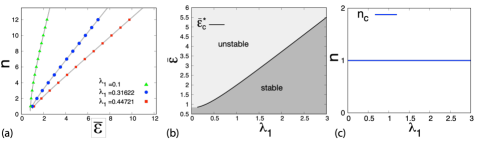
Figure 14: Stability study of the homogeneous (affine) state in the phase-field model of a unreinforced breakable chain: (a) stability boundaries (bifurcation points) depending on the regularization parameter $\lambda_{1}$; (b) critical strains $\bar{\varepsilon}_{c}$; (c) critical mode $n_{c}$.

To see the difference, we now consider the $\lambda_{1}$ dependence of the critical strain $\bar{\varepsilon}_{c}$ which can be found from the equation

$$\bar{\varepsilon}_{c}(4\bar{\varepsilon}_{c}^{2}-\lambda_{1}^{2}\pi^{2})\frac{\partial^{2}f^{0}/\partial\varepsilon^{2}(\bar{\varepsilon}_{c})}{\partial f^{0}/\partial\varepsilon(\bar{\varepsilon}_{c})}+\lambda_{1}^{2}\pi^{2}=0.$$ (21)

It takes particularly simple form for our choice of the potential $f^{0}(\varepsilon)$ when we can write $\lambda_{1}^{2}\pi^{2}=3\bar{\varepsilon}_{c}^{2}-2$, see Fig. 14(b). Now, in contrast to the case of the pantograph-reinforced chain, see Fig. 4, the affine configuration does not re-stabilizes after the initial instability and the ’broken’ configuration always remains non-affine, see Fig. 14(b). Such response is in full agreement with the behavior of a simple breakable chain, see Fig. 1, but despite the presence of gradient term in (15), the effect of the pantograph reinforcement is lost.

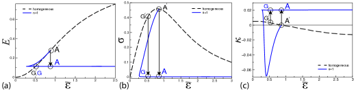
Figure 15: Mechanical response in the phase-field model of unreinforced chain along the LEM (A’ $\rightarrow$A transition) and the GEM (G’ $\rightarrow$G transition) loading paths: (a) macroscopic energy-strain relation; (b) macroscopic stress-strain relation; (c) smallest eigenvalue of the second variation for the homogeneous branch as a function of the loading parameter $\varepsilon$. Single macroscopic crack nucleation takes the form of A’$\rightarrow$A transition. Here, $\lambda_{1}=0.158114$.

The fracture localization (vs de-localization) in the phase-field model is illustrated in Fig. 15. We combine there the solutions of the nonlinear system (17) corresponding to LEM and GEM protocols. To confirm the local stability of the configurations found by our LEM algorithm, we computed the lowest eigenvalue of the second variation

$$\delta^{2}E(u,\alpha)(v,w)=\int_{0}^{1}[(1-\alpha)^{2}v^{\prime 2}-4(1-\alpha)u^{\prime}v^{\prime}w+(2+u^{\prime 2})w^{2}+\lambda_{1}^{2}w^{\prime 2}]dx,$$ (22)

where $v$ and $w$ are test functions. The stiffness matrix is then

$${\bf K}=\begin{bmatrix}\int_{0}^{1}[(1-\alpha)^{2}{\mathcal{N}}^{\prime}_{i}{\mathcal{N}}^{\prime}_{j}]dx&-2\int_{0}^{1}(1-\alpha)u^{\prime}{\mathcal{N}}^{\prime}_{i}{\mathcal{N}}_{j}dx\\ -2\int_{0}^{1}(1-\alpha)u^{\prime}{\mathcal{N}}_{i}{\mathcal{N}}^{\prime}_{j}dx&\int_{0}^{1}[(2+u^{\prime 2}){\mathcal{N}}_{i}{\mathcal{N}}_{j}+\lambda_{1}^{2}{\mathcal{N}}^{\prime}_{i}{\mathcal{N}}^{\prime}_{j}]dx\end{bmatrix},$$ (23)

where the shape functions ${\mathcal{N}}_{i}(x)$ can be now chosen simply quadratic.

According to Fig. 15, the LEM dynamics, which reduces to local energy minimization, is characterized by a major dissipative event in the form of the transition A’ $\rightarrow$A from the branch $n=0$ to the branch $n=1$. Instead, the GEM dynamics, which implies global energy minimization, is epitomized by an earlier and smaller non-dissipative transition G’ $\rightarrow$G, also from the branch $n=0$ to the branch $n=1$. Note that the metastable section of the non-affine equilibrium branch $n=1$ in Fig. 15 was constructed using again the pseudo-arclength continuation technique implemented in the software package AUTO [79].

We observe, see Fig. 15(a,b), that the stretching response of this continuum system is basically the same as for the simple chain with breakable elements. The fact that the crack forms on one of the boundaries is due to a small bias provided by the phase-field related boundary conditions. After the major stress drop the subsequent loading does not create additional damage and the response reduces to the increase of the amplitude of the localized strain. Note again that during the stress drop, the system does not fully unload because some (weakening) elastic interaction between the newly formed crack lips always exists. The noteworthy difference between the behavior of the original discrete system and its phase-field analog is the smearing out of the crack due to the gradient regularization, see Fig. 16(a,b). If the strain remains sufficiently localized, the damage parameter shows an extended boundary layer whose structure, however, is fundamentally different from the diffuse damage configuration generated in the pantograph-reinforced chain.

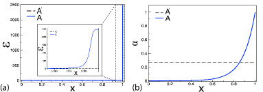
Figure 16: The detailed picture of the A’$\rightarrow$A transition shown in Fig. 15. The macroscopic crack is nucleated near the boundary of the sample: (a) strain profile, (b) damage parameter profile (b). Here, $\lambda_{1}=0.158114$.

Our example shows that the phase-field framework cannot be used alone to build a continuum model of the pantograph-reinforced structure. In particular, we show that due to weaker regularization through $\alpha$ vs regularization through $\varepsilon$, the standard phase-field model does not capture the reentry nature of the bifurcation and therefore misses the main effect: the recovery of the homogeneous state at a large levels of stretching. We have seen that in phase-field theory, fracture remains localized independently of the loading, and the phenomenon of diffuse microcracking does not take place.

Below we show that the introduction of an elastic foundation in the phase-field framework fixes the problem only partially. In this case, the return to the affine configuration at large levels of stretch is secured due to the ultimate dominance of the elastic foundation, however, the task of recovering the diffuse microcracking remains elusive.

Indeed, consider the energy functional of the form

$$E=\int_{0}^{1}\left(f(\varepsilon,\alpha)+\frac{\lambda_{1}^{2}}{2}(\alpha^{\prime})^{2}+\frac{\lambda_{2}^{-2}}{2}(u-u^{0})^{2}\right)dx,$$ (24)

where again $u^{0}(x)=(\bar{\varepsilon}/2)(2x-1)$. We keep the same boundary conditions as in the case without elastic foundation. Then again the equilibrium equations

$$\begin{cases}-(g(\alpha)u^{\prime})^{\prime}+\lambda_{2}^{-2}(u-u^{0})&=0\\ -\lambda_{1}^{2}\alpha^{\prime\prime}+\frac{1}{2}(u^{\prime})^{2}\frac{\partial g}{\partial\alpha}+\frac{\partial h}{\partial\alpha}&=0.\end{cases}$$ (25)

We can now apply the same computational approach as in the foundation free case while appropriately modifying the expression for the second variation $\delta^{2}E(u,\alpha)(v,w)=\int_{0}^{1}[(1-\alpha)^{2}v^{\prime 2}+\lambda_{2}^{-2}v^{2}-4(1-\alpha)u^{\prime}v^{\prime}w+(2+u^{\prime 2})w^{2}+\lambda_{1}^{2}w^{\prime 2}]dx.$

The wavenumber of nontrivial perturbations can be found from the equation

$$\lambda_{1}^{2}\frac{g(\alpha^{o})}{\frac{\varepsilon^{2}}{2}\frac{\partial^{2}g}{\partial\alpha^{2}}(\alpha^{o})+\frac{\partial^{2}h}{\partial\alpha^{2}}(\alpha^{o})}(n\pi)^{4}+\left(g(\alpha^{o})+\frac{(\frac{\lambda_{1}}{\lambda_{2}})^{2}-(\varepsilon\frac{\partial g}{\partial\alpha}(\alpha^{o}))^{2}}{\frac{\varepsilon^{2}}{2}\frac{\partial^{2}g}{\partial\alpha^{2}}(\alpha^{o})+\frac{\partial^{2}h}{\partial\alpha^{2}}(\alpha^{o})}\right)(n\pi)^{2}+\lambda_{2}^{-2}=0,$$ (26)

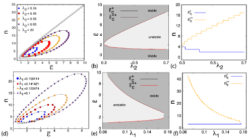
Figure 17: Linear stability of a homogeneous state in the continuum (phase-field) model of breakable chain coupled to an elastic background. Parametric study: (a,d) bifurcation points; (b,e) critical strains $\bar{\varepsilon}_{c}^{*}$ and $\bar{\varepsilon}_{c}^{**}$; (c,f) instability mode numbers $n_{c}^{*}$ and $n_{c}^{**}$. In (a-c) $\lambda_{1}=0.158114$ and in (d-f) $\lambda_{2}=0.34$.

In terms of the effective elastic energy density $f^{0}(\varepsilon)$ the bifurcation condition for $\bar{\varepsilon}_{c}$ reads

$$\left[\frac{\lambda_{1}^{2}}{\lambda_{2}^{2}}\frac{f^{0}(\bar{\varepsilon}_{c})}{\bar{\varepsilon}_{c}^{2}}+\frac{\partial^{2}f^{0}}{\partial\varepsilon^{2}}(\bar{\varepsilon}_{c})\right]^{2}-\frac{\lambda_{1}^{2}}{\lambda_{2}^{2}}\frac{1}{\bar{\varepsilon}_{c}^{2}}\left[\frac{1}{\bar{\varepsilon}_{c}}\frac{\partial f^{0}}{\partial\varepsilon}(\bar{\varepsilon}_{c})-\frac{\partial^{2}f^{0}}{\partial\varepsilon^{2}}(\bar{\varepsilon}_{c})\right]=0.$$ (27)

Then the critical mode number $n_{c}$ is

$$(n_{c}\pi)^{2}=-\frac{(\frac{\lambda_{1}}{\lambda_{2}})^{2}\frac{f^{0}(\bar{\varepsilon}_{c})}{\bar{\varepsilon}_{c}^{2}}+\frac{\partial^{2}f^{0}}{\partial\varepsilon^{2}}(\bar{\varepsilon}_{c})}{\frac{\lambda_{1}^{2}}{2\bar{\varepsilon}_{c}^{2}}\left[\frac{1}{\bar{\varepsilon}_{c}}\frac{\partial f^{0}}{\partial\varepsilon}(\bar{\varepsilon}_{c})-\frac{\partial^{2}f^{0}}{\partial\varepsilon^{2}}(\bar{\varepsilon}_{c})\right]}.$$ (28)

The parametric dependence of the solutions of (26), is illustrated in Fig. 17(a,d). We see the return of the closed loops as in the case of a pantograph-reinforced chain, see Fig. 9(a,d). The loops becomes larger as $\lambda_{2}\rightarrow\infty$, and in the limit, we recover the loopless case of classical brittle fracture, see Fig. 14(a). Such ‘opening’ of the stability boundaries is reminiscent of the theory of wrinkles in stretched elastic sheets as one moves from the fully nonlinear 3D theory for, say neo-Hookean material, to a simplified Foppl-von Karman theory [59].

In Fig. 17(b,e), we show the parametric dependence of the critical strain, see (27). Due to the presence of an elastic background, the re-entry behavior of the affine configuration is recovered with the emergence of the two critical strains $\bar{\varepsilon}_{c}^{*}$ and $\bar{\varepsilon}_{c}^{**}$ representing, respectively, the lower and upper limits of stability for the homogeneous state, see Fig. 17 (b,e). The parametric dependence of the critical wavenumber $n_{c}$, shown in Fig. 17(c,f), departs from what we have seen in the model of pantograph-reinforced chain on an elastic foundation as the critical wavenumber $n_{c}(\bar{\varepsilon}_{c}^{*})$ is now different from the critical wavenumber $n_{c}(\bar{\varepsilon}_{c}^{**})$. We can link this result with the fact that the re-stabilization (or healing) of the affine state at large levels of stretching is enforced by a different physical mechanism in our two settings: the bending induced ‘weak’ nonlocality of ‘ferromagnetic’ type in the case of the pantograph-reinforced breakable chain, and the elastic foundation-induced ‘strong’ nonlocality of anti-ferromagnetic type in the case of the chain coupled to an elastic foundation.

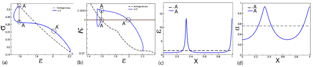
Figure 18: First instability along the LEM path in the continuum model of a breakable chain coupled to an elastic background: (a) macroscopic strain-stress response showing the discontinuous transition A’$\rightarrow$A from affine to non-affine states at the critical strain $\bar{\varepsilon}_{c}^{*}$; (b) smallest eigenvalue of the second variation for the branch with $n=0$ and $n=3$ as a function of the loading parameter $\bar{\varepsilon}$; (c,d) strain and damage parameter profiles before and after the A’$\rightarrow$A transition. Parameters: $\lambda_{1}=0.158114$, $\lambda_{2}=0.34$.

Consider now the post-bifurcational response under the LEM protocol.

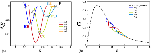
Figure 19: Mechanical response in the continuum (phase-field) model of a breakable chain on elastic foundation deformed according to the GEM protocol: (a) the energy difference between the affine and non-affine configurations, letters G,B,C,D,E,F indicate dissipation-free branch switching events; (b) the corresponding macroscopic strain-stress relations. Parameters: $\lambda_{1}=0.158114$, $\lambda_{2}=0.34$.

The stress-strain response, following the first instability at the point A’, is illustrated in Fig. 18(a) for a particular choice of parameters $\lambda_{1}$ and $\lambda_{2}$. The branch switching transition A’$\rightarrow$A brings the system from the trivial branch with $n=0$ to the nontrivial equilibrium branch with $n=3$, and the linear stability of the ensuing non-affine configuration is illustrated in Fig. 18(b) where we show that in point A the smallest eigenvalue of the corresponding second variation is positive. In Fig. 18(c,d) we show that during this symmetry breaking transition two localized cracks nucleate simultaneously: one inside the domain and one on the boundary. Due to the subcritical nature of the bifurcation, the dissipative transition A’$\rightarrow$A is accompanied by an abrupt stress drop, see Fig. 18(a).

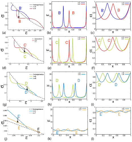
Figure 20: Zoom in on various dissipation-free GEM transitions depicted in Fig. 19: (a,d,g,j) stress-strain relations, (b,e,h,k) strain profiles, (c,f,i,l) damage parameter profiles. Parameters: $\lambda_{1}=0.158114$, $\lambda_{2}=0.34$.

As we see from Fig. 18(b), the equilibrium configurations with $n=3$ loses linear stability at the point A”. To describe the subsequent transformations, we need to reconstruct the global picture and consider equilibrium configurations with different values of $n$. The corresponding solutions of the nonlinear system (25) are shown in Fig. 19 where we collected information about the equilibrium branches with $n=3,...,7$.

We observe that under the LEM protocol, the only available transition from point A” is to the branch with $n=4$, which is locally stable in the corresponding range of applied strains $\bar{\varepsilon}$. Beyond this point, a sequence of dissipative LEM transitions takes place with more and more cracks appearing sequentially, till finally, at a sufficiently large value of the loading parameter, the strain localization abruptly disappears, and the damage becomes uniformly distributed. The detailed picture of the LEM response will be laid out elsewhere, while below, for a difference, we summarize the system’s behavior along the GEM dynamic path.

The access to the equilibrium branches shown in Fig. 19 allow one to describe all the successive branch switching events in the process of quasi-static stretching. The nature of the corresponding transitions is illustrated in Fig. 20 which should be compared with the analogous Fig. 12 and Fig. 13 showing the succession of the GEM transitions in the system reinforced by pantograph substructure.

We observe in Fig. 19 that along the GEM path the first non-symmetric, two-crack configuration nucleates non-dissipatively at the point G’. The corresponding transition G’$\rightarrow$G marks the switch form the branch $n=0$ to the branch $n=3$, see Fig. 19(a). The next GEM transition at point B’ to the branch $n=4$ takes place before the corresponding linear instability limit, marked by the point A” is reached, see Fig. 19(a). The configuration which emerges as a result of the non-dissipative transition B’$\rightarrow$B is illustrated in Fig. 20 (a-c). As we see, the non-symmetric two-crack configuration transforms into the symmetric three-crack configuration with one localized crack in the center and two localized cracks around the boundaries. The next GEM transition C’$\rightarrow$C breaks the symmetry again, creating a three-crack configuration with two localized cracks inside and one localized crack on the boundary. Then, the symmetry is recovered during the transition D’$\rightarrow$D when the four-crack configuration emerges with two localized cracks inside and two localized cracks around the boundaries. Finally, after yet another symmetry breaking transition E’$\rightarrow$E the affine configuration is retrieved at the point F.

Note that with each successive GEM transition, both the strain $\varepsilon(x)$ and the measure of damage $\alpha(x)$ become less localized. In particular, just before the affine state is recovered, that sample appears almost unstressed with slight modulation of strain but with the level of damage almost uniformly high. In such configuration, which absorbs all the work of the loading device, the elastic strain is systematically replaced by the inelastic strain. Instead, along the corresponding LEM path, the energy is dissipated instead of being accumulated.

Note also that in the phase-field model, even in the presence of an elastic background, cracks remain localized almost all the way till they disappear in the state entirely dominated by the elastic background. Their number increases with stretch, however, in contrast to the model of pantograph-reinforced chain, the extended domains of distributed damage do not appear. In this sense, the reinforcement through the elastic foundation is not equivalent to the reinforcement through the bending dominated sub-structure. Therefore, the floppy substructure is indeed the crucial element of the proposed metamaterial design.

6 Conclusions

While some natural materials break with the formation of a single macro-crack, other natural materials exhibit multiple, almost diffuse macro-cracking. The difference between the two classes of material behavior is reflected in the nomenclature of fracture and damage mechanics. The two are often presented as separate disciplines addressing fundamentally distinct failure modes; a closely related antithesis is between brittle and quasi-brittle (ductile) responses.

Various attempts have been made to explain the difference between these two failure mechanisms by linking them, for instance, to preexisting defects [91, 18] or to the convexity properties of the cohesive energy [13, 92]. Under the assumption that "to understand, is to build", we posed in this paper the problem of designing an artificially engineered metamaterial that can be potentially switched from one of these failure modes to another.

Our main idea is that the range of stress redistribution, exemplified by the effective rigidity, may serve as the factor affecting, at least in some cases, the localization properties of fracture phenomenon [24]. In particular, we conjectured that the transition from ‘stretching dominated’ to ‘bending dominated’ elasticity [29, 25, 93] will favor strain delocalization and will be able to change the character of the cracking process from brittle-like to ductile-like.

To check this possibility, we followed various earlier insights and proposed the simplest conceptual design of a high-toughness, pseudo-ductile metamaterial with nominally brittle sub-elements. Using this toy example we showed that by affecting the nature of the structural connectivity inside an elastic system, one can transform a brittle structure, which fails with the formation of highly localized cracks, into an apparently ductile structure exhibiting de-localized damage. The desired nominal ductility is achieved by elastic coupling of a conventional stretching-dominated brittle sub-structure with another floppy sub-structure that can transmit bending-dominated nonlocal elastic interactions.

To substantiate these conclusions, we solved a series of elementary 1D model problems showing how the presence of a floppy sub-structure can suppress strain localization and induce the formation of diffuse zones of microcracking. To facilitate the analysis we developed an asymptotically equivalent continuum theory of Ginzburg-Landau type with strain as the order parameter. Since the local part of the corresponding energy is represented by a single-well potential with sub-linear growth, the nonlocal (gradient) term becomes relevant ‘volumetrically’ even though there is a small coefficient in front of it. This is unusual, given that in the conventional theory of phase transitions, a similar term is only relevant for the description of narrow transition zones. We showed that in tensile loading, the proposed Ginzburg-Landau elastic model reproduces the behavior of the original discrete model adequately, including the intriguing re-entrant isola-center bifurcation. The main lesson is that the re-stabilization of the affine response can be accomplished by bending rather than stretching elasticity.

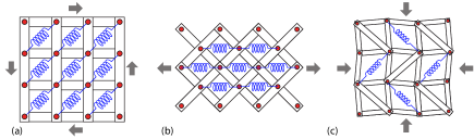
Figure 21: Three examples of the 2D spring systems reinforced by floppy substructures with bending dominated elasticity that can be expected to exhibit fracture de-localization under: (a) shear, (b) uni-axial tension, (c) bi-axial (hydrostatic) compression.

The analysis of the same system coupled to an elastic background revealed a complex succession of fracture patterns. Depending on the presence or absence of the floppy reinforcing substructure, the emerging microstructures include either diffuse zones of microcracking or isolated macrocracks. Our ability to manipulate such patterns in specially designed metamaterials can mimic living cells’ ability to assemble and dis-assemble various load-carrying ‘frames’ that are fine-tuned to match the particular types of loading. The presence in the space of the loading parameters of a finite range where the mechanical response of the system is non-affine may be of interest to industrial applications. For instance, it implies that under monotone driving, the appropriately designed metamaterial can produce a transient, information-carrying failure pattern that first comes out but then gets erased.

The proposed prototypical design of the pantograph-reinforced mass-spring chain serves only as a proof of concept, and the technologically relevant 3D brittle metamaterials, reinforced by bending-dominated floppy networks, would still have to be designed and fabricated. This task, however, is not unrealistic, given the already existing 3D printing capabilities which open access to high-contrast composite networks with inextensible but bendable elements. Three potentially interesting 2D designs of this type, involving floppy substructures with bending dominated elasticity, and expected to show fracture delocalization in either shear, uni-axial tension or bi-axial (hydrostatic) compression, are shown in Fig. 21. They demonstrate how the harnessed floppiness can be used to achieve high toughness in low-weight structures.

Future work in the proposed direction must also include the account of the irreversibility of damage which was downplayed in our analysis. Finite size effects were also largely neglected. Interesting problems will be raised by the development of rigorous finite strain continuum approximations in higher dimensions accounting for both ‘local’ and ‘nonlocal’ sub-structures. The associated continuum problems are of higher-order, requiring the development of new analytical and numerical approaches.

7 Acknowledgments

The authors are grateful to G. Vitale for his various contributions to the initial version of this paper. O. U. S. acknowledges helpful discussions with I. R. Ioanescu. O. U. S. was supported by the grants ANR-19-CE08-0010-01, ANR-20-CE91-0010, and L. T. by the grant ANR-10-IDEX-0001-02 PSL.

References

- Bertram Broberg [1999] Bertram Broberg K. Cracks and Fracture. Elsevier; 1999.
- Hans J. Herrmann and Roux [1990] Hans J. Herrmann E, Roux S. Statistical Models for the Fracture of Disordered Media. Elsevier; 1990.
- Kanninen and Popelar [1985] Kanninen MF, Popelar CL. Advanced fracture mechanics. Oxford University Press; 1985.
- Truskinovsky [1996] Truskinovsky L. Fracture as a phase transition. In: Batra R, M.F. B, editors. Contemporary research in the mechanics and mathematics of materials. CIMNE, Barcelona; 1996, p. 322–32.
- Triantafyllidis and Aifantis [1986] Triantafyllidis N, Aifantis E. A gradient approach to localization of deformation. i. hyperelastic materials. Journal of Elasticity 1986;16(3):225–37.
- Belytschko et al. [2003] Belytschko T, Chen H, Xu J, Zi G. Dynamic crack propagation based on loss of hyperbolicity and a new discontinuous enrichment. Int J Numer Meth Engng 2003;58(12):1873–905.
- Baker and Munroe [1988] Baker I, Munroe PR. Improving intermetallic ductility and toughness. Journal of Metals 1988;40(2):28–31.
- Swadener et al. [2002] Swadener JG, Baskes MI, Nastasi M. Molecular dynamics simulation of brittle fracture in silicon. Phys Rev Lett 2002;89(8):085503.
- Evans and Faber [1981] Evans AG, Faber KT. Toughening of ceramics by circumferential microcracking. J Am Ceram Soc 1981;64(7):394–8.
- Faber et al. [1988] Faber KT, Iwagoshi T, Ghosh A. Toughening by stress-induced microcracking in two-phase ceramics. J Am Ceram Soc 1988;71(9):C–399.
- Budiansky et al. [1983] Budiansky B, Hutchinson JW, Lambropoulos JC. Continuum theory of dilatant transformation toughening in ceramics. Int J Solids Struct 1983;19(4):337–55.
- Green [2018] Green DJ. Transformation Toughening Of Ceramics. 1st edition ed.; CRC Press; 2018.
- Del Piero and Truskinovsky [2001] Del Piero G, Truskinovsky L. Macro- and micro-cracking in one-dimensional elasticity. Int J Solids Struct 2001;38(6):1135–48.
- Cherkaev and Slepyan [1995] Cherkaev A, Slepyan L. Waiting element structures and stability under extension. Int J Damage Mech 1995;4(1):58–82.
- Wiederhorn [1984] Wiederhorn SM. Brittle fracture and toughening mechanisms in ceramics. Annu Rev Mater Sci 1984;14(1):373–403.
- Davies and Ogwu [1995] Davies TJ, Ogwu AA. A possible route to improving the ductility of brittle intermetallic compounds. J Alloys Compd 1995;228(1):105–11.
- Yang et al. [2018] Yang T, Zhao YL, Liu WH, Zhu JH, Kai JJ, Liu CT. Ductilizing brittle high-entropy alloys via tailoring valence electron concentrations of precipitates by controlled elemental partitioning. Materials Research Letters 2018;6(10):600–6.
- Borja da Rocha and Truskinovsky [2020] Borja da Rocha H, Truskinovsky L. Rigidity-Controlled crossover: From spinodal to critical failure. Phys Rev Lett 2020;124(1):015501.
- Daniel et al. [2017] Daniel R, Meindlhumer M, Baumegger W, Zalesak J, Sartory B, Burghammer M, et al. Grain boundary design of thin films: Using tilted brittle interfaces for multiple crack deflection toughening. Acta Mater 2017;122:130–7.
- Ebrahimi et al. [2019] Ebrahimi MT, Balint DS, Sutton AP, Dini D. A discrete crack dynamics model of toughening in brittle polycrystalline material by crack deflection. Eng Fract Mech 2019;214:95–111.
- Wu and Fan [2020] Wu H, Fan G. An overview of tailoring strain delocalization for strength-ductility synergy. Prog Mater Sci 2020;113:100675.
- Liang et al. [2020] Liang F, Zhang B, Yong Y, Luo XM, Zhang GP. Enhanced strain delocalization through formation of dispersive micro shear bands in laminated ni. Int J Plast 2020;132:102745.
- Radi et al. [2020] Radi K, Jauffres D, Deville S, Martin CL. Strength and toughness trade-off optimization of nacre-like ceramic composites. Composites Part B 2020;183:107699.
- Driscoll et al. [2016] Driscoll MM, Chen BGG, Beuman TH, Ulrich S, Nagel SR, Vitelli V. The role of rigidity in controlling material failure. Proc Natl Acad Sci 2016;113(39):10813–7.
- Buxton and Clarke [2007] Buxton GA, Clarke N. “bending to stretching” transition in disordered networks. Phys Rev Lett 2007;98(23)(238103).
- Broedersz and MacKintosh [2014] Broedersz CP, MacKintosh FC. Modeling semiflexible polymer networks. Rev Mod Phys 2014;86:995–1036.
- Zadpoor [2016] Zadpoor AA. Mechanical meta-materials. Materials Horizons 2016;3(5):371–81.
- Alibert et al. [2003a] Alibert JJ, Seppecher P, Dell’Isola F. Truss Modular Beams with Deformation Energy Depending on Higher Displacement Gradients. Mathematics and Mechanics of Solids 2003a;8:51–73.
- van der Giessen [2011] van der Giessen E. Materials physics: Bending maxwell’s rule. Nat Phys 2011;7(12):923–4.
- Franciosi et al. [2019] Franciosi P, Spagnuolo M, Salman OU. Mean green operators of deformable fiber networks embedded in a compliant matrix and property estimates. Continuum Mech Thermodyn 2019;31(1):101–32.
- Maxwell [1864] Maxwell JC. L. on the calculation of the equilibrium and stiffness of frames. The London, Edinburgh, and Dublin Philosophical Magazine and Journal of Science 1864;27(182):294–9.
- Calladine [1978] Calladine CR. Buckminster fuller’s “tensegrity” structures and clerk maxwell’s rules for the construction of stiff frames. Int J Solids Struct 1978;14(2):161–72.
- Schenk and Guest [2014] Schenk M, Guest SD. On zero stiffness. Proc Inst Mech Eng Part C 2014;228(10):1701–14.
- Pideri and Seppecher [1997] Pideri C, Seppecher P. A second gradient material resulting from the homogenization of an heterogeneous linear elastic medium. Continuum Mechanics and Thermodynamics 1997;9(5).
- Cherednichenko et al. [2006] Cherednichenko KD, Smyshlyaev VP, Zhikov VV. Non-local homogenized limits for composite media with highly anisotropic periodic fibres. Proceedings of the Royal Society of Edinburgh: Section A Mathematics 2006;136(01).
- Camar-Eddine and Seppecher [2003] Camar-Eddine M, Seppecher P. Determination of the closure of the set of elasticity functionals. Arch Ration Mech Anal 2003;170(3):211–45.
- Boutin et al. [2013] Boutin C, Soubestre J, Dietz MS, Taylor C. Experimental evidence of the high-gradient behaviour of fiber reinforced materials. European Journal of Mechanics-A/Solids 2013;42.
- Bacca et al. [2013] Bacca M, Bigoni D, Dal Corso F, Veber D. Mindlin second-gradient elastic properties from dilute two-phase cauchy-elastic composites. part i: Closed form expression for the effective higher-order constitutive tensor. Int J Solids Struct 2013;50(24):4010–9.
- Truskinovsky and Zanzotto [1996] Truskinovsky L, Zanzotto G. Ericksen’s bar revisited : Energy wiggles. J Mech Phys Solids 1996;44(8):1371–408.
- Golubović and Lubensky [1989] Golubović L, Lubensky TC. Nonlinear elasticity of amorphous solids. Phys Rev Lett 1989;63(10)(1082).
- Marconi and Jagla [2005] Marconi VI, Jagla EA. Diffuse interface approach to brittle fracture. Phys Rev E 2005;71:036110.
- Triantafyllidis and Bardenhagen [1993] Triantafyllidis N, Bardenhagen S. On higher order gradient continuum theories in 1-d nonlinear elasticity. derivation from and comparison to the corresponding discrete models. Journal of Elasticity 1993;33(3):259–93.
- Placidi [2015] Placidi L. A variational approach for a nonlinear 1-dimensional second gradient continuum damage model. Continuum Mech Thermodyn 2015;27:623–38.
- Le et al. [2018] Le DT, Marigo JJ, Maurini C, Vidoli S. Strain-gradient vs damage-gradient regularizations of softening damage models. Comput Methods Appl Mech Eng 2018;340:424–50.
- Fokoua et al. [2014a] Fokoua L, Conti S, Ortiz M. Optimal scaling in solids undergoing ductile fracture by void sheet formation. Arch Ration Mech Anal 2014a;212(1):331–57.
- Fokoua et al. [2014b] Fokoua L, Conti S, Ortiz M. Optimal scaling laws for ductile fracture derived from strain-gradient microplasticity. J Mech Phys Solids 2014b;62:295–311.
- Zhang et al. [2013] Zhang L, Lake SP, Barocas VH, Shephard MS, Picu RC. Cross-linked fiber network embedded in an elastic matrix. Soft Matter 2013;9:6398–405.
- Ren and Truskinovsky [2000a] Ren X, Truskinovsky L. Finite scale microstructures in nonlocal elasticity. Journal of elasticity and the physical science of solids 2000a;59(1-3):319–55.
- Barenblatt and Prostokishin [1993] Barenblatt GI, Prostokishin VM. A mathematical model of damage accumulation taking into account microstructural effects. Eur J Appl Math 1993;4(3):225–40.
- Frémond and Nedjar [1996] Frémond M, Nedjar B. Damage, gradient of damage and principle of virtual power. Int J Solids Struct 1996;33(8):1083–103.
- Bourdin et al. [2000] Bourdin B, Francfort GA, Marigo JJ. Numerical experiments in revisited brittle fracture. J Mech Phys Solids 2000;48(4):797–826.
- Lorentz and Andrieux [2003] Lorentz E, Andrieux S. Analysis of non-local models through energetic formulations. Int J Solids Struct 2003;40(12):2905–36.
- Benallal and Marigo [2006] Benallal A, Marigo JJ. Bifurcation and stability issues in gradient theories with softening. Modell Simul Mater Sci Eng 2006;15(1):S283.
- Ambrosio and Tortorelli [1990] Ambrosio L, Tortorelli VM. Approximation of functional depending on jumps by elliptic functional via t-convergence. Communications on Pure and Applied Mathematics 1990;43(8):999–1036.
- Aranson et al. [2000] Aranson IS, Kalatsky VA, Vinokur VM. Continuum field description of crack propagation. Phys Rev Lett 2000;85(1):118–21.
- Karma et al. [2001] Karma A, Kessler DA, Levine H. Phase-field model of mode iii dynamic fracture. Phys Rev Lett 2001;87:045501.
- Eastgate et al. [2002] Eastgate LO, Sethna JP, Rauscher M, Cretegny T, others . Fracture in mode I using a conserved phase-field model. Physical review E 2002;.
- Golubitsky and Schaeffer [1985] Golubitsky M, Schaeffer DG. A brief introduction to the central ideas of the theory. In: Golubitsky M, Schaeffer DG, editors. Singularities and Groups in Bifurcation Theory: Volume I. New York, NY: Springer New York; 1985, p. 1–50.
- Li and Healey [2016] Li Q, Healey TJ. Stability boundaries for wrinkling in highly stretched elastic sheets. J Mech Phys Solids 2016;97:260–74.
- Puglisi and Truskinovsky [2005] Puglisi G, Truskinovsky L. Thermodynamics of rate-independent plasticity. J Mech Phys Solids 2005;53(3):655–79.
- Bochkanov and Bystritsky [2013] Bochkanov S, Bystritsky V. Alglib. Available from: www alglib net 2013;.
- Chan and Keller [1982] Chan TFC, Keller HB. Arc-Length continuation and multigrid techniques for nonlinear elliptic eigenvalue problems. SIAM J Sci and Stat Comput 1982;3(2):173–94.
- Sanderson and Curtin [2016] Sanderson C, Curtin R. Armadillo: a template-based c++ library for linear algebra. J Open Source Softw 2016;1(2):26.
- Rosakis et al. [2021] Rosakis P, Healey TJ, Alyanak U. The inverse-deformation approach to fracture. J Mech Phys Solids 2021;150:104352.
- Alibert et al. [2003b] Alibert JJ, Seppecher P, Dell’Isola F. Truss modular beams with deformation energy depending on higher displacement gradients. Math Mech Solids 2003b;8(1):51–73.
- Charlotte and Truskinovsky [2002] Charlotte M, Truskinovsky L. Linear elastic chain with a hyper-pre-stress. J Mech Phys Solids 2002;50(2):217–51.
- Curtin et al. [1998] Curtin WA, Ahn BK, Takeda N. Modeling brittle and tough stress–strain behavior in unidirectional ceramic matrix composites. Acta Mater 1998;46(10):3409–20.
- Truskinovsky [2010] Truskinovsky L. Fracture as a phase transition, in “contemporary research in the mechanics and mathematics of materials,” CIMNE, barcelona,(1996), 322–332. Received August 2010;.
- Braides et al. [1999] Braides A, Maso GD, Garroni A. Variational formulation of softening phenomena in fracture mechanics: The One-Dimensional case. Arch Ration Mech Anal 1999;146(1):23–58.
- Braides and Truskinovsky [2008] Braides A, Truskinovsky L. Asymptotic expansions by -convergence. Continuum Mech Thermodyn 2008;20(1):21–62.
- Blanc et al. [2002] Blanc X, Le Bris C, Lions PL. From molecular models to continuum mechanics. Arch Ration Mech Anal 2002;164(4):341–81.
- Charlotte and Truskinovsky [2008] Charlotte M, Truskinovsky L. Towards multi-scale continuum elasticity theory. Continuum Mech Thermodyn 2008;20(3):133–61.
- Lifshits and Rybnikov [1985] Lifshits AE, Rybnikov GL. Dissipative structures and couette flow of a non-newtonian fluid. In: Doklady Akademii Nauk; vol. 281. 1985, p. 1088–93.
- Lifshitz and Rybnikov [1985] Lifshitz AE, Rybnikov GL. Dissipative structures and couette flow in a non-newtonian fluid. Soviet Physics Doklady 1985;20:275.
- Dellwo et al. [1982] Dellwo D, Keller HB, Matkowsky BJ, Reiss EL. On the birth of isolas. SIAM Journal on Applied Mathematics 1982;42(5).
- Healey et al. [2013] Healey TJ, Li Q, Cheng RB. Wrinkling behavior of highly stretched rectangular elastic films via parametric global bifurcation. J Nonlinear Sci 2013;23(5):777–805.
- Truskinovsky and Zanzotto [1995] Truskinovsky L, Zanzotto G. Finite-scale microstructures and metastability in one-dimensional elasticity. Meccanica 1995;30(5):577–89.
- Novick-Cohen and Segel [1984] Novick-Cohen A, Segel LA. Nonlinear aspects of the Cahn-Hilliard equation. Physica D 1984;10(3):277–98.
- Doedel et al. [2008] Doedel EJ, Champneys AR, Dercole F, Fairgrieve T, Kuznetsov Y, Oldeman B, et al. AUTO-07P: Continuation and Bifurcation Software for Ordinary Differential Equations; 2008.
- Liu and Quek [2013] Liu GR, Quek SS. The Finite Element Method: A Practical Course. Butterworth-Heinemann; 2013.
- Grimstad et al. [2015] Grimstad B, et al. SPLINTER: a library for multivariate function approximation with splines. http://github.com/bgrimstad/splinter; 2015.
- van Doorn et al. [2017] van Doorn JM, Lageschaar L, Sprakel J, van der Gucht J. Criticality and mechanical enhancement in composite fiber networks. Phys Rev E 2017;95(4-1):042503.
- Cortes and Elliott [2012] Cortes DH, Elliott DM. Extra-fibrillar matrix mechanics of annulus fibrosus in tension and compression. Biomech Model Mechanobiol 2012;11(6):781–90.
- Lynch et al. [2017] Lynch B, Bancelin S, Bonod-Bidaud C, Gueusquin JB, Ruggiero F, Schanne-Klein MC, et al. A novel microstructural interpretation for the biomechanics of mouse skin derived from multiscale characterization. Acta Biomater 2017;50:302–11.
- Vainchtein et al. [1999] Vainchtein A, Healey TJ, Rosakis P. Bifurcation and metastability in a new one-dimensional model for martensitic phase transitions. Computer Methods in Applied Mechanics and Engineering 1999;170(3–4):407 –21.
- Ren and Truskinovsky [2000b] Ren X, Truskinovsky L. Finite scale microstructures in nonlocal elasticity. Journal of Elasticity 2000b;59(1-3):319–55.
- Belintsev et al. [1981] Belintsev BN, Livshits MA, Volkenstein MV. Pattern formation in systems with nonlocal interactions. Z Phys B: Condens Matter 1981;44(4):345–51.
- Toko and Yamafuji [1990] Toko K, Yamafuji K. Bifurcation characteristics and spatial patterns in an integro-differential equation. Physica D 1990;44(3):459–70.
- Pham et al. [2011] Pham K, Marigo JJ, Maurini C. The issues of the uniqueness and the stability of the homogeneous response in uniaxial tests with gradient damage models. J Mech Phys Solids 2011;59(6):1163 –90.
- Pellegrini et al. [2010] Pellegrini YP, Denoual C, Truskinovsky L. Phase-field modeling of nonlinear material behavior. In: Hackl K, editor. IUTAM Symposium on Variational Concepts with Applications to the Mechanics of Materials; vol. 21 of IUTAM Bookseries. Springer Netherlands; 2010, p. 209–20.
- Shekhawat et al. [2013] Shekhawat A, Zapperi S, Sethna JP. From damage percolation to crack nucleation through finite size criticality. Phys Rev Lett 2013;110(18):185505.
- Rinaldi [2013] Rinaldi A. Bottom-up modeling of damage in heterogeneous quasi-brittle solids. Continuum Mech Thermodyn 2013;25(2-4):359–73.
- Salman et al. [2019] Salman OU, Vitale G, Truskinovsky L. Continuum theory of bending-to-stretching transition. Phys Rev E 2019;100(5-1):051001.