A Lower Bound for Dynamic Fractional Cascading
Abstract
We investigate the limits of one of the fundamental ideas in data structures: fractional cascading. This is an important data structure technique to speed up repeated searches for the same key in multiple lists and it has numerous applications. Specifically, the input is a “catalog” graph, , of constant degree together with a list of values assigned to every vertex of . The goal is to preprocess the input such that given a connected subgraph of and a single query value , one can find the predecessor of in every list that belongs to . The classical result by Chazelle and Guibas shows that in a pointer machine, this can be done in the optimal time of where is the total number of values. However, if insertion and deletion of values are allowed, then the query time slows down to . If only insertions (or deletions) are allowed, then once again, an optimal query time can be obtained but by using amortization at update time.
We prove a lower bound of on the worst-case query time of dynamic fractional cascading, when queries are paths of length . The lower bound applies both to fully dynamic data structures with amortized polylogarithmic update time and incremental data structures with polylogarithmic worst-case update time. As a side, this also proves that amortization is crucial for obtaining an optimal incremental data structure.
This is the first non-trivial pointer machine lower bound for a dynamic data structure that breaks the barrier. In order to obtain this result, we develop a number of new ideas and techniques that hopefully can be useful to obtain additional dynamic lower bounds in the pointer machine model.
1 Introduction
Our motivation lies at the intersection of two important topics: the fractional cascading problem and proving dynamic lower bounds in the pointer machine model. We delve into each of them below but to summarize, we give the first lower bound for the fractional cascading problem, which we believe is the first major progress on this problem since 1988, and in addition, our lower bound is the first non-trivial pointer machine lower bound for a dynamic data structure that breaks the barrier.
By now fractional cascading is one of the fundamental and classical techniques in data structures and in fact, it is routinely taught in various advanced data structures courses around the world. Its importance is due to a very satisfying and elegant answer that it gives to a common problem in data structures: how to search for the same key in many different lists? Fractional cascading provides a very general framework to solve the problem: the input can be any graph of constant degree, , called the “catalog” graph. Also as part of the input, each vertex of is associated with a “catalog” that is simply a list of values from an ordered set. The goal is to build a data structure such that given a query value from the ordered set, and a connected subgraph of , one can find the predecessor of in every catalog associated with the vertices of . As the lists of different vertices are unrelated, at the first glance it seems difficult to do anything other than just a binary search in each list, for a total query time of . Fractional cascading reduces this time to , equivalent to constant time per predecessor search, after investing an initial time.
This problem of performing iterative searches has shown up multiple times in the past. For example, in 1982 Vaishnai and Wood [28] used “layered segment tree” to break-through this barrier and in 1985 research on the planar version of orthogonal range reporting led Willard [29] to the notion of “downpointers” that allowed him to do searches in time. The next year and in a two-part work, Chazelle and Guibas presented the fully-fledged framework of fractional cascading and used it to attack a number of very important problems in data structures [13, 14]: they presented a linear-size data structure that could answer fractional cascading queries in time. As discussed, this is optimal in the comparison model but also in the pointer machine model. The idea behind fractional cascading also shows up in other areas, e.g., some of the important milestones in parallel algorithms were made possible by similar ideas (e.g., Cole’s seminal time parallel sorting algorithm [18]; see also [9] for further applications in the PRAM model).
The dynamic case.
However, despite its importance, the dynamic version of the problem is still open. Chazelle and Guibas themselves investigated this variant. Here, some optimal results were obtained quickly: If only insertions (or deletions) are allowed, then updates can be done in amortized time (i.e., in time over a sequence of updates) while keeping the optimal query time. However, if both insertions and deletions are allowed then the query time becomes . After presenting the dynamic case, Chazelle and Guibas expressed dissatisfaction at their solution, wondering whether it is optimal 111They write [13]: “The most unsatisfactory aspect of our treatment of fractional cascading is the handling of the dynamic situation. Is our method optimal?.”. Later work by Mehlhorn and Näher [23] improved this dynamic solution by cutting down update time to amortized time but they could not offer any improvement on the query time. Dietz and Raman removed the amortization to make the update time of worst-case [19]. Finally, while working on the dynamic vertical ray shooting problem, Giora and Kaplan [20] showed that the extra factor is in fact an additive term when considering the degree of the graph , i.e., queries can be performed in time where is the maximum degree of . However, despite all this attention given to the dynamic version of the problem, the extra factor behind the output size persisted.
The results by Chazelle and Guibas hold in the general pointer machine model: the memory of the data structure is composed of cells where each cell can store one element as well as two pointers to other memory cells and the only way to access a memory cell is to follow a pointer that points to the memory cell. In this model, it seems difficult to improve or remove the extra factor. On the other hand, lower bound techniques for dynamic data structure problems in the pointer machine model are quite under-developed. We will discuss these next.
The pointer machine lower bounds.
As it will be evidence soon, proving dynamic lower bounds in this model is very challenging, even though it is one of the classical models of computation and it is a very popular model to represent tree-based data structures as well as many data structures in computational geometry. Here, our focus will be on the lower bound results only.
Many fundamental algorithmic and data structure problems were studied in 1970s and in the pointer machine model. Perhaps the most celebrated lower bound result of this period is Tarjan’s lower bound for the complexity of “union” operations and “find” operations when , [27]. This was later improved to [10, 25] for any and . Here is the inverse Ackermann function. However, originally, the existing lower bounds needed a certain “separation assumption” that essentially disallowed placing pointers between some elements (e.g., elements from different sets) [27, 26, 10]. In 1988, Mehlhorn et al. [22] studied the dynamic predecessor search problem in the pointer machine model, under the name of “union-split-find” problem, and they proved that for large enough , a sequence of insertions, queries and deletions, requires time. This was a significant contribution since not only they proved this without using the separation assumption but also in the same paper they showed that the separation assumption can in fact result in loss of efficiency, i.e., a pointer machine without the separation assumption can outperform a pointer machine with the separation assumption. Following this and in 1996, La Poutre showed that lower bounds for the union-find problem still hold without the separation assumption [25]. We note that the lower bound of Mehlhorn et al. was later strengthened by Mulzer [24].
The lower bound of Mehlhorn et al. [22] on the dynamic predecessor search problem can be viewed as a “budge fractional cascading lower bound”. However, it only provides a very limited lower bound; essentially, it only applies to data structures that treat a dynamic fractional cascading query on a subgraph as a set of independent dynamic predecessor queries. But obviously, the data structure may opt to do something different and in fact in some cases something different is actually possible. For example, if is a path, then the dynamic fractional problem on reduces to the dynamic interval stabbing problem for which data structures with query time exist (e.g., using the classical segment tree data structure). As a result, the lower bound of Mehlhorn et al. [22] is not enough to rule out “clever” solutions that somehow circumvent treating the problem as a union of independent predecessor queries.
As far as we know, these are the major works on dynamic lower bounds in the pointer machine model. It turns out, proving non-trivial lower bounds in this model is in fact quite challenging. In all the dynamic lower bounds above, after being given a query, the data structure has time to answer it: in the dynamic predecessor problem studied by Mehlhorn et al. [22], the query is a pointer to an element and the data structure is to find the predecessor of in time. In the union-find problems, the query is once again a pointer to an element of a set, and the data structure should find the “label” of the element with very few pointer navigations. Contrast this with the fractional cascading problem: the query could be a subgraph of size , which would give the data structure at least time.
Lack of techniques for proving high pointer machine lower bounds for dynamic data structure is quite disappointing, specially compared to the static world where there are a lot of lower bounds to cite and at least two relatively easy-to-use lower bound frameworks. In fact, static pointer machine lower bounds are so versatile that they have been adopted to work in other models of computation, such as the I/O model. But not much has happened for a long time in the dynamic front.
1.1 Our Results.
We believe we have made significant progress in two fronts: we prove a lower bound of on the worst-case query time of dynamic fractional cascading, when queries are paths of length . Our lower bound actually is applicable in two scenarios: (i) when the data structure is fully dynamic and the update time is amortized and polylogarithmic (i.e., it takes time to perform any sequence of insertions or deletions) or (ii) in the incremental case, when the data structure is only required to do insertions but the update time must be polylogarithmic and worst-case. This proves that in an incremental data structure, amortization is required to keep the query time optimal, inline with the upper bounds [13].
As far as we are aware, this is the first non-trivial222 By “non-trivial” we mean a query lower bound that is asymptotically higher than the best lower bounds for the static version of the problem; clearly, any lower bound that one can prove for a static data structure problem, trivially applies to the dynamic case as well. pointer machine lower bound for a dynamic data structure that exceeds bound. Thus, we believe our technical contributions are also important. We introduce a number of ideas that up to our knowledge are new in this area. Unfortunately, our proof is quite technical and involves making a lot of definitions and small observations. Simplifying our techniques and turning them into a more easily applicable framework is an interesting open problem.
Finally, we remark that since we obtain our lower bound using a geometric construction, our results have another consequence: we can show that the dynamic rectangle stabbing problem in the pointer machine model requires query time, assuming polylogarithmic update time. The static problem can be solved in linear space and with query time [11] and thus our lower bound is the first provable separation result between dynamic vs static versions of a range range reporting problem.
2 The Model of Computation and Known Static Results
2.1 The Lower Bound Model.
We now formally introduce the particular variant of the pointer machine model that is used for proving lower bounds. Here, the memory is composed of cells and each cell can store one value from the catalogue of any vertex of . In addition, each cell can store up to two pointers to other memory cells. We think of the memory of the data structure as a directed graph with out-degree at most two where a pointer from a memory cell to a memory cell is represented as a directed edge from to . There is a special cell, the root, that the data structure can always access for free.
We place two restrictions in front of the data structure: one, the only way to access a memory cell is first to access a memory cell that points to and then to use the pointer from to to access . And two, the input values must be stored atomically by the data structure and the only way the data structure can output any input value is to access a memory cell that stores .
On the other hand, we only charge for two operations: At the query time, we only charge for pointer navigations, i.e., only count how many cells the data structure accesses. At the update time, we only count the number of cells that the data structure changes.
Thus, in effect we grant the data structure infinite computational power, as well as full information regarding the structure of the memory graph; e.g., the query algorithm fully knows where each input value is stored and it can compute the best possible way (i.e., solve an implicit Steiner subgraph problem) to reach a cell that stores a desired output value or the update algorithm can figure out how to change the minimum number of pointers to allow the query algorithm the best possible ability to do the navigation. In essence, a dynamic lower bound is a statement about “the connectivity bottleneck” of a dynamic directed graph with out-degree two.
2.2 Static Lower Bounds.
Lower bounds for static data structure problems in the pointer machine model have a very good “success rate”, meaning, there are many problems for which these lower bounds match or almost match the best known upper bounds. We can attribute the initiation of this line of research to Bernard Chazelle, who in 1990 [12] introduced the first framework for proving lower bounds for static data structures in the pointer machine model and also used it to prove an optimal space lower bound for the important orthogonal range reporting problem. Since then, for other important problems, similar lower bounds have been found: optimal and almost optimal space-time trade-offs for the fundamental simplex range reporting problem [1, 16], optimal query lower bounds for variants of “two-dimensional fractional cascading” [15, 4], optimal query lower bounds for the axis-aligned rectangle stabbing problem [2, 3], and lower bounds for multi-level range trees [5]. This list does not include lower bounds that can be obtained as consequences of these lower bounds (e.g., through reductions). In addition, the pointer machine lower bound frameworks have been applied to some string problems [7, 6, 17] as well as to the I/O model (a.k.a the external memory model) [21, 8]. In fact, the author has shown that under some very general settings, it is possible to directly translate a pointer machine lower bound to a lower bound for the same problem in the I/O model [1].
Unfortunately, none of the above progress can be translated to dynamic problems, mostly due to a severe lack of techniques for proving dynamic pointer machine lower bounds. It is our hope that this paper in combination with the techniques used in the aforementioned static lower bounds can be used to advance our knowledge of dynamic data structure lower bounds.
3 Preliminaries
We will always be dealing with directed graphs, when are talking about structures in the memory and thus we may drop the word “directed” in this context. Here, a directed a tree is one where all the edges are directed away from root. Also, as already mentioned, we grant unlimited computational power and full information about the current status of the memory to the algorithm. But this does not apply to the future updates! The algorithm does not know what will be the future updates, in fact, revealing that information will cause the lower bound to disappear.
For a vertex in a directed graph, -in-neighborhood of is the set of vertices that have a directed path of length at most to and -out-neighborhood of is the set of vertices that can be reached from by a directed path of size at most .
3.1 The structure of the proof.
In the next section, we show a general reduction that allows us to apply a lower bound for incremental data structures with worst-case update time, to fully dynamic data structures with amortized update time. Thus, in the rest of the proof we only consider incremental data structures with polylogarithmic worst-case update times.
In Section 5, we construct a set of difficult insertions. Our catalog graph is a balanced binary tree of height . Then, to define the sequence of insertions, we work in epochs and in the -th epoch we will insert values into the catalog graph, for some parameter and ; their exact values don’t matter but note that this is a geometrically decreasing sequence of , the epoch number. The values that we choose to insert are selected randomly with respect to a particular distribution; it is important that the data structure does not know which values are going to be inserted 333 Otherwise, it can “prepare” for the future updates, meaning, it can build the necessary “connectivity structures” to accommodate those updates and then just update very few cells once those values get inserted.. In addition, in this section we show that the problem can be turned into a geometric stabbing problem where inserted values can be turned into rectangles (called sub-rectangles) and a fractional cascading query is mapped to a point. The answer to the query is the set of sub-rectangles that contain the query point.
In Section 6, we define a notion of “persistent structures”. We call them ordinary connectors and their properties are roughly summarized below: an ordinary connector (i) is a subtree of the memory graph at the end of epoch (ii) some of its cells are marked as “output nodes” (i.e., output producing nodes) and each output node stores a sub-rectangle (i.e., a value inserted into some catalog) (iii) for every output node that stores a sub-rectangle (i.e., value) inserted during epoch , no ancestor of is updated in epochs or later. Recall that we only ask queries at the end of epoch and so the main result of this section is that if the query time is smaller than the claimed lower bound, then the data structure much explore a subgraph of the memory graph which contains “large” ordinary connectors with a “high density” of output nodes; thus, if the worst-case query time is smaller than the claimed lower bound, then all the queries must have this property. An interesting aspect of this proof is that it does not use the fact that the data structure does not know about the future updates, meaning, in this section we can even assume that the data structure knows exactly what values are going to be inserted in each epoch.
Section 7 is the most technical part of the proof and it tries to reach a contradiction in light of the main theorem of Section 6. Recall that Section 6 had proven that must be “large” and “dense”, i.e., it must have a lot of cells and a large fraction of its cells should be output cells. This means that as we look at the evolution of throughout the epochs, it should collect a lot of output cells at each epoch. This brings us to a notion of living tree. These are subtrees of the memory graph at some epoch with the property that they can potentially “grow” to be an ordinary connector ; another way of saying it is that living trees of epoch are subgraphs of during epoch . Next, we allocate a notion of “area” or “region” to each ordinary connector as well as to each living tree. Recall that in Section 5 we have shown that fractional cascading queries can be represented as points. Thus, intuitively, a region associated to an ordinary connector (or a living tree) is a subset of the query region that contains the points for which can be the ordinary connector (or grow to be the regular connector) claimed by the main theorem of Section 6. Using this concept, then we associate a notion of “area” and “region” to each memory cell . Roughly speaking, this represents the regions of all the living trees for which can be updated to be a living tree in the future epochs. In this section, we have to use the critical limitation of the algorithm which is that it does not know the future updates. Using this and via a potential function argument, we essentially show that the probability that a living tree in epoch grows into a living tree in future epochs is small. As a result, we can bound the expected number of living trees in each epoch. As a further consequence, this bounds the expected number of regular connectors at the end of epoch . By picking our parameters carefully, we make sure that this number is sufficiently small that it contradicts the claim in Section 6. The only way out of this contradiction is that some queries times must be larger than our claimed lower bound, thus, proving a lower bound on the worst-case query time.
4 From Worst-case to Amortized Lower Bounds
We work with the following definition of amortization. We say that an algorithm or data structure has an amortized cost of , for a function , if for any sequence of operations, the total time of performing the sequence is at most .
We call the following adversary, an Epoch-Based Worst-Case Incremental Adversary (EWIA) with update restriction ; here is an increasing function. The adversary works as follows. We begin with an empty data structure containing no elements and then the adversary reveals an integer and they announce that they will insert elements over epochs. Next, the adversary allows the data structure time before anything is inserted. At each epoch , they reveal an insertion sequence, , of size . At the end of epoch , the adversary will ask one query. The only restriction is that the insertions of epoch must be done in time once is revealed. So the algorithm is not forced to have an actually worst-case insertion time and it suffices to perform all the insertions in time. We iterate that the adversary allows the data structure to operate in the stronger pointer machine model (i.e., with infinite computational power and full information about the current status of the memory graph).
Lemma 1.
Consider a dynamic data structure problem where we have insertions, deletions and queries. Assume that we can prove a worst-case query time lower bound of for any data structure, using an EWIA with epochs and with update restriction .
Then, any fully dynamic data structure that can perform any sequence of insertions and deletions, , in total time (i.e., has amortized update time), must also have lower bound for its worst-case query time.
Proof.
See Appendix A. ∎
5 The Input Construction
In this section, we describe our catalog graph as well as the sequences of insertions used in our lower bound.
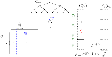
The catalog graph is a balanced binary tree of height . To be able to describe the sequence of insertions, we will use a geometric representation of our construction as follows. We measure the level of any vertex in from 1, for convenience. So, the root of has level while any vertex with distance to the root has level ; the leaves of have level . Let . We use the -axis to model the universe (i.e., the values in the catalogs) while the -axis will be used to capture the catalog graph . We map each vertex in to a rectangular region in . Partition into congruent “slabs” using vertical lines (i.e., vertical lines). Assign these rectangles to the vertices of at level , from left to right. In particular, the root of will be assigned the entire whereas the left child of the root will be assigned the left half of and so on. For a vertex , let be the rectangle assigned to . See Figure 1(left).
Observation 1.
For two vertices , and have non-empty intersection if and only if one of the vertices is an ancestor of the other one.
We will only insert integers between and into the catalog of vertices of . Assume, we have inserted values into the catalog of . Then, in our geometric view, we partition into sub-rectangles using horizontal lines at coordinates . See Figure 1(right).
Observation 2.
Let be a path from the root of to a leaf . Let be a (query) value in . Consider the pair as a fractional cascading query.
Let be the -coordinate of a point that the lies inside . Then, the fractional cascading query is equivalent to finding all the sub-rectangles that contain the query point .
In the rest of our proof, we will only consider fractional cascading queries that can be represented by such a query point . As we are aiming to prove a lower bound, this restriction is valid. Observe that in this view, the fractional cascading problem is essentially a (restricted form of) rectangle stabbing problem. We are now ready to define our sequence of insertions.
5.1 Parameters and Assumptions.
We will only consider data structures with polylogarithmic update times. Let be the update time of the data structure. Thus, . Shortly, we will describe our construction of difficult insertion sequences followed by a proof of why they are difficult. This will be done using a number of parameters; it is possible to read the proof without knowing the parameters in advance (in particular, at some point the author had to select the best parameters to obtain the highest lower bound), but probably it is more convenient to have their final values in mind so that one can have a “ballpark” notion of how large each parameter is. Let , and . and will be used in the construction, specifically, to define our insertion sequences. Observe that .
The list of other parameters that we use include the following. We set , and and is a sufficiently small constant. Our goal is to show a lower bound of for a fractional cascading query of length , meaning, will the multiplicative factor of our lower bound. We define and .
5.2 Details of the Construction
Our construction has epochs where at epoch , we will insert some values in the catalog of some vertices of . The value is fixed and known in advance, by the data structure.
We partition the vertices of into subsets that we call bands. The first levels of (i.e., the vertices in the top levels of ) are placed in the first band, the next levels are placed in the second band and so on. Overall, we get bands (for simplicity, we assume the division is an integer).
The vertices of the even bands (i.e., bands 2, 4, 6, etc.) will have their catalogs empty; we will never insert anything in vertices of these bands. Let be the number of odd bands.
To be more precise, the -th odd band consists of levels to . Initially all these levels are marked as untaken. During epoch , we select untaken levels, where is selected uniformly at random among all the untaken levels of the -th odd band. These levels then are marked as taken; this operation also comes with corresponding insertion sequences that we will define shortly. However, we have the following observation.
Observation 3.
In every epoch, and in every odd band, we have at most choices and at least choices for which level to take. Furthermore, the choices of different odd bands are independent.
Assume we are at epoch . Then, taking a level uniquely determines the sequence of values that we insert in the cataglogs of the vertices of level , as follows. Consider a vertex at level . We divide into congruent sub-rectangles which means we insert the -coordinates of their boundaries as values in the catalog of (Figure 1(right)).
Lemma 2.
During epoch , a total of values are inserted, independent of which levels are taken. Also, a sub-rectanble inserted during epoch at a vertex of level has height and width and area of .
Proof.
Assume we take a level and let be a vertex of level . As discussed, we divide into sub-rectangles, so each sub-rectangle is thus a rectangle of height and width with an area of .
As the number of vertices of level is , the total number of values that we insert at this level is ; this only depends on , the epoch and thus, over all the odd bands, we have values inserted. ∎
For the ease of presentation, we now define a notion epoch of change (EoC). Consider epoch . The sub-rectangles that we insert during this epoch are said to have EoC . Any memory cell that is updated during this epoch has its EoC sets to . Note that if a memory cell gets updated during epochs , then it will have EoC at the end. We use to denote the EoC of a memory cell .
6 Persistent Structures
6.1 The Existence Proof.
In this section, we consider the data structure after we have made all the insertions, at the end of epoch . Here, we choose to view the fractional cascading problem as the rectangle stabbing problem, as outlined by our geometric view, where a query is represented by a point . Observe that every query point is contained inside sub-rectangles and thus is the output size. Our ultimate goal is to show that the worst-case query time of the data structure is at least .
Let be a smallest directed tree explored at the query time that outputs all the sub-rectangles containing . Thus, contains cells that produce output; we call these, output cells. We call a subtree of that has output cells marked as output cells a -connector and its size is its number of vertices. Note that two connectors that have identical set of memory cells and edges are considered to be different if they have different subsets of cells marked as output. If there exists a query such that for every tree with output cells we have , then, the worst-case query time of the data structure is at least and thus we have nothing left to prove. As a result, in the rest of this proof we assume that for every qurey , there exists one tree of size less than .
The concept of “connectors” is a crucial part of static pointer machine lower bounds. However, this alone will not be sufficient for a dynamic lower bound. The problem is that we do not have any control on how these connectors are created. Ideally, we would like to be able to locate the same connector throughout the entire sequence of updates. To do that, we define the notions of strange and ordinary connectors. A connector is called strange if it contains two nodes and such that is an ancestor of (in the connector) and is an output node that outputs a sub-rectangle of EoC but is updated during a later epoch, meaning, . See Figure 2.
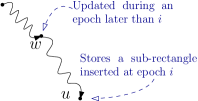
In plain English, the connector produces an output from an epoch using a memory cell that was updated in a later epoch . A connector that is not strange is called ordinary.
Ordinary connectors will be extremely useful later but at this point its not clear if such connectors even exist. In fact, for large values of , we can clearly see that ordinary -connectors may not exist: consider -connectors. Every query outputs exactly sub-rectangles, so is the only -connector in . However, always contains the root of the data structure, meaning, if the root is updated at every epoch, then there are no ordinary -connectors.
The main result of this section is that for an appropriate choice of , ordinary -connectors in fact exist. What we will prove is in fact slightly more complicated; we will show that for most queries , ordinary -connectors exist. To do that, we mark certain regions of as strange and we will show that as long as does not come from the strange region, then will contain an ordinary -connector.
6.2 Strange Regions.
In this subsection, we only consider the status of the data structure at the end of epoch . Let be this memory structure.
Marking regions.
This process uses a parameter , to be fixed later. To mark the strange region, we preform the following for every integer and every memory cell . Consider all the trees that can be made, starting from as their root and by following edges in . Let be one such tree. Consider all possible ways of marking the cells of as output cells. Let be a paritcular choice of output cells in . If each , stores a sub-rectangle such that and if , for a parameter , we mark as strange.
Our main lemma in this section is the following.
Lemma 3.
If , then the total area of the strange regions is .
Proof.
The number of insertions performed at epoch is by Lemma 2 and since we are working in the EWIA model, the number of memory cells of EoC is at most
| (1) |
Pick one memory cell with . Starting from and using edges, we can form at most subtrees . We can also mark the cells in as output or not in at most different ways. Thus, the total number of marked trees considered is
| (2) |
Following the definition of our marking process, let be one such tree and let be all the marked cells in . Assume that each , , stores a sub-rectangle such that , as otherwise, no region is marked strange. Assume is inserted in the catalog of a node at level . Observe that if then we do not increase the strange region. Thus, in the rest of this proof we only consider the case when . By Observation 1, this implies that all the nodes must lie on the same root to leaf path. Consequently, this implies all ’s are distinct. Assume was inserted at epoch . This means that is a rectangle with width and with height by Lemma 2.
W.l.o.g, let be the rectangle with minimum width and be the rectangle with the minimum height, i.e., and . We have, . Furthermore,
| (3) |
With a slight abuse of the notation and to reduce using extra variables, define and and note that the subscripts could refer to distinct or same sub-rectangles. Remember that we have and thus . Also we have and thus
| (4) |
and also since and ,
| (5) |
Remember that by our definitions, for every , we have and . Furthermore, as argued previously, the sub-rectangles have been inserted in nodes of that all lie on the same root to leaf path in . Additionally, if for two indices and we have , then it follows that the sub-rectangles and were inserted in the same epoch. But we only insert sub-rectangles into odd bands and between each two odd bands, there are at least levels. Thus, . Putting this all together, it follows that for each value of , , there can be at most sub-rectangles in the list . As a result, the maximum number of sub-rectanles in the list is , or in other words,
| (6) |
We now use inequalities (4) and (5) to obtain that
Also remember that we had . Thus,
| (7) |
We now consider two cases.
Case (i) .
As , by multiplying both sides with Equation (7) we get
| (8) |
Observe that we can plug in this inequality into Equation (3) and obtain that
| (9) |
We now calculate how much the strange region expands in this case. We need to sum over all choices of ( choices) and in each sum, we need to multiply the number of trees we consider given in Equation (2) and the area of increase given in Equation (9). So the increase in the area of the strange region is bounded by
| (10) |
where the first inequality uses the assumption that and the second inequality uses the fact that and the third inequality uses the observation that ; the observation can be verified for large enough if we plug in the value . Since we have less than epochs, the total increase of the area of the strange region is bounded by , in this case.
Case (ii) .
Here, we simply observe that
| (11) |
since and thus . As before, we can compute the total increase in the area of the strange region by summing over all choices of (less than choices) and in each sum, we need to multiply the number of trees we consider given in Equation (2) and the area of increase given in Equation (11). We obtain that increase is bounded by
| (12) |
where the last inequality uses that . As before, the total increase in the area of the strange region is bounded by . ∎
Lemma 4.
Let be a query point from the ordinary region of and let be the tree traversed at the query time such that . Let be a parameter such that where is the parameter used in Section 6.2. We can find a number, , of disjoint ordinary connectors such that the -th connector has output cells and has size at most with . Furthermore the connectors contain at least of the output cells.
Proof.
We first find a set of (initial) connectors iteratively, by cutting off subtrees of . Then, for each initial connector, we find a subset of it that is ordinary.
We find the initial set iteratively. In the -th iteration, if there are fewer than output cells left, then we are done. Otherwise, consider the lowest cell that has at least output cells in its subtree; as is a binary tree, has at most in its subtree as otherwise, one of its children will have at least output cells and will be lower than . Let be the number of output cells at subtree of and be its size. If , then we have found one initial connector, we add it to the list of initial connectors we have found and delete and its subtree and continue with the next iteration. However, if the subtree at is larger than , we call its output cells wasted and again we delete the subtree hanging at and then continue. Let be the total number of wasted cells and with a slight abuse of notation, let be the set of initial connectors that we have found where has output cells and has size . Observe that since each wasted cell can be charged to at least other cells in the tree and there are at moest cells in . Every output cell is either wasted, placed in a connector or it is among the fewer than output cells left at the end of our iterations. Thus,
Observe that the value is chosen such that the size of each initial connector is at most , satisfying the condition of Lemma 3. Consider one connector . If is ordinary, then we are done. Otherwise, we will “unmark” some of its output cells, meaning, we will obtain another connector that has the exact same set of edges and vertices as but whose set of output cells is a subset of the output cells of . This unmarking will make sure that is ordinary and furthermore, it still contains “almost” all of the output cells of .
We now focus on . Consider a cell . Let be the set of cells in the tree that is hanging off that conflict with , meaning, for each cell , . We unmark all the elements of , for every cell . The main challenge is to show that at least a fraction of the output cells of survive this unmarking operation. Nonetheless, it is obvious that is ordinary (note that could have no output cells, in which case it is still ordinary).
Let be the set of cells in that have conflicts, i.e., includes all the cells such that .
Consider two nodes and such that is an ancestor of . Observe that if , then : consider a cell . By definition, is in the subtree of and thus also in the subtree of and furthermore, we have but since , we also have and thus . This means that we can essentially ignore the unmarking operation on as will take care of those conflicts. We now “clean up” by removing any such cells from .
As a consequence, we can now assume that has the following property: for every two cells and in where is an ancestor of , we have .
We now consider an iterative unmarking operation. Let be the memory cell in that is closest to the root of . Let be the cells in that belong to the subtree of . Since we have cleaned up , it follows that . Let . We now make two claims.
Claim (i).
For every cell , is not contained in the subtrees of : this claim is easily verified since if is in the subtree for some , then we must have and thus also belongs to which is a contradiction with the assumption that .
Claim (ii).
Let be the set of cells that is the union of all the paths that connect to for all . We claim : This claim follows because of the way the strange regions are marked in Subsection 6.2; we have and thus is less than or equal than , the parameter we used in marking the strange region. This means that, at some point during the process of marking strange regions, we would consider the cell and the tree with root that is formed by exactly the of edges in . Also, at some point we consider exactly the set as the marked cells of . Now, if then we would mark the intersection of all the sub-rectangles of as strange which in return implies that is inside the strange region, a contradiction. Thus, . We now unmark the cells and charge this operation to ; by what we have just said, every edge in receives at most charge.
Now observe that we can remove from . All the other cells that have conflict with will be unmarked by other cells in , by the definition of . We continue the iterative unmarking operation by taking the next highest cell and so on. This operation unmarks all the conflicting cells and thus leaves us with an ordinary connector. Furthermore, each unmarking operation, charges some edges of with charge. We claim each edge receives at most one charge and to do that, we simply observe that for two cells and , the sets and are disjoint. Assume w.l.o.g, that was selected first and that were the highest cells in in the subtree of . Now observe that must either lie outside the subtee of or it must lie in the subtree of one of the cells , revealing that and are disjoint.
Thus, if is the total number of cells that get unmarked by this operation, we must have . Thus, at most output cells are unmarked to obtain an ordinary connector of size at least
In addition, over all the indices , the total number of output cells that are unmarked is
Now the lemma follows since every output cell is either wasted, unmarked or is among the left over cells. ∎
6.3 The Structure of an Ordinary Connector.
Let be the memory graph at the end of epoch . Let us review what Lemma 4 gets us. First, observe that by the choice of our parameters, we have (by having in the definition of small enough). Second, recall that the output size of any query is and furthermore, we have assumed that every query can be answered by traversing a subtree of of size at most . By Lemma 4, we can set and decompose into ordinary connectors of size between and . Crucially, in doing so, we only need to leave out at most output elements. As a result, for every query point that is not in the strange region, there exists a ordinary -connector of size at most , with , whose output sub-rectangles contain and at least one of its sub-rectangles has been inserted no later than epoch . Pick one such connector and call it the main ordinary connector of . Let be the earliest epoch from which has an output cell. To simplify the analysis later, we assume has exactly output cells from epoch ; for now, we treat the integers and fixed, i.e., we only consider ordinary connectors with exactly output cells from epoch . In addition, from now on, we will only focus on the main ordinary connectors.
The fact that is ordinary yields very important and crucial properties that are captured below, but intuitively, it implies that we can decompose into “growth spurts” where during each growth spurt, it “grows” a number of branches.
Let , for , be the set of output cells that store sub-rectangles that belong to epoch (i.e., they were inserted during epoch ). Let be the root of . The younger at time , is defined as the union of all the paths that connect cells of to ; by the ordinariness of , the subgraph existed at the end of epoch and it has not been updated since then; this structure has been preserved throughout the later updates. The -th growth spurt, , is defined as where is an empty set. Observe that is a forest and we call each tree in it a branch. We call the edge that connects a branch to a bridge. For a cell in a branch, we define the connecting path of to be the path in that connects to its bridge. If a branch has at least edges, for a parameter , we call it a large branch otherwise it is a small branch. For every output cell in , consider the connecting path of that connects to a cell adjacent to its bridge. We define the bud of to be the first cell on path (in the direction of to ) which is updated in epoch . Observe that since is ordinary, bud of exists but it is possible for an output cell to be its own bud. See Figure 3.

6.3.1 Encoding an Ordinary Connector.
We now try to represent the main ordinary connector of any query , together with most of the information given above, as a bit-vector, . We assume that every cell has two out-going edges (by adding dummy edges) and one of them is labelled as the “left edge” while the other one is marked as the “right edge”. We assume this marking does not change unless the algorithm updates the memory cell. For a given ordinary connector with root , the bit-vector encodes the following: (i) the shape of , i.e., starting from and in DFS ordering of , for every cell , we use two bits to encode whether the left or right edge going out of belongs to (ii) the number of output cells from each epoch, (iii) for every edge we encode whether it’s a bridge or not, (iv) for every cell in we encode whether it’s an output cell, and/or a bud (v) we encode which branches belong to epoch , and finally, (vi) for every large branch we encode the epoch it belongs to. Note that omits some major information: for output cells that belong to small branches, we do not encode the epoch they belong to. Also, note that from (i) and (vi), we can deduce the exact number, , of the output cells of epoch that are on the small branches.
Lemma 5.
Let be an ordinary -connector of size . Then, at most bits are required in .
Proof.
Let . Encoding (i) requires bits, for (iii), (iv), and (v) we require at most bits per cell, for a total of bits. Note that a partition of into branches is uniquely determined by the set of bridges.
Now consider large branches; as each large branch contains at least edges, the total number of large branches is at most . Encoding the epoch requires bits and thus (vi) requires at most bits (recall that ).
Finally, (ii) requires bits, since it is equivalent to the problem of distributing identical balls into distinct bins. Thus, in total we need bits. ∎
7 The Lower Bound Proof
7.1 Definitions.
We use the notation to denote the memory graph at the end of epoch . denotes the memory graph at the beginning of the first epoch. Consider an epoch . Consider a string that is the valid encoding of an ordinary connector. Recall that at all times, for every cell its two out-going edges are labelled as left and right. This implies that for every cell , the string uniquely identifies a connected subgraph formed by taking exactly the edges encoded by . We denote this by and note that this maybe not be a tree or even a simple graph.
During each epoch, a region of is marked as forbidden. We always add a region to the forbidden region, never remove anything from the forbidden region. Another way of saying this is that the forbidden region always expands, i.e., the forbidden region at the end of epoch will contain the forbidden region at the end of epoch . At the end of epoch , the query that we will ask will not be in the forbidden region (also it will not be in the strange region). We will keep the invariant that the forbidden region is a small fraction of . In addition, for a region and at an epoch , we may conditionally forbid (CF) at a cell . This implies the following. If at any later epoch , the cell or any cell in the -in-neighborhood of is updated by the algorithm, then the region is added to the forbidden region. For ease of description, we sometimes say that is CF at the beginning of epoch , which is equivalent to being CF at the end of epoch .
We now describe the forbidden regions.
7.1.1 The First Type of Forbidden Regions.
Recall the details of our construction: at each epoch, we take levels, one level in each odd band. Depending on which levels we take, we insert a different sequence of sub-rectangles in the data structure.
Definition 1.
Consider the beginning of epoch and . For each vertex we assign to a set of sub-rectangles as tags as follows. Assume there is a choice of levels to take in epoch that results in an insertion sequence that leads to the following: at the end of epoch , the algorithm has updated the cell (its contents or pointers) and it has stored a sub-rectangle that was inserted in epoch at a memory cell in the -out-neighborhood of . Then we add as a tag to the set of tags of .
The set of tags of a cell is thus determined at the beginning of epoch . At the beginning of epoch , we consider the (geometric) arrangement of the tags of . We add any point that is contained in more than tags to the forbidden region.
Lemma 6.
The area of the first type of forbidden regions is increased by at every epoch.
Proof.
Recall the details of our construction and remember that at each epoch , we take levels among the untaken levels of each odd band. By Observation 3, in each odd band we have at most choices. Over odd bands this adds up to at most choices for which levels to take. As the size of -out-neighborhood of is at most , the number of sub-rectangles added to as tags is at most . The number of geometric cells in the arrangement is at most .
Consider a geometric cell that is contained in sub-rectangles in . By Observation 1, for to have non-empty intersection, they all must belong to the same root to leaf path in , i.e., must have different levels. Thus, w.l.o.g, assume the sub-rectangles are sorted by the increasing value of their levels. As a result, if is the level of and is the level of , we must have . By Lemma 2, is a rectangle of height and width and is a rectangle of height and width . As a result,
Thus, if we consider the arrangement , every geometric cell that is contained in sub-rectangles will have an area of at most by above, meaning, in total can have an area of
| (13) |
in such cells.
Finally, observe that we only consider cells that are updated by the algorithm. By Lemma 2, during epoch , a total of values are inserted, and since we are operating in the EWIA model, this means that a total of cells can be updated; multiplying this by Equation 13 reveals that the total increase in the area of the forbidden region is bounded by
∎
7.1.2 The Second Type of Forbidden Regions
Definition 2.
Let be a cell that is updated during epoch . If a cell in the -out-neighborhood of stores a sub-rectangle that is inserted in the previous epochs (i.e., epochs to ), then we add to the forbidden region.
Lemma 7.
The area of the second type of forbidden regions is increased by at every epoch.
Proof.
Observe that the area of is at most by Lemma 2. However, during epoch , we insert values. Since we are operating in the EWIA model, this means that the data structure can modify at most memory cells . The size of the -out-cone of is at most and thus in total we can increase the area of the forbidden region by
by the definition of . ∎
7.1.3 The Third Type of Forbidden Regions
Definition 3.
Let be a cell that is updated during epoch . If there is a cell in the -out-neighborhood of , such that a region is conditionally forbidden at , then we add to the forbidden region.
Lemma 8.
If each cell contain a conditionally forbidden region of area at most , then the area of the third type of forbidden regions is increased by at every epoch.
Proof.
The proof is very similar to the previous lemma: during epoch , the data structure can modify at most memory cells . The size of the -out-cone of is at most . Thus, we can increase the area of the forbidden region by
by the definition of . ∎
7.1.4 Living Trees.
At each epoch, we will maintain a set of living trees. In particular, every memory cell will have a set of living trees with as their root. Note that this set could be empty. A living tree is defined with respect to a string that encodes a (main) ordinary connector and a root cell . A living tree (at the end of epoch ) must be a subtree of . Unlike , a living tree must be a tree. Informally speaking, a living tree is tree that has the potential to “grow” into a ordinary connector by the end of epoch , so, it should not contradict the encoding .
Definition 4.
More formally, we require the following: a living tree should be a subtree of , and it must have as its root. should be ordinary, and it should be consistent with encoding , both in its structure and its number of output cells. To be more specific, must contain all the long branches belonging to epochs and before (as encoded by ) with correct sub-rectangles stored at their output cells (i.e., if a long branch is marked to belong to epoch , , a sub-rectangle inserted during epoch must be stored at its output cells). For every small branch encoded by , should either fully contain it or be disjoint from it. If contains a small branch, then a sub-rectangle inserted at an epoch , , must be stored in its output cells. Furthermore, must have exactly output cells on small branches that belong to epoch , where is the number (implicitly) encoded by , for every . In addition, should be the encoding of a main connector, meaning, for , should have no output cells from epoch but exactly output cells from epoch . Finally, for every output cell in , its bud should be at the correct position, as encoded by . In this case, we say super-encodes .
We need to remark that by the above definition, there are no living trees before epoch .
Definition 5.
Consider a living tree at the end of epoch . Remove all the branches that contain output cells that belong to epoch . We obtain a living tree at the beginning of epoch and we say that is grown out of . In addition, if we have a sequence of living trees in epochs , , …, respectively, where each living tree is grown out of the preceding one, then we can also say is grown out of (in epoch ).
Definition 6.
Consider a living tree with super-encoding and the connected graph . While may not be a tree during epoch , nonetheless, includes the encoding of branches that are connected to via bridges. We call those the adjacent branches of . We can use the quantifier small or large as appropriate to refer to those branches. Similarly, an adjacent output cell is one that is located on an adjacent branch. And same holds for an adjacent bud.
Some intuition.
The following two definitions are a bit technical. However, the main intuition is the following. Consider an ordinary -connector at the end of epoch . Let be the sub-rectangles stored at the output cells of . We would like to define the region of as the intersection of all the sub-rectangles since if is the main connector of a point , then clearly and thus the notion of “region” will represent the subset of for which this connector can be useful. The same idea can also be defined for the living trees. Then, our next idea is to define a potential function which is the sum of the areas of the regions of all the living trees. And then, our final maneuver would be to show that this potential function decreases very rapidly every epoch, and thus by the end of epoch , it is too small to be able to cover all the points in . However, one technical problem is that to show this decrease in the potential function, we need to disregard and discount some small subset of ; the concept of “forbidden region” does this. But this also necessitates introducing a “dead” region for each living tree so that we can define the region of a living tree as the intersection of its output sub-rectangles minus its “dead” region. And finally, the intuition behind the dead region is the following: consider a point and a living tree in epoch . Assume, during epoch we can already tell that no matter how grows into a main ordinary connector in epoch , is always added to the forbidden region. In this case, in epoch we mark as “dead” in advance and thus stop counting it in our potential function. We now present the actual definitions.
Definition 7.
Consider a living tree at the end of epoch with super-encoding . will be assigned two geometric regions and and a value . is defined as the area of . is defined inductively as follows, and it depends on as follows.
Note that before epoch , there are no living trees, as we are only concerned with the main ordinary connectors. At epoch , the string exactly encodes the location of the small and large branches that belong to this epoch, as well as the locations of their output cells; as is living, all such output cells contain sub-rectangles inserted during epoch ; is defined as the intersection of all such sub-rectangles and here is empty.
During any later epoch , , is defined using for a living tree in epoch from which grows. By definition, grows out of by adding a number of small branches that collectively contain small output cells that store sub-rectangles . Then, we may assign a dead region to , denoted by . always contains the entirety of the current forbidden region but it might contain more regions. We then define .
We now make the intuition that we had about the dead region into an explicit invariant that we will keep.
The dead invariant.
Consider a living tree in epoch with super-encoding and a point . Then, over the choices of the future levels that we may take (in our construction) and modifications that the data structure can make to the memory graph, it is not possible for to grow into an ordinary connector connector with encoding such that is contained in all the output sub-rectangles of but outside the forbidden region.
We now consider a particular way we can expand the dead region of a living tree.
Definition 8.
Consider a living tree in the beginning of epoch with super-encoding and root . Let be a living tree at the end of epoch that has grown out of . Let be the integer that describes the number of output cells of on small branches in epoch , as encoded by .
Observe that all the large branches that belong to epoch (as encoded by ) must be adjacent to and furthermore, every output cell of them must be updated with a sub-rectangle inserted during epoch as otherwise no living tree can grow out of . Let be those sub-rectangles. Let be the sub-rectangles inserted during epoch in the output cells of adjacent small branches of . Observe that we must have or else no living tree can grow out of . can grow out of by adding all the large branches that contain and some number of small branches that collectively contain output cells. W.l.o.g, assume are those output cells. Let be the forbidden region at the end of epoch . We add to .
Observation 4.
The process in Definition 8 respects the dead invariant.
Proof.
Consider the notation used in the definition. If then clearly will be in the forbidden region by the end of epoch since the forbidden region always expands. Let and let be the output cell that stores . Thus, consider the case when ; other cases follow identically. Observe that by assumptions, does not include the output vertex . If never grows into an ordinary connector with encoding , then we are done. Otherwise, according to encoding , at some point should become an output cell. This means that at some point in the future, a cell on the connecting path of should be updated. However, by the second type of forbidden regions outlined in Definition 2, this means that will be added to the forbidden region and since , thus will be added to the forbidden region as well. Thus, our dead invariant is respected. ∎
Lemma 9.
Consider a living tree in epoch and let be the living trees in epoch that grow out of . Then, have pairwise disjoint regions. Also, .
Proof.
Consider the notation used in Definition 8. Consider the geometric arrangement created by the rectangles and . Observe for any tree that grows out of , the region is contained in all the and exactly of the sub-rectangles of and furthermore, those sub-rectangles are stored at of the output cells of . As a result, any other living tree must have a different subset of sub-rectangles at its output cells, meaning, its region will be disjoint from , because of the way the dead region is defined in Definition 8. This shows that all the regions are pairwise disjoint. The second part follows since by definition we have . ∎
Observation 5.
Let be living trees with root and super-encoding . Then, they have pairwise disjoint regions.
Proof.
The proof is an easy induction. By the definition of living trees and string , there is exactly one living tree at epoch . Assume the claim holds for epoch , . Then by Lemma 9 it also holds for epoch . ∎
The previous observation allows us to simplify and streamline our view of the living trees. Recall that . We partition into pixels where each pixel is a unit square with integer coordinates. A pixilated living tree (PLT) is a pair of where is a living tree and is a pixel such that . We define . By Observation 5, we can decompose all the living trees with root and with super-encoding into a number of PLTs that have disjoint pixels (regions). By Observation 5 and Lemma 9, if a PLT grows into a PLT then and is a living tree that grows out of by adding output cells, located on small branches, according to encoding . In this case, with a slight abuse of the notation we can say survives until the next epoch, however, it is more accurate to say that it grows. However, when is added to the dead region, forbidden region or if it lies outside the sub-rectangles inserted at the output cells of , then we have that and thus PLT does not survive the epoch.
Definition 9.
Consider a fixed string and a PLT in with super-encoding and root . For a cell , if the following conditions hold, then we say is relevant to : We must have , , must be marked as a bud according to string .
For technical reasons, for every PLT we need to keep track of a certain value, that we call the depleted count (DC). Informally, it counts the number of cells on the adjacent branches of that can no longer be updated, if were to survive until the end of epoch . This will be clarified later. What we need to know at this point is that the DC of a PLT can never decrease, as we progress through the epochs. Initially, i.e., at epoch , all PLTs have DC 0.
Definition 10.
Consider the beginning of epoch and let and be two integers. Define as the set of all PLTs that have DC and have a total of output cells in epochs 1 to , located on the small branches 444To unclutter the notation, we have not reflected the dependency of on the integer ..
Definition 11.
Consider a cell . Let . For integers , , we define the following:
| (14) |
| (15) |
| (16) |
And finally, we set .
Note that in Equation (15) is always 1 but we have avoided this substitution to emphasize that we are computing the total area covered by all the PLTs.
Definition 12.
Consider and two fixed values and . We categorize every cell as one of the following three cases, using two values , and .
-
•
If then we call a -tiny cell.
-
•
If then we call a -fit cell.
-
•
Finally, if then we call a -oversized cell.
Definition 13.
Consider a cell . We define a function from to where for a point , is the number of regions in that contain the point . The dense subset of , denoted by , is the subset of of area at most that contains the largest values of the function, meaning, for every point and every point we have .
If is not -oversized, then but if is -oversized, then has area .
Finally, the following operations are performed at the beginning of each epoch.
Definition 14.
At the beginning of epoch , and for every do the following.
-
•
(default marking) If for some and , , is a -tiny cell, then we conditionally forbid at . If is -fit, we conditionally forbid at at epoch . If is -oversized, we conditionally forbid at at epoch .
-
•
(fit marking) If for some and , , is a -fit cell, we do the following. At the beginning of epoch , we “assign” to to be later conditionally forbidden. Thus, at the beginning of epoch , each cell will have an “assigned” region. Then, in epochs until , every time the data structure updates a cell , all the regions that are assigned to cells in the -out-neighborhood of are added to the region assigned to . At epoch , all the regions assigned to the cells are conditionally forbidden.
-
•
(dense marking) If for some and , , is an -oversized cell, then we repeat the above process (the process for the fit cells) but only for .
We now bound the total area we conditionally forbid at each epoch using the above processes. First consider the default marking process. If is -tiny, then it CF an area of at most over all choices of and . Otherwise, an area of at most is CF, over all choices of and but at epoch but this is allowed by Lemma 8. The fit marking is a bit more complicated. Observe that at the beginning of epoch , each cell is assigned an area of at most (over all choices of and ). Whenever the algorithm updates a node , then the regions assigned to all the cells in the -out-neighborhood of are added to the assigned region of ; this can increase the assigned area of by at most a factor (the size of -out-neighborhood of ). This process continues for epochs, meaning, by epoch , the assigned area of each node can be as large as . However, observe that these cells are conditionally forbidden at epoch . But in epoch , we are allowed to have an area of conditionally forbidden at each cell, by Lemma 8. Observe that
and thus this is well within the condition specified in Lemma 8. The case of dense marking is exactly identical to this case.
7.2 A Potential Function Argument.
Our final analysis is in the form of a potential function argument. We in fact define a series of potential functions.
Definition 15.
For integers and , , and in (i.e., the beginning of epoch ) we define a potential function as follows:
| (17) |
Observation 6.
We have
Proof.
Consider a PLT (i.e., with output cells and DC ). The area of is added to , for cells since has adjacent buds. ∎
However, before getting to the potential function analysis, we need to investigate how a living tree in epoch can grow into a living tree in the future epochs. Let be a PLT tree with super-encoding at the beginning of epoch with DC . By definition, has output cells, located on small branches. We would like to calculate the probability of surviving in the next epoch, assuming it needs to add output cells that are located on the small branches, where is the integer encoded by string . Note that we completely ignore the long branches; the string exactly encodes their location and we assume the data structure always places a suitable sub-rectangle there.
Let be the adjacent buds of that are located on the small branches. We have essentially four cases and we analyze each in a different subsection.
7.2.1 An adjacent small bud of is -tiny.
Lemma 10.
If any of the cells is -tiny, then cannot survive until epoch .
Proof.
W.l.o.g., assume is -tiny. is located on an adjacent small branch which means its connecting path has length at most . In addition, recall that the region of every tiny cell has been conditionally forbidden at the beginning of the epoch (by the default marking process) Since, is contained in , it thus follows that has been conditionally forbidden. As a consequence, if the data structure updates any of the cells on the connecting path of , is added to the forbidden region. On the other hand, according to string , is marked as a bud and thus eventually it should be updated to lead to an output cell, a contradiction. ∎
Thus, in this case, we immediately and in advance add to the dead region, consistent with the dead invariant. As a consequence, we can assume that none of the cells is -tiny, meaning, they are either -fit or -oversized.
7.2.2 Too many fit cells and dense areas.
Lemma 11.
Assume there exists at least cells , among the cells , such that either (i) is -fit or (ii) is -oversized and . Assume survives the epoch . Then, there are at least cells, , among the cells with following property: has a cell on its connecting path such that if any of the cells on the connecting path of is updated, then is added to the forbidden region.
Proof.
W.l.o.g, let be the cells that satisfy condition (i) or (ii) outlined in the lemma.
Consider the epochs to . We claim, during each of these epochs, can grow by at most output cells; assume during one epoch grow by at least output cells, that store sub-rectangles. However, in each epoch, we take exactly levels, one in each odd band. This implies that at least two of the sub-rectangles must be in the same level and thus they have empty intersection. As a result, it follows that grows into a PLT with an empty region, a contradiction. Thus, during epochs to , can grow by at most output cells, leaving at least cells among still in the adjacent branches.
Consider one of those cells and consider the fit marking and the dense marking process in Definition 14. Consider the connecting path of in epoch . Let be the cell farthest from in that is updated during epochs to . Recall that by the default marking process, if is -fit (resp. -oversized) we CF (resp. ) at and also recall that by our assumptions (resp. ). As a result, if does not exist, then by the default marking process, is CF at and thus the data structure cannot update or any of the cells in its connecting path without adding to the forbidden region, meaning, cannot survive until epoch . Otherwise, by the fit marking and the dense marking processes, is conditionally forbidden at epoch at . The cells are the cells claimed in the lemma. ∎
In this case, we increase the DC of and this is the only way the DC of a PLT can increase: at epoch , we can consider the cells as “depleted” and to reflect that, the DC of is increased by . One technical issue that we need to outline here is the DC does not count the number of distinct depleted cells as we could have for to different cells and . Instead, DC counts the number of depleted cells with multiplicity. To make the later analysis easier, we can bound this as follows. If a PLT satisfies the conditions in Lemma 11, we increase its DC by but assume it can grow without any restrictions until epoch . This idea will come handy later when we are trying to analyze our potential function.
7.2.3 Growth Using Fit or Dense Areas
Lemma 12.
Consider a PLT with super-encoding . Consider a point and assume it has not been marked dead in this epoch. Consider the cells such that either (i) is -fit or (ii) is -oversized and . W.l.o.g, let be all such cells.
When , the probability that survives by the end of epoch and grows by additional output cells, using only cells is at most ; is the number of output cells that must belong to epoch , on the small branches, as encoded by .
Proof.
Let be the pixel associated with . Let us review our progress: by Lemma 10, none of the cells can be -tiny.
Consider a cell , among the cells . Since we are working with encoding , for to grow using , should become a bud, meaning, the data structure must update but none of the cells on the connecting path of . Furthermore, after updating , the data structure has to store a sub-rectangle at the position of the output cell of , with (if then does not survive, by the definition of ). This in turn implies that exists as a tag (see Definition 1 on page 1) in the arrangement of tags, , defined during the first type of forbidden regions.
Next, recall that when we defined the first type of forbidden regions, we added any point that is contained in more than tags to the forbidden region. As a result, the sub-rectangle can only be one of the possible sub-rectangles in that contain the pixel . Let be the set of sub-rectangles in the arrangement that contain the pixel .
It now remains to make one crucial but almost trivial observation: a necessary condition for a sub-rectangle to be stored anywhere by the data structure is that it must be inserted in the insertion sequence! And a necessary condition for the latter is that a particular level must be taken, among the untaken levels in our construction. Furthermore, as any set of distinct sub-rectangles with non-empty intersection correspond to sub-rectangles inserted on distinct odd bands, it follows that the probability that we insert any fixed set of sub-rectangles in our insertion sequence is at most , by Observation 3.
The number of different ways we can select sets among the sets and then select distinct sub-rectangles, one from each selected set, is at most and thus the probability that is contained in the intersection of sub-rectangles is bounded by
according to our choice of parameters. ∎
7.2.4 Using Oversized Cells.
Consider the memory graph and consider a -oversized cell . We bound how much the “not dense part of” can help the growth of the PLTs.
Lemma 13.
Consider the beginning of epoch and the graph . Let be a -oversized cell. Let contain all the PLTs that satisfy the following: is a PLT at the end of epoch , has grown out of a PLT (at the beginning of epoch ) by adding a branch with as a bud, and (here, and are considered at the beginning of epoch ). Then, .
Proof.
Let be the union of all the sub-rectangles in the -out-neighborhood of inserted during epoch . We begin by bounding the following:
| (18) |
Consider a PLT (at the end of epoch ) with super-encoding that has grown out of a PLT (at the beginning of epoch ), by adding as a bud. Observe that in , bud uniquely identifies a memory cell in the -out-neighborhood of that is the output cell which stores a sub-rectangle inserted during epoch . By definition of and , we have . But we must also have . As a result, .
Recall that by definition of function , for a point , counts how many living tree have . As a result, we can rewrite Eq. 18 as follows:
| (19) |
As is -oversized, we have, . By definition of ,
| (20) |
We rewrite (20) as
Next, observe that for every point and every point we have , by the definition of . As a result,
Thus,
| (21) |
7.3 The Potential Function Analysis.
Let be the random variable that represents the set of choices (of which level to take) during epochs 1 to and let be one particular set of choices. Recall that the potential function was defined as
Note that the potential function is in fact a random variable that depends on . We use the bold math font to highlight this, e.g., when the potential is a random variable we represent it with . Thus, is simply a fixed value and not a random variable. Let for . We estimate based on these values.
Consider a PLT at the end of epoch that is counted in . We have the following cases:
- •
-
•
(case 2: via Lemma 12) Otherwise, if is grown out of a PLT in epoch that satisfied the conditions of Lemma 12, then we count in this case. Let be the part of the potential that falls in this case. By Lemma 12 we have,
(23) Note that this case also counts the case when , i.e., does not grow and does not gain additional output cells.
- •
Observe that the right hand side of Equation (24) is asymptotically bounded by the right hand side of Equation (23). Thus, by adding up Equation (22), Equation (23), and Equation (24) and taking the expectation over the choices of , we get the following recursion
| (25) |
where is some constant (it comes from the fact that we have absorbed Equation (24) into Equation (23)).
Now it is time to revisit the concept of main ordinary connectors and see what are the initial values of these recursive functions. Recall that any main ordinary connector has output cells from epoch and we have . Now consider epoch . We have , as long as . So we upper bound . To that end, we simply count the maximum number of living trees we can have in epoch . We have choices for the root of . The number of strings is at most by Lemma 5. Finally, of each living tree is at most , since by Lemma 2, the area of any sub-rectangle inserted during epoch is . Let .
Thus, we can obtain the following initial values for the potential functions:
| (26) |
Solving Equation (25) is a bit difficult. However, we can use induction. First, we consider the case when and observe that the 2nd summation disappears (since DC cannot be negative) and we are left with the following recursion:
| (27) |
We guess that
| (28) |
We can simply plug this guess and verify:
| (29) |
where in the last step, we are using that
is a known binomial identity 555For a quick proof, observe that the left hand size counts how many ways one can select numbers among numbers to by first selecting the maximum value, , then selecting the remaining elements from to .. Having the value of , we can now work out the value of , as we can now replace a value for the second summation in Equation (25). This forms the basis of our induction argument. We guess that
| (30) |
and thus we would like to bound .
| (31) | ||||
| (32) |
We bound each of the sums separately and for clarity:
| (31) | |||
| (32) | |||
Thus,
| (33) |
as claimed.
We are now almost done. Let be the subset of that lies outside the forbidden and strange regions. Recall that the total area of the forbidden and the strange regions is and thus the area of is . Because of the dead invariant, any point , must be contained in the where is a main connector of with some values of and . Consequently, there are values of and for which the total area of over all the main connectors that have exactly outputs from epoch is at least . In addition, any such connector must have at least output cells and at least output cells that lie on small branches. Also, for each connector the DC can be at most and thus the parameter in Equation (33) can be at most . Thus, by Equation (33), the expected area of such connectors is bounded by . As , and , it follows that
by setting small enough. This leads to a contradiction since we expected the total area of over all the main connectors to have area .
Thus, we have proven the following theorem.
Theorem 1.
If a fully dynamic pointer machine data structure with amortized update time, or an incremental pointer machine data structure with worst-case update time can answer fractional cascading queries on a subgraph in time in the worst-case, then, we must have .
8 Acknowledgements
The author would like to thank Seth Pettie for the encouragements he provided throughout the years he has been working on this problem.
References
- [1] Peyman Afshani. Improved pointer machine and I/O lower bounds for simplex range reporting and related problems. In Symposium on Computational Geometry (SoCG), pages 339–346, 2012.
- [2] Peyman Afshani, Lars Arge, and Kasper Dalgaard Larsen. Orthogonal range reporting: query lower bounds, optimal structures in 3-d, and higher-dimensional improvements. In Symposium on Computational Geometry (SoCG), pages 240–246, 2010.
- [3] Peyman Afshani, Lars Arge, and Kasper Green Larsen. Higher-dimensional orthogonal range reporting and rectangle stabbing in the pointer machine model. In Symposium on Computational Geometry (SoCG), pages 323–332, 2012.
- [4] Peyman Afshani and Pingan Cheng. 2D fractional cascading on axis-aligned planar subdivisions. to appear in FoCS, 2020.
- [5] Peyman Afshani and Anne Driemel. On the complexity of range searching among curves. In Proceedings of the Annual ACM-SIAM Symposium on Discrete Algorithms (SODA), pages 898–917, 2017.
- [6] Peyman Afshani and Jesper Sindahl Nielsen. Data Structure Lower Bounds for Document Indexing Problems. In International Colloquium on Automata, Languages and Programming (ICALP), volume 55, pages 93:1–93:15, 2016.
- [7] Peyman Afshani, Ingo van Duijn, Rasmus Killmann, and Jesper Sindahl Nielsen. A Lower Bound for Jumbled Indexing, pages 592–606. 2020.
- [8] Lars Arge, Vasilis Samoladas, and Ke Yi. Optimal external-memory planar point enclosure. In Proceedings of European Symposium on Algorithms (ESA), pages 40–52, 2004.
- [9] Mikhail J. Atallah, Richard Cole, and Michael T. Goodrich. Cascading divide-and-conquer: A technique for designing parallel algorithms. SIAM Journal of Computing, 18(3):499–532, 1989.
- [10] Lech Banachowski. A complement to Tarjan’s result about the lower bound on the complexity of the set union problem. Information Processing Letters (IPL), 11(2):59 – 65, 1980.
- [11] Bernard Chazelle. Filtering search: A new approach to query-answering. SIAM Journal of Computing, 15(3):703–724, 1986.
- [12] Bernard Chazelle. Lower bounds for orthogonal range searching: I. the reporting case. Journal of the ACM (JACM), 37(2):200–212, 1990.
- [13] Bernard Chazelle and Leonidas J. Guibas. Fractional cascading: I. A data structuring technique. Algorithmica, 1:133–162, 1986.
- [14] Bernard Chazelle and Leonidas J. Guibas. Fractional cascading: II. Applications. Algorithmica, 1:163–191, 1986.
- [15] Bernard Chazelle and Ding Liu. Lower bounds for intersection searching and fractional cascading in higher dimension. Journal of Computer and System Sciences (JCSS), 68(2):269–284, 2004.
- [16] Bernard Chazelle and Burton Rosenberg. Simplex range reporting on a pointer machine. Computational Geometry, 5(5):237 – 247, 1996.
- [17] Vincent Cohen-Addad, Laurent Feuilloley, and Tatiana Starikovskaya. Lower bounds for text indexing with mismatches and differences. In Proceedings of the Annual ACM-SIAM Symposium on Discrete Algorithms (SODA), pages 1146–1164, 2019.
- [18] Richard Cole. Parallel merge sort. SIAM Journal of Computing, 17(4):770–785, 1988.
- [19] Paul F. Dietz and Rajeev Raman. Persistence, amortization and randomization. In Proceedings of the Annual ACM-SIAM Symposium on Discrete Algorithms (SODA), page 78–88, 1991.
- [20] Yoav Giora and Haim Kaplan. Optimal dynamic vertical ray shooting in rectilinear planar subdivisions. ACM Transactions on Algorithms (TALG), 5(3), 2009.
- [21] Joseph M. Hellerstein, Elias Koutsoupias, Daniel P. Miranker, Christos H. Papadimitriou, and Vasilis Samoladas. On a model of indexability and its bounds for range queries. Journal of the ACM (JACM), 49(1):35–55, 2002.
- [22] Kurt Mehlhorn, Stefan Näher, and Helmut Alt. A lower bound on the complexity of the union-split-find problem. SIAM Journal of Computing, 17, 1988.
- [23] Kurt Mehlhorn and Stefan Näher. Dynamic fractional cascading. Algorithmica, 5(2):215–241, 1990.
- [24] Wolfgang Mulzer. A note on predecessor searching in the pointer machine model. Information Processing Letters (IPL), 109(13):726 – 729, 2009.
- [25] Han La Poutré. Lower bounds for the union–find and the split–find problem on pointer machines. Journal of Computer and System Sciences (JCSS), 52(1):87 – 99, 1996.
- [26] Robert E. Tarjan and Jan van Leeuwen. Worst-case analysis of set union algorithms. Journal of the ACM (JACM), 31(2):245–281, 1984.
- [27] Robert Endre Tarjan. A class of algorithms which require nonlinear time to maintain disjoint sets. Journal of Computer and System Sciences (JCSS), 18(2):110 – 127, 1979.
- [28] V.K Vaishnavi and D Wood. Rectilinear line segment intersection, layered segment trees, and dynamization. Journal of Algorithms, 3(2):160 – 176, 1982.
- [29] Dan E. Willard. New data structures for orthogonal range queries. SIAM Journal of Computing, 14:232–253, 1985.
Appendix A From Worst-case to Amortized Lower Bounds
In this section we prove a general reduction that shows under some conditions, we can generalize a query lower bound for an incremental data structure with a worst-case update time to a query lower bound for a fully dynamic data structure but with the amortized update time. The exact specification of the reduction is given below.
We work with the following definition of amortization. We say that an algorithm or data structure has an amortized cost of , for a function , if for any sequence of operations, the total time of performing the sequence of operations is at most .
We call the following adversary, an Epoch-Based Worst-Case Incremental Adversary (EWIA) with update restriction ; here is an increasing function. The adversary works as follows. We begin with an empty data structure containing no elements and then the adversary reveals an integer and they announce that they will insert elements over epochs. Next, the adversary allows the data structure time before anything is inserted. At epoch , they reveal an insertion sequence, , of size . At the end of epoch , the adversary will ask one query. The only restriction that the adversary places in front of the data structure is that the insertions of epoch must be done in time once is revealed; clearly, any incremental data structure with the worst-case insertion time of can do this. We iterate that the adversary allows the data structure to operate in the stronger pointer machine model (i.e., with infinite computational power and full information about the current status of the memory graph).
See 1
Proof.
We use to create another data structure that still works in the EWIA model and it satisfied the conditions of our lemma. In other words, we would like to create another data structure that can perform epochs of insertions within the allowed time. To get , we simulate and internally, will constantly perform insertions and deletions on . Since will be a data structure that operates in the EWIA model, by the assumptions of the lemma, we would know that is a lower bound for the worst-case query time of . The query algorithms of and will be identical which would imply the lemma. We now present the details.
Observe that the goal of the simulation is to achieve worst-case insertion time of at epoch . To do that, internally simulates and keeps inserting and deleting “costly” sequences (i.e., sequences with high insertion time) until reaches a memory configuration where no such sequences exist. However, doing so requires dealing with some non-trivial amount of technical details.
Let a parameter that will be determined later. Let be the status of the memory of at some point during the updates. The idea is that, given a memory status, we can define the “level 1 cost” of epoch as the number of “costly” insertions and deletions that we need to do until every sequence of insertions has low worst-case insertion cost. To formalize, for the memory configuration , we associate a level 1 time and level 1 size using the following mechanism:
-
•
(step 0) Initialize level 1 time and level 1 size of to zero.
-
•
(loop step) While there exists an insertion sequence of some size , , such that inserting takes times , with ,
-
–
then, insert and then immediately delete and increase level 1 time of by and the level 1 size of by .
-
–
It is not immediately clear that this cost is well-defined since the while loop could actually be an infinite loop. However, later, we will pick a value of that will guarantee that both costs are finite and well-defined. Nonetheless, assuming that both costs are finite, observe that if the level 1 size is , then the level 1 time is at least and conversely, if the level 1 time is , then the level 1 size is at most .
Based on this, and inductively, we define level size and level time associated with . Intuitively, they define a number of “costly” insertions and deletions that we need to do until for every sequences of sizes respectively, inserting each sequence , has “low” worst-case insertion time. This is defined using a slightly more complicated mechanism.
-
•
(step 0) Assume level time and size of every memory configuration is defined. Initialize level time and level size of to zero.
-
•
(loop step) Within a loop, check for the existence of the following two types of expensive insertions; if none of them exists, exit the loop.
-
•
(first type) If there exists a sequence of some size , such that inserting takes time , with ,
-
–
insert and then delete . Then, increase level time of by and the level size of by and go back to the beginning of the loop.
-
–
-
•
(second type) If no sequence of first type exists but there exists a sequence of some size , such that after inserting , the level time, , of the resulting memory configuration is at least , then do the following.
-
–
Let and be the level size and time of the memory configuration after inserting , respectively. We insert , then insert and delete all the updates corresponding to the level cost of the resulting configuration, and then delete . We increase the level size by and the level time by . We go back to the beginning of the loop.
-
–
Lemma 14.
If the level size, , and level time, , of a memory configuration are finite, then, we have .
Proof.
We use induction. The lemma is trivial for as it directly follows from the definition of level 1 time and size. Thus, it suffices to prove the induction step. Consider a memory configuration. During each execution of the while loop, the level time and size are increased by some amounts. Let be amount of increase in level size, caused by case (i), which means the existence of insertions (and deletions) that take at least time in total. Now consider one iteration of case (ii): The data structure makes some insertions and let and be the level size and time of the resulting configuration. Here, we have but also by induction hypothesis, . In this case, we have insertions with total cost of at least . Observe that,
As a result, each iteration of while loop creates insertions whose average insertion cost is at least as claimed, proving the lemma. ∎
Set . Now, we try to build an incremental data structure. We begin with an empty data structure. First observe that the level size of an empty data structure is bounded; a level of size implies the existence of insertions (and deletions) that take at least time. Thus, if , we have updates that take more than time, a contradiction. As a result, we must have . The EWIA model gives full information about the current memory status and unlimited computational power. As a result, can compute the set of insertions and deletions defined by the level size, in advance. then simulates and performs all the insertions and deletions defined by the level cost functions. After this step, we are guaranteed, by definition, that every sequence of any size has the worst-case insertion time of but also crucially, after inserting , the level cost of the resulting memory configuration is bounded by .
If the adversary chooses to insert , first simulates and performs the necessary steps to do the insertions. Then, it simulates all the insertions and deletions defined by the level cost. By the above argument, this takes at most time (or otherwise, inserting would have been counted in the level time of an empty data structure), for a total running time of . Doing this, ensures that any sequence of size , has the worst-case insertion time of but also crucially and similarly, after inserting , the level cost of the resulting memory configuration is bounded by .
We can continue this argument inductively, to show that , we obtain an algorithm that guarantees that in the epoch , it can use at most time, regardless of the insertion sequence picked by the adversary. As the query algorithm of is identical to , and since by the adversary we have a lower bound for the query bound of , the same lower bound also applies to the query time of . ∎