A Distribution-Dependent Analysis of Meta-Learning

Abstract

A key problem in the theory of meta-learning is to understand how the task distributions influence transfer risk, the expected error of a meta-learner on a new task drawn from the unknown task distribution. In this paper, focusing on fixed design linear regression with Gaussian noise and a Gaussian task (or parameter) distribution, we give distribution-dependent lower bounds on the transfer risk of any algorithm, while we also show that a novel, weighted version of the so-called biased regularized regression method is able to match these lower bounds up to a fixed constant factor. Notably, the weighting is derived from the covariance of the Gaussian task distribution. Altogether, our results provide a precise characterization of the difficulty of meta-learning in this Gaussian setting. While this problem setting may appear simple, we show that it is rich enough to unify the “parameter sharing” and “representation learning” streams of meta-learning; in particular, representation learning is obtained as the special case when the covariance matrix of the task distribution is unknown. For this case we propose to adopt the EM method, which is shown to enjoy efficient updates in our case. The paper is completed by an empirical study of EM. In particular, our experimental results show that the EM algorithm can attain the lower bound as the number of tasks grows, while the algorithm is also successful in competing with its alternatives when used in a representation learning context.

1 Introduction

In meta-learning, a learner uses data from past tasks in an attempt to speed up learning on future tasks. Whether a speedup is possible depends on whether the new task is “similar” to the previous ones. In the formal framework of statistical meta-learning of Baxter (2000), the learner is given a sequence of training “sets”. The data in each set is independently sampled from an unknown distribution specific to the set, or task, while each such task distribution is independently sampled from an unknown meta-distribution, which we shall just call the environment. The learner’s transfer risk then is its expected prediction loss on a target task freshly sampled from the environment. Can a learner achieve smaller transfer risk by using data from the possibly unrelated tasks? What are the limits of reducing transfer risk?

As an instructive example, consider a popular approach where each of the $n$ tasks is associated with ground truth parameters $\bm{\theta}_{i}\in\mathbb{R}^{d}$, each of which is assumed to lie close to an unknown vector $\bm{\alpha}$ that characterizes the environment. To estimate the unknown parameter vector of the last task, one possibility is to employ biased regularization (Yang et al., 2007; Kuzborskij & Orabona, 2013; Pentina & Lampert, 2014), that is, solve the optimization problem

$$\min_{\bm{\theta}}\left\{\hat{\mathcal{L}}_{n}(\bm{\theta})+\frac{\lambda}{2}\|\bm{\theta}-\hat{\bm{\alpha}}\|^{2}\right\}$$

where $\hat{\mathcal{L}}_{n}(\cdot)$ is the empirical loss on the $n$th task, $\lambda>0$ is a regularization parameter that governs the strength of the regularization term that biases the solution towards $\hat{\bm{\alpha}}$, an estimate of $\bm{\alpha}$. Here, $\hat{\bm{\alpha}}$ could be obtained, for example, by averaging parameters estimated on previous tasks (Denevi et al., 2018). This procedure implements the maxim “learn on a new task, but stay close to what is already learned”, which is the basis of many successful meta-learning algorithms, including the above, and MAML (Finn et al., 2017).

Early theoretical work in the area focused on studying the generalization gap, which is the difference between the transfer risk and its empirical counterpart. Maurer (2005) gives an upper bound on this gap for a concrete algorithm which is similar to the biased regularization approach discussed above. While these bounds are reassuring, they need further work to fully quantify the benefit of meta-learning, i.e., the gap between the risk of a standard (non-meta) learner and the transfer risk of a meta-learner. Numerous other works have shown bounds on the generalization gap when using biased regularization, in one-shot learning (Kuzborskij & Orabona, 2016), meta-learning (Pentina & Lampert, 2014), and sequential learning of tasks (Denevi et al., 2018, 2019; Khodak et al., 2019a, b; Finn et al., 2019). While some of these works introduced a dependence on the environment distribution, or on the “regularity” of the sequence of tasks as appropriate, they still leave open the question whether the shown dependence is best possible.

In summary, the main weakness of the cited literature is the lack of (problem dependent) lower bounds: To be able to separate “good” meta-learning methods from “poor” ones, one needs to know the best achievable performance in a given problem setting. In learning theory, the most often used lower bounds are distribution-free or problem independent. In the context of meta learning, the distribution refers to the distribution over the tasks, or the environment. The major limitation of a distribution-free approach is that if the class of environments is sufficiently rich, all that the bound will tell us is that the best standard learner will have similar performance to that of the best meta-learner since the worst-case environment will be one where the tasks are completely unrelated. As an example, for a linear regression setting with $d$-dimensional parameter vectors, Lucas et al. (2021) gives the worst-case lower bound $\Omega(d/((2r)^{-d}M+m))$ for parameter identification where the error is measured in the squared Euclidean distance. Here, $M$ is the total number of data points in the identically-sized training sets, $m$ is the number of data points in the training set of the target task, and $r\geq 1$ is the radius of the ball that contains the parameter vectors. It follows that as $r\to\infty$, the lower bound reduces to that of linear regression and we see that any method that ignores the tasks is competitive with the best meta-learning method. The pioneering works of Maurer (2009); Maurer et al. (2016) avoid this pathology by introducing empirical quantities that capture task relatedness in the context of linear regression with a common low-dimensional representation.

The bounds can be refined and the pathological limit can be avoided by restricting the set of environments. This approach is taken by Du et al. (2020) and Tripuraneni et al. (2020) who also consider linear regression where the tasks share a common low-dimensional representation. Their main results show that natural algorithms can take advantage of this extra structure. In addition, Tripuraneni et al. (2020) also shows a lower bound on the transfer risk which is matched by their method up to logarithmic factors and problem dependent “conditioning” constants.

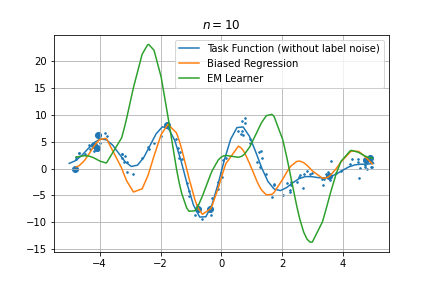
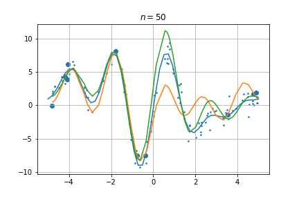
Figure 1: Examples of predictions on the synthetic, ‘Fourier’ meta-learning problem. Training data is shown in bold, small dots show test data. We also show the predictions for two learners (at every input) and the target function. The column correspond to outputs obtained training on $n\in\{10,50,100\}$ tasks. Our new algorithm, EM learner, performs quite well.

Our contributions.

In the present paper we revisit the framework underlying biased regularized regression. In particular, we propose to study the case when the unknown parameter vectors for the tasks are generated from a normal distribution with some mean and covariance matrix. First, we consider the case when the mean is unknown while the covariance matrix is known. For this case, in the context of fixed-design linear regression, we prove distribution-dependent lower and upper bounds, which essentially match each other. The lower bound is a direct lower limit on the transfer risk of any meta-learning method. The upper bound is proven for a version of a weighted biased regularized least-squares regression. Here, the parameters are biased towards the maximum likelihood estimate of the unknown common mean of the task parameter vectors, and the weighting is done with respect to the inverse covariance matrix of the distribution over the task parameter vectors. We show that the maximum likelihood estimator can be efficiently computed, which implies that the entire procedure is efficient. As opposed to the work of Tripuraneni et al. (2020), the gap between the lower and upper bounds is a universal constant, regardless of the other parameters of the meta-learning task. The matching lower and upper bounds together provide a precise and fine-grained characterization of the benefits of meta-learning. Our algorithm shows how one should combine datasets of different cardinalities and suggest specific ways of tuning biased regularized regression based on the noise characteristics of the data and the task structure. Our lower bounds are based on a rigorously proven novel observation, which may be of interest on its own. According to this observation, any predictor can be treated as a plug-in method that first estimates the unknown task distribution parameters. Hence, to prove a lower bound for the transfer risk, it suffices to do so for plug-in estimators.

In the last part of the paper we consider the case when the covariance matrix of the task parameter vector distribution is unknown. Importantly, this case can be seen as a way of unifying the representation learning stream of meta-learning with the parameter sharing stream. In particular, if the covariance matrix is such that $d-s$ of its eigenvalues tend to zero, while the other eigenvalues $s$ are allowed to take on arbitrarily large values, the problem becomes essentially the same as the representation learning problem of Du et al. (2020); Tripuraneni et al. (2020).

While we provide no theoretical analysis for this case, we give a detailed description of how the Expectation-Maximization (EM) algorithm can be used to tackle this problem. In particular, we show that in this special case the EM algorithm enjoys an efficient implementation: we show how to implement the iterative steps in the loop of the EM algorithm in an efficient way. The steps of this algorithm are given as closed-form expressions, which are both intuitive and straightforward to implement. We demonstrate the effectiveness of the resulting procedure on a number of synthetic and real benchmarks; Fig. 1 shows an example on a synthetic benchmark problem, comparing our EM algorithm with the earlier cited (unweighted) “biased regression” procedure. As can be seen from the figure, the EM based learner is significantly more effective. Further experiments suggest that the EM learner is almost as effective as the optimal biased weighted regularized regression procedure that is given the unknown parameters. We found that the EM learner is also competitive as a representation learning algorithm by comparing it to the algorithm of Tripuraneni et al. (2020) that is based on the “method-of-moments” technique.

2 Setup

In the statistical approach to meta-learning (Baxter, 1998, 2000) the learner observes a sequence of training tuples $\mathcal{D}=(D_{i})_{i=1}^{n}$, distributed according to a random sequence of task distributions $(P_{i})_{i=1}^{n}$, i.e. $D_{i}\sim P_{i}$, and furthermore task distributions are sampled independently from each other from a fixed and unknown environment distribution $\mathcal{P}$. The focus of this paper is linear regression with a fixed design and therefore each training tuple $D_{i}=\big{(}(\bm{x}_{i,1},Y_{i,1}),\ldots,(\bm{x}_{i,m_{i}},Y_{i,m_{i}})\big{)}$ consists of $m_{i}$ fixed training inputs from $\mathbb{R}^{d}$ and corresponding random, real-valued targets satisfying

$$Y_{i,j}=\bm{\theta}_{i}^{\top}\bm{x}_{i,j}+\varepsilon_{i,j},$$ (1)

where $$\varepsilon_{i,j}\mathbin{\overset{\mathrm{iid}}{\sim}}\mathcal{N}(0,\sigma^{2}),\ \bm{\theta}_{i}\mathbin{\overset{\mathrm{iid}}{\sim}}\mathcal{N}(\bm{\alpha},\bm{\Sigma})\,,$$

while $(\varepsilon_{i,j})_{i,j}$ and $(\bm{\theta}_{i})_{i}$ are also independent from each other. A meta-learning environment in this setting is thus given by $\bm{\alpha}$ and the noise parameters $(\sigma^{2},\bm{\Sigma})$. Initially, we will assume that $(\sigma^{2},\bm{\Sigma})$ is known, while $\bm{\alpha}$ (just like $(\bm{\theta}_{i})_{i}$) is unknown. The learner observes $\mathcal{D}$ and needs to produce a prediction of the value

$$Y=\bm{\theta}_{n}^{\top}\bm{x}+\varepsilon~{}$$

where $\varepsilon\sim\mathcal{N}(0,\sigma^{2})$ and where $\bm{x}\in\mathbb{R}^{d}$ is a fixed (non-random) point. Our theoretical results will trivially extend to the case when the learner needs to produce predictions for a sequence of input points or a fixed distribution over these, as often considered in meta-learning literature (Denevi et al., 2018; Du et al., 2020). The (random) transfer risk of the learner is defined as

$$\mathcal{L}(\bm{x}) =\mathbb{E}\left[(Y-\hat{Y})^{2}\;\middle|\;\mathcal{D}\right]\,.$$

The setting described above coincides with the standard fixed-design linear regression setup for $n=1$ and $\bm{\Sigma}\to\bm{0}$, for which the behavior of risk is well understood. In contrast, the question that meta-learning poses is whether having $n>1$, one can design a predictor that achieves lower risk compared to the approach that only uses the target data. Naturally, this is of a particular interest in the small sample regime when for all tasks, $m_{i}\ll n$, that is when facing scarcity of the training data but having many tasks. Broadly speaking, this reduces to understanding the behavior of the risk in terms of the interaction between the number of tasks $n$, their sample sizes $(m_{1},\ldots,m_{n})$, and the task structure given by the noise parametrization $(\sigma^{2},\bm{\Sigma})$.

3 Sufficiency of Meta-mean Prediction

In this section we show that there is no loss of generality in considering “plug-in” predictors that predict first the unknown meta-mean $\bm{\alpha}$. We also show that biased regularized least-squares estimator belongs to this family. We start with some general remarks and notation.

Throughout the rest of the paper, for real symmetric matrices $\bm{A}$ and $\bm{B}$, we use $\bm{A}\succeq\bm{B}$ to indicate that the matrix $\bm{A}-\bm{B}$ is Positive Semi-Definite (PSD). For $\bm{x}\in\mathbb{R}^{d}$ and PSD matrix $\bm{A}$, we let $\|\bm{x}\|_{\bm{A}}=\sqrt{\bm{x}^{\top}\bm{A}\bm{x}}$. We use $\|\bm{x}\|$ to denote the $2$-norm of $\bm{x}$. In the following we will use matrix notation aggregating inputs, targets, and parameters over multiple tasks. In particular, let the cumulative sample size of all tasks be $M=m_{1}+\dots+m_{n}$ and introduce aggregates for inputs and targets as follows:

$$\bm{X}_{i}=\underbrace{\begin{bmatrix}\bm{x}_{i,1}^{\top}\\ \vdots\\ \bm{x}_{i,m_{i}}^{\top}\end{bmatrix}}_{m_{i}\times d},\bm{\Psi}=\underbrace{\begin{bmatrix}\bm{X}_{1}\\ \vdots\\ \bm{X}_{n}\end{bmatrix}}_{M\times d},\bm{Y}_{i}=\underbrace{\begin{bmatrix}Y_{i,1}\\ \vdots\\ Y_{i,m_{i}}\end{bmatrix}}_{m_{i}\times 1},\bm{Y}=\underbrace{\begin{bmatrix}\bm{Y}_{1}\\ \vdots\\ \bm{Y}_{n}\end{bmatrix}}_{M\times 1}$$

$$\bm{X}=\underbrace{\begin{bmatrix}\bm{X}_{1}&\dots&\bm{0}\\ \vdots&\ddots&\vdots\\ \bm{0}&\dots&\bm{X}_{n}\end{bmatrix}}_{M\times nd},\quad\bm{\Theta}=\underbrace{\begin{bmatrix}\bm{\theta}_{1}\\ \vdots\\ \bm{\theta}_{n}\end{bmatrix}}_{nd\times 1}~{}.$$

The matrix representation allows us to compactly state the regression model simultaneously over all tasks. In particular, for the $M$-dimensional noise vector $\bm{\varepsilon}\sim\mathcal{N}(\bm{0},\sigma^{2}\bm{I})$:

$$\bm{Y}=\bm{X}\bm{\Theta}+\bm{\varepsilon}\quad\Leftrightarrow\quad\bm{Y}\sim\mathcal{N}(\bm{\Psi}\bm{\alpha},\bm{K})$$ (2)

where $\bm{\alpha}$ is a meta-mean of model (1) and $\bm{K}$ is the marginal covariance matrix defined as $\bm{K}=\bm{X}(\bm{I}\otimes\bm{\Sigma})\bm{X}^{\top}+\sigma^{2}\bm{I}$ where $\otimes$ stands for the Kronecker product. Note that the above equivalence comes from a straightforward observation that a linear map $\bm{\mathbf{X}}_{i}$ applied to the Gaussian r.v. $\bm{\theta}_{i}$ is itself Gaussian with mean $\mathbb{E}[\bm{Y}_{i}]=\bm{X}_{i}\mathbb{E}[\bm{\theta}_{i}]=\bm{X}_{i}\bm{\alpha}$ and covariance $\bm{X}_{i}\bm{\Sigma}\bm{X}_{i}^{T}+\sigma^{2}\bm{\mathbf{I}}$ which follows from the property that for any random vector $\bm{\xi}$ with covariance matrix $\bm{C}$, and matrix $\bm{A}$ of appropriate dimensions, covariance matrix of $\bm{A}\bm{\xi}$ is $\bm{A}\bm{C}\bm{A}^{\top}$, ultimately giving Eq. 2.

3.1 Plug-In Predictors and their Sufficiency

Both our lower and upper bounds will be derived from analyzing a family of “plug-in” predictors that aim to estimate $\bm{\theta}_{n}$ through estimating $\bm{\alpha}$. As we shall see, weighted biased regularization is also member of this family.

The said family is motivated by applying the well-known bias-variance decomposition to the risk of an arbitrary predictor $A:\operatorname{\text{supp}}(P_{1})\times\dots\times\operatorname{\text{supp}}(P_{n})\times\mathbb{R}^{d}\to\mathbb{R}$. Namely,

$$\mathcal{L}(\bm{x}) =\mathbb{E}\left[(Y-A(\mathcal{D},\bm{x}))^{2}\;\middle|\;\mathcal{D}\right]$$

$$=\mathbb{E}\left[\left(\mathbb{E}[Y\,|\,\mathcal{D}]-A(\mathcal{D},\bm{x})\right)^{2}+\mathbb{V}[Y\,|\,\mathcal{D}]\;\middle|\;\mathcal{D}\right]$$

where we used the law of total expectation and the fact that for any r.v. $\xi$, $\mathbb{E}[\xi^{2}]=\mathbb{E}[\xi]^{2}+\mathbb{V}[\xi]$. Since the variance term does not depend on $A$, it follows that the prediction problem reduces to predicting the posterior mean $\mathbb{E}[Y\,|\,\mathcal{D}]$, which, in our setting, can be given in closed form:

Proposition 3.1.

Let $Y=\bm{\theta}_{n}^{\top}\bm{x}+\varepsilon$ for $\varepsilon\sim\mathcal{N}(0,\sigma^{2})$ and some $\bm{x}\in\mathbb{R}^{d}$. Then,

$$\mathbb{E}[Y\,|\,\mathcal{D}] =\bm{x}^{\top}\bm{\mathcal{T}}\left(\bm{\Sigma}^{-1}\bm{\alpha}+\frac{1}{\sigma^{2}}\bm{X}_{n}^{\top}\bm{Y}_{n}\right)$$

$$\text{where}\quad\bm{\mathcal{T}} =\left(\bm{\Sigma}^{-1}+\frac{1}{\sigma^{2}}\bm{X}_{n}^{\top}\bm{X}_{n}\right)^{-1}~{}.$$

Proof.

See Appendix A. ∎

Since the only unknown parameter here is the meta-mean $\bm{\alpha}$, we expect that good predictors will just estimate the meta-mean and use the above formula. That is, these predictors take the form $(\mathcal{D},\bm{x})\mapsto\bm{x}^{\top}\hat{\bm{\theta}}_{n}(\bm{\alpha}(\mathcal{D},\bm{x}))$, where

$$\hat{\bm{\theta}}_{n}(\bm{a}) =\bm{\mathcal{T}}\left(\bm{\Sigma}^{-1}\bm{a}+\frac{1}{\sigma^{2}}\bm{X}_{n}^{\top}\bm{Y}_{n}\right)\quad\bm{a}\in\mathbb{R}^{d}~{},$$ (3)

giving our family of plug-in predictors. In fact, there is no loss in generality by considering only predictors of the above form. Indeed, given some predictor $A$ and $\bm{x}\neq\bm{\mathbf{0}}$, we can solve $A(\mathcal{D},\bm{x})=\bm{x}^{\top}\hat{\bm{\theta}}_{n}(\bm{\alpha})$ for $\bm{\alpha}$. One solution is given by $\bm{\alpha}(\mathcal{D},\bm{x})=\bm{\Sigma}\bm{\mathcal{T}}^{-1}\bm{x}c$ where $c=\tfrac{1}{\|\bm{x}\|^{2}}\left(A(\mathcal{D},\bm{x})-\sigma^{-2}\bm{x}^{\top}\bm{\mathcal{T}}\bm{X}_{n}^{\top}\bm{Y}_{n}\right)$. Hence, to prove a lower bound for any regressor $A$, it will be enough to prove it for algorithms that estimate $\bm{\alpha}$.

One special estimator of $\bm{\alpha}$ is the Maximum Likelihood Estimator (MLE) estimator, and, thanks to (2), can be obtained via $\hat{\bm{\alpha}}^{\text{{mle}}}=\operatorname*{arg\ max}_{\bm{a}\in\mathbb{R}^{d}}\ln p^{\text{{g}}}(\bm{Y};\bm{\Psi}\bm{a},\bm{K})$, where $p^{\text{{g}}}(\bm{x};\bm{\mu},\bm{\Sigma})\propto e^{-\tfrac{1}{2}\|\bm{x}-\bm{\mu}\|_{\bm{\Sigma}^{-1}}^{2}}$ is a Guassian PDF. Some standard calculations give us

$$\hat{\bm{\alpha}}^{\text{{mle}}}=(\bm{\Psi}^{\top}\bm{K}^{-1}\bm{\Psi})^{-1}\bm{\Psi}^{\top}\bm{K}^{-1}\bm{Y}~{}.$$ (4)

3.2 Weighted Biased Regularization

Biased regularization is a popular transfer learning technique which commonly appears in the regularized formulations of the empirical risk minimization problems, where one aims at minimizing the empirical risk (such as the mean squared error) while forcing the solution to stay close to some bias variable $\bm{b}$. Here we consider the Weighted Biased Regularized Least Squares (WBRLS) formulation defined w.r.t. bias $\bm{b}$ and some PSD matrix $\bm{\Gamma}$:

$$\hat{\bm{\theta}}_{n}^{\text{{wbrls}}}=\operatorname*{arg\ min}_{\bm{\theta}\in\mathbb{R}^{d}}\left\{\hat{\mathcal{L}}_{n}(\bm{\theta})+\frac{\lambda}{2}\|\bm{\theta}-\bm{b}\|_{\bm{\Gamma}}^{2}\right\}$$

where $$\hat{\mathcal{L}}_{n}(\bm{\theta})=\sum_{j=1}^{m_{n}}\left(Y_{n,j}-\bm{\theta}^{\top}\bm{x}_{n,j}\right)^{2}~{}.$$

Remarkably, an estimate $\hat{\bm{\theta}}_{n}^{\text{{wbrls}}}$ produced by WBRLS is equivalent to estimator $\hat{\bm{\theta}}_{n}(\hat{\bm{\alpha}})$ of Eq. 3 for the choice of $\bm{b}=\hat{\bm{\alpha}},\bm{\Gamma}=\bm{\Sigma}^{-1}$, and $\lambda=\sigma^{2}$. Thus, WBRLS is a special member of the family chosen in the previous section.

To see the equivalence, owing to the convenient least-squares formulation, we observe that

$$\hat{\bm{\theta}}_{n}^{\text{{wbrls}}}=\left(\bm{X}_{n}^{\top}\bm{X}_{n}+\lambda\bm{\Gamma}\right)^{-1}(\bm{X}_{n}^{\top}\bm{Y}_{n}+\lambda\bm{\Gamma}\bm{b})~{}$$

and from here the equivalence follows by substitution. A natural question commonly arising in such formulations is how to set the bias term $\bm{b}$. One choice can be $\bm{b}=\hat{\bm{\alpha}}^{\text{{mle}}}$ and in the following we will see that it is an optimal one.

4 Problem-Dependent Bounds

We now present our main results, which are essentially matching lower and upper bounds. The upper bounds concern the parameter estimator that uses the MLE estimate of $\bm{\alpha}$, while the lower bounds apply to any method. We also present a more precise lower bound that applies to estimators that are built on unbiased meta-mean estimators $\hat{\bm{\alpha}}$. As we shall see that plug-in predictors based on MLE will exactly match this lower bound. The general lower bounds are also quite precise: They differ from this lower bound only by a (relatively small) universal constant. We also give a high-probability variant of the same general lower bound.

Theorem 4.1.

Let $\bm{x}\in\mathbb{R}^{d}$ and consider the linear regression model (1). Let $\hat{\bm{\alpha}}$ be any unbiased estimator of $\bm{\alpha}$ based on $\mathcal{D}$. Then the transfer risk $\mathcal{L}(\bm{x})$ of the predictor that predicts $\hat{Y}=\bm{x}^{\top}\hat{\bm{\theta}}_{n}(\hat{\bm{\alpha}})$ satisfies

$$\mathbb{E}[\mathcal{L}(\bm{x})] \geq\bm{x}^{\top}\bm{M}\bm{x}+\bm{x}^{\top}\bm{\mathcal{T}}\bm{x}+\sigma^{2}$$ (5)

$$\text{where}\quad\bm{M} =\bm{\mathcal{T}}\bm{\Sigma}^{-1}(\bm{\Psi}^{\top}\bm{K}^{-1}\bm{\Psi})^{-1}\bm{\Sigma}^{-1}\bm{\mathcal{T}}~{}.$$

Moreover, for all predictors we have

$$\mathbb{E}[\mathcal{L}(\bm{x})]\geq\frac{\bm{x}^{\top}\bm{M}\bm{x}}{16\sqrt{e}}+\bm{x}^{\top}\bm{\mathcal{T}}\bm{x}+\sigma^{2}.$$ (6)

Finally, for any $\delta\in(0,1)$, with probability at least $1-\delta$ for all predictors we have

$$\mathcal{L}(\bm{x})\geq\frac{1}{2}\log\left(\frac{1}{4(1-\delta)}\right)\bm{x}^{\top}\bm{M}\bm{x}+\bm{x}^{\top}\bm{\mathcal{T}}\bm{x}+\sigma^{2}.$$

Proof.

The main ideas of the proof are in Section 4.2, while the complete proof is given in Appendix B. ∎

Note that the presented bounds are problem-dependent since they depend on a concrete task structure of the environment characterized by $(\bm{\Sigma},\sigma^{2})$. While the strength of the above bound is its generality, this generality makes the interpretation of the result challenging. We return to the interpretation of this result momentarily, after presenting results for the transfer risk for the plug-in method that uses the (unbiased) MLE meta-mean estimator $\hat{\bm{\alpha}}^{\text{{mle}}}$ defined in Eq. 4.

Theorem 4.2.

For the estimator $\hat{\bm{\theta}}_{n}(\hat{\bm{\alpha}}^{\text{{mle}}})$ and for any $\bm{x}\in\mathbb{R}^{d}$ we have

$$\mathbb{E}[\mathcal{L}(\bm{x})]=\bm{x}^{\top}\bm{M}\bm{x}+\bm{x}^{\top}\bm{\mathcal{T}}\bm{x}+\sigma^{2}\,.$$ (7)

Moreover for the same estimator, with probability at least $1-\delta,\delta\in(0,1)$ we have

$$\mathcal{L}(\bm{x})\leq 2\log\left(\frac{2}{\delta}\right)\bm{x}^{\top}\bm{M}\bm{x}+\bm{x}^{\top}\bm{\mathcal{T}}\bm{x}+\sigma^{2}.$$

Proof.

See Appendix C. ∎

Note that Eq. 7 is an equality for the transfer risk and it matches the lower bound available for unbiased estimators. This result, together with our lower bound shows that (i) the predictors based on $\hat{\bm{\alpha}}^{\text{{mle}}}$ is optimal, with matching constant within the set of predictors that is based on unbiased estimators of $\bm{\alpha}$. It also follows that (ii) apart from a constant factor of $16\sqrt{e}$ of the transfer risk, this predictor is also optimal among all predictors.

4.1 Interpretation of the Results

The following two corollaries specialize the lower bound of Theorem 4.1 in a way that will make the results more transparent. Note that while we give these simplified expressions for the lower bound (specifically, Eq. 6), these expressions also remain essentially true for the upper bound for the MLE estimator, since these differ only in minor details. The proofs of both corollaries are given in Appendix F.

Both specializations are concerned with the case when the inputs are isotropic, meaning that the input covariance matrix of task $i$ is $\frac{m_{i}}{d}\bm{I}$.

In the first result, in addition, we assume a spherical task structure: $\bm{\Sigma}=\tau^{2}\bm{I}$. Thus, the coordinates of the parameter vectors $\bm{\theta}_{i}$ are uncorrelated and share the same variance $\tau^{2}$.

Corollary 4.3.

Assume the same as in case of Eq. 6. In addition, let $\bm{\Sigma}=\tau^{2}\bm{I}$, suppose that $\bm{X}_{i}^{\top}\bm{X}_{i}=\frac{m_{i}}{d}\bm{I}$, and let $\|\bm{x}\|=1$. Then,

$$\frac{\mathbb{E}[\mathcal{L}(\bm{x})]-\sigma^{2}}{\sigma^{2}}\geq\frac{H_{\tau^{2}}}{16\sqrt{e}}\cdot\frac{d^{2}\sigma^{2}}{n\left(\tau^{2}m_{n}+d\sigma^{2}\right)^{2}}+\frac{d\tau^{2}}{\tau^{2}m_{n}+d\sigma^{2}}\,,$$

where $H_{z}$ is a harmonic mean of a sequence $(z+\tfrac{d\sigma^{2}}{m_{i}})_{i=1}^{n}$.

In the above bound the first term vanishes as more tasks are added ($n$ growing). On the other hand, to decrease the second term, $m_{n}$ needs to increase. In particular, as $n\to\infty$, we get

$$\frac{\mathbb{E}[\mathcal{L}(\bm{x})]-\sigma^{2}}{\sigma^{2}}\geq\left(\frac{m_{n}}{d}+\frac{\sigma^{2}}{\tau^{2}}\right)^{-1}$$ (8)

where $\frac{m_{n}}{d}+\frac{\sigma^{2}}{\tau^{2}}$ can be interpreted as an effective sample size. Thus, while having infinitely many previous tasks have the potential to reduce the loss, the size of this effect is fixed and is related to the noise variance ratios. If $\tau^{2}\to 0$, having infinitely many tasks will allow perfect prediction, but for any $\tau^{2}>0$, there is a limit on how much the data of previous tasks can help. Finally, for the case $n=1$ and $\tau^{2}=0$ we recover the standard lower bound for linear setting $\mathbb{E}[\mathcal{L}(\bm{x})]-\sigma^{2}=\Omega(d\sigma^{2}/m_{1})$.

Our next result is concerned with “representation learning”, which corresponds to the case when $\bm{\Sigma}$ is a low rank PSD matrix.

Corollary 4.4.

Let the inputs be isotropic as before and $\|\bm{x}\|=1$. Moreover, let $\bm{\Sigma}$ be a PSD matrix of rank $s\leq d$ with eigenvalues $\lambda_{1}\geq\ldots\geq\lambda_{s}>0$, and suppose that $\|\bm{x}\|_{\bm{P}_{s}^{\top}\bm{P}_{s}}^{2}=s/d$ where $\bm{P}_{s}=[\bm{u}_{1},\ldots,\bm{u}_{s}]^{\top}$ and $(\bm{u}_{j})_{j=1}^{s}$ are unit length eigenvectors of $\bm{\Sigma}$. Then,

$$\frac{\mathbb{E}[\mathcal{L}(\bm{x})]-\sigma^{2}}{\sigma^{2}}\geq\frac{H_{\lambda_{s}}}{16\sqrt{e}}\cdot\frac{sd\sigma^{2}}{n\left(\lambda_{1}m_{n}+d\sigma^{2}\right)^{2}}+\frac{s\lambda_{s}}{\lambda_{s}m_{n}+d\sigma^{2}}~{}.$$

Note that the first term on the right-hand side of the last display scales with $sd/n$, where $sd$ is the number of parameter in a matrix that would give the low-dimensional representation and the second term scales with $s/m_{n}$ for $m_{n}\gg d\sigma^{2}/\lambda_{s}$. Somewhat surprisingly (given that here $\bm{\Sigma}$ is known), these essentially match the upper bounds due to Du et al. (2020); Tripuraneni et al. (2020), implying that their results are unimprovable.

4.2 Proof Sketches

Our lower and upper bounds on the risk are based on an identity that holds for the transfer risk of plug-in methods. The identity is essentially a bias-variance decomposition.

Lemma 4.5.

For $\hat{\bm{\theta}}_{n}(\hat{\bm{\alpha}})$ defined in Eq. 3, any task mean estimator $\hat{\bm{\alpha}}$, and any $\bm{x}\in\mathbb{R}^{d}$ we have $\mathbb{E}[\mathcal{L}(\bm{x})]=\mathbb{E}\left[\left(\bm{x}^{\top}\bm{\mathcal{T}}\bm{\Sigma}^{-1}(\bm{\alpha}-\hat{\bm{\alpha}})\right)^{2}\right]+\bm{x}^{\top}\bm{\mathcal{T}}\bm{x}+\sigma^{2}.$

For the proof of this lemma we need the following proposition whose proof is given in Appendix A:

Proposition 4.6.

Let $Y=\bm{\theta}_{n}^{\top}\bm{x}+\varepsilon$ for $\varepsilon\sim\mathcal{N}(0,\sigma^{2})$ and some $\bm{x}\in\mathbb{R}^{d}$. Then, $\mathbb{E}[Y\,|\,\mathcal{D}]=\bm{x}^{\top}\bm{\mathcal{T}}\left(\bm{\Sigma}^{-1}\bm{\alpha}+\frac{1}{\sigma^{2}}\bm{X}_{n}^{\top}\bm{Y}_{n}\right)$ and $\mathbb{V}[Y\,|\,\mathcal{D}]=\bm{x}^{\top}\bm{\mathcal{T}}\bm{x}+\sigma^{2}$.

Proof of Lemma 4.5.

Using the law of total expectation and that for a r.v. $\xi$ we have $\mathbb{E}[\xi^{2}]=\mathbb{E}[\xi]^{2}+\mathbb{V}[\xi]$,

$$\mathcal{L}(\bm{x}) =\mathbb{E}\left[(Y-\hat{\bm{\theta}}_{n}(\hat{\bm{\alpha}})^{\top}\bm{x})^{2}\mid\mathcal{D}\right]$$

$$=\mathbb{E}\left[\left(\mathbb{E}[Y\,|\,\mathcal{D}]-\hat{\bm{\theta}}_{n}(\hat{\bm{\alpha}})^{\top}\bm{x}\right)^{2}+\mathbb{V}[Y\,|\,\mathcal{D}]\mid\mathcal{D}\right]$$

$$=\mathbb{E}\left[\left(\bm{x}^{\top}\bm{\mathcal{T}}\bm{\Sigma}^{-1}\left(\bm{\alpha}-\hat{\bm{\alpha}}\right)\right)^{2}\mid\mathcal{D}\right]+\bm{x}^{\top}\bm{\mathcal{T}}\bm{x}+\sigma^{2}\,,$$

where identities for $\mathbb{E}[Y\,|\,\mathcal{D}]$ and $\mathbb{V}[Y\,|\,\mathcal{D}]$ come from Proposition 4.6 and identity for $\hat{\bm{\theta}}_{n}(\hat{\bm{\alpha}})$ is due to (3). ∎

Thus, to establish universal lower bounds we need to lower bound $\mathbb{E}\left[\left(\bm{x}^{\top}\bm{\mathcal{T}}\bm{\Sigma}^{-1}(\bm{\alpha}-\hat{\bm{\alpha}})\right)^{2}\right]$ for any choice of estimator $\hat{\bm{\alpha}}$, which in combination with Lemma 4.5 will prove Theorem 4.1. Here, relying on the Cramér-Rao inequality (Theorem B.1), we only prove a lower bound for unbiased estimators, while the general case, whose proof uses Le Cam’s method, is left to Section B.2.

Lemma 4.7.

For any unbiased estimator $\hat{\bm{\alpha}}$ of $\bm{\alpha}$ in Eq. 2 we have $\mathbb{E}\left[\left(\bm{x}^{\top}\bm{\mathcal{T}}\bm{\Sigma}^{-1}(\bm{\alpha}-\hat{\bm{\alpha}})^{2}\right)\right]\geq\bm{x}^{\top}\bm{M}\bm{x}.$

Proof.

Recall that according to the equivalence (2), $\bm{Y}\sim\mathcal{N}(\bm{\Psi}\bm{\alpha},\bm{K})$ and the unknown parameter is $\bm{\alpha}$. To compute the Fisher information matrix we first observe that $\nabla_{\bm{\alpha}}\ln p^{\text{{g}}}\left(\bm{Y};\bm{\Psi}\bm{\alpha},\bm{K}\right)=\bm{\Psi}^{\top}\bm{K}^{-1}(\bm{Y}-\bm{\mathbf{\Psi\alpha}})$ and

$$\bm{F} =\mathbb{E}\left[\nabla_{\bm{\alpha}}\ln p^{\text{{g}}}\left(\bm{Y};\bm{\Psi}\bm{\alpha},\bm{K}\right)\nabla_{\bm{\alpha}}\ln p^{\text{{g}}}\left(\bm{Y};\bm{\Psi}\bm{\alpha},\bm{K}\right)^{\top}\right]$$

$$=\bm{\Psi}^{\top}\bm{K}^{-1}\mathbb{E}\left[(\bm{Y}-\bm{\Psi}\bm{\alpha})(\bm{Y}-\bm{\Psi}\bm{\alpha})^{\top}\right]\bm{K}^{-1}\bm{\Psi}$$

$$=\bm{\Psi}^{\top}\bm{K}^{-1}\bm{\mathbf{\Psi}}.$$

Thus, by the Cramér-Rao inequality we have $\mathbb{E}\left[(\bm{\alpha}-\hat{\bm{\alpha}})(\bm{\alpha}-\hat{\bm{\alpha}})^{\top}\right]\succeq(\bm{\Psi}^{\top}\bm{K}^{-1}\bm{\Psi})^{-1}~{}.$ Finally, left-multiplying by $\bm{x}^{\top}\bm{\mathcal{T}}\bm{\Sigma}^{-1}$ and right-multiplying the above by $\bm{\Sigma}^{-1}\bm{\mathcal{T}}\bm{x}$ gives us the statement. ∎

5 Learning with Unknown Task Structure

So far we have assumed that parameters $(\sigma^{2},\bm{\Sigma})$ characterizing the structure of environment are known, which limits the applicability of the predictor (though does not limit the lower bound). Staying within our framework, a natural idea is to estimate all the environment parameters $\mathcal{E}=(\bm{\alpha},\sigma^{2},\bm{\Sigma})$ by maximizing the data marginal log-likelihood

$$J(\mathcal{D},\mathcal{E}^{\prime})=\ln\int_{\mathbb{R}^{nd}}p(\mathcal{D}\,|\,\bm{\vartheta})\mathop{}\!\mathrm{d}p(\bm{\vartheta}\,|\,\mathcal{E}^{\prime})$$

over $\mathcal{E}^{\prime}$, where $p(\mathcal{D},\bm{\Theta},\mathcal{E})$ stands for the joint distribution in the model (1). The above problem is non-convex. As such, we propose to use EM procedure (Dempster et al., 1977), which is known to be a reasonable algorithm for similar settings. EM can be derived as a procedure that maximizes a lower bound on $J(\mathcal{D},\mathcal{E}^{\prime})$: Jensen’s inequality gives us that for any probability measure $q$ on $\mathbb{R}^{nd}$, $J(\mathcal{D},\mathcal{E}^{\prime})\geq\int\ln\left(\frac{p(\bm{\vartheta},\mathcal{D}\,|\,\mathcal{E}^{\prime})}{q(\bm{\vartheta})}\right)\mathop{}\!\mathrm{d}q(\bm{\vartheta})$. This is then maximized in $\mathcal{E}^{\prime}$ and $q$ in an alternating fashion: Letting $\hat{\mathcal{E}}_{t}$ to be a parameter estimate at step $t$, we maximize the lower bound in $q$ for a fixed $\mathcal{E}^{\prime}=\hat{\mathcal{E}}_{t}$, and then obtain $\hat{\mathcal{E}}_{t+1}$ by maximizing the lower bound in $\mathcal{E}^{\prime}$ for a fixed previously obtained solution in $q$. Maximization in $q$ gives us $q(\bm{\vartheta})=p(\bm{\vartheta}\,|\,\mathcal{D},\hat{\mathcal{E}}_{t})$, while maximization in $\mathcal{E}^{\prime}$ yields

$$\hat{\mathcal{E}}_{t+1}\in\operatorname*{arg\ max}_{\mathcal{E}^{\prime}}\int\ln\left(p(\bm{\vartheta},\mathcal{D}\,|\,\mathcal{E}^{\prime})\right)\mathop{}\!\mathrm{d}p(\bm{\vartheta}\,|\,\mathcal{D},\hat{\mathcal{E}}_{t})~{}.$$ (9)

After some calculations (cf. Appendix D), this gives Algorithm 1. During the E-step (lines 4-5), the algorithm computes the parameters of the posterior distribution $\mathcal{N}(\bm{\theta}_{i}\,|\,\hat{\bm{\mu}}_{t,i},\hat{\bm{\mathcal{T}}}_{t,i})$ relying on $\hat{\mathcal{E}}_{t}$, and during the M-step (lines 7–9) it estimates $\hat{\mathcal{E}}_{t+1}$ based on $(\hat{\bm{\mu}}_{t,i},\hat{\bm{\mathcal{T}}}_{t,i})$. We propose to detect convergence (not shown) by checking the relative difference between successive parameter values.

Algorithm 1 EM procedure to estimate $(\bm{\alpha},\sigma^{2},\bm{\Sigma})$

0:  Initial parameter estimates $\hat{\mathcal{E}}_{1}=(\hat{\bm{\alpha}}_{1},\hat{\sigma}_{1}^{2},\hat{\bm{\Sigma}}_{1})$

0:  Final parameter estimates $\hat{\mathcal{E}}_{t}=(\hat{\bm{\alpha}}_{t},\hat{\sigma}_{t}^{2},\hat{\bm{\Sigma}}_{t})$

1:  $\hat{\bm{\mathcal{T}}}_{1,i}\leftarrow\bm{0},\ \hat{\bm{\mu}}_{1,i}\leftarrow\bm{0}$  $i\in[n]$

2:  repeat

3:     for $i=1,\ldots,n$ do  $\triangleright$ E-step

4:        $\hat{\bm{\mathcal{T}}}_{t,i}\leftarrow\left(\hat{\bm{\Sigma}}_{t}^{-1}+\hat{\sigma}_{t}^{-2}\bm{X}_{i}^{\top}\bm{X}_{i}\right)^{-1}$

5:        $\hat{\bm{\mu}}_{t,i}\leftarrow\hat{\bm{\mathcal{T}}}_{t,i}\left(\hat{\bm{\Sigma}}_{t}^{-1}\hat{\bm{\alpha}}_{t}+\hat{\sigma}_{t}^{-2}\bm{X}_{i}^{\top}\bm{Y}_{i}\right)$

6:     end for

7:     $\hat{\bm{\alpha}}_{t}\leftarrow\frac{1}{n}\sum_{i=1}^{n}\hat{\bm{\mu}}_{t,i}$ $\triangleright$ M-step

8:     $\hat{\bm{\Sigma}}_{t}\leftarrow\frac{1}{n}\sum_{i=1}^{n}\left(\hat{\bm{\mathcal{T}}}_{t,i}+(\hat{\bm{\mu}}_{t,i}-\hat{\bm{\alpha}}_{t})(\hat{\bm{\mu}}_{t,i}-\hat{\bm{\alpha}}_{t})^{\top}\right)$

9:     $\hat{\sigma}^{2}_{t}\leftarrow\frac{1}{n}\sum_{i=1}^{n}\frac{1}{m_{i}}\left(\hat{\mathcal{L}}_{i}(\hat{\bm{\mu}}_{t,i})+\mathrm{tr}\left(\bm{X}_{i}\hat{\bm{\mathcal{T}}}_{t,i}\bm{X}_{i}^{\top}\right)\right)$

10:     $t\leftarrow t+1$

11:  until Convergence (see discussion)

6 Experiments

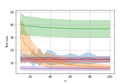
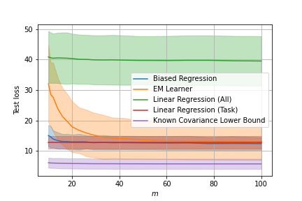
Figure 2: Test errors on Fourier synthetic experiment with changing number of tasks $n$ and number of samples per task $m$. When one of the parameters changes, the other one is set to 10.

In this section we present experiments designed to verify three hypotheses: (i) Under ideal circumstances, the predictor $\bm{x}^{\top}\hat{\bm{\theta}}_{n}(\hat{\bm{\alpha}}^{\text{{mle}}})$ is superior to its alternatives, including biased, but unweighted regression; (ii) The EM-algorithm reliably recovers unknown parameters of the environment and is also suitable for representation learning; (iii) our distribution-dependent lower bound Eq. 5 is numerically sharp. In addition, we briefly report on experiments with a real-world dataset.

Baselines.

We consider two non-meta-learning baselines, that is Linear Regression (All) — Ordinary Least Squares (OLS) fitted on $\mathcal{D}^{\backslash n}=(D_{i})_{i=1}^{n-1}$, which excludes the newly observed task, and Linear Regression (Task) — OLS fitted on a newly encountered task $D_{n}$. Next, we consider meta-learning algorithms. We report performance of the unweighted Biased Regression procedure with bias set to the least squares solution $(\sum_{i\neq n}\bm{X}_{i}^{\top}\bm{X}_{i})^{-1}\sum_{i\neq n}\bm{X}_{i}^{\top}\bm{Y}_{i}$ and $\lambda$ found by cross-validation (cf. Appendix E). Note that the bias and the regularization coefficient are found on $\mathcal{D}^{\backslash n}$, while $D_{n}$ is used for the final fitting. EM Learner is estimator (3) with all environment parameters found by Algorithm 1 on $\mathcal{D}^{\backslash n}$. The convergence threshold was set to $10^{-6}$ while the maximum number of iterations was set to $10^{3}$. Finally, we report numerical values of Eq. 5 as Known Covariance Lower Bound. For all of the experiments we show averages and standard deviations of the mean test errors computed over $30$ independent runs of that experiment.

Synthetic Experiments.

We conduct synthetic experiments on datasets with Fourier generated features and features sampled from a $d$-dimensional unit sphere. In all of the synthetic experiments we have $\bm{\mathbf{\alpha}}=\bm{\mathbf{0}},\sigma^{2}=1$ and $\bm{\mathbf{\Sigma}}$ generated by computing $\bm{\Sigma}=\bm{\mathbf{LL}}^{\top}+\eta\bm{I}$ where $L_{ij}=\mathbb{I}\left\{i\geq j\right\}Z_{ij}$ with $Z_{ij}$ and $\eta$ sampled from the standard normal distribution. Test error is computed on 100 test tasks using 10 examples for training and $100$ examples for testing.

For the Fourier-features, we sample a value $u\sim\mathcal{U}(-5,5)$ and compute features by evaluating $d=11$ Fourier basis functions at $u$: $x_{j}=\mathbb{I}\{1\leq j\leq 5\}\sin(\frac{j}{5}\pi u)+\mathbb{I}\{6\leq j\leq 10\}\cos(\frac{j-5}{5}\pi u)+\mathbb{I}\{j=11\}$, where $\mathbb{I}\{E\}=1$ if $E$ is true and $\mathbb{I}\{E\}=0$ otherwise. Examples of these tasks and results of meta-learning on some of these were shown in Fig. 1. In Fig. 2 we show the test errors for various meta-learners while varying the number of tasks $n$ and task sizes $m$. For the ‘spherical’ data, the same is shown in Fig. 3. Here, we generate $\bm{x}$ from a $d=42$ dimensional unit sphere. In both experiments for sufficiently large number of training tasks the EM-based learner approaches the optimal estimator even when the number of examples per task is less than the dimensionality of that task.

In the context of the ‘Fourier’ dataset, we also experimented with generating low-rank $\bm{\Sigma}$, corresponding to the challenge of learning a low-dimensional representation, shared across the tasks. We found that the EM-based meta learner stays competitive in this setting. To save space, the results are presented in Appendix G.

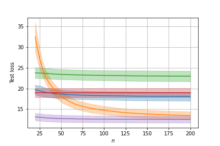
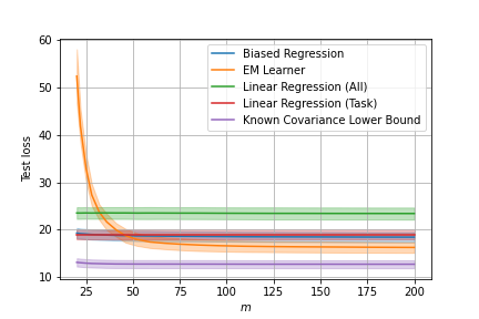
Figure 3: Test error on spherical synthetic experiment with changing number of tasks $n$ and number of samples per task $m$. When one of the parameters changes, the other one is set to 40.

Real Dataset Experiment.

We also conducted experiments on a real world dataset containing information about students in $139$ schools in years $1985$-$1987$ (Dua & Graff, 2017, School Dataset). We adapt the dataset to a meta-learning problem with the goal to predict the exam score of students based on the student-specific and school-specific features. After one-hot encoding of the categorical values there are $d=27$ features for each student. We randomly split schools into two subsets: The first, consisting of $100$ schools, forms $\mathcal{D}^{\backslash n}$ (used for training the bias, $\lambda$ selection, and EM). The second subset consists of $39$ schools, where each school is further split into $80\%/20\%$ for the final training and testing of the meta-learners. Results are given in Fig. 4. We can see that while both Biased Regression and EM Learner outperform regression, their performance is very similar. This could be attributed to the fact that the features mostly contain weakly relevant information, which is confirmed by inspecting the coefficient vector.

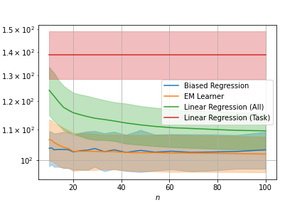
Figure 4: Test error on the School Dataset. Up to $100$ schools are used for fitting environment-related parameters (see text for details) and the remaining $39$ are used as the target task.

Representation learning experiments I.

Figure 5: Test error when the task covariance matrix is low-rank. As usual, on the left the number of tasks is changed, on the right, the number of training datapoints (per task). When one parameter is varied, the other is set to the value of $10$.

Our next figure (Fig. 5) shows the outcomes of experiments for the Fourier task but when $\bm{\Sigma}$ is low-rank. As can be seen, the EM based learner excels in exploiting the low-rank structure. For this experiment we have the same setup as for the Fourier experiment, but the covariance matrix $\bm{\Sigma}$ is generated by computing $\bm{\Sigma}=\bm{\mathbf{LL}}^{\top}$ where $\bm{\mathbf{L}}$ is a $d\times r$ matrix with $r=\lfloor d/2\rfloor=5$ and elements $L_{i,j}\sim\mathcal{N}(0,1)$. Note that in this case we can write $\bm{\theta}_{i}=\bm{\mathbf{B}}\bm{w}_{i}$ for some matrix $\bm{\mathbf{B}}$ of size $d\times r$ and vector $\bm{\mathbf{w}}_{i}$ of size $r$ sampled from multivariate normal distribution. Thus, if the matrix $\bm{\mathbf{B}}$ is known or estimated during training, one can project the features $\bm{x}_{i,j}$ onto a lower-dimensional space by computing $\bm{\mathbf{B}}^{\top}\bm{x}_{i,j}$ to speed up the adaptation to new tasks by running least-squares regression to estimate $\bm{w}_{i}$ instead of $\bm{\mathbf{\theta}}_{i}$.

In addition to the baselines described in the main text, we compared EM Learner with two additional baselines: one is based on the Method of Moments (MoM) estimator from Tripuraneni et al. (2020) (not shown on the figure), and another which we refer to as Oracle Representation. We omit displaying the error of the method of moments estimator since for the features generated as in this experiment it is not able to perform estimation of the subspace and leads to test errors with values around $60$. At the same time, as shown on Fig. 5 (left) we observe that EM Learner can outperform Oracle Representation which assumes the knowledge of the covariance matrix $\bm{\Sigma}$ from which it computes the subspace matrix $\bm{\mathbf{B}}$ and uses it to obtain lower-dimensional representation of the features when adapting to a new task via least-squares, as described above. This is possible because the coefficients estimated by EM are biased toward $\bm{\alpha}$ which does not happen with least squares regression in the lower dimensional subspace and this is beneficial, especially when the number of test-task training examples is small.

Representation learning experiments II.

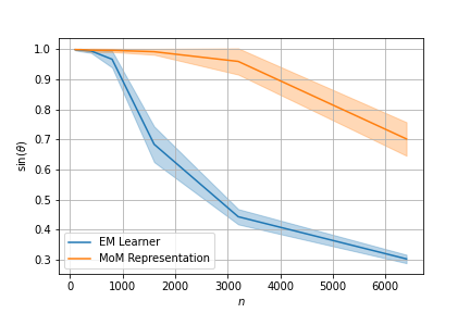
Figure 6: Max-correlation $d_{\max}(\bm{\hat{B}},\bm{B})$ between the estimated matrix $\bm{\hat{B}}$ (by the respective algorithm) and the ground truth matrix $\bm{B}$ while increasing number of tasks $n$.

To validate our implementation of the MoM estimator of Tripuraneni et al. (2020) and to investigate more whether EM is preferable to the MoM estimator beyond the setting that is ideal for the EM method we considered the experimental setup of Tripuraneni et al. (2020).

To explain the setup, we recall that the MoM estimator computes an estimate $\bm{\hat{B}}$ of the ground truth matrix $\bm{B}$. Tripuraneni et al. (2020) proves results for the max-correlation between $\bm{\hat{B}}$ and $\bm{B}$, and also reports experimentally measured max-correlation values between the ground truth and the MoM computed matrix. The max-correlation between matrices $\bm{A}$ and $\bm{A}^{\prime}$ is based on the definition of principal angles and is equal to $d_{\max}(\bm{A},\bm{A}^{\prime})=\sqrt{1-\cos^{2}(\bm{A},\bm{A}^{\prime})}$ where $\cos(\bm{A},\bm{A}^{\prime})=\max_{\bm{u}\in\operatorname{span}(\bm{A}):\|\bm{u}\|=1}\max_{\bm{v}\in\operatorname{span}(\bm{A}^{\prime}):\|\bm{v}\|=1}\bm{u}^{\top}\bm{v}$. Intuitively, max-correlation captures how well the subspaces spanned by matrices $\bm{A}$ and $\bm{A}^{\prime}$ are aligned.

To compare our EM estimator to MoM we run the EM estimator as described in Algorithm 1, and once the final estimate $\hat{\bm{\Sigma}}$ is obtained, we reduce its rank by clipping eigenvalues $\lambda_{s+1}\geq\ldots\geq\lambda_{d}$ to $0$.

We follow the experimental setup of Tripuraneni et al. (2020), that is, inputs are generated as $\bm{x}_{i}\sim\mathcal{N}(0,\bm{I}_{d})$, while the regression model is given by Eq. 1 with $(\sigma^{2},\bm{\Sigma})=(1,\tfrac{1}{s}\bm{B}\bm{B}^{\top})$. Here, columns of $\bm{B}\in\mathbb{R}^{d\times s}$ are sampled from a uniform distribution on a unit $d$-sphere. Finally, the number of examples per previously observed task is set as $m_{1}=...=m_{n-1}=5$, the representation rank is $s=5$, the input dimension is $d=100$, and the experiment is repeated $30$ times. Since we only estimate the subspace matrix we do not use the data from the test task $(\bm{X}_{n},\bm{y}_{n})$.

We report our results in Fig. 6, plotting the max-correlation between $\bm{\hat{B}}$ found by the respective algorithm and $\bm{B}$, while increasing the number of tasks. We see that EM learner considerably outperforms MoM Representation in terms of the subspace estimation to the degree captured by max-correlation. While we suspect that the improvement is due to the joint optimization over the covariance of environment and the mean of the environment (the bias in biased regularization), the detailed understanding of this effect is left for the future work.

7 Conclusions

While ours is the first work to derive matching, distribution-dependent lower and upper bounds, much works remains to be done: our approach to derive meta-learning algorithms based on a probabilistic model should be applicable more broadly and could lead to further interesting developments in meta-learning. The most interesting narrower question is to theoretically analyze the EM algorithm. Doing this in the low-rank setting looks particularly interesting. We hope that our paper will inspire other researchers to do further work in this area.

Appendix A Parameters of the Posterior Distribution

Recall that

$$p_{n}(\bm{\theta}_{n}\,|\,\mathcal{D})\propto p^{\text{{g}}}(\bm{Y}_{n}\,|\,\bm{X}_{n}\bm{\theta}_{n},\sigma^{2}\bm{I})p^{\text{{g}}}(\bm{\theta}_{n}\,|\,\bm{\alpha},\bm{\Sigma})~{}.$$

We first give a handy proposition for the posterior distribution over the parameters $\bm{\theta}_{n}$.

Proposition A.1.

$$\ln p_{n}(\bm{\theta}_{n})=-\frac{1}{2}(\bm{\theta}_{n}-\bm{\mu})\bm{\mathcal{T}}^{-1}(\bm{\theta}_{n}-\bm{\mu})+\mathrm{const}(\bm{\theta}_{n})$$

where covariance is

$$\bm{\mathcal{T}}=\left(\bm{\Sigma}^{-1}+\frac{1}{\sigma^{2}}\bm{X}_{n}^{\top}\bm{X}_{n}\right)^{-1}$$

and mean is

$$\bm{\mu}=\bm{\mathcal{T}}\left(\bm{\Sigma}^{-1}\bm{\alpha}+\frac{1}{\sigma^{2}}\bm{X}_{n}^{\top}\bm{Y}_{n}\right)~{}.$$

Proof.

The log-likelihood is the following chain of identities:

$$\ln p_{n}(\bm{\theta}_{n}) =-\frac{\sum_{j=1}^{m_{n}}(\bm{x}_{n,j}^{\top}\bm{\mathbf{\theta}}_{n}-Y_{n,j})^{2}}{2\sigma^{2}}-\frac{1}{2}(\bm{\theta}_{n}-\bm{\alpha})^{\top}\bm{\Sigma}^{-1}(\bm{\theta}_{n}-\bm{\alpha})+\mathrm{const}(\bm{\theta}_{n})$$

$$=-\frac{\sum_{j=1}^{m_{n}}(\bm{\theta}_{n}^{\top}\bm{x}_{n,j}\bm{x}_{n,j}^{\top}\bm{\theta}_{n}-2Y_{n,j}\bm{x}_{n,j}^{\top}\bm{\mathbf{\theta}}_{n})}{2\sigma^{2}}$$

$$=-\frac{1}{2}(\bm{\theta}_{n}^{\top}\bm{\Sigma}^{-1}\bm{\theta}_{n}-2\bm{\alpha}^{\top}\bm{\Sigma}^{-1}\bm{\theta}_{n})+\mathrm{const}(\bm{\theta}_{n})$$

$$=-\frac{1}{2}\left(\bm{\theta}_{n}^{\top}\bm{\mathcal{T}}^{-1}\bm{\theta}_{n}-2\left(\bm{\Sigma}^{-1}\bm{\alpha}+\frac{1}{\sigma^{2}}\bm{X}_{n}^{\top}\bm{Y}_{n}\right)^{\top}\bm{\theta}_{n}\right)+\mathrm{const}(\bm{\theta}_{n})$$

$$=-\frac{1}{2}(\bm{\theta}_{n}-\bm{\mu})\bm{\mathcal{T}}^{-1}(\bm{\theta}_{n}-\bm{\mu})+\mathrm{const}(\bm{\theta}_{n})~{}.$$

∎

First note that the first consequence of Proposition A.1 is a MLE for $\bm{\theta}_{n}$,

$$\hat{\bm{\theta}}_{n}^{\text{{mle}}}=\bm{\mathcal{T}}\left(\bm{\Sigma}^{-1}\bm{\alpha}+\frac{1}{\sigma^{2}}\bm{X}_{n}^{\top}\bm{Y}_{n}\right)~{}.$$

The second consequence is the following corollary which is obtained by taking $Y=\bm{\theta}_{n}^{\top}\bm{x}+\varepsilon$ and simply observing that the mean of a $p_{n}(\bm{\theta}_{n}\,|\,\mathcal{D})$ is $\bm{\mu}$, and so $\mathbb{E}[Y\,|\,\mathcal{D}]=\bm{x}^{\top}\bm{\mu}$ while the variance is $\mathbb{V}[Y\,|\,\mathcal{D}]=\mathbb{E}[(\bm{x}^{\top}\bm{\theta}_{n}+\varepsilon)^{2}\,|\,\mathcal{D}]-\mathbb{E}[(\bm{x}^{\top}\bm{\theta}_{n}+\varepsilon)\,|\,\mathcal{D}]^{2}=\bm{x}^{\top}\bm{\mathcal{T}}\bm{x}+\sigma^{2}$.

Proposition 4.6 (restated).

Let $Y=\bm{\theta}_{n}^{\top}\bm{x}+\varepsilon$ for $\varepsilon\sim\mathcal{N}(0,\sigma^{2})$ and some $\bm{x}\in\mathbb{R}^{d}$. Then,

$$\mathbb{E}[Y\,|\,\mathcal{D}]=\bm{x}^{\top}\bm{\mathcal{T}}\left(\bm{\Sigma}^{-1}\bm{\alpha}+\frac{1}{\sigma^{2}}\bm{X}_{n}^{\top}\bm{Y}_{n}\right)$$

and $$\mathbb{V}[Y\,|\,\mathcal{D}]=\bm{x}^{\top}\bm{\mathcal{T}}\bm{x}+\sigma^{2}~{}.$$

Appendix B Proof of the Lower Bounds

Our task reduces to establishing lower bounds on

$$\mathbb{E}\left[\left(\bm{x}^{\top}\bm{\mathcal{T}}\bm{\Sigma}^{-1}(\bm{\alpha}-\hat{\bm{\alpha}})\right)^{2}\right]$$ (10)

for any choice of estimator $\hat{\bm{\alpha}}$, which in combination with Lemma 4.5 will prove Theorem 4.1. In the next section we first prove a lower bound for any unbiased estimator relying on the Cramér-Rao inequality. In what follows, in Section B.2, we will show a general bound in Lemma B.4 valid for any estimator (possibly biased) using a hypothesis testing technique (see, e.g. (Lattimore & Szepesvári, 2018, Chap. 13)). Finally, in Lemma B.5 we prove a high-probability lower bound on Eq. 10.

B.1 Lower Bound for Unbiased Estimator $\hat{\bm{\alpha}}$

Theorem B.1 (Cramér-Rao inequality).

Suppose that $\bm{\alpha}\in\mathbb{R}^{d}$ is an unknown deterministic parameter with a probability density function $f(x\,|\,\bm{\alpha})$ and that $\hat{\bm{\alpha}}$ is an unbiased estimator of $\bm{\alpha}$. Moreover assume that for all $i,j\in[d]$, $x:f(x\,|\,\bm{\alpha})>0$, $\frac{\partial^{2}}{\partial\alpha_{i}\partial\alpha_{j}}\ln f(x\,|\,\bm{\alpha})$ exists and is finite, and $\frac{\partial^{2}}{\partial\alpha_{i}\partial\alpha_{j}}\int\hat{\bm{\alpha}}f(x\,|\,\bm{\alpha})\mathop{}\!\mathrm{d}x=\int\hat{\bm{\alpha}}\left(\frac{\partial^{2}}{\partial\alpha_{i}\partial\alpha_{j}}f(x\,|\,\bm{\alpha})\right)\mathop{}\!\mathrm{d}x$.

Then, for the Fisher information matrix defined as

$$\bm{F}=-\mathbb{E}\left[\nabla_{\bm{\alpha}}\ln f(X\,|\,\bm{\alpha})\nabla_{\bm{\alpha}}\ln f(X\,|\,\bm{\alpha})^{\top}\right]$$

we have

$$\mathbb{E}\left[(\hat{\bm{\alpha}}-\mathbb{E}[\hat{\bm{\alpha}}])(\hat{\bm{\alpha}}-\mathbb{E}[\hat{\bm{\alpha}}])^{\top}\right]\succeq\bm{F}^{-1}~{}.$$

Lemma B.2.

For any unbiased estimator $\hat{\bm{\alpha}}$ of $\bm{\alpha}$ in Eq. 2 we have

$$\mathbb{E}\left[\left(\bm{x}^{\top}\bm{\mathcal{T}}\bm{\Sigma}^{-1}(\bm{\alpha}-\hat{\bm{\alpha}})^{2}\right)\right]\geq\bm{x}^{\top}\bm{\mathcal{T}}\bm{\Sigma}^{-1}(\bm{\Psi}^{\top}\bm{K}\bm{\Psi})^{-1}\bm{\Sigma}^{-1}\bm{\mathcal{T}}\bm{x}.$$ (11)

Proof.

Recall that according to the equivalence (2) $\bm{Y}\sim\mathcal{N}(\bm{\Psi}\bm{\alpha},\bm{K})$ and the unknown parameter is $\bm{\alpha}$. To compute the Fisher information matrix we first observe that

$$\nabla_{\bm{\alpha}}\ln p^{\text{{g}}}\left(\bm{Y};\bm{\Psi}\bm{\alpha},\bm{K}\right)=\bm{\Psi}^{\top}\bm{K}^{-1}(\bm{Y}-\bm{\mathbf{\Psi\alpha}})$$

and so

$$\bm{F} =\mathbb{E}\left[\nabla_{\bm{\alpha}}\ln p^{\text{{g}}}\left(\bm{Y};\bm{\Psi}\bm{\alpha},\bm{K}\right)\nabla_{\bm{\alpha}}\ln p^{\text{{g}}}\left(\bm{Y};\bm{\Psi}\bm{\alpha},\bm{K}\right)^{\top}\right]$$

$$=\bm{\Psi}^{\top}\bm{K}^{-1}\mathbb{E}\left[(\bm{Y}-\bm{\Psi}\bm{\alpha})(\bm{Y}-\bm{\Psi}\bm{\alpha})^{\top}\right]\bm{K}^{-1}\bm{\Psi}$$

$$=\bm{\Psi}^{\top}\bm{K}^{-1}\bm{\mathbf{\Psi}}.$$

Thus, by Theorem B.1 we have

$$\mathbb{E}\left[(\bm{\alpha}-\hat{\bm{\alpha}})(\bm{\alpha}-\hat{\bm{\alpha}})^{\top}\right]\succeq(\bm{\Psi}^{\top}\bm{K}^{-1}\bm{\Psi})^{-1}~{}.$$

Finally, left-multiplying by $\bm{x}^{\top}\bm{\mathcal{T}}\bm{\Sigma}^{-1}$ and right-multiplying the above by $\bm{\Sigma}^{-1}\bm{\mathcal{T}}\bm{x}$ gives us the statement. ∎

B.2 Lower Bound for Any Estimator $\hat{\bm{\alpha}}$

The proof of is based on the following lemma.

Lemma B.3 (Bretagnolle & Huber 1979).

Let $P$ and $Q$ be probability measures on the same measurable

space $(\Omega,\mathcal{F})$, and let $A\in\mathcal{F}$ be an arbitrary event. Then,

$$P(A)+Q(A^{c})\geq\frac{1}{2}\exp(-\mathrm{D}_{\mathrm{KL}}(P,Q)),$$ (12)

where $\mathrm{D}_{\mathrm{KL}}(P,Q)=\int_{\Omega}\ln\left(P(\omega)/Q(\omega)\right)\mathop{}\!\mathrm{d}P(\omega)$ denotes Kullback-Leibler divergence between $P$ and $Q$ and $A^{c}=\Omega\setminus A$ is the complement of $A$.

Lemma B.4.

For any estimator $\hat{\bm{\alpha}}$ of $\bm{\alpha}$ in Eq. 2 we have

$$\mathbb{E}\left[\left(\bm{x}^{\top}\bm{\mathcal{T}}\bm{\Sigma}^{-1}(\hat{\bm{\alpha}}-\bm{\alpha})\right)^{2}\right]\geq\frac{\bm{x}^{\top}\bm{M}\bm{x}}{16\sqrt{e}}~{}.$$

Proof.

Throughout the proof let $\bm{q}=\bm{\Sigma}^{-1}\bm{\mathcal{T}}\bm{x}$. Consider two meta-learning problems with target distributions ${\mathbb{P}}$ and ${\mathbb{Q}}$ characterized by two means: $\bm{\alpha}_{{\mathbb{P}}}=\bm{0}$ and $\bm{\alpha}_{{\mathbb{Q}}}=\Delta(\bm{\Psi}^{\top}\bm{K}^{-1}\bm{\Psi})^{-1}\bm{q}$ where $\Delta>0$ is a free parameter to be tuned later on. Thus, according to our established equivalence (2), in these two cases targets are generated by respective models ${\mathbb{P}}=\mathcal{N}(\bm{0},\bm{K})$ and ${\mathbb{Q}}=\mathcal{N}(\Delta\bm{\Psi}(\bm{\Psi}^{\top}\bm{K}^{-1}\bm{\Psi})^{-1}\bm{q},\bm{K})$.

Recall our abbreviation $\bm{M}=\bm{\mathcal{T}}\bm{\Sigma}^{-1}(\bm{\Psi}^{\top}\bm{K}^{-1}\bm{\Psi})^{-1}\bm{\Sigma}^{-1}\bm{\mathcal{T}}$. Markov’s inequality gives

$$\mathbb{E}_{{\mathbb{P}}}\left[(\hat{\bm{\alpha}}^{\top}\bm{q}-\bm{\alpha}_{{\mathbb{P}}}^{\top}\bm{q})^{2}\right] =\mathbb{E}_{{\mathbb{P}}}\left[(\hat{\bm{\alpha}}^{\top}\bm{q})^{2}\right]\geq\frac{\Delta^{2}}{4}\left(\bm{x}^{\top}\bm{M}\bm{x}\right)^{2}{\mathbb{P}}\left(|\hat{\bm{\alpha}}^{\top}\bm{q}|\geq\frac{\Delta}{2}\bm{x}^{\top}\bm{M}\bm{x}\right)\,,\qquad\text{while}$$

$$\mathbb{E}_{{\mathbb{Q}}}\left[(\hat{\bm{\alpha}}^{\top}\bm{q}-\bm{\alpha}_{{\mathbb{Q}}}^{\top}\bm{q})^{2}\right] \geq\frac{\Delta^{2}}{4}\left(\bm{x}^{\top}\bm{M}\bm{x}\right)^{2}{\mathbb{Q}}\left(|\bm{\alpha}_{{\mathbb{Q}}}^{\top}\bm{q}-\hat{\bm{\alpha}}^{\top}\bm{q}|\geq\frac{\Delta}{2}\bm{x}^{\top}\bm{M}\bm{x}\right)$$

$$\geq\frac{\Delta^{2}}{4}\left(\bm{x}^{\top}\bm{M}\bm{x}\right)^{2}{\mathbb{Q}}\left(|\hat{\bm{\alpha}}^{\top}\bm{q}|<\frac{\Delta}{2}\bm{x}^{\top}\bm{M}\bm{x}\right)\,,$$

where the last inequality comes using the fact that $|a-b|\geq|a|-|b|$ for $a,b\in\mathbb{R}$ and observing that $\bm{\alpha}_{{\mathbb{Q}}}^{\top}\bm{q}=\bm{x}^{\top}\bm{M}\bm{x}$. Summing both inequalities above and applying Lemma B.3 we get

$$\mathbb{E}_{{\mathbb{P}}}\left[(\hat{\bm{\alpha}}^{\top}\bm{q}-\bm{\alpha}_{{\mathbb{P}}}^{\top}\bm{q})^{2}\right]+\mathbb{E}_{{\mathbb{Q}}}\left[(\hat{\bm{\alpha}}^{\top}\bm{q}-\bm{\alpha}_{{\mathbb{Q}}}^{\top}\bm{q})^{2}\right] \geq\frac{\Delta^{2}}{8}\left(\bm{x}^{\top}\bm{M}\bm{x}\right)^{2}\cdot\exp\left(-\mathrm{D}_{\mathrm{KL}}({\mathbb{P}},{\mathbb{Q}})\right)$$

$$\stackrel{{\scriptstyle(a)}}{{=}}\frac{\Delta^{2}}{8}\left(\bm{x}^{\top}\bm{M}\bm{x}\right)^{2}\cdot\exp\left(-\frac{\Delta^{2}}{2}\bm{x}^{\top}\bm{M}\bm{x}\right)\,,$$

where step $(a)$ follows from KL-divergence between multivariate Gaussians with the same covariance matrix. Now, using a basic fact that $2\max\left\{a,b\right\}\geq a+b$, we get that for any measure ${\mathbb{P}}$ given by parameter $\bm{\alpha}$ we have

$$\mathbb{E}\left[(\hat{\bm{\alpha}}^{\top}\bm{q}-\bm{\alpha}^{\top}\bm{q})^{2}\right]\geq\frac{\Delta^{2}}{16}\left(\bm{x}^{\top}\bm{M}\bm{x}\right)^{2}\cdot\exp\left(-\frac{\Delta^{2}}{2}\bm{x}^{\top}\bm{M}\bm{x}\right)~{}.$$

The statement then follows by choosing $\Delta^{2}=(\bm{x}^{\top}\bm{M}\bm{x})^{-1}$. ∎

Now we prove a high-probability version of the just given inequality.

Lemma B.5.

For any estimator $\hat{\bm{\alpha}}$ of $\bm{\alpha}$ in Eq. 2 and any $\delta\in(0,1)$ we have

$${\mathbb{P}}\left(\left(\bm{x}^{\top}\bm{\mathcal{T}}\bm{\Sigma}^{-1}(\hat{\bm{\alpha}}-\bm{\alpha})\right)^{2}\geq\ln\left(\frac{1}{4}\cdot\frac{1}{1-\delta}\right)\bm{x}^{\top}\bm{M}\bm{x}\right)\geq 1-\delta~{}.$$

Proof.

The proof is very similar to the proof of Lemma B.4 except we will not apply Markov’s inequality and focus directly on giving a lower bound the deviation probabilities rather than expectations. Thus, similarly as before introduce mean parameters $\bm{\alpha}_{{\mathbb{P}}}=\bm{0}$ and $\bm{\alpha}_{{\mathbb{Q}}}=\Delta(\bm{\Psi}^{\top}\bm{K}^{-1}\bm{\Psi})^{-1}\bm{q}/\left(\bm{x}^{\top}\bm{M}\bm{x}\right)$ and their associated probability measures ${\mathbb{P}}=\mathcal{N}(\bm{0},\bm{K})$ and ${\mathbb{Q}}=\mathcal{N}\left(\frac{\Delta\bm{\Psi}(\bm{\Psi}^{\top}\bm{K}^{-1}\bm{\Psi})^{-1}\bm{q}}{\bm{x}^{\top}\bm{M}\bm{x}},\bm{K}\right)$.

Note that

$${\mathbb{P}}\left(|\hat{\bm{\alpha}}^{\top}\bm{q}|\geq\frac{\Delta}{2}\right)={\mathbb{P}}\left(|\bm{\alpha}_{{\mathbb{P}}}^{\top}\bm{q}-\hat{\bm{\alpha}}^{\top}\bm{q}|\geq\frac{\Delta}{2}\right)~{},$$

$${\mathbb{Q}}\left(|\bm{\alpha}_{{\mathbb{Q}}}^{\top}\bm{q}-\hat{\bm{\alpha}}^{\top}\bm{q}|\geq\frac{\Delta}{2}\right)\geq{\mathbb{Q}}\left(|\hat{\bm{\alpha}}^{\top}\bm{q}|<\frac{\Delta}{2}\right)$$

and so by using Lemma B.3 we obtain an exponential tail bound

$${\mathbb{P}}\left(|\bm{\alpha}_{{\mathbb{P}}}^{\top}\bm{q}-\hat{\bm{\alpha}}^{\top}\bm{q}|\geq\frac{\Delta}{2}\right)+{\mathbb{Q}}\left(|\bm{\alpha}_{{\mathbb{Q}}}^{\top}\bm{q}-\hat{\bm{\alpha}}^{\top}\bm{q}|\geq\frac{\Delta}{2}\right)\geq\exp(-\mathrm{D}_{\mathrm{KL}}({\mathbb{P}}\,||\,{\mathbb{Q}}))=\frac{1}{2}\exp\left(-\frac{\Delta^{2}}{\bm{x}^{\top}\bm{M}\bm{x}}\right)~{}.$$

Setting the r.h.s. in the above to $2(1-\delta)$ where $\delta$ is an error probability, and solving for $\Delta$ gives us tuning

$$\Delta^{2}=2\ln\left(\frac{1}{4}\cdot\frac{1}{1-\delta}\right)\bm{x}^{\top}\bm{M}\bm{x}~{}.$$

Thus, we get

$${\mathbb{P}}\left(\left(\bm{\alpha}_{{\mathbb{P}}}^{\top}\bm{q}-\hat{\bm{\alpha}}^{\top}\bm{q}\right)^{2}\geq\ln\left(\frac{1}{4}\cdot\frac{1}{1-\delta}\right)\bm{x}^{\top}\bm{M}\bm{x}\right)+{\mathbb{Q}}\left(|\bm{\alpha}_{{\mathbb{Q}}}^{\top}\bm{q}-\hat{\bm{\alpha}}^{\top}\bm{q}|\geq\ln\left(\frac{1}{4}\cdot\frac{1}{1-\delta}\right)\bm{x}^{\top}\bm{M}\bm{x}\right)\geq 2(1-\delta)$$

and using the fact that $2\max(a,b)\geq a+b$ we get that for any probability measure ${\mathbb{P}}$ given by parameter $\bm{\alpha}$ we have

$${\mathbb{P}}\left(\left(\bm{\alpha}_{{\mathbb{P}}}^{\top}\bm{q}-\hat{\bm{\alpha}}^{\top}\bm{q}\right)^{2}\geq\ln\left(\frac{1}{4}\cdot\frac{1}{1-\delta}\right)\bm{x}^{\top}\bm{M}\bm{x}\right)\geq 1-\delta~{}.$$

∎

Appendix C Proof of the Upper Bounds

Theorem 4.2 (restated).

For the estimator $\hat{\bm{\theta}}_{n}(\hat{\bm{\alpha}}^{\text{{mle}}})$ and for any $\bm{x}\in\mathbb{R}^{d}$ we have

$$\mathbb{E}\left[\mathcal{L}(\bm{x})\right]=\bm{x}^{\top}\bm{M}\bm{x}+\bm{x}^{\top}\bm{\mathcal{T}}\bm{x}+\sigma^{2}.$$

Moreover for the same estimator, with probability at least $1-\delta,\delta\in(0,1)$ we have

$$\mathcal{L}(\bm{x})\leq 2\ln\left(\frac{2}{\delta}\right)\bm{x}^{\top}\bm{M}\bm{x}+\bm{x}^{\top}\bm{\mathcal{T}}\bm{x}+\sigma^{2}.$$

Proof.

Recall that

$$\hat{\bm{\alpha}}^{\text{{mle}}}=(\bm{\Psi}^{\top}\bm{K}^{-1}\bm{\Psi})^{-1}\bm{\Psi}^{\top}\bm{K}^{-1}\bm{Y}~{}.$$

The first result follows from Lemma 4.5 where we have to give an identity for

$$\mathbb{E}\left[\left(\bm{x}^{\top}\bm{\mathcal{T}}\bm{\Sigma}^{-1}(\bm{\alpha}-\hat{\bm{\alpha}}^{\text{{mle}}})\right)^{2}\right]$$ (13)

and the missing piece is a covariance of the estimator $\hat{\bm{\alpha}}^{\text{{mle}}}$

$$\mathbb{E}\left[(\bm{\alpha}-\hat{\bm{\alpha}}^{\text{{mle}}})(\bm{\alpha}-\hat{\bm{\alpha}}^{\text{{mle}}})^{\top}\right]$$

$$=(\bm{\Psi}^{\top}\bm{K}^{-1}\bm{\Psi})^{-1}\bm{\Psi}^{\top}\bm{K}^{-1}\mathrm{Cov}(\bm{Y},\bm{Y})\bm{K}^{-1}\bm{\Psi}(\bm{\Psi}^{\top}\bm{K}^{-1}\bm{\Psi})^{-1}$$

$$=(\bm{\Psi}^{\top}\bm{K}^{-1}\bm{\Psi})^{-1}~{}.$$ (14)

To prove the second result we have to give a high probability upper bound on Eq. 13.

Let $\bm{q}=\bm{\Sigma}^{-1}\bm{\mathcal{T}}\bm{x}$ and observe that $\bm{q}^{\top}\hat{\bm{\alpha}}^{\text{{mle}}}$ is Gaussian (since $\bm{Y}$ is composed of Gaussian entries) with mean $\bm{q}^{\top}\bm{\alpha}$ by equivalence (2), and covariance $(\bm{\Psi}^{\top}\bm{K}^{-1}\bm{\Psi})^{-1}$ by Eq. 14. Then, by Gaussian concentration for any error probability $\delta\in(0,1)$ we have

$${\mathbb{P}}\left((\bm{q}^{\top}\bm{\alpha}-\bm{q}^{\top}\hat{\bm{\alpha}}^{\text{{mle}}})^{2}\geq\sqrt{2\bm{q}^{\top}(\bm{\Psi}^{\top}\bm{K}^{-1}\bm{\Psi})^{-1}\bm{q}\ln\left(\frac{2}{\delta}\right)}\right)\leq\delta$$

which completes the proof. ∎

Appendix D Derivation of EM Steps

Recall that our goal is to solve

$$\max_{\mathcal{E}^{\prime}}\int\ln\left(p(\bm{\vartheta},\mathcal{D}\,|\,\mathcal{E}^{\prime})\right)\mathop{}\!\mathrm{d}p(\bm{\vartheta}\,|\,\mathcal{D},\hat{\mathcal{E}}_{t})~{}.$$

First, we will focus on the integral. The chain rule readily gives

$$\ln p(\bm{\Theta},\mathcal{D}\,|\,\mathcal{E}^{\prime})=\ln p(\bm{\Theta}\,|\,\mathcal{D},\mathcal{E}^{\prime})+\ln p(\bm{\Theta}\,|\,\mathcal{E}^{\prime})\,.$$

Using the same reasoning and notation as in the proof of Proposition A.1 we get

$$\int\ln p(\bm{\vartheta}\,|\,\mathcal{D},\mathcal{E}^{\prime})\mathop{}\!\mathrm{d}p(\bm{\vartheta}\,|\,\mathcal{D},\hat{\mathcal{E}}_{t}) =\sum_{i=1}^{n}\sum_{j=1}^{m_{i}}\left(\frac{1}{2}\ln\left(\frac{1}{\sigma^{2}}\right)-\frac{1}{2\sigma^{2}}\int(Y_{i,j}-\bm{x}_{i,j}^{\top}\bm{\vartheta}_{i})^{2}\mathop{}\!\mathrm{d}p(\bm{\vartheta}_{i}\,|\,\mathcal{D},\hat{\mathcal{E}}_{t})\right)+\mathrm{const}(\mathcal{E}^{\prime})$$

$$=\sum_{i=1}^{n}\sum_{j=1}^{m_{i}}\left(\frac{1}{2}\ln\left(\frac{1}{\sigma^{2}}\right)-\frac{1}{2\sigma^{2}}(Y_{i,j}-\bm{x}_{i,j}^{\top}\bm{\mu}_{i})^{2}-\bm{x}_{i,j}^{\top}\bm{\mathcal{T}}_{i}\bm{x}_{i,j}\right)+\mathrm{const}(\mathcal{E}^{\prime})\,,$$

using the fact that $\int(Y_{i,j}-\bm{x}_{i,j}^{\top}\bm{\vartheta}_{i})^{2}\mathop{}\!\mathrm{d}p(\bm{\vartheta}_{i}\,|\,\mathcal{D},\hat{\mathcal{E}}_{t})=(Y_{i,j}-\bm{x}_{i,j}^{\top}\bm{\mu}_{i})^{2}+\bm{x}_{i,j}^{\top}\bm{\mathcal{T}}_{i}\bm{x}_{i,j}$ where we took $\bm{\theta}_{i}\sim\mathcal{N}(\bm{\mu}_{i},\bm{\mathcal{T}}_{i})$ according to Proposition A.1.

Now we compute the expected log-likelihood of the vector of task parameters:

$$\int\ln p(\bm{\vartheta}\,|\,\mathcal{E}^{\prime})\mathop{}\!\mathrm{d}p(\bm{\vartheta}\,|\,\mathcal{D},\hat{\mathcal{E}}_{t})=\frac{n}{2}\ln\det\bm{\Sigma}^{-1}-\frac{1}{2}\sum_{i=1}^{n}\int(\bm{\vartheta}_{i}-\bm{\alpha})^{\top}\bm{\Sigma}^{-1}(\bm{\vartheta}_{i}-\bm{\alpha})\mathop{}\!\mathrm{d}p(\bm{\vartheta}_{i}\,|\,\mathcal{D},\hat{\mathcal{E}}_{t})+\mathrm{const}(\mathcal{E}^{\prime})~{}.$$

M-step for $\sigma^{2}$.

Now, note that since the likelihood of the vector of task variables $\bm{\Theta}$ does not depend on the parameter $\sigma^{2}$ we can solve for $\sigma^{2}$ based on the first order condition of the problem above. Differentiating the above equation with respect to $\sigma^{-2}$ (and ignoring the constant) gives

$$\sum_{i=1}^{n}\sum_{j=1}^{m_{i}}\left(\sigma^{2}-\left((Y_{i,j}-\bm{x}_{i,j}^{\top}\bm{\mu}_{i})^{2}+\bm{x}_{i,j}^{\top}\bm{\mathcal{T}}_{i}\bm{x}_{i,j}\right)\right).$$ (15)

while setting the derivative to zero gives

$$\sigma^{2}=\frac{1}{n}\sum_{i=1}^{n}\frac{1}{m_{i}}\sum_{j=1}^{m_{i}}\left((Y_{i,j}-\bm{x}_{i,j}^{\top}\bm{\mu}_{i})^{2}+\bm{x}_{i,j}^{\top}\bm{\mathcal{T}}_{i}\bm{x}_{i,j}\right).$$ (16)

M-step for $\bm{\alpha}$.

Differentiating the objective w.r.t. $\bm{\alpha}$ (and ignoring the constant) gives $\sum_{i=1}^{n}\bm{\Sigma}^{-1}(\mathbb{E}[\bm{\theta}_{i}]-\bm{\alpha})$ from which we get

$$\bm{\alpha}=\sum_{i=1}^{n}\bm{\mu}_{i}~{}.$$ (17)

M-step for $\bm{\Sigma}$.

Differentiating the expected log-likelihood of the vector of task parameters with respect to $\bm{A}=\bm{\Sigma}^{-1}$ gives

$$\sum_{i=1}^{n}\mathrm{tr}(\bm{\Sigma}d\bm{A})-\mathrm{tr}\int\left((\bm{\vartheta}_{i}-\bm{\alpha})(\bm{\vartheta}_{i}-\bm{\alpha})^{\top}d\bm{A}\right)\mathop{}\!\mathrm{d}p(\bm{\vartheta}_{i}\,|\,\mathcal{D},\hat{\mathcal{E}}_{t})$$ (18)

from which we get

$$\bm{\Sigma}=\frac{1}{n}\sum_{i=1}^{n}\mathbb{E}[(\bm{\theta}_{i}-\bm{\alpha})(\bm{\theta}_{i}-\bm{\alpha})^{\top}].$$ (19)

Finally, computing the expectation

$$\sum_{i=1}^{n}\left(\mathbb{E}[\bm{\theta}_{i}\bm{\theta}_{i}^{\top}]-2\bm{\mu}_{i}\bm{\alpha}^{\top}+\bm{\alpha}\bm{\alpha}^{\top}\right)=\sum_{i=1}^{n}\left((\bm{\mu}_{i}-\bm{\alpha})(\bm{\mu}_{i}-\bm{\alpha})^{\top}+\bm{\mathcal{T}}_{i}\right)$$ (20)

shows the update for $\bm{\Sigma}$.

Appendix E Selecting $\lambda$ in Biased Regression

The parameter $\lambda$ is selected via random search in the following way. For each of the 50 samples of $\lambda$ from log-uniform distribution on interval $[0;100]$ we perform the following procedure to estimate the risk $\hat{L}$. Firstly, we split the training tasks into $K=10$ groups $\mathcal{S}_{1},\dots,\mathcal{S}_{K}$ of (approximately) equal size and compute the estimates $\hat{\bm{\alpha}}_{k}$ using the data $\mathcal{S}^{\setminus k}$ from all of the groups excluding the group $k$: $\mathcal{S}^{\setminus k}:=\cup_{i\neq k}\mathcal{S}_{i}$. For each of the estimated values $\hat{\bm{\alpha}}_{k}$ we perform adaptation to and testing on the tasks in the group $\mathcal{S}_{k}$ using the given value of $\lambda$. We split the samples of each task data $D_{i}\in\mathcal{S}_{k}$ randomly into adaptation and test sets $10$ times each time such that the size of adaptation set is close to the size of adaptation sets used with the actual test data. For each of the splits we compute an estimate of the parameter vector $\hat{\bm{\theta}}_{k,i,l}$ where $k$ is the index of the group which was not used to estimate $\hat{\bm{\alpha}}_{k}$, $i$ is the index of a task data $D_{i}\in\mathcal{S}_{k}$, $l$ is the index of a random split of the samples in that task into adaptation and test sets. With this parameter vector and using the test set of the task $D_{i}\in\mathcal{S}_{k}$ we can also estimate the loss $\hat{L}_{k,i,l}$ after which all the loss values are averaged:

$$\hat{L}=\frac{1}{K}\sum_{k=1}^{K}\frac{1}{|\mathcal{S}^{\setminus k}|}\sum_{i:D_{i}\in\mathcal{S}^{\setminus k}}\frac{1}{10}\sum_{l=1}^{10}\hat{L}_{k,i,l}.$$

At the end we select the value of $\lambda$ which lead to the smallest value of $\hat{L}$ using this cross-validation procedure.

Appendix F Supplementary Statements

Proposition F.1.

For $\bm{M}$ (see Eq. 5) we have

$$\bm{M}=\sigma^{4}\cdot\left(\bm{\Sigma}\bm{X}_{n}^{\top}\bm{X}_{n}+\sigma^{2}\bm{I}\right)^{-1}\bm{A}^{-1}\left(\bm{\Sigma}\bm{X}_{n}^{\top}\bm{X}_{n}+\sigma^{2}\bm{I}\right)^{-1}\,,$$

where we denote

$$\bm{A}=\sum_{i=1}^{n}\bm{X}_{i}^{\top}(\bm{X}_{i}\bm{\Sigma}\bm{X}_{i}^{\top}+\sigma^{2}\bm{I})^{-1}\bm{X}_{i}~{}.$$

Proof.

Recall that

$$\bm{M}=\bm{\mathcal{T}}\bm{\Sigma}^{-1}\left(\bm{\Psi}^{\top}\bm{K}^{-1}\bm{\Psi}\right)^{-1}\bm{\Sigma}^{-1}\bm{\mathcal{T}}$$

and observe that

$$\bm{K}^{-1} =\begin{bmatrix}(\bm{X}_{1}\bm{\Sigma}\bm{X}_{1}^{\top}+\sigma^{2}\bm{I})^{-1}&\bm{0}&\dots&\bm{0}\\ \bm{0}&(\bm{X}_{2}\bm{\Sigma}\bm{X}_{2}^{\top}+\sigma^{2}\bm{I})^{-1}&\dots&\bm{0}\\ \vdots&&\ddots&\vdots\\ \bm{0}&\bm{0}&\dots&(\bm{X}_{n}\bm{\Sigma}\bm{X}_{n}^{\top}+\sigma^{2}\bm{I})^{-1}\end{bmatrix}\,,$$

which in turn implies

$$\bm{\Psi}^{\top}\bm{K}^{-1}\bm{\Psi}=\sum_{i=1}^{n}\bm{X}_{i}^{\top}(\bm{X}_{i}\bm{\Sigma}\bm{X}_{i}^{\top}+\sigma^{2}\bm{I})^{-1}\bm{X}_{i}~{}.$$

On the other hand,

$$\bm{\mathcal{T}}\bm{\Sigma}^{-1} =\left(\bm{\Sigma}^{-1}+\frac{1}{\sigma^{2}}\bm{X}_{n}^{\top}\bm{X}_{n}\right)^{-1}\bm{\Sigma}^{-1}$$

$$=\sigma^{2}\left(\sigma^{2}\bm{I}+\bm{\Sigma}\bm{X}_{n}^{\top}\bm{X}_{n}\right)^{-1}~{}.$$

Combining the above gives the statement. ∎

Lemma F.2.

In the following assume that $\bm{X}_{i}^{\top}\bm{X}_{i}=\frac{m_{i}}{d}\bm{I}$ for all $i.$ Let $\lambda_{j}(\bm{\Sigma})$ be the $j$th eigenvalue of $\bm{\Sigma}$. Then,

$$\lambda_{j}(\bm{M})=\sigma^{4}\cdot\frac{d^{2}}{\left(m_{n}\lambda_{j}(\bm{\Sigma})+d\sigma^{2}\right)^{2}}\cdot\frac{\text{HM}\left(\lambda_{j}(\bm{\Sigma})+\frac{d\sigma^{2}}{m_{i}}\right)_{i=1}^{n}}{n}\,,$$

where $\text{HM}(z_{i})_{i=1}^{n}$ denotes the harmonic mean of sequence $(z_{i})_{i=1}^{n}$. Moreover,

$$\lambda_{j}(\bm{\mathcal{T}})=\frac{d\sigma^{2}\lambda_{j}(\bm{\Sigma})}{d\sigma^{2}+m_{n}\lambda_{j}(\bm{\Sigma})}~{}.$$

Finally, the eigenvectors of $\bm{M}$ and $\bm{\mathcal{T}}$ coincide with the eigenvectors of $\bm{\Sigma}$.

Proof.

We first characterize eigenvalues of matrix $\bm{M}$. By Proposition F.1,

$$\bm{M}=\sigma^{4}\cdot\left(\bm{\Sigma}\bm{X}_{n}^{\top}\bm{X}_{n}+\sigma^{2}\bm{I}\right)^{-1}\bm{A}^{-1}\left(\bm{\Sigma}\bm{X}_{n}^{\top}\bm{X}_{n}+\sigma^{2}\bm{I}\right)^{-1}~{}.$$

We start with $\bm{A}^{-1}$, and by the spectral theorem, $\bm{\Sigma}=\bm{U}\bm{\Lambda}\bm{U}^{\top}$ for some unitary $\bm{U}$ and diagonal $\bm{\Lambda}$:

$$\bm{A}^{-1}=\left(\sum_{i=1}^{n}\bm{X}_{i}^{\top}(\bm{X}_{i}\bm{\Sigma}\bm{X}_{i}^{\top}+\sigma^{2}\bm{I})^{-1}\bm{X}_{i}\right)^{-1} =\left(\sum_{i=1}^{n}(\bm{\Sigma}\bm{X}_{i}^{\top}\bm{X}_{i}+\sigma^{2}\bm{I})^{-1}\bm{X}_{i}^{\top}\bm{X}_{i}\right)^{-1}$$

$$=\left(\sum_{i=1}^{n}\left(\bm{\Sigma}\cdot\frac{m_{i}}{d}+\sigma^{2}\bm{I}\right)^{-1}\frac{m_{i}}{d}\right)^{-1}$$

$$=\left(\sum_{i=1}^{n}\left(\bm{U}\bm{\Lambda}\bm{U}^{\top}\cdot\frac{m_{i}}{d}+\sigma^{2}\bm{I}\right)^{-1}\frac{m_{i}}{d}\right)^{-1}$$

$$=\bm{U}\left(\sum_{i=1}^{n}\left(\bm{\Lambda}+\frac{d\sigma^{2}}{m_{i}}\cdot\bm{I}\right)^{-1}\right)^{-1}\bm{U}^{\top}~{}.$$

Now,

$$\left(\bm{\Sigma}\bm{X}_{n}^{\top}\bm{X}_{n}+\sigma^{2}\bm{I}\right)^{-1} =\left(\bm{\Sigma}\cdot\frac{m_{n}}{d}+\sigma^{2}\bm{I}\right)^{-1}$$

$$=\left(\bm{U}\bm{\Lambda}\bm{U}^{\top}\cdot\frac{m_{n}}{d}+\sigma^{2}\bm{I}\right)^{-1}$$

$$=\bm{U}\left(\bm{\Lambda}\cdot\frac{m_{n}}{d}+\sigma^{2}\bm{I}\right)^{-1}\bm{U}^{\top}.$$

Thus,

$$\bm{M}=\bm{U}\left(\left(\bm{\Lambda}\cdot\frac{m_{n}}{d}+\sigma^{2}\bm{I}\right)^{2}\sum_{i=1}^{n}\left(\bm{\Lambda}+\frac{d\sigma^{2}}{m_{i}}\right)^{-1}\right)^{-1}\bm{U}^{\top}~{}.$$

and moreover the $j$th eigenvalue of $\bm{M}$ is

$$\lambda_{j}(\bm{M}) =\frac{1}{\left(\frac{m_{n}}{d}\lambda_{j}(\bm{\Sigma})+\sigma^{2}\right)^{2}}\cdot\frac{1}{\sum_{i=1}^{n}\frac{1}{\lambda_{j}(\bm{\Sigma})+\frac{d\sigma^{2}}{m_{i}}}}$$

$$=\frac{1}{\left(\frac{m_{n}}{d}\lambda_{j}(\bm{\Sigma})+\sigma^{2}\right)^{2}}\cdot\frac{\text{HM}\left(\lambda_{j}(\bm{\Sigma})+\frac{d\sigma^{2}}{m_{i}}\right)_{i=1}^{n}}{n}\,.$$

where recall that $\text{HM}(z_{i})_{i=1}^{n}$ denotes the harmonic mean of sequence $(z_{i})_{i=1}^{n}$.

Using the same arguments as above

$$\bm{\mathcal{T}} =\left(\bm{\Sigma}^{-1}+\frac{1}{\sigma^{2}}\bm{X}_{n}^{\top}\bm{X}_{n}\right)^{-1}$$

$$=\left(\bm{U}\bm{\Lambda}^{-1}\bm{U}^{\top}+\frac{m_{n}}{d\sigma^{2}}\right)^{-1}$$

and so

$$\lambda_{j}(\bm{\mathcal{T}})=\frac{1}{\frac{1}{\lambda_{j}(\bm{\Sigma})}+\frac{m_{n}}{d\sigma^{2}}}=\frac{d\sigma^{2}\lambda_{j}(\bm{\Sigma})}{d\sigma^{2}+m_{n}\lambda_{j}(\bm{\Sigma})}~{}.$$

Finally, in both cases of $\bm{M}$ and $\bm{\mathcal{T}}$ we observe that their eigenvectors are eigenvectors of $\bm{\Sigma}$. ∎

Corollaries 4.3 and 4.4 (restated).

In the following assume that $\bm{X}_{i}^{\top}\bm{X}_{i}=\frac{m_{i}}{d}\bm{I}$ for all $i.$ For $\bm{\Sigma}=\tau^{2}\bm{I}$, any $\bm{x}\in\mathbb{R}^{d}$, and any $c>0$,

$$c\bm{x}^{\top}\bm{M}\bm{x}+\bm{x}^{\top}\bm{\mathcal{T}}\bm{x}+\sigma^{2}=c\cdot\frac{H_{\tau^{2}}}{n}\cdot\frac{d^{2}\sigma^{4}}{\left(\tau^{2}m_{n}+d\sigma^{2}\right)^{2}}\cdot\|\bm{x}\|^{2}+\frac{d\sigma^{2}\tau^{2}}{\tau^{2}m_{n}+d\sigma^{2}}\cdot\|\bm{x}\|^{2}+\sigma^{2}~{},$$

where $H_{\tau^{2}}$ is a harmonic mean of the sequence $\left(\tau^{2}+\frac{d\sigma^{2}}{m_{i}}\right)_{i=1}^{n}$.

Moreover, let $\bm{\Sigma}$ be a PSD matrix of rank $s\leq d$ with eigenvalues $\lambda_{1}\geq\ldots\geq\lambda_{s}>0$. Then for any $\bm{x}\in\mathbb{R}^{d}$ and any $c>0$,

$$c\bm{x}^{\top}\bm{M}\bm{x}+\bm{x}^{\top}\bm{\mathcal{T}}\bm{x}+\sigma^{2}\geq c\cdot\frac{H_{\lambda_{s}}}{n}\cdot\frac{d^{2}\sigma^{4}}{\left(\lambda_{1}m_{n}+d\sigma^{2}\right)^{2}}\cdot\|\bm{x}\|_{\bm{P}_{s}^{\top}\bm{P}_{s}}^{2}+\frac{d\sigma^{2}\lambda_{s}}{\lambda_{s}m_{n}+d\sigma^{2}}\cdot\|\bm{x}\|_{\bm{P}_{s}^{\top}\bm{P}_{s}}^{2}+\sigma^{2}$$

where $\bm{P}_{s}=[\bm{u}_{1},\ldots,\bm{u}_{s}]^{\top}$ and $(\bm{u}_{j})_{j=1}^{s}$ are eigenvectors of $\bm{\Sigma}$.

Proof.

Recalling that by Proposition F.1,

$$\bm{M}=\sigma^{4}\cdot\left(\bm{\Sigma}\bm{X}_{n}^{\top}\bm{X}_{n}+\sigma^{2}\bm{I}\right)^{-1}\bm{A}^{-1}\left(\bm{\Sigma}\bm{X}_{n}^{\top}\bm{X}_{n}+\sigma^{2}\bm{I}\right)^{-1}~{}.$$

and using Lemma F.2 with $\bm{\Sigma}=\tau^{2}\bm{I}$ we get the first result.

Now we turn to the low-rank case. We start by considering a PSD matrix $\bm{\Sigma}_{\varepsilon}$ with $s$ eigenvalues $\lambda_{1}\geq\ldots\geq\lambda_{s}>0$ and remaining $d-s$ are $\varepsilon>0$. Denote also by $\bm{M}_{\varepsilon}$, $\bm{\mathcal{T}}_{\varepsilon}$ matrices w.r.t. $\bm{\Sigma}_{\varepsilon}$. The idea is to lower bound $\bm{x}^{\top}\bm{M}_{\varepsilon}\bm{x}$ and $\bm{x}^{\top}\bm{\mathcal{T}}_{\varepsilon}\bm{x}$ and then analyze a limiting behavior as $\varepsilon\to 0$.

By Lemma F.2, $\bm{M}_{\varepsilon}$, $\bm{\mathcal{T}}_{\varepsilon}$, and $\bm{\Sigma}_{\varepsilon}$ share the same eigenvectors $\bm{u}_{1},\ldots,\bm{u}_{s}$, and so

$$c\bm{x}^{\top}\bm{M}_{\varepsilon}\bm{x}+\bm{x}^{\top}\bm{\mathcal{T}}_{\varepsilon}\bm{x} =c\sum_{j=1}^{d}\left(\bm{u}_{j}^{\top}\bm{x}\right)^{2}\lambda_{j}(\bm{M}_{\varepsilon})+\sum_{j=1}^{d}\left(\bm{u}_{j}^{\top}\bm{x}\right)^{2}\lambda_{j}(\bm{\mathcal{T}}_{\varepsilon})$$

$$=c\cdot\sum_{j=1}^{s}\frac{H_{\lambda_{j}}}{n}\cdot\frac{\sigma^{4}}{\left(\lambda_{j}\frac{m_{n}}{d}+\sigma^{2}\right)^{2}}\left(\bm{u}_{j}^{\top}\bm{x}\right)^{2}+c\cdot\underbrace{\frac{H_{\varepsilon}}{n}\cdot\frac{\sigma^{4}}{\left(\varepsilon\frac{m_{n}}{d}+\sigma^{2}\right)^{2}}}_{(a)}\left(\sum_{j=s+1}^{d}\left(\bm{u}_{j}^{\top}\bm{x}\right)^{2}\right)$$

$$+\sum_{j=1}^{s}\frac{\sigma^{2}\lambda_{j}}{\lambda_{j}\frac{m_{n}}{d}+\sigma^{2}}\left(\bm{u}_{j}^{\top}\bm{x}\right)^{2}+\frac{\sigma^{2}\varepsilon}{\varepsilon\frac{m_{n}}{d}+\sigma^{2}}\left(\sum_{j=s+1}^{d}\left(\bm{u}_{j}^{\top}\bm{x}\right)^{2}\right)~{}.$$

Now,

$$\lim_{\varepsilon\to 0}\left(c\bm{x}^{\top}\bm{M}_{\varepsilon}\bm{x}+\bm{x}^{\top}\bm{\mathcal{T}}_{\varepsilon}\bm{x}\right)$$

$$=c\cdot\sum_{j=1}^{s}\frac{H_{\lambda_{j}}}{n}\cdot\frac{\sigma^{4}}{\left(\lambda_{j}\frac{m_{n}}{d}+\sigma^{2}\right)^{2}}\left(\bm{u}_{j}^{\top}\bm{x}\right)^{2}+\frac{d\sigma^{2}}{M}\sum_{j=s+1}^{d}\left(\bm{u}_{j}^{\top}\bm{x}\right)^{2}+\sum_{j=1}^{s}\frac{\sigma^{2}\lambda_{j}}{\lambda_{j}\frac{m_{n}}{d}+\sigma^{2}}\left(\bm{u}_{j}^{\top}\bm{x}\right)^{2}$$

$$\geq c\cdot\frac{H_{\lambda_{s}}}{n}\cdot\frac{\sigma^{4}}{\left(\lambda_{1}\frac{m_{n}}{d}+\sigma^{2}\right)^{2}}\sum_{j=1}^{s}\left(\bm{u}_{j}^{\top}\bm{x}\right)^{2}+\frac{\sigma^{2}\lambda_{s}}{\lambda_{s}\frac{m_{n}}{d}+\sigma^{2}}\sum_{j=1}^{s}\left(\bm{u}_{j}^{\top}\bm{x}\right)^{2}\,,$$

where we note that the limit of term $(a)$ is handled as

$$\lim_{\varepsilon\to 0}\frac{1}{\sum_{i=1}^{n}\frac{1}{\varepsilon+\frac{d\sigma^{2}}{m_{i}}}}\cdot\frac{\sigma^{4}}{\left(\varepsilon\frac{m_{n}}{d}+\sigma^{2}\right)^{2}}=\frac{d\sigma^{2}}{M}\geq 0~{}.$$

∎

Appendix G Further Experimental Details and Results

In this section we provide extra figures for our experimental results. Fig. 1 is complemented with Fig. 7, adding a second example in addition to the one shown in the previous figure.

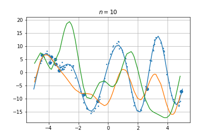
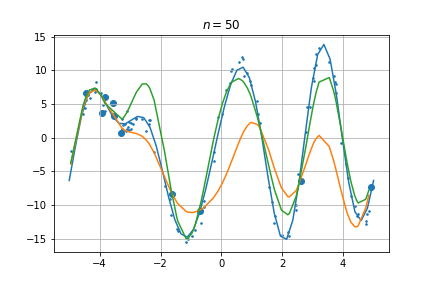
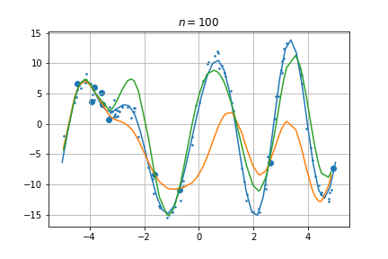
Figure 7: Two sets of examples of predictions on the synthetic, ‘Fourier’ meta-learning problem. Top and bottom rows correspond to different (random) instances; the top row in fact replicates Fig. 1. Training data is shown in bold, small dots show test data. We also show the predictions for two learners (at every input) and the target function. The column correspond to outputs obtained training on $n\in\{10,50,100\}$ tasks.

For completeness, the pseudocode of MoM is given in Algorithm 2.

Algorithm 2 MoM Estimator for Learning Linear Features of (Tripuraneni et al., 2020)

0:  $\left((\bm{x}_{1,j},y_{1,j})\right)_{j=1}^{m_{1}},\ldots,\left((\bm{x}_{m_{n-1},j},y_{m_{n-1},j})\right)_{j=1}^{m_{i-1}}$ — training examples from $n-1$ past tasks, $s$ — problem rank.

  $\bm{U}\bm{D}\bm{V}^{\top}\leftarrow\text{SVD}\left(\frac{1}{M-m_{n}}\sum_{i=1}^{n-1}\sum_{j=1}^{m_{n}}y_{i,j}^{2}\bm{x}_{i,j}\bm{x}_{i,j}^{\top}\right)$

  $\bm{\hat{B}}\leftarrow[D_{1,1}\bm{u}_{1},\ldots,D_{s,s}\bm{u}_{s}]$

  return $\bm{\hat{B}}$

References

- Baxter (1998) Baxter, J. Theoretical models of learning to learn. In S. Thrun, L. P. (ed.), Learning to learn, pp. 71–94. Springer, 1998.
- Baxter (2000) Baxter, J. A model of inductive bias learning. Journal of Artificial Intelligence Research, 12:149–198, 2000.
- Bretagnolle & Huber (1979) Bretagnolle, J. and Huber, C. Estimation des densités: risque minimax. Zeitschrift für Wahrscheinlichkeitstheorie und verwandte Gebiete, 47(2):119–137, 1979.
- Dempster et al. (1977) Dempster, A. P., Laird, N. M., and Rubin, D. B. Maximum likelihood from incomplete data via the em algorithm. Journal of the Royal Statistical Society: Series B (Methodological), 39(1):1–22, 1977.
- Denevi et al. (2018) Denevi, G., Ciliberto, C., Stamos, D., and Pontil, M. Learning to learn around a common mean. In Conference on Neural Information Processing Systems (NeurIPS), pp. 10169–10179, 2018.
- Denevi et al. (2019) Denevi, G., Ciliberto, C., Grazzi, R., and Pontil, M. Learning-to-learn stochastic gradient descent with biased regularization. In International Conference on Machine Learing (ICML), 2019.
- Du et al. (2020) Du, S. S., Hu, W., Kakade, S. M., Lee, J. D., and Lei, Q. Few-shot learning via learning the representation, provably. arXiv:2002.09434, 2020.
- Dua & Graff (2017) Dua, D. and Graff, C. UCI machine learning repository, 2017. URL http://archive.ics.uci.edu/ml.
- Finn et al. (2017) Finn, C., Abbeel, P., and Levine, S. Model-agnostic meta-learning for fast adaptation of deep networks. In International Conference on Machine Learing (ICML), 2017.
- Finn et al. (2019) Finn, C., Rajeswaran, A., Kakade, S., and Levine, S. Online meta-learning. International Conference on Machine Learing (ICML), 2019.
- Khodak et al. (2019a) Khodak, M., Balcan, M.-F., and Talwalkar, A. Provable guarantees for gradient-based meta-learning. In International Conference on Machine Learing (ICML), pp. 424–433, 2019a.
- Khodak et al. (2019b) Khodak, M., Balcan, M.-F. F., and Talwalkar, A. S. Adaptive gradient-based meta-learning methods. Advances in Neural Information Processing Systems, 32:5917–5928, 2019b.
- Kuzborskij & Orabona (2013) Kuzborskij, I. and Orabona, F. Stability and Hypothesis Transfer Learning. In International Conference on Machine Learing (ICML), pp. 942–950, 2013.
- Kuzborskij & Orabona (2016) Kuzborskij, I. and Orabona, F. Fast Rates by Transferring from Auxiliary Hypotheses. Machine Learning, pp. 1–25, 2016. ISSN 1573-0565. doi: 10.1007/s10994-016-5594-4.
- Lattimore & Szepesvári (2018) Lattimore, T. and Szepesvári, C. Bandit algorithms. Cambridge University Press, 2018.
- Lucas et al. (2021) Lucas, J., Ren, M., Kameni, I., Pitassi, T., and Zemel, R. Theoretical bounds on estimation error for meta-learning. In International Conference on Learning Representations, 2021.
- Maurer (2005) Maurer, A. Algorithmic stability and meta-learning. Journal of Machine Learning Research, 6(Jun):967–994, 2005.
- Maurer (2009) Maurer, A. Transfer bounds for linear feature learning. Machine Learning, 75(3):327–350, 2009.
- Maurer et al. (2016) Maurer, A., Pontil, M., and Romera-Paredes, B. The benefit of multitask representation learning. Journal of Machine Learning Research, 2016.
- Pentina & Lampert (2014) Pentina, A. and Lampert, C. A pac-bayesian bound for lifelong learning. In International Conference on Machine Learing (ICML), pp. 991–999, 2014.
- Tripuraneni et al. (2020) Tripuraneni, N., Jin, C., and Jordan, M. I. Provable meta-learning of linear representations. arXiv:2002.11684, 2020.
- Yang et al. (2007) Yang, J., Yan, R., and Hauptmann, A. G. Cross-domain video concept detection using adaptive svms. In Proceedings of the 15th ACM international conference on Multimedia, pp. 188–197, 2007.