Long-term dynamics driven by resonant wave-particle interactions: from Hamiltonian resonance theory to phase space mapping

Abstract

In this study we consider the Hamiltonian approach for the construction of a map for a system with nonlinear resonant interaction, including phase trapping and phase bunching effects. We derive basic equations for a single resonant trajectory analysis and then generalize them into the map in the energy/pitch-angle space. The main advances of this approach are the possibility to consider effects of many resonances and to simulate the evolution of the resonant particle ensemble on long time ranges. For illustrative purposes we consider the system with resonant relativistic electrons and field-aligned whistler-mode waves. The simulation results show that the electron phase space density within the resonant region is flattened with reduction of gradients. This evolution is much faster than the predictions of quasi-linear theory. We discuss further applications of the proposed approach and possible ways for its generalization.

1 Introduction

The resonant wave-particle interaction is known to be one of the main drivers of dynamics of such space plasma systems as planetary radiation belts (e.g., Thorne, 2010; Menietti et al., 2012), collisionless shock waves (e.g., Balikhin et al., 1997; Wilson et al., 2007, 2012; Wang et al., 2020), auroral acceleration region (e.g., Chaston et al., 2008; Watt & Rankin, 2009; Mauk et al., 2017), and solar wind (e.g., Krafft & Volokitin, 2016; Kuzichev et al., 2019; Tong et al., 2019; Yoon et al., 2019; Roberg-Clark et al., 2019). The classical quasi-linear theory (Vedenov et al., 1962; Drummond & Pines, 1962) and its generalizations for inhomogeneous plasma systems (Ryutov, 1969; Lyons & Williams, 1984) describe well charged particle resonant interaction with low-amplitude broadband waves (Karpman, 1974; Shapiro & Sagdeev, 1997; Tao et al., 2012a; Camporeale & Zimbardo, 2015; Allanson et al., 2020).

One of the important examples of application of the quasi-linear theory is the Earth radiation belt models that describe energetic electron acceleration and losses due to resonances with electromagnetic whistler-mode waves and electromagnetic ion cyclotron (EMIC) waves (see reviews Thorne et al., 2010; Shprits et al., 2008; Ni et al., 2016; Nishimura et al., 2010; Millan & Thorne, 2007, and references therein). Moreover, the natural inhomogeneity of the background magnetic field and plasma density in the radiation belts can significantly weaken the conditions of applicability of the quasi-linear theory (Solovev & Shkliar, 1986; Albert, 2001, 2010). However, this theory meets difficulties in describing resonances with sufficiently intense waves (Shapiro & Sagdeev, 1997), when the nonlinear effects of phase trapping and phase bunching become important (Omura et al., 1991; Shklyar & Matsumoto, 2009; Albert et al., 2013; Artemyev et al., 2018a). Indeed, sufficiently intense whistler-mode waves are frequently observed in the radiation belts (Cattell et al., 2008; Wilson et al., 2011; Agapitov et al., 2014) and contribute significantly to wave statistics (Zhang et al., 2018, 2019; Tyler et al., 2019). Theoretically, phase trapping and bunching (also called nonlinear scattering) effects are responsible for fast acceleration (e.g., Demekhov et al., 2006, 2009; Omura et al., 2007; Hsieh & Omura, 2017; Hsieh et al., 2020) and losses (e.g., Kubota et al., 2015; Kubota & Omura, 2017; Grach & Demekhov, 2020) of energetic electrons and for the generation of coherent whistler-mode waves (Demekhov, 2011; Katoh, 2014; Katoh & Omura, 2016; Tao, 2014; Omura et al., 2008, 2013; Nunn & Omura, 2012). There are many observational evidences of such nonlinear resonant wave generation (Titova et al., 2003; Cully et al., 2011; Tao et al., 2012b; Mourenas et al., 2015) and of the related electron acceleration/losses (e.g., Foster et al., 2014; Agapitov et al., 2015b; Mourenas et al., 2016a; Chen et al., 2020).

The quasi-linear diffusion theory describes a sufficiently weak scattering in energy/pitch-angle space and operates with a Fokker-Planck diffusion equation for the charged particle distribution function (Andronov & Trakhtengerts, 1964; Kennel & Engelmann, 1966; Lerche, 1968). In contrast to this description, the nonlinear phase trapping assumes a fast transport in energy/pitch-angle space (e.g., Artemyev et al., 2014a; Furuya et al., 2008), when even a single resonant interaction changes significantly the electron’s energy/pitch-angle (e.g., Albert et al., 2013; Artemyev et al., 2018a). This essentially non-diffusive process cannot be directly included into the Fokker-Planck equation. One possible approach is the construction of an operator that would describe fast charged particle jumps in the energy/pitch-angle; this operator can be constructed with the numerical (test-particle) approach (e.g., Hsieh & Omura, 2017; Zheng et al., 2019) or with the analytical calculation of jumps’ probabilities (e.g., Vainchtein et al., 2018). The main advantage of this approach is the inclusion of almost arbitrary (as realistic as needed) wave spectrum and characteristics (e.g., wave modulation and frequency drifts, see Kubota & Omura, 2018; Artemyev et al., 2019b; Hiraga & Omura, 2020). The main disadvantages are an accumulation of numerical errors with running time, and the almost intractable fine details of the energy/pitch-angle space binning needed to simultaneously resolve large jumps due to trapping and small changes due to drift/diffusion.

An alternative approach to the construction of such an operator is a generalization of the Fokker-Planck equation to include effects of phase trapping and phase bunching (Solovev & Shkliar, 1986; Artemyev et al., 2016b, 2017). This approach is based on a fine balance of trappings and bunchings for a single wave system (e.g., Shklyar, 2011; Artemyev et al., 2019a). The main advantage of this approach is that the evolution of charged particle distribution function can be investigated in arbitrary details in presence of phase trapping, phase bunching, and diffusion (Artemyev et al., 2018b, 2019a, e.g.,). The main disadvantage is that there is no straightforward generalization of this approach for multi-wave (multi-resonance) systems. A single-wave resonance results in charged particle transport in the energy/pitch-angle space along 1D curves, so-called resonance surface curves (e.g., Lyons & Williams, 1984; Summers et al., 1998), and the Fokker-Planck equation with trapping was derived for such a quasi-1D system (Artemyev et al., 2016b).

Another alternative for the description of charged particle distribution evolution driven by nonlinear wave-particle interaction (phase trapping and bunching) is the mapping technique that describes the characteristics of the Fokker-Planck equation (Van Kampen, 2003). The classical example of this approach is the Chirikov map (Chirikov, 1979), which describes particle diffusion and is widely used for systems with wave-particle resonances (e.g., Vasilev et al., 1988; Zaslavskii et al., 1989; Benkadda et al., 1996; Khazanov et al., 2013, 2014). Such a map has been constructed for a single-wave system with phase-trapping and phase bunching effects (Artemyev et al., 2020b). In this study we show the generalization of this map for a multi-resonance system.

We consider a strong magnetic field system, where charged particle motion is well gyrotropic and magnetic moments are well conserved away from the resonances. Thus, 3D velocity space can be reduced to 2D energy/pitch-angle space. The mapping for this space should describe 2D charged particle motion due to energy/pitch-angle jumps with the time-intervals between jumps equal to the interval between passages through the resonances. Diffusive jumps (with zero mean values) and jumps driven by nonlinear phase bunching and phase trapping depend on the resonant phase $\varphi_{R}$, i.e. a variable proportional to the particle gyrophase, which changes fast. In low wave intensity systems this phase is randomly distributed over entire ($\varphi_{R}\in[0,2\pi]$) range, and the phase dependence $\sim\sin\varphi_{R}$ can be directly included into the map (Vasilev et al., 1988; Zaslavskii et al., 1989; Benkadda et al., 1996; Khazanov et al., 2013, 2014). The phase bunching and phase trapping operate in certain $\varphi_{R}$ ranges (e.g., Albert, 1993; Itin et al., 2000; Grach & Demekhov, 2020), whereas jumps depend on $\varphi_{R}$ quite nonmonotonically (see Artemyev et al. (2014b, 2018a)). However, due to phase randomization between two successive resonances (see Appendix in (Artemyev et al., 2020b)), the phase-dependence can be reduced to a simplified determination of ranges corresponding to phase trapping $\varphi_{R}\in[0,2\pi\Pi]$ and phase bunching $\varphi_{R}\in[\Pi,2\pi]$ where $\Pi<1$ is the probability of trapping (see, e.g., Artemyev et al. (2018a)). The phase gain between two resonances is a large value depending on particle energy and pitch-angle, but this dependence can be omitted in the leading approximation (see discussion in Artemyev et al. (2020b)). Therefore, in this study we consider charged particle transport in the energy/pitch-angle space due to nonlinear resonant interaction under assumption of resonant phase randomization (limitations of this assumption have been studied in Artemyev et al. (2020a)).

The paper structure includes a description of the basic system properties and examples of multi-resonant systems observed in the Earth’s radiation belts (Sect. 1). We present three examples: with two whistler-mode waves providing two cyclotron resonances, with one oblique whistler-mode wave providing cyclotron and Landau resonances, and with one whistler-mode wave and one EMIC wave providing two different cyclotron resonances. Then we focus on the first example and construct the map for this system (Sect. 2). Theoretical results derived from this map are verified with test particle simulations. At the end of the paper we discuss the constructed map and possible extensions of the proposed approach (Sect. 3).

2 Basic system properties

The Hamiltonian of a relativistic charged particle (e.g., an electron with rest mass $m_{e}$ and charge $-e$) moving in the 2D inhomogeneous magnetic field of the Earth dipole and interacting with electromagnetic waves (in the low amplitude limit with the wave energy $U_{w}$ much smaller than electron energy $\sim m_{e}c^{2}$, where $c$ is the speed of light) can be written as (e.g., Albert et al., 2013; Artemyev et al., 2018b):

$$H = m_{e}c^{2}\gamma+U_{w}\left({s,I_{x}}\right)\sin\left({\phi\pm n\psi}\right)$$

$$\gamma = \sqrt{1+\frac{{p_{\parallel}^{2}}}{{m_{e}^{2}c^{2}}}+\frac{{2I_{x}\Omega_{ce}}}{{m_{e}c^{2}}}},$$ (1)

where two pairs of conjugate variables are $(s,p_{\parallel})$ (the field-aligned coordinate and momentum) and $(\psi,I_{x})$ (gyrophase and momentum $I_{x}=c\mu/e$; $\mu$ is the classical magnetic moment). The electron gyrofrequency $\Omega_{ce}=eB_{0}/m_{e}c$ is determined by the background magnetic field $B_{0}(s)$, given by, e.g., the reduced dipole model (Bell, 1984). The sign $\pm$ in front of $\psi$ is determined by the wave polarization: $+$ for whistler-mode waves interacting with electrons and $-$ for EMIC waves interacting with electrons. The resonance number is $n=0,\pm 1,\pm 2...$. The wave vector ${\bf k}=(k_{\parallel}(\omega,s),k_{\perp}(\omega,s))$ is given by cold plasma dispersion equation (Stix, 1962) for a constant wave frequency $\omega$ (i.e., $\partial\phi/\partial s=k_{\parallel}$, $\partial\phi/\partial t=\omega$). For a finite angle $\theta={\rm arctan}(k_{\perp}/k_{\parallel})$ between the wave vector and the background magnetic field the wave amplitude in Hamiltonian (1) takes the form (Albert, 1993; Tao & Bortnik, 2010; Nunn & Omura, 2015; Artemyev et al., 2018b):

$$U_{w} = \sqrt{\frac{{2I_{x}\Omega_{ce}}}{{m_{e}c^{2}}}}\frac{{eB_{w}}}{k}\sum\limits_{\pm}{\frac{{\cos\theta\pm C_{1}}}{{2\gamma}}J_{n\pm 1}\left({\sqrt{\frac{{2I_{x}k^{2}}}{{m_{e}\Omega_{ce}}}}\sin\theta}\right)}$$

$$+ \frac{{eB_{w}}}{k}\left({\frac{{p_{\parallel}}}{{\gamma m_{e}c}}+C_{2}}\right)J_{n}\left({\sqrt{\frac{{2I_{x}k^{2}}}{{m_{e}\Omega_{ce}}}}\sin\theta}\right)\sin\theta$$

where $B_{w}$ is the wave magnetic field amplitude, $C_{1,2}$ are functions of wave dispersion and $\theta$, and $J_{n}$ are Bessel functions. Equation (LABEL:eq02) shows that for field-aligned waves $\theta=0$ there is only one cyclotron resonance $n=-1$: $U_{w}=\sqrt{2I_{x}\Omega_{ce}/m_{e}c^{2}}eB_{w}/k\gamma$ (with $C_{1}=1$ for $\theta=0$, see (Tao & Bortnik, 2010)). For oblique wave propagation $\theta\neq 0$ the whole set of resonances with different values of $n$ is present.

2.1 Field-aligned whistler waves

Let us start with the system of two field-aligned whistler waves with the Hamiltonian:

$$H=m_{e}c^{2}\gamma+\sqrt{\frac{{2I_{x}\Omega_{ce}}}{{m_{e}c^{2}}}}\frac{e}{\gamma}\sum\limits_{i=0,1}{\frac{{B_{w,i}}}{{k_{i}}}\sin\left({\phi_{i}+\psi}\right)}$$ (3)

where $\partial\phi_{i}/\partial s=k_{i}=k_{i}(\omega_{i},s)$ with the two different wave frequencies $\omega_{i}$. Figure 1 shows an example of such system observations. THEMIS spacecraft measures waves within the whistler-mode frequency range ($f\in[0.1,1]f_{ce}$; $f_{ce}=\Omega_{ce}/2\pi$): there are two clear maxima in the magnetic and electric field spectra at $f\sim f_{ce}/4$ and $f\sim 3f_{ce}/8$ (see panels (a) and (b)). Both waves propagate along the background magnetic field: panel (c) shows $\theta$ as a function of the frequency. These double-peak spectra are quite typical for whistler-mode waves in the inner magnetosphere (see, e.g., Meredith et al., 2007; Ma et al., 2017; Crabtree et al., 2017; Zhang et al., 2020b; He et al., 2020; Yu et al., 2020).

To study electron energy/pitch-angle variation in the system with Hamiltonian (3), we follow the standard procedure (Neishtadt & Vasiliev, 2006; Neishtadt, 2014) and introduce the wave phases as new canonical variables, $\varphi_{i}=\phi_{i}+\psi$, with the generating function:

$$W=sP+\left({\int{k_{0}(\tilde{s})d\tilde{s}}-\omega_{0}t+\psi}\right)I_{0}+\left({\int{k_{1}(\tilde{s})d\tilde{s}}-\omega_{1}t+\psi}\right)I_{1}$$ (4)

This function gives new variables: $P=p-k_{0}I_{0}-k_{1}I_{1}$, $S=s$ (we keep $s$ notation), $I_{x}=I_{0}+I_{1}$, and new Hamiltonian $H_{I}=H+\partial W/\partial t=H-\omega_{0}I_{0}-\omega_{1}I_{1}$

$$H_{I} = -\omega_{0}I_{0}-\omega_{1}I_{1}+m_{e}c^{2}\gamma+\sqrt{\frac{{2\left({I_{0}+I_{1}}\right)\Omega_{ce}}}{{m_{e}c^{2}}}}\frac{e}{\gamma}\sum\limits_{i=0,1}{\frac{{B_{w,i}}}{{k_{i}}}\sin\varphi_{i}}$$

$$\gamma = \sqrt{1+\frac{{\left({P+k_{0}I_{0}+k_{1}I_{1}}\right)^{2}}}{{m_{e}^{2}c^{2}}}+\frac{{2\left({I_{0}+I_{1}}\right)\Omega_{ce}}}{{m_{e}c^{2}}}}$$

Hamiltonian $H_{I}$ describes a conservative system ($H_{I}={\rm const}$; without loss of generality we take $H_{I}={0}$) with three degrees of freedom, i.e., with three pairs of conjugate variables $(s,P)$, $(\varphi_{0},I_{0})$, $(\varphi_{1},I_{1})$. The resonance $\dot{\varphi}_{i}=0$ conditions give $I_{0}=I_{0R}(s,P,I_{1})$, $I_{1}=I_{1R}(s,P,I_{0})$ as solutions of equations $\omega_{i}=m_{e}c^{2}\partial\gamma/\partial I_{i}=0$. Thus, there are two resonant surfaces. If these surfaces cross (i.e., at the same $s,P$ electron can have simultaneously $I_{0}=I_{0R}$ and $I_{1}=I_{1R}$),then electrons can simultaneously be in resonance with the two waves (Shklyar & Zimbardo, 2014; Zaslavsky et al., 2008). This quite complicated system would require a separate consideration (Sagdeev et al., 1988; Lichtenberg & Lieberman, 1983). Hereafter, we focus instead on the simpler case of well-separated resonances, when resonant surfaces do not cross. Equations $I_{0}=I_{0R}$ and $I_{1}=I_{1R}$ together with the condition $H_{I}={0}$ determine two families of curves in in $(s,P)$ plane; values $I_{0}$ and $I_{1}$ are parameters of these families. Thus, on the curve $I_{0}=I_{0R}(s,P,I_{1})$ there is no change of $I_{1}$, and on the curve $I_{1}=I_{1R}(s,P,I_{0})$ there is no change of $I_{0}$. With constant $I_{1}$ (or $I_{0}$) the $I_{0}$ (or $I_{1}$) variation is directly related to the variation of energy: $-\omega_{0}I_{0}-\omega_{1}I_{1}+m_{e}c^{2}\gamma=0$. Taking into account that $I_{0}+I_{1}=I_{x}=m_{e}c^{2}(\gamma^{2}-1)\sin^{2}\alpha_{eq}/2$, we can plot resonance curves (e.g., Lyons & Williams, 1984; Summers et al., 1998; Mourenas et al., 2012), along which $I_{i}$ change, in the energy/pitch-angle space ($m_{e}c^{2}(\gamma-1),\alpha_{eq}$) (note that we use the equatorial pitch-angle $\alpha_{eq}$ defined at the minimum of $B_{0}(s)$ field, i.e., at the minimum of $\Omega_{ce}(s)$). Figure 1(d) shows these curves $m_{e}c^{2}\gamma-\omega_{i}I_{i}={\rm const}$: each curve of $I_{0}$ change corresponds to a fixed value of $I_{1}$, and vice versa. Electrons move along these curves with the time-step of the interval between resonances. Note between resonances both $I_{i}$ and $\gamma$ are conserved, and electrons are moving along adiabatic orbits without wave influence, i.e. energy and pitch-angle change only at the resonances.

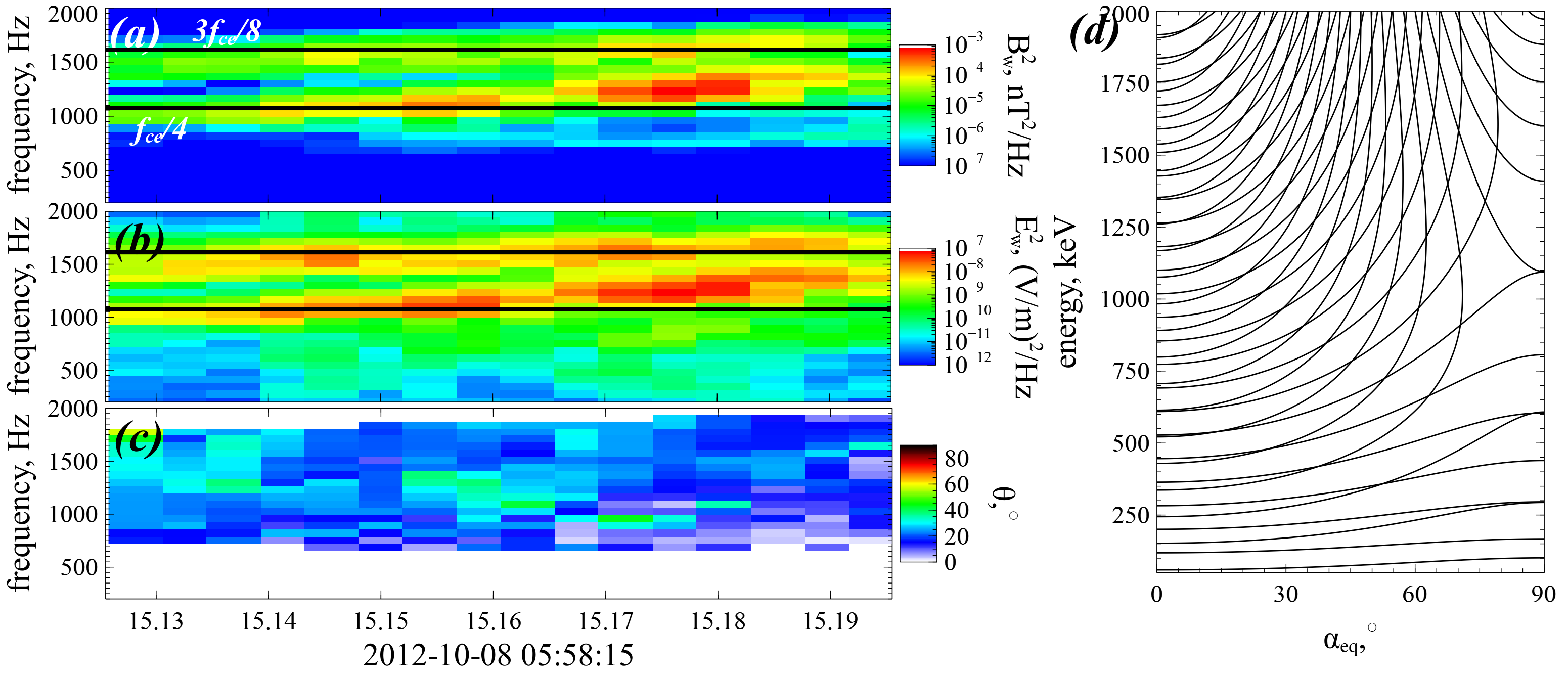
Figure 1: Observational example of two whistler-mode waves by Van Allen Probe A Mauk et al. (2013): magnetic field spectrum (a) and electric field spectrum (b) are obtained from EMFISIS measurements Kletzing et al. (2013), wave-normal angle (c) is estimated using the singular value decomposition method Santolík et al. (2003). Resonance curves for the system with two observed whistler-mode waves (d).

Let us consider electron dynamics in the energy/pitch-angle space for the system with Hamiltonian (3). We numerically integrate Hamiltonian equations for systems with a single wave and with two waves. Figures 2(a,b) show electron motion in the energy/pitch-angle space due to the resonance with a single wave. Solid curves are resonant curves of $-\omega_{0}I_{0}-\omega_{1}I_{1}+m_{e}c^{2}\gamma={\rm const}$ for the wave frequency $\omega_{0}$ and for the wave frequency $\omega_{1}$. Electrons move along this curve due to phase bunching (small negative jumps of energy and pitch-angle; see bottom panels) and phase trapping (rare large positive jumps of energy and pitch-angle; see bottom panels). Conservation of $-\omega_{0}I_{0}-\omega_{1}I_{1}+m_{e}c^{2}\gamma$ and one of the momenta ($I_{0}$ or $I_{1}$) makes electron dynamics 1D in the energy/pitch-angle space. However, this dynamics becomes 2D in the system with two waves, when both $I_{0}$ and $I_{1}$ change, see Fig. 2(c). The electron moves along resonance curves and jumps between these curves due to $I_{i}$ jumps. There are still the same energy and pitch-angle jumps due to phase bunching and phase trapping (see bottom panels), but electron phase trajectory covers the entire energy/pitch-angle space. We describe this 2D dynamics with the mapping technique in this study.

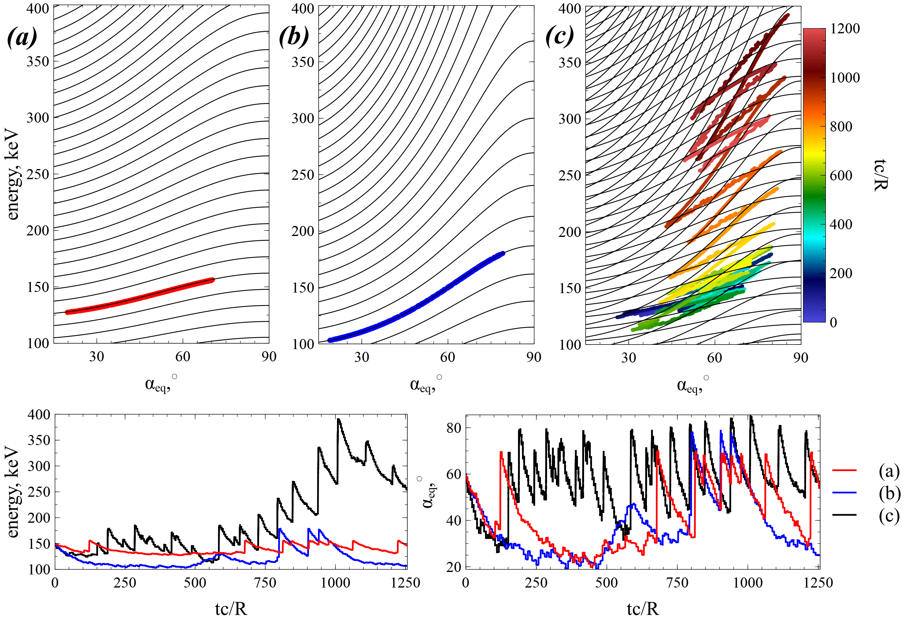
Figure 2: Top panels show resonance curves (black) and electron trajectories in the energy/pitch-angle space for Hamiltonian (3): only the first whistler-mode wave (a), only the second whistler-mode wave (b), both whistler-mode waves (c). In panel (c) different colors correspond to different time intervals. The bottom panels show energy and pitch-angle time series for the three trajectories in the top panels. We use parameters of dipole field at a radial distance of $\sim 5$ Earth radii. Plasma density is given by the model from Sheeley et al. (2001) and constant along magnetic field lines. Wave frequencies are $\omega_{0}=0.4\Omega_{ce}$, $\omega_{1}=0.2\Omega_{ce}$. Both wave amplitudes are $300$ pT (see discussion of such wave observations in Zhang et al., 2018; Tyler et al., 2019). Wave amplitude is distributed along magnetic field line as $\tanh((\lambda/\delta\lambda_{1})^{2})\exp(-(\lambda/\delta\lambda_{2})^{2})$ with $\lambda$ the magnetic latitude ($ds=Rd\lambda\sqrt{1+\sin^{2}\lambda}\cos\lambda$) and $\delta\lambda_{1}=2^{\circ}$, $\delta\lambda_{2}=20^{\circ}$. This function fits the observed whistler-mode wave intensity distribution Agapitov et al. (2013).

2.2 Oblique whistler-mode wave

The second example corresponds to electron resonant interaction with a single oblique ($\theta\neq 0$) wave, for which Hamiltonian (1) takes the form

$$H = m_{e}c^{2}\gamma+\frac{{eB_{w}}}{{k\gamma}}h_{0}\sin\left(\phi\right)+\sqrt{\frac{{2I_{x}\Omega_{ce}}}{{m_{e}c^{2}}}}h_{1}\frac{{eB_{w}}}{{k\gamma}}\sin\left({\phi+\psi}\right)$$

$$h_{0} = -\sqrt{\frac{{2I_{x}\Omega_{ce}}}{{m_{e}c^{2}}}}C_{1}J_{1}+\left({\frac{{p_{\parallel}}}{{m_{e}c}}+C_{2}}\right)J_{0}\sin\theta$$ (6)

$$h_{1} = \frac{1}{2}\left(J_{2}{\left({\cos\theta+C_{1}}\right)+J_{0}\left({\cos\theta-C_{1}}\right)}\right)+\left({\frac{{p_{\parallel}}}{{m_{e}c}}+C_{2}}\right)\frac{{kc}}{{2\Omega_{ce}}}\left({J_{2}+J_{0}}\right)\sin\theta$$

where we restrict our consideration to the first two resonances: Landau resonance $n=0$ and the first cyclotron resonance $n=1$. The Bessel function argument is $\sqrt{2I_{x}k^{2}/m_{e}\Omega_{ce}}\sin\theta$. Such oblique whistler-mode waves are widely observed in the radiation belts (Agapitov et al., 2013, 2015a; Li et al., 2016), and their amplitudes are often sufficiently high for nonlinear resonances (Agapitov et al., 2015b; Artemyev et al., 2016a; Mourenas et al., 2016a). Figure 3 shows an example of oblique whistler-mode wave measured by THEMIS spacecraft in the outer radiation belt. Electric and magnetic field spectra show the one wave power maximum around $f/f_{ce}\sim 1/5$ (see panels (a)&(b)), i.e. this is a single wave. Wave normal angle $\theta\approx 70^{\circ}$ (see panel (c)), i.e., this wave propagates obliquely to the background magnetic field.

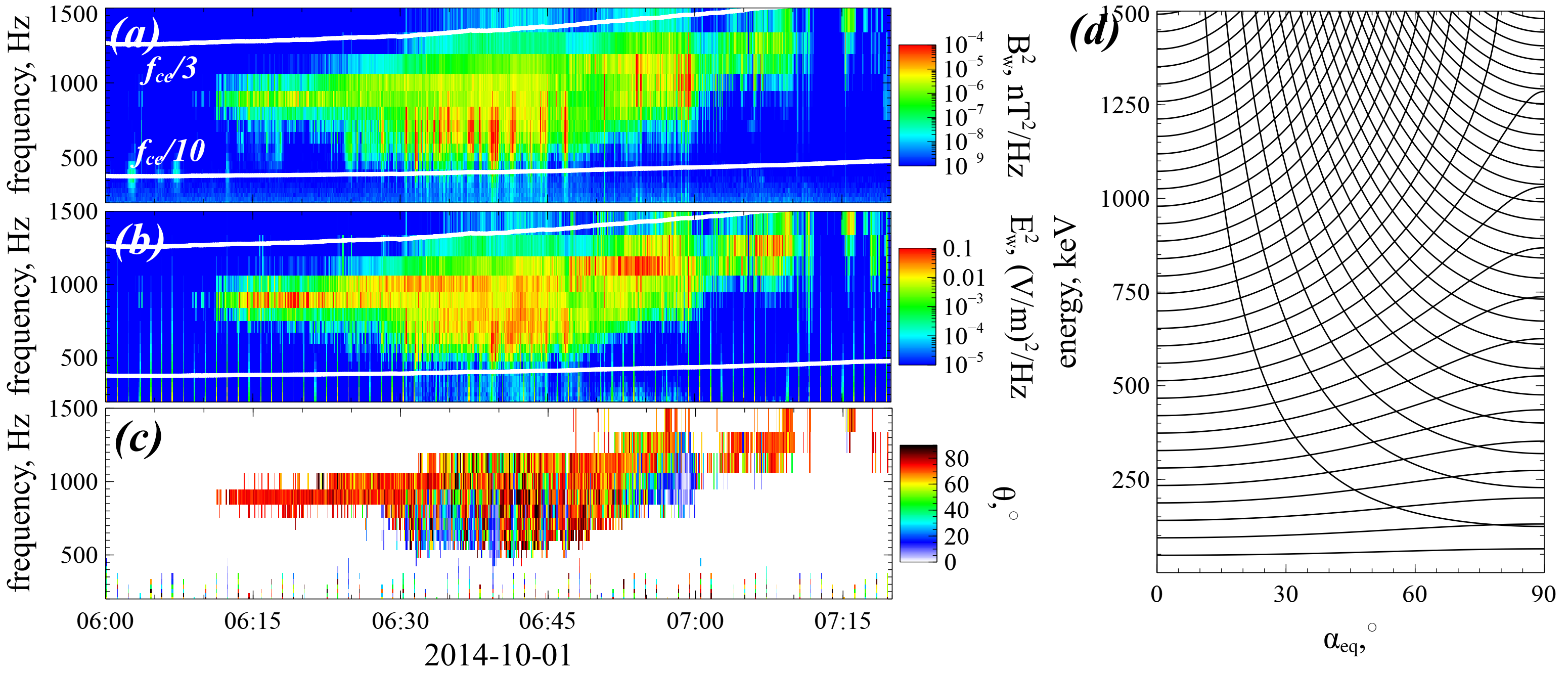
Figure 3: Observational example of oblique whistler-mode wave by Van Allen Probe A Mauk et al. (2013): magnetic field spectrum (a) and electric field spectrum (b) are obtained from EMFISIS measurements Kletzing et al. (2013), wave-normal angle (c) is estimated using using the singular value decomposition method Santolík et al. (2003). Resonance curves for the system with two observed whistler-mode waves (d).

Using the same approach as the one we applied for Hamiltonian (3), we introduce wave phases as new variables, $\varphi_{0}=\phi_{0}$ and $\varphi_{1}=\phi_{1}+\psi$, using the generating function (Neishtadt & Vasiliev, 2006; Neishtadt, 2014):

$$W=sP+\left({\int{k(\tilde{s})d\tilde{s}}-\omega t}\right)I_{0}+\left({\int{k(\tilde{s})d\tilde{s}}-\omega t+\psi}\right)I_{1}$$ (7)

This function gives the new variables: $P=p-k_{0}I_{0}-k_{1}I_{1}$, $S=s$ (we keep $s$ notation), $I_{x}=I_{1}$, and new Hamiltonian $H_{I}=H+\partial W/\partial t=H-\omega I_{0}-\omega I_{1}$

$$H_{I} = -\omega I_{0}-\omega I_{1}+m_{e}c^{2}\gamma+\frac{{eB_{w}h_{0}}}{{k\gamma}}\sin\varphi_{0}+\sqrt{\frac{{2I_{1}\Omega_{ce}}}{{m_{e}c^{2}}}}\frac{{eB_{w}h_{1}}}{{k\gamma}}\sin\varphi_{1}$$ (8)

$$\gamma = \sqrt{1+\frac{{\left({P+k_{0}I_{0}+k_{1}I_{1}}\right)^{2}}}{{m_{e}^{2}c^{2}}}+\frac{{2I_{1}\Omega_{ce}}}{{m_{e}c^{2}}}}$$

The resonance curves in the energy/pitch-angle space are given by two equations: $m_{e}c^{2}\gamma-\omega I_{1}={\rm const}$ with $I_{1}=I_{x}=(\gamma^{2}-1)\sin^{2}\alpha_{eq}/2$ for the cyclotron resonance, and $I_{x}={\rm const}$ for the Landau resonance. Figure 3(d) shows that at $\alpha_{eq}<\pi/4$ Landau resonance curves cross cyclotron resonance curves almost transversely, i.e., in the Landau resonance electrons quickly change energy with weaker pitch-angle change, whereas in the cyclotron resonance the energy change is more effective than the pitch-angle change.

To demonstrate the effects of the two resonances on electron transport in energy/pitch-angle space, we numerically integrate Hamiltonian equations (8) for three systems. Figure 4(a) shows results of the Landau resonance of the electron and oblique whistler-mode wave. The electron moves along a single resonant curve $I_{x}={rmconst}$ with phase bunching responsible for pitch-angle increase and energy decrease, and the phase trapping responsible for pitch-angle decrease and energy increase (bottom panels). Figure 4(b) shows results of the cyclotron resonance: electron motion in the energy/pitch-angle space are quite similar to motions shown in Figs. 2(a&b): phase bunching is responsible for pitch-angle and energy decrease, whereas the phase trapping is responsible for pitch-angle and energy increase (bottom panels). The combination of the two resonances results in rapid electron motion within the whole energy/pitch-angle domain, see Fig. 4(c). The phase bunching decreases electron energy in both resonances, but moves electron in opposite directions in pitch-angle. As a result, a resonant electron loses energy until it reaches the region with high probability of trapping into the Landau resonance (Artemyev et al., 2013). After being trapped in Landau resonance, the electron gains energy and reaches the energy/pitch-angle domain where it can now be trapped into the cyclotron resonance with further energy increase. Such cycles of bunching, Landau trapping, and cyclotron trapping, quickly cover a large energy/pitch-angle domain for a single electron trajectory.

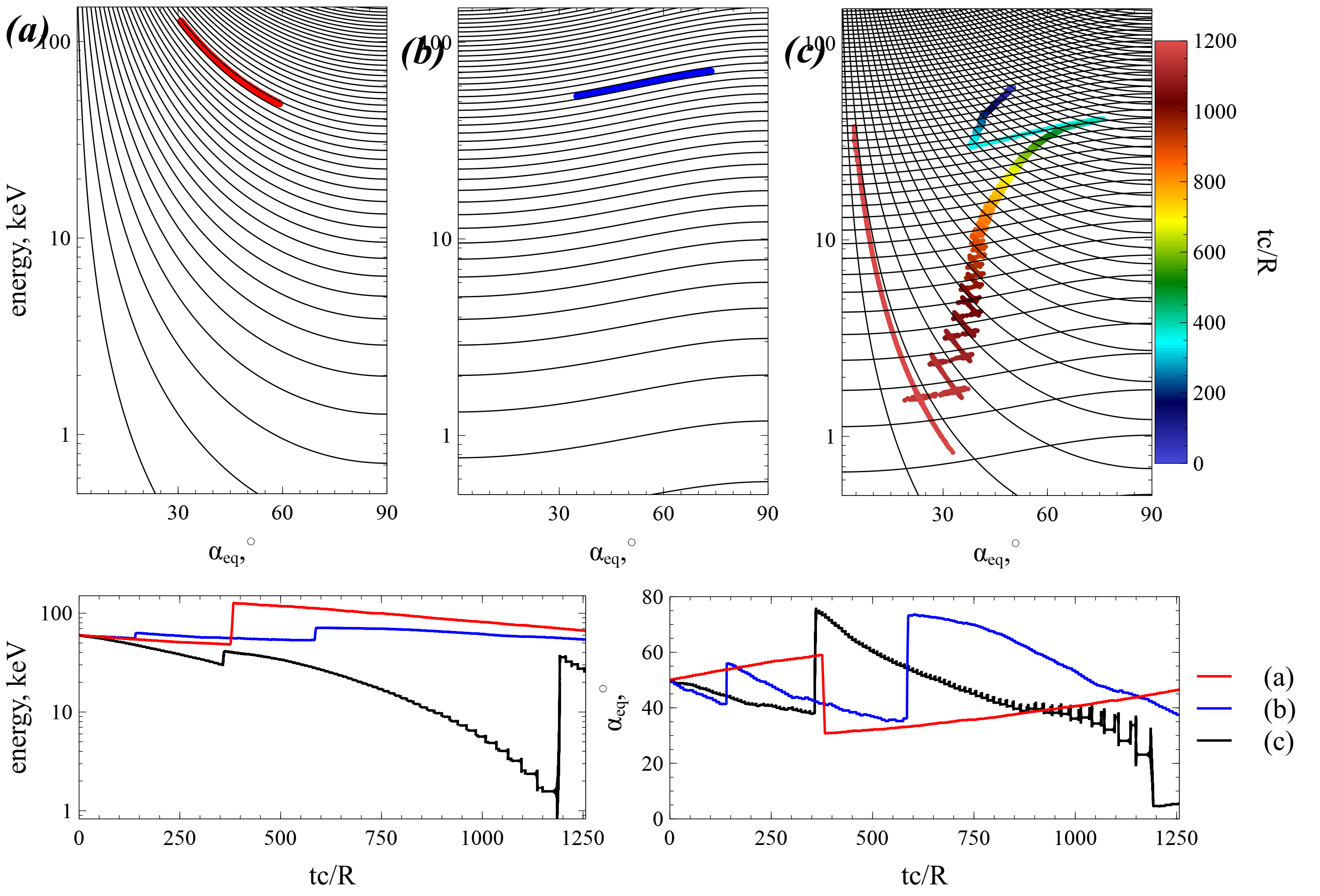
Figure 4: Top panels show resonance curves (black) and electron trajectories in the energy/pitch-angle space for Hamiltonian (6): only Landau resonance (a), only cyclotron resonance (b), both resonances (c). In panel (c) color shows time. Bottom panels show energy and pitch-angle time series for three trajectories from top panels. System parameters are the same as in Fig. 2, wave frequency is $\omega=0.35\Omega_{ce}$, wave amplitude is $500$ pT, and wave normal angle $\theta$ is $5^{\circ}$ away of the resonance cone angle ${\rm acos}(\omega/\Omega_{ce})$ (see discussion of such wave observations in Wilson et al., 2011; Agapitov et al., 2014; Artemyev et al., 2016a; Mourenas et al., 2016a). The wave amplitude distribution along magnetic field-lines is the same as one used in Fig. 1.

2.3 Field-aligned whistler-mode and EMIC waves

A third example is a system with field-aligned whistler-mode wave and field-aligned EMIC wave with polarization opposite to the whistler-mode wave. The corresponding Hamiltonian of a relativistic electron (reduction of Hamiltonian (LABEL:eq02)) takes the form

$$H=m_{e}c^{2}\gamma+\sqrt{\frac{{2I_{x}\Omega_{ce}}}{{m_{e}c^{2}}}}\left({\frac{{eB_{w,0}}}{{k_{0}\gamma}}\sin\left({\phi_{0}+\psi}\right)+\frac{{eB_{w,1}}}{{k_{1}\gamma}}\sin\left({\phi_{1}-\psi}\right)}\right)$$ (9)

where $k_{0}=k_{0}(\omega_{0},s)$ follows the whistler-mode wave dispersion, whereas $k_{1}=k_{1}(\omega_{1},s)$ follows the EMIC wave dispersion. Figure 5(a&b) shows a typical example of observation of such two waves: the high-frequency magnetic field spectrum shows the whistler-mode wave with $f/f_{ce}\sim f_{ce}/2$, whereas the low-frequency magnetic field spectrum shows the EMIC wave with $f/f_{cp}\sim f_{cp}/2$ ($f_{cp}$ is the proton gyrofrequency). The EMIC wave is field-aligned (see panel (c)). Due to the low EMIC wave frequency, the resonance condition $\dot{\phi}_{1}-\dot{\psi}=k_{1}p/\gamma-\omega_{1}-\Omega_{ce}/\gamma=0$ can be reduced to $k_{1}p=\Omega_{ce}$, with typical $k_{1}$ about the inverse ion inertial length (Silin et al., 2011). Thus, only high-energy electrons (with large enough $p$) can resonate with EMIC waves (e.g., in the Earth radiation belts the resonant energy is typically larger than $\sim 1$ MeV, see Thorne & Kennel (1971); Summers & Thorne (2003); Shprits et al. (2016); Chen et al. (2019)). Let us compare whistler-mode and EMIC wave resonance curves for such high energies.

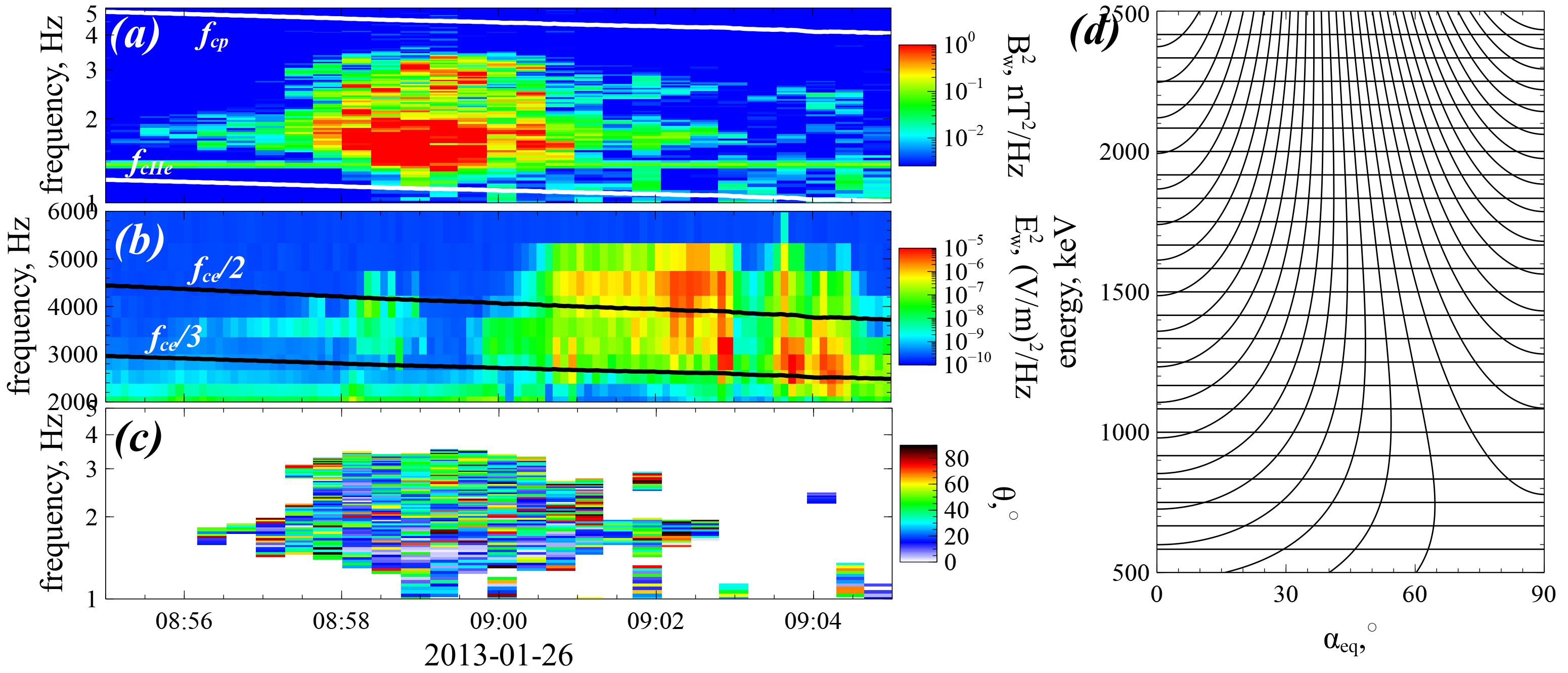
Figure 5: Observational example of a system with whistler-mode and EMIC waves by Van Allen Probe A Mauk et al. (2013): magnetic field spectrum of EMIC wave (a) and whistler-mode wave (b) are obtained from EMFISIS measurements Kletzing et al. (2013), the wave-normal angle of the EMIC wave (c) is estimated using the singular value decomposition method Santolík et al. (2003). Resonance curves for the system with the two observed whistler-mode waves (d).

First, we introduce wave phases as new variables, $\varphi_{0}=\phi_{0}+\psi$ and $\varphi_{1}=\phi_{1}-\psi$, with the generating function (Neishtadt & Vasiliev, 2006; Neishtadt, 2014):

$$W=sP+\left({\int{k_{0}(\tilde{s})d\tilde{s}}-\omega_{0}t+\psi}\right)I_{0}+\left({\int{k_{1}(\tilde{s})d\tilde{s}}-\omega_{1}t-\psi}\right)I_{1}$$ (10)

This function gives new variables: $P=p-k_{0}I_{0}-k_{1}I_{1}$, $S=s$ (we keep $s$ notation), $I_{x}=I_{0}-I_{1}$, and new Hamiltonian $H_{I}=H+\partial W/\partial t=H-\omega I_{0}-\omega I_{1}$

$$H_{I} = -\omega_{1}I_{0}-\omega_{1}I_{1}+m_{e}c^{2}\gamma+\sqrt{\frac{{2\left({I_{0}-I_{1}}\right)\Omega_{ce}}}{{m_{e}c^{2}}}}\sum\limits_{i=0,1}{\frac{{eB_{w,i}}}{{k_{i}\gamma}}\sin\varphi_{i}}$$

$$\gamma = \sqrt{1+\frac{{\left({P+k_{0}I_{0}+k_{1}I_{1}}\right)^{2}}}{{m_{e}^{2}c^{2}}}+\frac{{2\left({I_{0}-I_{1}}\right)\Omega_{ce}}}{{m_{e}c^{2}}}}$$ (11)

The EMIC resonance curves are given by equation $m_{e}c^{2}\gamma-\omega_{1}I_{1}={\rm const}$, and taking into account the smallness of $\omega_{1}$ we obtain $\gamma\approx 0$, i.e. resonance curves are almost straight lines parallel to the energy axis (see Fig. 5(d)). The whistler-mode resonance curves ($m_{e}c^{2}\gamma-\omega_{0}I_{0}={\rm const}$ with $I_{0}=I_{x}+{\rm const}$) cross these lines: the EMIC wave is responsible for electron transport along pitch-angle space, and the whistler-mode wave leads to both pitch-angle and energy changes. Figure 6(a&b) confirms this scenario: the EMIC wave resonates with small pitch-angle (large $p$) electron and phase bunch it to larger pitch-angles (phase trapping by EMIC waves is responsible for pitch-angle decrease; see bottom panel) with an approximate conservation of energy, whereas the whistler-mode wave can resonate with large pitch-angle electrons and transport them to smaller pitch-angles via phase bunching with energy decrease (moving them away from the EMIC wave resonance).

The combination of EMIC and whistler-mode wave resonances (see Fig. 6(c)) can result in a very effective transport of large pitch-angle electrons to small pitch-angles (rapid electron losses): bunching of $\sim 2$ MeV electrons with initially large pitch-angles results in electron transfer to small pitch-angles, where even faster EMIC phase trapping may move this electron to the loss-cone (see discussions of similar effects of combined EMIC and whistler-mode waves in the diffusive approximation in (Mourenas et al., 2016b; Zhang et al., 2017)). From small pitch-angles (note that the loss-cone is not included in our simulations) the EMIC wave can transport an electron via phase bunching to higher pitch-angles, where whistler-mode resonance can accelerate it via trapping. As a result of so different resonant interactions with EMIC and whistler-mode waves, the electron trajectory can quickly fill up a large domain in the energy/pitch-angle space.

Figure 6: Top panels show resonance curves (black) and electron trajectories in the energy/pitch-angle space for Hamiltonian (9): only whistler-mode wave (a), only EMIC wave (b), both whistler-mode and EMIC waves (c). In panel (c) color shows time. Bottom panels show energy and pitch-angle time series for three trajectories in the top panels. System parameters are the same as in Fig. 2. EMIC wave is $H^{+}$ band with the frequency $\omega=0.7\Omega_{cp}$ and amplitude $1$ nT (see discussion of such wave observations in Zhang et al., 2016; Kersten et al., 2014). Whistler-mode wave frequency is $\omega=0.35\Omega_{ce}$, and wave amplitude is $300$ pT. The wave amplitude distribution along magnetic field-lines is the same as one used in Fig. 1.

3 Mapping technique for multi-resonances

To describe the long-term evolution of electron dynamics in the energy/pitch-angle space, we propose to develop a map providing relations for each resonant interaction $\Delta\gamma=\Delta\gamma(\gamma,\alpha_{eq})$, $\Delta\alpha_{eq}=\Delta\alpha(\gamma,\alpha_{eq})$. Changes $\Delta\gamma,\Delta\alpha_{eq}$ are due to phase bunching (nonlinear scattering) and phase trapping. Thus, the first step in the construction of such a map is to derive equations for $\Delta\gamma,\Delta\alpha_{eq}$ driven by both these processes. We start with Hamiltonian (LABEL:eq05) and follow the standard procedure of Hamiltonian expansion around the resonant $I_{0},I_{1}$ values (Neishtadt, 2014; Artemyev et al., 2018a), which are defined by equations $\partial H_{I}/\partial I_{i}=0$:

$$\frac{{k_{i}I_{iR}}}{{m_{e}c}}=-\frac{{P+k_{i^{\prime}}I_{i^{\prime}}}}{{m_{e}c}}-\frac{{\Omega_{ce}}}{{k_{i}}}+\frac{1}{{\sqrt{\left({k_{i}c/\omega_{i}}\right)^{2}-1}}}\sqrt{1-\left({\frac{{\Omega_{ce}}}{{k_{i}c}}}\right)^{2}-2\frac{{\Omega_{ce}}}{{k_{i}c}}\frac{{P+\left({k_{i^{\prime}}-k_{i}}\right)I_{i^{\prime}}}}{{m_{e}c}}}$$ (12)

where $i’=0$ for $i=1$ and $i’=1$ for $i=0$. Expansion of Hamiltonian (LABEL:eq05) around $I_{i}=I_{iR}$ gives

$$H_{Ii} \approx \Lambda_{i}+m_{e}c^{2}\frac{1}{2}g_{i}\left({I_{i}-I_{iR}}\right)^{2}+u_{iR}\sin\varphi_{i}$$

$$\Lambda_{i} = m_{e}c^{2}\gamma_{iR}-\left({\omega_{0}I_{0}+\omega_{1}I_{1}}\right)_{I_{i}=I_{iR}}$$ (13)

$$\gamma_{iR} = \frac{{\left({k_{i}c/\omega_{i}}\right)}}{{\sqrt{\left({k_{i}c/\omega_{i}}\right)^{2}-1}}}\sqrt{1-\left({\frac{{\Omega_{ce}}}{{k_{i}c}}}\right)^{2}-2\frac{{\Omega_{ce}}}{{k_{i}c}}\frac{{P+\left({k_{i^{\prime}}-k_{i}}\right)I_{i^{\prime}}}}{{m_{e}c}}}$$

$$u_{iR} = \sqrt{\frac{{2\Omega_{ce}\left({I_{0}+I_{1}}\right)_{I_{i}=I_{iR}}}}{{m_{e}c^{2}}}}\frac{e}{{\gamma_{iR}}}\frac{{B_{w,i}}}{{k_{i}}}$$

$$g_{i} = \left.{\frac{{\partial^{2}\gamma}}{{\partial I_{i}^{2}}}}\right|_{I_{i}=I_{iR}}=\frac{{k_{i}^{2}}}{{m_{e}^{2}c^{2}}}$$

where $\varphi_{i}$ are fast variables and $I_{i}-I_{iR})$ and $(s,P)$ are slow variables (note that $\Lambda_{i}$ does not depend on fast variables). Next, we introduce new variables $P_{\varphi i}=I_{i}-I_{iR}$ with the generating function $Q_{i}=(I_{i}-I_{iR})\varphi_{i}+s\tilde{P}_{i}$. New Hamiltonians are

$$F_{i} = \Lambda_{i}\left({\tilde{s},\tilde{P}}\right)+m_{e}c^{2}\frac{1}{2}g_{i}P_{\varphi i}^{2}+u_{iR}\sin\varphi_{i}$$

$$\approx \Lambda_{i}\left({s,P}\right)+\left\{{\Lambda_{i},I_{iR}}\right\}_{s,P}\varphi_{i}+m_{e}c^{2}\frac{1}{2}g_{i}P_{\varphi i}^{2}+u_{iR}\sin\varphi_{i}$$

where $\tilde{s}=s-(\partial I_{iR}/\partial P)\varphi_{i}$, $\tilde{P}=p+(\partial I_{iR}/\partial s)\varphi_{i}$, $\{…\}$ are Poisson brackets, and we expand $\Lambda(\tilde{s},\tilde{P})$ over small $\partial I_{iR}/\partial s$, $\partial I_{iR}/\partial P$ terms. Hamiltonian $F_{i}$ is the sum of $\Lambda_{i}(s,P)$ describing slow variable dynamics and pendulum Hamiltonian describing fast variable dynamics:

$$F_{\varphi i}=m_{e}c^{2}\frac{1}{2}g_{i}P_{\varphi i}^{2}+\left\{{\Lambda_{i},I_{iR}}\right\}_{s,P}\varphi_{i}+u_{iR}\sin\varphi_{i}$$ (15)

where the coefficients depend on the slow variables. Figure 7 shows phase portraits of $F_{\varphi i}$ for systems with $a_{i}=|u_{iR}/\{\Lambda_{i},I_{iR}\}|<1$ (panel a) and with $a_{i}=|u_{iR}/\{\Lambda_{i},I_{iR}\}|>1$ (panel b). For low wave amplitude $a_{i}<1$ the phase portrait does not contain closed orbits, i.e., all particles cross the resonance $\dot{\varphi}_{i}=m_{e}c^{2}g_{i}P_{\varphi,i}=0$ within an interval of about one period of $\varphi_{i}$. There are only weak scatterings in this regime with zero mean changes of $I_{i}$, and such scatterings can be described by the quasi-linear diffusion model for inhomogeneous plasma (e.g., Karpman, 1974; Albert, 2010; Grach & Demekhov, 2020). For sufficiently high wave amplitude $a_{i}>1$, however, the phase portrait contains both closed and open orbits, i.e., there are now phase trapped particles oscillating around the resonance $\dot{\varphi}_{i}=m_{e}c^{2}g_{i}P_{\varphi,i}=0$ for a long time. Scattering (crossing of the resonance along the open orbits) would result in phase bunching with a small, yet nonzero mean change of $I_{i}$ (see reviews by Shklyar & Matsumoto, 2009; Albert et al., 2013, and references therein), whereas phase trapping would significantly change $I_{i}$. We would like to include this nonlinear regime of wave-particle interaction into the map in energy/pitch-angle space. For this reason, we derive expressions for changes of $I_{i}$ due to phase bunching, $\Delta_{scat}I_{i}$, and due to phase trapping $\Delta_{trap}I_{i}$. As $\Delta_{scat}I_{i}$ is local, i.e. depends on particle and system characteristics at the resonance, we can keep slow variables unchanged for $\Delta_{scat}I_{i}$ evaluations:

$$\Delta_{scat}I_{i} = 2\int\limits_{-\infty}^{t_{iR}}{\frac{{\partial H_{Ii}}}{{\partial I}}dt}=\frac{{2u_{iR}}}{{m_{e}c^{2}g_{i}}}\int\limits_{-\infty}^{\varphi_{iR}}{\frac{{\cos\varphi_{i}d\varphi_{i}}}{{P_{\varphi i}}}}$$

$$= \sqrt{\frac{{2u_{iR}}}{{m_{e}c^{2}g_{i}}}}\int\limits_{-\infty}^{\varphi_{iR}}{\frac{{\sqrt{u_{iR}}\cos\varphi_{i}d\varphi_{i}}}{{\sqrt{F_{\varphi i}-\left\{{\Lambda_{i},I_{iR}}\right\}_{s,P}\varphi_{i}-u_{iR}\sin\varphi_{i}}}}}$$

$$= \sqrt{\frac{{2u_{iR}}}{{m_{e}c^{2}g_{i}}}}\int\limits_{-\infty}^{\varphi_{iR}}{\frac{{\sqrt{u_{iR}}\cos\varphi_{i}d\varphi_{i}}}{{\sqrt{\left\{{\Lambda_{i},I_{iR}}\right\}_{s,P}\left({\varphi_{Ri}-\varphi_{i}}\right)+u_{iR}\left({\sin\varphi_{Ri}-\sin\varphi_{i}}\right)}}}}$$

$$= \sqrt{\frac{{2u_{iR}}}{{m_{e}c^{2}g_{i}}}}\int\limits_{-\infty}^{\varphi_{iR}}{\frac{{\sqrt{a_{i}}\cos\varphi_{i}d\varphi_{i}}}{{\sqrt{\left({\varphi_{Ri}-\varphi_{i}}\right)+a_{i}\left({\sin\varphi_{Ri}-\sin\varphi_{i}}\right)}}}}=\sqrt{\frac{{2u_{iR}}}{{m_{e}c^{2}g_{i}}}}f_{i}\left({\varphi_{Ri},a_{i}}\right)$$

where $t_{iR}$ is the time of passage through the resonance, $\varphi_{iR}$ is the wave phase at this time, and we use $\dot{\varphi}_{i}=m_{e}c^{2}g_{i}P_{\varphi i}=2^{1/2}\sqrt{F_{\varphi i}-\{\Lambda_{i},I_{iR}\}\varphi_{i}-u_{Ri}\sin\varphi_{i}}$, $F_{\varphi i}=\{\Lambda_{i},I_{iR}\}\varphi_{Ri}+u_{Ri}\sin\varphi_{Ri}$ (resonant energy $F_{\varphi i}$ value evaluated at $P_{\varphi i}=0$). Note Eq. (3) describes $\Delta_{scat}I_{i}$ change for the particle motion thought the resonance from $-\infty$ to resonant $\varphi_{iR}$, whereas the motion in opposite direction would result in change of sign of $\Delta_{scat}I_{i}$. Function $f_{i}(a_{i},\varphi_{iR})$ is periodic for $\varphi_{iR}$, see Fig. 7(c). Although the sign of $f_{i}$ changes within one $\varphi_{iR}$ period, the mean value of this function for $a_{i}>1$ is not zero, providing the effect of phase bunching. To consider the precise $\Delta_{scat}I_{i}$ dependence on $\varphi_{iR}$ in the mapping, one would need to keep information about resonant phase $\varphi_{i}$ and calculate the phase gain between resonances. However, the phase is fast rotating, and even a small change of $\varphi_{i}$ at the resonance would result in a significant change of phase gain between resonances. Therefore, we can assume that $\varphi_{iR}$ is a random variable with a uniform distribution of the resonant energy $F_{\varphi i}(\varphi_{iR})$ at $P_{\varphi i}=0$ axis (see justification of this assumption in Itin et al. (2000); Artemyev et al. (2020a, b)), and all resonant particles with the same slow variables (same energy and pitch-angle) at the resonance would experience the same $\Delta I_{i}$ change equal to $\langle\Delta I_{i}\rangle$ averaged over the resonant energy (Artemyev et al., 2020b).

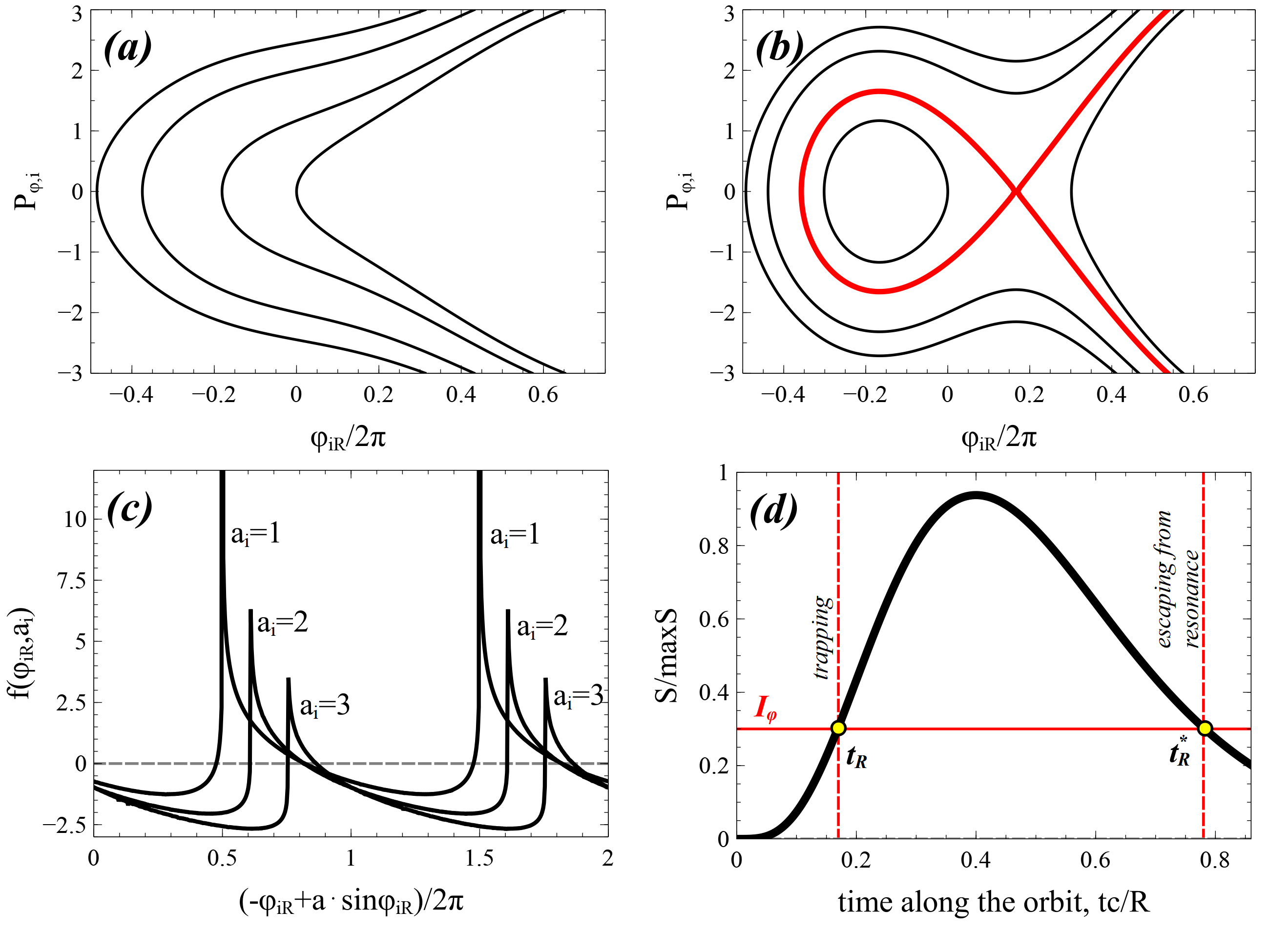
Figure 7: Phase portraits of $F_{\varphi i}$ for systems with $|u_{iR}|<|\{\Lambda_{i},I_{iR}\}|$ (a) and with $|u_{iR}|>|\{\Lambda_{i},I_{iR}\}|$ (b). Black curves show contours of $F_{\varphi,i}={\rm const}$, red curve is the separatrix demarcating region of trapped (closed) electrons orbits and region of transient (open) orbits. Function $f(h_{\phi},a)$ for several $a$ and $(-\varphi_{iR}+a\sin\varphi_{iR})/2\pi$ (c) and scheme of trapping/detrapping (d).

An important property of $f$ function from Eq. (3) is that being averaged over energies in resonance, $F_{\varphi i}=\{\Lambda_{i},I_{iR}\}\varphi_{Ri}+u_{Ri}\sin\varphi_{Ri}$, this function gives

$$\left\langle{f_{i}}\right\rangle=-\sqrt{\frac{m_{e}c^{2}g_{i}}{2u_{iR}}}\frac{S}{{2\pi}}=-\sqrt{\frac{8|u_{iR}|}{a_{i}m_{e}c^{2}g_{i}}}\int\limits_{\varphi_{i-}}^{\varphi_{iR}}{\sqrt{\left({\varphi_{Ri}-\varphi_{i}}\right)+a_{i}\left({\sin\varphi_{Ri}-\sin\varphi_{i}}\right)}d\varphi_{i}}$$ (17)

where $S$ is the area surrounded by the separatrix in the phase portrait in Fig. 7(b) (see details of Eq. (17) derivations in Neishtadt (1999) and Artemyev et al. (2018a)). Therefore, the $\Delta_{scat}I_{i}$ change due to phase bunching is equal to $-S/2\pi$ and for $a_{i}\gg 1$ (i.e. for very weak magnetic field inhomogeneity; note $\{\Lambda_{i},I_{iR}\}\sim\partial/\partial s$) we have $\Delta_{scat}I_{i}=-8\sqrt{2u_{iR}/m_{e}c^{2}g_{i}}$ where $S=16\sqrt{2u_{iR}/m_{e}c^{2}g_{i}}$ is the width of the resonance for large amplitude waves (Palmadesso, 1972; Karimabadi et al., 1990).

The change of $I_{i}$ due to phase bunching (nonlinear scattering) is sufficiently small to consider this process locally in energy/pitch-angle space, i.e., $\Delta_{scat}I_{i}\ll I_{i}$ (see discussion of exceptions for $\Delta_{scat}I_{i}\sim I_{i}$ in Appendix A), whereas the change of $I_{i}$ due to phase trapping is essentially non-local. To evaluate $\Delta_{trap}I_{i}$, we take into account that $I_{i}=I_{iR}$ in the resonance (during the trapping), the trapping time is defined as $2\pi I_{\phi}=\int{P_{\varphi i}d\varphi_{iR}}=S$, and $I_{\phi}$ is conserved during the trapping (because trapped particles oscillate in the $(\varphi_{iR},P_{\phi i})$ plane much faster than the system evolves (much faster than variations of slow variables $s,P$). Thus, the trapping time is defined as the time of arrival to the resonance $t_{R}$ with $\dot{S}(t_{R})>0$ (the growth of the area surrounded by the separatrix allows trapping of particles moving along open trajectories into closed trajectories), whereas the time $t_{R}^{*}$ of escape from the trapping is defined by $S(t_{R}^{*})=S(t_{R})$ and $\dot{S}(t_{R}^{*})<0$ (see scheme in Fig. 7(d)):

$$\Delta_{trap}I_{i}=I_{iR}\left({t_{iR}^{*}}\right)-I_{iR}\left({t_{iR}}\right),\quad S\left({t_{iR}^{*}}\right)=S\left({t_{iR}}\right),\quad\dot{S}\left({t_{iR}}\right)>0,\quad\dot{S}\left({t_{iR}^{*}}\right)<0$$ (18)

At the resonance, an electron can be scattered (i.e., experience the phase bunching) or trapped, and this depends on the $\varphi_{iR}$ value (e.g., Albert, 1993; Itin et al., 2000; Grach & Demekhov, 2018). However, as $\varphi_{iR}$ is a fast oscillating variable, we can consider the so-called probability of trapping instead of tracing the precise $\varphi_{iR}$ value: the range of $\varphi_{iR}$ of trapped particles, i.e., the ratio of trapped particles to the total number of resonant particles for a single resonance, is the probability of trapping, $\Pi_{i}$ (e.g., Arnold et al., 2006, and references therein). For small $\Pi_{i}$, this probability is defined as the ratio of the change of the area under the separatrix, $\dot{S}$, and the total resonant flux $\int_{0}^{2\pi}\dot{P}_{\varphi,i}d\phi=2\pi\{\Lambda_{i},I_{iR}\}$: $\Pi_{i}=\dot{S}/2\pi\{\Lambda_{i},I_{iR}\}=\{S,F_{i}\}/2\pi\{\Lambda_{i},I_{iR}\}$. This definition of the trapping probability has been verified for various plasma systems (e.g., Artemyev et al., 2014b; Leoncini et al., 2018; Vainchtein et al., 2018). Therefore, the resonant interaction can be characterized by $\Pi$, $\Delta_{trap}I_{i}$, and $\Delta_{scat}I_{i}$.

Due to conservation of $H_{i}=m_{e}c^{2}\gamma-\omega_{0}I_{0}-\omega_{1}I_{1}$, changes of $I_{i}$ are directly related to $\gamma$ changes, whereas the $I_{x}=I_{0}+I_{1}$ relation gives the pitch-angle change:

$$\frac{{\omega_{i}\sin^{2}\alpha_{eq}}}{{\gamma^{2}-1}}\left({\Delta_{i}\gamma}\right)^{2}-2\Delta_{i}\gamma\frac{{\Omega_{eq}-\gamma\omega_{i}\sin^{2}\alpha_{eq}}}{{\gamma^{2}-1}}$$

$$+ \omega_{i}\left({\sin^{2}\left({\alpha_{eq}+\Delta_{i}\alpha_{eq}}\right)-\sin^{2}\alpha_{eq}}\right)=0$$

that for small changes (phase bunching) can be rewritten as

$$\Delta_{i}\alpha_{eq}=\Delta_{i}\gamma\frac{{\Omega_{eq}-\gamma\omega_{i}\sin^{2}\alpha_{eq}}}{{\omega_{i}\sin\alpha_{eq}\cos\alpha_{eq}\left({\gamma^{2}-1}\right)}}$$ (19)

Therefore, the map for one resonance can be written as

$$\begin{array}[]{l}\left({\begin{array}[]{*{20}c}{\bar{\gamma}}\\ {\bar{\alpha}_{eq}}\\ \end{array}}\right)=\left({\begin{array}[]{*{20}c}{G_{\gamma i}\left({\gamma,\alpha_{eq}}\right)}\\ {G_{\alpha i}\left({\gamma,\alpha_{eq}}\right)}\\ \end{array}}\right)=\left({\begin{array}[]{*{20}c}\gamma\\ {\alpha_{eq}}\\ \end{array}}\right)+\left({\begin{array}[]{*{20}c}{\Delta_{i}\gamma}\\ {\Delta_{i}\alpha_{eq}}\\ \end{array}}\right)\\ \Delta_{i}\gamma=\omega_{i}\left\{{\begin{array}[]{*{20}c}{\Delta_{scat}I_{i}\left({\gamma,\alpha_{eq}}\right),}&{\xi_{i}\in\left[{\Pi_{i}\left({\gamma,\alpha_{eq}}\right),1}\right]}\\ {\Delta_{trap}I_{i}\left({\gamma,\alpha_{eq}}\right),}&{\xi_{i}\in\left[{0,\Pi_{i}\left({\gamma,\alpha_{eq}}\right)}\right)}\\ \end{array}}\right.\\ \Delta_{i}\alpha_{eq}=\left\{{\begin{array}[]{*{20}c}{\frac{{\Omega_{eq}-\gamma\omega_{i}\sin^{2}\alpha_{eq}}}{{\sin\alpha_{eq}\cos\alpha_{eq}\left({\gamma^{2}-1}\right)}}\Delta_{scat}I_{i}\left({\gamma,\alpha_{eq}}\right),}&{\xi_{i}\in\left[{\Pi_{i}\left({\gamma,\alpha_{eq}}\right),1}\right]}\\ {\Delta_{i}\alpha_{eq}\left({\Delta_{trap}I_{i},\gamma,\alpha_{eq}}\right),}&{\xi_{i}\in\left[{0,\Pi_{i}\left({\gamma,\alpha_{eq}}\right)}\right)}\\ \end{array}}\right.\\ \end{array}$$ (20)

where $\xi_{i}$ is a random variable uniformly distributed in $[0,1]$. If there are two resonances (one with the first wave and another one with the second wave) during one electron bounce period $\tau_{b}$, then over this period the electron energy/pitch-angle change should be

$$\left({\begin{array}[]{*{20}c}{\bar{\gamma}}\\ {\bar{\alpha}_{eq}}\\ \end{array}}\right)=\left({\begin{array}[]{*{20}c}{G_{\gamma 1}\left({G_{\gamma 0}\left({\gamma,\alpha_{eq}}\right),G_{\alpha 0}\left({\gamma,\alpha_{eq}}\right)}\right)}\\ {G_{\alpha 1}\left({G_{\gamma 0}\left({\gamma,\alpha_{eq}}\right),G_{\alpha 0}\left({\gamma,\alpha_{eq}}\right)}\right)}\\ \end{array}}\right)\quad$$ (21)

Figure 8 shows ten main characteristics of map (21) in the energy/pitch-angle space: amplitudes of scattering $\Delta_{scat,i}\gamma$, $\Delta_{scat,i}\alpha_{eq}$, amplitudes of trapping $\Delta_{trap,i}\gamma$, $\Delta_{trap,i}\alpha_{eq}$, and trapping probabilities $\Pi_{i}$ for two field-aligned whistler-mode waves. To derive these characteristics for given energy and pitch-angle, we (1) calculate $\gamma$, $\alpha_{eq}$ and resonance location $s_{R}$ given by equation $I_{i}=I_{iR}$; (2) determine coefficients of Hamiltonian $F_{i}$, $S$, $\dot{S}$, and trapping probability $\Pi$ at $s_{R}$; (3) determine $\Delta_{scat}I_{i}=-S/2\pi$, position of escape from the resonance $s_{R}^{*}$ (if $\dot{S}(s_{R})>0$), and $\Delta_{trap}I_{i}=I_{iR}(s_{R}^{*})-I_{iR}(s_{R})$; (4) recalculate $\Delta_{scat}I_{i}$, $\Delta_{trap}I_{i}$ into energy and pitch-angle changes. Numerical verification of this technique of $\Delta_{scat,i}\gamma$, $\Delta_{trap,i}\gamma$, $\Pi_{i}$ with test particle trajectories can be found in Vainchtein et al. (2018); Artemyev et al. (2020b).

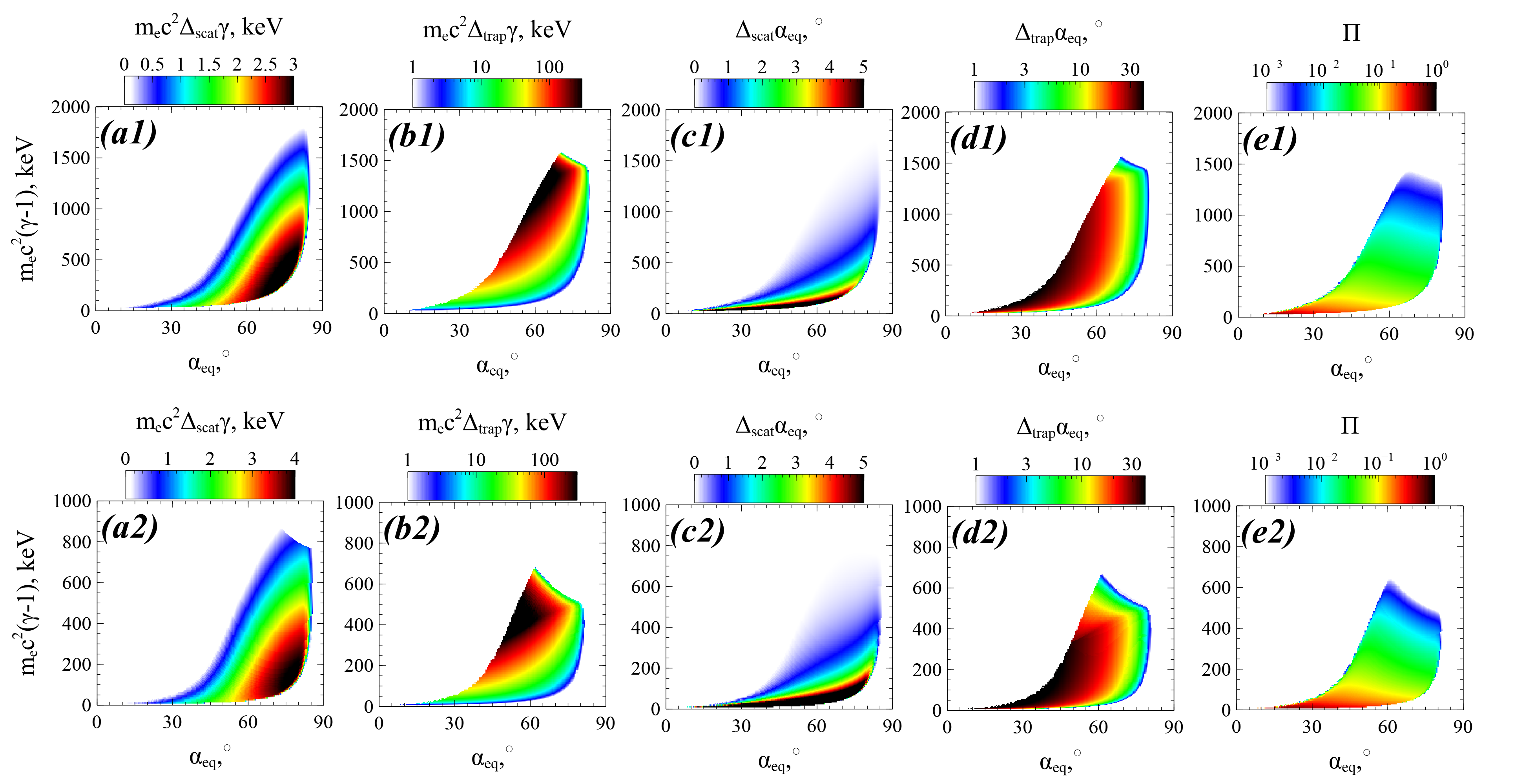
Figure 8: System characteristics for two field-aligned whistler-mode waves with the parameters as in Fig. 1: energy change due to scattering (a) and trapping (b), pitch-angle change due to scattering (c) and trapping (d), trapping probability (e).

Substituting characteristics from Figure 8 into map (21), we evaluate dynamics of resonant electrons. Figure 9 shows a sample trajectory: energy and pitch-angle are plotted versus the number of iterations $k$ and versus time $t=\sum_{k}\tau_{b,k}(\gamma,\alpha_{eq})$. The trajectory obtained with the mapping technique contains all elements that can be found in the numerically integrated trajectory (compare with Fig. 2): energy decrease due to phase bunching and rare jumps due to phase trapping. Note that the bounce period is given by $\tau_{b}=4\int_{0}^{s_{\max}}ds/p$ with $p=m_{e}c^{2}\sqrt{1-\gamma-2I_{x}\Omega_{ce}(s)}$ and $2I_{x}\Omega_{ce}(s_{\max})=1-\gamma$. Any direct comparison of trajectories obtained via numerical integration and mapping technique is not possible due to significant randomization of resonant electron motion, i.e. trajectories in energy/pitch-angle plane for two test electrons can differ significantly even with small difference of initial electron phases (e.g., Shklyar, 1981; Le Queau & Roux, 1987; Albert, 2001). Thus, the verification of map (21) is mainly based on verification of Eqs. (3,18) (see Artemyev et al., 2015, 2016b; Vainchtein et al., 2018) and on verification of 1D analogs of this map (see Artemyev et al., 2020b).

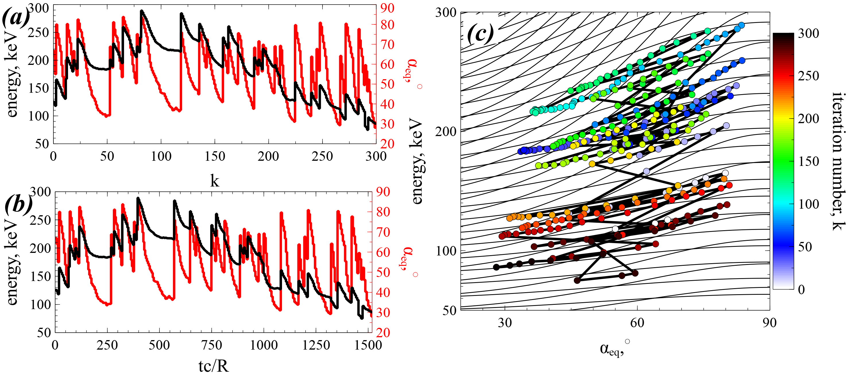
Figure 9: A sample trajectory obtained using map (21): energy and pitch-angle versus number of map iterations (a), energy and pitch-angle versus time (b), particle trajectory in the energy/pitch-angle space (c).

Using map (21), we can simulate the evolution of the electron distribution function as an ensemble of test trajectories. We start with the test simulation of electron spread in the energy/pitch-angle space. Four populations of electrons with small ranges of initial energy and pitch-angles are traced for $500$ interactions and their positions in energy/pitch-angle space are shown at six different times, see Fig. 10. White color shows the area of resonant wave-particle interaction (see Appendix B for a definition of this area and for technical details of map (21) application). Electrons of different initial populations quickly (already after $tc/R\sim 50$, i.e., $\sim 15$ resonant interactions) spread within a wide pitch-angle range, but are somehow separated in energy. After $tc/R\sim 300$ ($\sim 80$ resonant interactions) the populations fill large areas in energy/pitch-angle space and start overlapping. After $tc/R\sim 1000$ ($\sim 250$ resonant interactions) the entire energy/pitch-angle space is covered, and electrons from low energy populations (black and blue) reach high energies ($\sim 1$ MeV), whereas electrons from high-energy populations (red and magenta) decelerate with energy losses of several hundred keVs. Such fast phase mixing should result in spreading and smoothing of the electron phase space density.

Figure 10: Evolution of four electron populations modeled with map (21). Six moments of time are shown. White color shows the area of wave-particle nonlinear resonant interaction, see Appendix B.

To examine the evolution of the electron phase space density, we start with a power law distribution $f_{0}(\gamma,\alpha)=C\cdot\sin\alpha_{eq}\cdot(\gamma-1)^{-3}$ typical in the radiation belts, and fit this distribution by $2\cdot 10^{7}$ trajectories. There are $180\times 400$ pitch-angle/energy values, and $\sim 22600$ within the resonant area; for each value within the resonant area, we run $1000$ trajectories. Each trajectory is traced for 300 interactions with the map (21), and corresponding $\alpha_{eq}(k)$, $\gamma(k)$ profiles transferred to time series. Then, we recalculate the distribution from $f_{0}$ using phase space density conservation along the trajectories. Figure 11 shows three snapshots of the distribution $f(\alpha,\gamma)$ at different times (inserted panels show the low energy sub-interval). The rapid evolution of the distribution function results in phase space density flattening within the resonant region: there is an increase of high-energy/small pitch-angle phase space density and a decrease of low energy/large pitch-angle phase space density. During the simulation time, one electron can be trapped several times, i.e., most of particles circulate in the energy/pitch-angle space, because trappings bring them to the high energy region from which they then drift by bunching. Such a circulation also comprises successive trappings by two waves that bring electrons to the very high-energy region, whereas long periods of phase bunching without trappings can transport very energetic electrons to quite low energies. The last two phenomena are less frequent, and mixing of $\sim 1$ MeV electrons with $<100$ keV electrons is slower than mixing within energy localized domains.

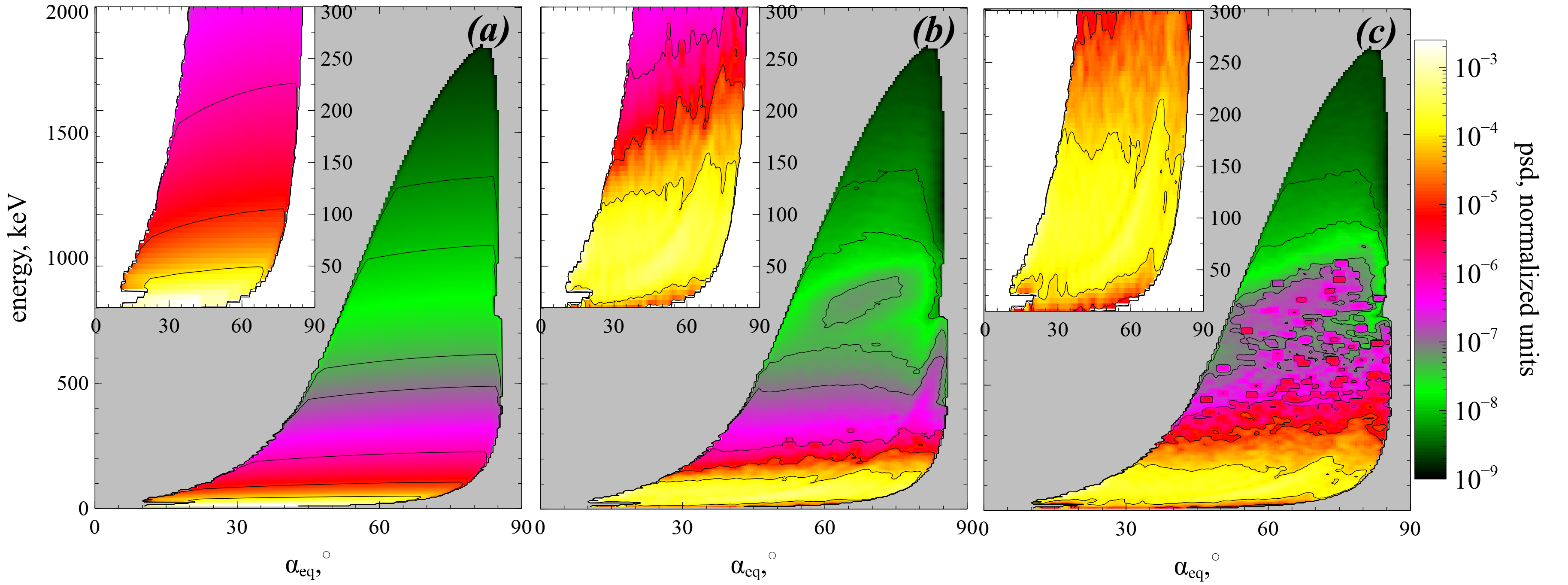
Figure 11: Evolution of electron distribution modeled with map (21). Three moments of time are shown: $tc/R=0$ (a), $tc/R=300$ (b), $tc/R=1000$ (c). The initial distribution $f_{0}(\gamma,\alpha)=C\cdot\sin\alpha_{eq}\cdot(\gamma-1)^{-3}$ in panel (a).

The general trend of the resonant electron transport in the energy/pitch-angle space is the reduction of phase space density gradients. In the presence of a single wave, such a gradient smoothing occurs along the resonant curves, $\gamma-\omega_{0}I_{0}={\rm const}$ (Artemyev et al., 2020b). In systems with two waves, the intersection of resonant curves $\gamma-\omega_{0}I_{0}={\rm const}$ and $\gamma-\omega_{1}I_{1}={\rm const}$ results in 2D gradient smoothing, i.e., we can expect a reduction of gradients in energy space after integration over pitch-angle. Figure 12 shows such electron acceleration: increase of high-energy population and decrease of low energy population that result in gradient smoothing. This is the typical evolution of the electron distribution due to resonant interaction with whistler-mode waves (see similar results for nonlinear (Vainchtein et al., 2018) and quasi-linear (Thorne et al., 2013; Li et al., 2014) simulations).

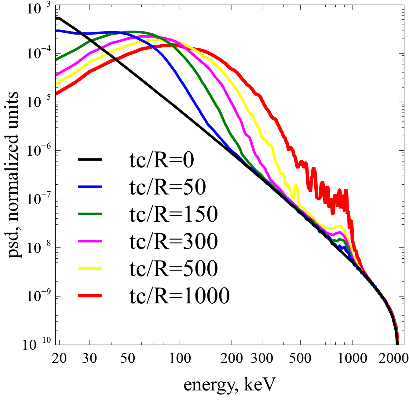
Figure 12: Pitch-angle integrated electron distribution, $\int_{0}^{\pi}\sin\alpha_{eq}\cdot psd(E,\alpha_{eq})d\alpha_{eq}$, from Fig. 11.

4 Discussion and conclusions

The proposed approach allows to investigate the long-term evolution of the electron distribution function in a system with nonlinear wave-particle interaction. This approach is based on the mapping technique that significantly simplifies electron trajectory integration by excluding from the consideration the main, adiabatic part of electron orbits and by focusing only on small intervals of resonant electron phase bunching and trapping. This approach is somewhat analogous to the Green function method proposed by (Furuya et al., 2008; Omura et al., 2015) and to the nonlinear kinetic equation proposed by (Artemyev et al., 2016b; Vainchtein et al., 2018). However, contrary to these other methods, the mapping does not require a very fine discretization of energy/pitch-angle space and it can easily be generalized to multi-wave systems. Resonances with different waves are very important for the destruction of the symmetry typical for the single wave system, where conservation of $(\gamma-\omega I)$ results in a reduced mixing in energy/pitch-angle space. Already, two waves with different characteristics are sufficient to produce a total mixing in energy/pitch-angle space (see Fig. 10) and a smoothing (reduction) of electron phase space density gradients (see Figure 12). The similar effect of fast mixing due to two independent resonances has been found in various dynamical systems with quite general properties (e.g. Gelfreich et al., 2011; Itin & Neishtadt, 2012).

Moreover, note that our simulations shown in Figures 9-12 are quite localized in time, since $R/c\sim 1000$ is about 100 s in the outer radiation belt ($L\sim 5$), and that this time period is much smaller than the characteristic time of evolution of any process typically modelled by quasi-linear theory (Thorne et al., 2013; Drozdov et al., 2015; Albert et al., 2016; Ma et al., 2016, 2018). Therefore, we extend the simulation interval to $tc/R=2.5\cdot 10^{4}$ ($\sim 40$ min) to show that this time scale is already sufficiently long to almost fully smooth gradients within $<1$ MeV, see Fig. 13. Generally, however, 40 minutes is a too long interval to keep whistler-mode wave activity at the same high level (although such long-living regions of intense waves are sometimes observed, see (Cully et al., 2008; Agapitov et al., 2015b; Cattell et al., 2015)).

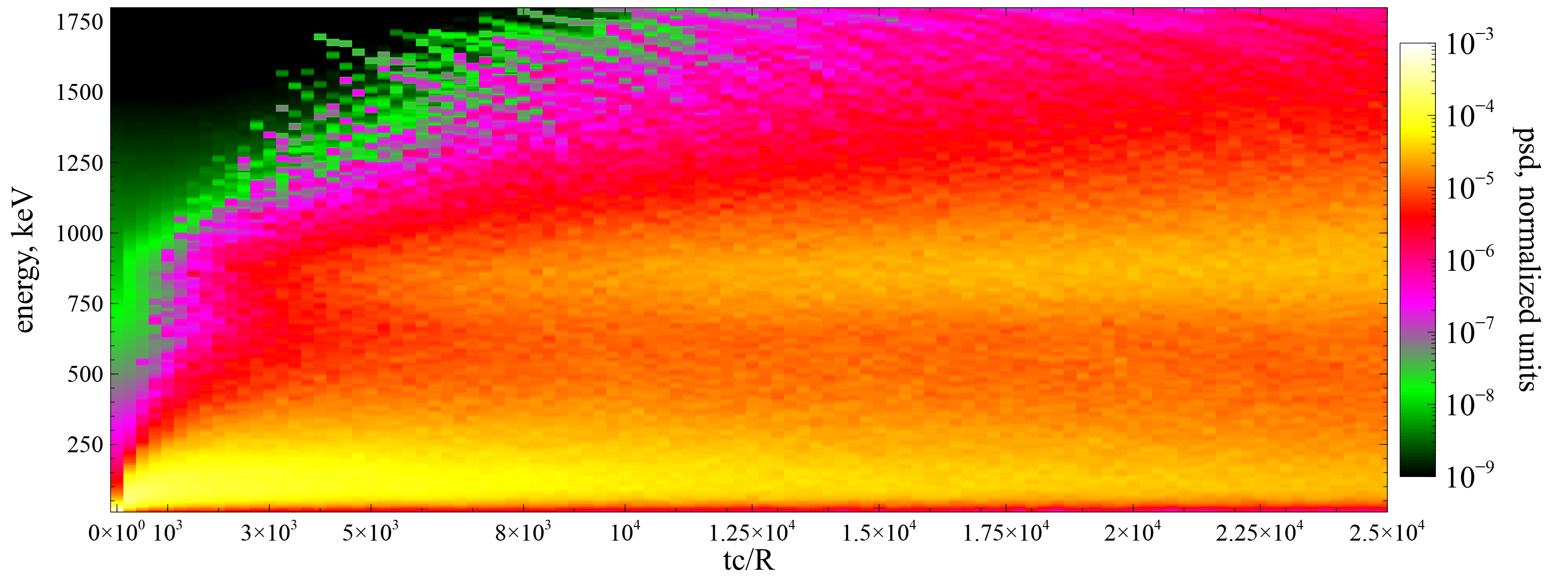
Figure 13: Evolution of pitch-angle integrated electron distribution, $\int_{0}^{\pi}\sin\alpha_{eq}\cdot psd(E,\alpha_{eq})d\alpha_{eq}$ in a long-term simulation.

Figure 8 shows energy/pitch-angle domains of nonlinear wave-particle interaction, and these domains are used for the simulation of the electron distribution function evolution (see Figures 10-13 and Appendix C). For simplicity, we assume that the boundary of these domains is impenetrable. However, additionally to nonlinear wave-particle interactions (phase bunching and phase trapping), there is also in reality some electron diffusion. This diffusion is finite everywhere in the energy/pitch-angle plane where there is an electron resonance with the whistler-mode wave. Thus, this diffusion would transport electrons across the boundary of the domains of nonlinear wave-particle interaction. The direction of this transport depends on the phase space density gradients. At low energies, the nonlinear wave-particle interaction results in phase space density decrease (see Fig. 13), and thus pitch-angle diffusion will bring new small-energy particles into these domains. At high energies, the nonlinear wave-particle interaction results in phase space density increase (see Fig. 13), and thus both energy and pitch-angle diffusion will try to spread this phase space density maximum. Such diffusion can be included into the map (21) as random energy and pitch-angle jumps with zero mean values and amplitudes given by the quasi-linear model (e.g., Albert, 2010). However, the diffusion is generally much weaker than nonlinear phase bunching and trapping, and the diffusion-driven evolution of the phase space density should mostly appear after nonlinear wave-particle interaction has already partly smoothed the initial phase space density gradients (Artemyev et al., 2019a).

The map (21) has been constructed for electron interaction with monochromatic waves (see Eq. (1)), whereas spacecraft observations in the Earth’s radiation belts often report about more complex wave field distributions, e.g., significant wave amplitude modulation (Tao et al., 2013; Santolík et al., 2014; Zhang et al., 2018, 2019), accompanied by fast, strong, and random variations of wave frequency and phase (Zhang et al., 2020b, a), often resulting in the formation of almost independent short wave packets or sub-packets (Mourenas et al., 2018; Zhang et al., 2020a). Such a chaotization of wave fields is likely partly driven by currents of resonant electrons (Nunn et al., 2009; Demekhov, 2011; Katoh & Omura, 2011, 2016; Tao et al., 2017, 2020) and sideband instability (Nunn, 1986), as well as by the simultaneous excitation of at least two different waves with a significant frequency difference (Katoh & Omura, 2013; Crabtree et al., 2017; Zhang et al., 2020b). Since phase bunching is a local process, wave modulation cannot affect the theoretical model of energy and pitch-angle jumps due to bunching, but the inclusion of such a modulation into the 2-wave model map would require some probabilistic distribution of wave amplitudes within short wave packets. The situation is more complicated for phase trapping, which is nonlocal and depends on wave packet size and amplitude modulation within the packets (Mourenas et al., 2018). Test particle simulations demonstrate that wave modulation alone makes phase trapping less efficient for electron acceleration, but increases the probability of phase trapping (Kubota & Omura, 2018; Gan et al., 2020; Zhang et al., 2020a). Thus, an important further development of the mapping technique for nonlinear wave-particle interaction would require modifications of the phase trapping model.

To conclude, we have demonstrated the usefulness of the mapping technique for Hamiltonian systems describing nonlinear resonant interaction of charged particles and intense electromagnetic waves. We have shown that in systems with two (and more) waves, the resonant interaction destroys the symmetries of the single wave resonance and drives a rapid smoothing of particle phase space density gradients. The proposed approach appears very promising for the investigation of relativistic electron interaction with various intense whistler-mode waves and EMIC waves in the Earth’s radiation belts (Katoh & Omura, 2013; Mourenas et al., 2016a, b; Ma et al., 2017; He et al., 2020; Yu et al., 2020; Zhang et al., 2020b) or in the solar wind (Wilson et al., 2007, 2013; Krafft et al., 2013; Krafft & Volokitin, 2016; Tong et al., 2019; Roberg-Clark et al., 2019). It could be useful also for studying electron acceleration by simultaneous laser-driven plasma waves (Modena et al., 1995; Tikhonchuk, 2019), and electron precipitation driven by VLF waves generated by electron beams or antennas in space (Carlsten et al., 2019; Borovsky et al., 2020).

Appendix A

Equation (17) describes energy decrease due to phase bunching, and natural limitation of this equation is that $\gamma+\Delta\gamma$ should be larger than one; or, alternatively, $I_{x}+(m_{e}c^{2}/\omega)\Delta\gamma$ should be larger than zero. This effect of drift asymmetry, i.e. absence of electron drift to negative $I_{x}$, has been noticed by Lundin & Shkliar (1977) who showed that for very small $I_{x}$ the phase bunching change the drift direction. This effect is called anomalous phase bunching (Kitahara & Katoh, 2019; Grach & Demekhov, 2020; Gan et al., 2020) and basically consists in positive $I_{x}$ (and $\gamma$) changes due to bunching at very small $I_{x}$. Theoretically, the parametrical boundary of anomalous bunching in energy/pitch-angle space is determined by $I_{x}<I_{x}^{*}$ with $I_{x}^{*}$ scaling as $(B_{w}/B_{0})^{2/3}$. Let us derive this scaling, but leave the more detailed consideration of small $I_{x}$ phase bunching to further consideration. We start with Eq. (LABEL:eq05) written for a single wave

$$H_{I}=-\omega I+m_{e}c^{2}\gamma+\sqrt{\frac{{2I\Omega_{ce}}}{{m_{e}c^{2}}}}\frac{e}{\gamma}\frac{{B_{w}}}{{k}}\sin\varphi,\;\;\;\;\gamma=\sqrt{1+\frac{{\left({P+kI}\right)^{2}}}{{m_{e}^{2}c^{2}}}+\frac{{2I\Omega_{ce}}}{{m_{e}c^{2}}}}$$ (22)

Hamiltonian equations for $I$ and $\varphi$ take the form:

$$\dot{I}=-\sqrt{\frac{{2I\Omega_{ce}}}{{m_{e}c^{2}}}}\frac{{eB_{w}}}{{k\gamma}}\sin\varphi,\quad\dot{\varphi}=\frac{{k^{2}}}{{\gamma m_{e}}}\left({I-I_{R}}\right)+\sqrt{\frac{{\Omega_{ce}}}{{2Im_{e}c^{2}}}}\frac{{eB_{w}}}{{k\gamma}}\sin\varphi$$ (23)

where $I_{R}=(\gamma\omega m_{e}-P)/k$ is the solution of $\partial H/\partial I=0$ equation for $B_{w}=0$. Equation (23) describes fast phase rotation (with frequency $k^{2}(I-I_{R})/\gamma m_{e}$) and $I,\varphi$ evolution driven by much weaker wave force $\sim B_{w}/B_{0}$. Until $I$ (and $I_{R}$) are sufficiently large to keep this time separation, we can apply the theory of phase bunching resulting in Eq. (17). However, let us consider small $I,I_{R}$ values. We introduce a small parameter $\varepsilon=B_{w}/B_{0}$ and normalized $(\tilde{I},\tilde{I}_{R})=(I,I_{R})/\varepsilon^{\beta}$:

$$\frac{{d\tilde{I}}}{{dt}}=-\sqrt{\frac{{2\tilde{I}\Omega_{ce}}}{{m_{e}c^{2}}}}\frac{{eB_{0}}}{{k\gamma}}\varepsilon^{1-\beta/2}\sin\varphi,\quad\frac{{d\varphi}}{{dt}}=\frac{{k^{2}\varepsilon^{\beta}}}{{\gamma m_{e}}}\left({\tilde{I}-\tilde{I}_{R}}\right)+\sqrt{\frac{{\Omega_{ce}}}{{2\tilde{I}m_{e}c^{2}}}}\frac{{eB_{0}}}{{k\gamma}}\varepsilon^{1-\beta/2}\sin\varphi$$ (24)

Introducing slow time $\tau=t\varepsilon^{1-\beta/2}$, we obtain

$$\frac{{d\tilde{I}}}{{d\tau}}=-\sqrt{\frac{{2\tilde{I}\Omega_{ce}}}{{m_{e}c^{2}}}}\frac{{eB_{0}}}{{k\gamma}}\sin\varphi,\quad\frac{{d\varphi}}{{d\tau}}=\frac{{k^{2}}}{{\gamma m_{e}}}\left({\tilde{I}-\tilde{I}_{R}}\right)\varepsilon^{3\beta/2-1}+\sqrt{\frac{{\Omega_{ce}}}{{2\tilde{I}m_{e}c^{2}}}}\frac{{eB_{0}}}{{k\gamma}}\sin\varphi$$ (25)

Thus, for $\beta=2/3$ Eqs. (25) lose the small parameter, and $\tilde{I},\varphi$ would change with the same rate. Then the applicability of equations of the phase bunching theory breaks, and a new model for $\Delta I$ (or $\Delta\gamma$, $\Delta I_{x}$) is required. $\beta=2/3$ gives the threshold value for $I_{x}\sim I\sim(B_{w}/B_{0})^{\beta}$.

Appendix B

Figure 8 shows that there are certain domains in the energy/pitch-angle space where electrons resonate with whistler wave nonlinearly. Thus, simulation of resonant electron dynamics should be within these domains. Figure 14(b) shows the largest domain that cover all energies and pitch-angles where electrons experience phase bunching. The phase bunching results in energy/pitch-angle change and electron drifts within the domain. Important property of the domain boundary is that $\Delta_{scat}\gamma$ tends there to zero as $\sim(I-I_{boundary})^{4/3}$ where $I$ and $I_{boundary}$ are values of moment and it’s boundary value (Artemyev et al., 2019a), i.e. $\Delta\gamma$ drops to zero at the domain boundary and no particles should leave this domain (in absence of diffusion that is characterized by a finite diffusion coefficient within the entire energy/pitch-angle space). As $\Delta_{scat}\gamma$ has been derived numerically, there are possible fluctuations making $\Delta_{scat}\gamma$ finite at the boundary. Thus, distribution $\Delta\gamma(E,\alpha_{eq})$ should be corrected to set $\Delta_{scat}\gamma=0$ at the domain boundary. Moreover, if during the simulation resonant electrons escape from the domain of phase bunching (e.g., because of numerical effects), these electrons should be returned into the domain (e.g., reflecting them back from the boundary on the same $\Delta_{scat}\gamma$). Note that this procedure is required only in the absence of particle diffusion.

Figure 14: Domains in energy/pitch-angle space with: positive probability of trapping (a), a finite phase bunching energy/pitch-angle change (b), positions of release from the trapping (c). Red curve shows boundary of (b) domain.

The domain of a finite trapping probability is smaller than the bunching domain (see Fig. 14(a)). Again, the probability of trapping tends to zero at the phase bunching domain boundary as $\Pi\sim(I-I_{boundary})^{1/3}$ (Artemyev et al., 2019a), and $\Pi$ should be set equal to zero on this boundary even if numerical fluctuations of $\Pi$ evaluation give some finite value. Of course, there are no regions with $\Pi>0$ outside the phase bunching domain.

Release of trapped electrons from the resonance also should be within the phase bunching domain (see Fig. 14(c)). Numerical errors put some release locations outside this domain; the trapping variation $\Delta_{trap}\gamma$ should be corrected to move the release locations within the domain. This guarantees that for each energy/pitch-angle within the phase bunching domain we would have incoming and outcoming phase space flows.

References

- Agapitov et al. (2013) Agapitov, O. V., Artemyev, A., Krasnoselskikh, V., Khotyaintsev, Y. V., Mourenas, D., Breuillard, H., Balikhin, M. & Rolland, G. 2013 Statistics of whistler mode waves in the outer radiation belt: Cluster STAFF-SA measurements. J. Geophys. Res. 118, 3407–3420.
- Agapitov et al. (2014) Agapitov, O. V., Artemyev, A., Mourenas, D., Krasnoselskikh, V., Bonnell, J., Le Contel, O., Cully, C. M. & Angelopoulos, V. 2014 The quasi-electrostatic mode of chorus waves and electron nonlinear acceleration. J. Geophys. Res. 119, 1606–1626.
- Agapitov et al. (2015a) Agapitov, O. V., Artemyev, A. V., Mourenas, D., Mozer, F. S. & Krasnoselskikh, V. 2015a Empirical model of lower band chorus wave distribution in the outer radiation belt. J. Geophys. Res. 120, 10.
- Agapitov et al. (2015b) Agapitov, O. V., Artemyev, A. V., Mourenas, D., Mozer, F. S. & Krasnoselskikh, V. 2015b Nonlinear local parallel acceleration of electrons through Landau trapping by oblique whistler mode waves in the outer radiation belt. Geophys. Res. Lett. 42, 10.
- Albert (1993) Albert, J. M. 1993 Cyclotron resonance in an inhomogeneous magnetic field. Physics of Fluids B 5, 2744–2750.
- Albert (2001) Albert, J. M. 2001 Comparison of pitch angle diffusion by turbulent and monochromatic whistler waves. J. Geophys. Res. 106, 8477–8482.
- Albert (2010) Albert, J. M. 2010 Diffusion by one wave and by many waves. J. Geophys. Res. 115, 0.
- Albert et al. (2016) Albert, J. M., Starks, M. J., Horne, R. B., Meredith, N. P. & Glauert, S. A. 2016 Quasi-linear simulations of inner radiation belt electron pitch angle and energy distributions. Geophys. Res. Lett. 43, 2381–2388.
- Albert et al. (2013) Albert, J. M., Tao, X. & Bortnik, J. 2013 Aspects of Nonlinear Wave-Particle Interactions. In Dynamics of the Earth’s Radiation Belts and Inner Magnetosphere (ed. D. Summers, I. U. Mann, D. N. Baker & M. Schulz).
- Allanson et al. (2020) Allanson, O., Watt, C. E. J., Ratcliffe, H., Allison, H. J., Meredith, N. P., Bentley, S. N., Ross, J. P. J. & Glauert, S. A. 2020 Particle-in-Cell Experiments Examine Electron Diffusion by Whistler-Mode Waves: 2. Quasi-Linear and Nonlinear Dynamics. Journal of Geophysical Research (Space Physics) 125 (7), e27949.
- Andronov & Trakhtengerts (1964) Andronov, A. A. & Trakhtengerts, V. Y. 1964 Kinetic instability of the Earth’s outer radiation belt. Geomagnetism and Aeronomy 4, 233–242.
- Arnold et al. (2006) Arnold, V. I., Kozlov, V. V. & Neishtadt, A. I. 2006 Mathematical Aspects of Classical and Celestial Mechanics, 3rd edn. New York: Springer-Verlag.
- Artemyev et al. (2016a) Artemyev, A. V., Agapitov, O., Mourenas, D., Krasnoselskikh, V., Shastun, V. & Mozer, F. 2016a Oblique Whistler-Mode Waves in the Earth’s Inner Magnetosphere: Energy Distribution, Origins, and Role in Radiation Belt Dynamics. Space Sci. Rev. 200 (1-4), 261–355.
- Artemyev et al. (2018a) Artemyev, A. V., Neishtadt, A. I., Vainchtein, D. L., Vasiliev, A. A., Vasko, I. Y. & Zelenyi, L. M. 2018a Trapping (capture) into resonance and scattering on resonance: Summary of results for space plasma systems. Communications in Nonlinear Science and Numerical Simulations 65, 111–160.
- Artemyev et al. (2019a) Artemyev, A. V., Neishtadt, A. I. & Vasiliev, A. A. 2019a Kinetic equation for nonlinear wave-particle interaction: Solution properties and asymptotic dynamics. Physica D Nonlinear Phenomena 393, 1–8, arXiv: 1809.03743.
- Artemyev et al. (2020a) Artemyev, A. V., Neishtadt, A. I. & Vasiliev, A. A. 2020a A Map for Systems with Resonant Trappings and Scatterings. Regular and Chaotic Dynamics 25 (1), 2–10.
- Artemyev et al. (2020b) Artemyev, A. V., Neishtadt, A. I. & Vasiliev, A. A. 2020b Mapping for nonlinear electron interaction with whistler-mode waves. Physics of Plasmas 27 (4), 042902, arXiv: 1911.11459.
- Artemyev et al. (2016b) Artemyev, A. V., Neishtadt, A. I., Vasiliev, A. A. & Mourenas, D. 2016b Kinetic equation for nonlinear resonant wave-particle interaction. Physics of Plasmas 23 (9), 090701.
- Artemyev et al. (2017) Artemyev, A. V., Neishtadt, A. I., Vasiliev, A. A. & Mourenas, D. 2017 Probabilistic approach to nonlinear wave-particle resonant interaction. Phys. Rev. E 95 (2), 023204.
- Artemyev et al. (2018b) Artemyev, A. V., Neishtadt, A. I., Vasiliev, A. A. & Mourenas, D. 2018b Long-term evolution of electron distribution function due to nonlinear resonant interaction with whistler mode waves. Journal of Plasma Physics 84, 905840206.
- Artemyev et al. (2013) Artemyev, A. V., Vasiliev, A. A., Mourenas, D., Agapitov, O. & Krasnoselskikh, V. 2013 Nonlinear electron acceleration by oblique whistler waves: Landau resonance vs. cyclotron resonance. Physics of Plasmas 20, 122901.
- Artemyev et al. (2014a) Artemyev, A. V., Vasiliev, A. A., Mourenas, D., Agapitov, O., Krasnoselskikh, V., Boscher, D. & Rolland, G. 2014a Fast transport of resonant electrons in phase space due to nonlinear trapping by whistler waves. Geophys. Res. Lett. 41, 5727–5733.
- Artemyev et al. (2014b) Artemyev, A. V., Vasiliev, A. A., Mourenas, D., Agapitov, O. V. & Krasnoselskikh, V. V. 2014b Electron scattering and nonlinear trapping by oblique whistler waves: The critical wave intensity for nonlinear effects. Physics of Plasmas 21 (10), 102903.
- Artemyev et al. (2015) Artemyev, A. V., Vasiliev, A. A., Mourenas, D., Neishtadt, A. I., Agapitov, O. V. & Krasnoselskikh, V. 2015 Probability of relativistic electron trapping by parallel and oblique whistler-mode waves in Earth’s radiation belts. Physics of Plasmas 22 (11), 112903.
- Artemyev et al. (2019b) Artemyev, A. V., Vasiliev, A. A. & Neishtadt, A. I. 2019b Charged particle nonlinear resonance with localized electrostatic wave-packets. Communications in Nonlinear Science and Numerical Simulations 72, 392–406.
- Balikhin et al. (1997) Balikhin, M. A., de Wit, T. D., Alleyne, H. S. C. K., Woolliscroft, L. J. C., Walker, S. N., Krasnosel’skikh, V., Mier-Jedrzejeowicz, W. A. C. & Baumjohann, W. 1997 Experimental determination of the dispersion of waves observed upstream of a quasi-perpendicular shock. Geophys. Res. Lett. 24, 787–790.
- Bell (1984) Bell, T. F. 1984 The nonlinear gyroresonance interaction between energetic electrons and coherent VLF waves propagating at an arbitrary angle with respect to the earth’s magnetic field. J. Geophys. Res. 89, 905–918.
- Benkadda et al. (1996) Benkadda, S., Sen, A. & Shklyar, D. R. 1996 Chaotic dynamics of charged particles in the field of two monochromatic waves in a magnetized plasma. Chaos 6 (3), 451–460.
- Borovsky et al. (2020) Borovsky, J. E., Delzanno, G. L., Dors, E. E., Thomsen, M. F., Sanchez, E. R., Henderson, M. G., Marshall, R. A., Gilchrist, B. E., Miars, G., Carlsten, B. E., Storms, S. A., Holloway, M. A. & Nguyen, D. 2020 Solving the auroral-arc-generator question by using an electron beam to unambiguously connect critical magnetospheric measurements to auroral images. Journal of Atmospheric and Solar-Terrestrial Physics 206, 105310.
- Camporeale & Zimbardo (2015) Camporeale, E. & Zimbardo, G. 2015 Wave-particle interactions with parallel whistler waves: Nonlinear and time-dependent effects revealed by particle-in-cell simulations. Physics of Plasmas 22 (9), 092104, arXiv: 1412.3229.
- Carlsten et al. (2019) Carlsten, B. E., Colestock, P. L., Cunningham, G. S., Delzanno, G. L., Dors, E. E., Holloway, M. A., Jeffery, C. A., Lewellen, J. W., Marksteiner, Q. R., Nguyen, D. C., Reeves, G. D. & Shipman, K. A. 2019 Radiation-Belt Remediation Using Space-Based Antennas and Electron Beams. IEEE Transactions on Plasma Science 47 (5), 2045–2063.
- Cattell et al. (2008) Cattell, C., Wygant, J. R., Goetz, K., Kersten, K., Kellogg, P. J., von Rosenvinge, T., Bale, S. D., Roth, I., Temerin, M., Hudson, M. K., Mewaldt, R. A., Wiedenbeck, M., Maksimovic, M., Ergun, R., Acuna, M. & Russell, C. T. 2008 Discovery of very large amplitude whistler-mode waves in Earth’s radiation belts. Geophys. Res. Lett. 35, 1105.
- Cattell et al. (2015) Cattell, C. A., Breneman, A. W., Thaller, S. A., Wygant, J. R., Kletzing, C. A. & Kurth, W. S. 2015 Van Allen Probes observations of unusually low frequency whistler mode waves observed in association with moderate magnetic storms: Statistical study. Geophys. Res. Lett. 42, 7273–7281.
- Chaston et al. (2008) Chaston, C. C., Salem, C., Bonnell, J. W., Carlson, C. W., Ergun, R. E., Strangeway, R. J. & McFadden, J. P. 2008 The Turbulent Alfvénic Aurora. Physical Review Letters 100 (17), 175003.
- Chen et al. (2020) Chen, L., Breneman, A. W., Xia, Z. & Zhang, X.-j. 2020 Modeling of Bouncing Electron Microbursts Induced by Ducted Chorus Waves. Geophys. Res. Lett. 47 (17), e89400.
- Chen et al. (2019) Chen, L., Zhu, H. & Zhang, X. 2019 Wavenumber Analysis of EMIC Waves. Geophys. Res. Lett. 46 (11), 5689–5697.
- Chirikov (1979) Chirikov, B. V. 1979 A universal instability of many-dimensional oscillator systems. Physics Reports 52, 263–379.
- Crabtree et al. (2017) Crabtree, C., Tejero, E., Ganguli, G., Hospodarsky, G. B. & Kletzing, C. A. 2017 Bayesian spectral analysis of chorus subelements from the Van Allen Probes. Journal of Geophysical Research (Space Physics) 122 (6), 6088–6106.
- Cully et al. (2011) Cully, C. M., Angelopoulos, V., Auster, U., Bonnell, J. & Le Contel, O. 2011 Observational evidence of the generation mechanism for rising-tone chorus. Geophys. Res. Lett. 38, 1106.
- Cully et al. (2008) Cully, C. M., Bonnell, J. W. & Ergun, R. E. 2008 THEMIS observations of long-lived regions of large-amplitude whistler waves in the inner magnetosphere. Geophys. Res. Lett. 35, 17.
- Demekhov (2011) Demekhov, A. G. 2011 Generation of VLF emissions with the increasing and decreasing frequency in the magnetosperic cyclotron maser in the backward wave oscillator regime. Radiophysics and Quantum Electronics 53, 609–622.
- Demekhov et al. (2009) Demekhov, A. G., Trakhtengerts, V. Y., Rycroft, M. & Nunn, D. 2009 Efficiency of electron acceleration in the Earth’s magnetosphere by whistler mode waves. Geomagnetism and Aeronomy 49, 24–29.
- Demekhov et al. (2006) Demekhov, A. G., Trakhtengerts, V. Y., Rycroft, M. J. & Nunn, D. 2006 Electron acceleration in the magnetosphere by whistler-mode waves of varying frequency. Geomagnetism and Aeronomy 46, 711–716.
- Drozdov et al. (2015) Drozdov, A. Y., Shprits, Y. Y., Orlova, K. G., Kellerman, A. C., Subbotin, D. A., Baker, D. N., Spence, H. E. & Reeves, G. D. 2015 Energetic, relativistic, and ultrarelativistic electrons: Comparison of long-term VERB code simulations with Van Allen Probes measurements. J. Geophys. Res. 120, 3574–3587.
- Drummond & Pines (1962) Drummond, W. E. & Pines, D. 1962 Nonlinear stability of plasma oscillations. Nuclear Fusion Suppl. 3, 1049–1058.
- Foster et al. (2014) Foster, J. C., Erickson, P. J., Baker, D. N., Claudepierre, S. G., Kletzing, C. A., Kurth, W., Reeves, G. D., Thaller, S. A., Spence, H. E., Shprits, Y. Y. & Wygant, J. R. 2014 Prompt energization of relativistic and highly relativistic electrons during a substorm interval: Van Allen Probes observations. Geophys. Res. Lett. 41, 20–25.
- Furuya et al. (2008) Furuya, N., Omura, Y. & Summers, D. 2008 Relativistic turning acceleration of radiation belt electrons by whistler mode chorus. J. Geophys. Res. 113, 4224.
- Gan et al. (2020) Gan, L., Li, W., Ma, Q., Albert, J. M., Artemyev, A. V. & Bortnik, J. 2020 Nonlinear Interactions Between Radiation Belt Electrons and Chorus Waves: Dependence on Wave Amplitude Modulation. Geophys. Res. Lett. 47 (4), e85987.
- Gelfreich et al. (2011) Gelfreich, V., Rom-Kedar, V., Shah, K. & Turaev, D. 2011 Robust Exponential Acceleration in Time-Dependent Billiards. Phys. Rev. Lett. 106 (7), 074101.
- Grach & Demekhov (2018) Grach, V. S. & Demekhov, A. G. 2018 Resonance Interaction of Relativistic Electrons with Ion-Cyclotron Waves. I. Specific Features of the Nonlinear Interaction Regimes. Radiophysics and Quantum Electronics 60 (12), 942–959.
- Grach & Demekhov (2020) Grach, V. S. & Demekhov, A. G. 2020 Precipitation of Relativistic Electrons Under Resonant Interaction With Electromagnetic Ion Cyclotron Wave Packets. Journal of Geophysical Research (Space Physics) 125 (2), e27358.
- He et al. (2020) He, Z., Yan, Q., Zhang, X., Yu, J., Ma, Y., Cao, Y. & Cui, J. 2020 Precipitation loss of radiation belt electrons by two-band plasmaspheric hiss waves. Journal of Geophysical Research: Space Physics p. e2020JA028157.
- Hiraga & Omura (2020) Hiraga, R. & Omura, Y. 2020 Acceleration mechanism of radiation belt electrons through interaction with multi-subpacket chorus waves. Earth, Planets, and Space 72 (1), 21.
- Hsieh et al. (2020) Hsieh, Y.-K., Kubota, Y. & Omura, Y. 2020 Nonlinear evolution of radiation belt electron fluxes interacting with oblique whistler mode chorus emissions. Journal of Geophysical Research: Space Physics p. e2019JA027465, e2019JA027465 2019JA027465, arXiv: https://agupubs.onlinelibrary.wiley.com/doi/pdf/10.1029/2019JA027465.
- Hsieh & Omura (2017) Hsieh, Y.-K. & Omura, Y. 2017 Nonlinear dynamics of electrons interacting with oblique whistler mode chorus in the magnetosphere. J. Geophys. Res. 122, 675–694.
- Hsieh & Omura (2017) Hsieh, Y.-K. & Omura, Y. 2017 Study of wave-particle interactions for whistler mode waves at oblique angles by utilizing the gyroaveraging method. Radio Science 52 (10), 1268–1281, 2017RS006245.
- Itin & Neishtadt (2012) Itin, A. P. & Neishtadt, A. I. 2012 Fermi acceleration in time-dependent rectangular billiards due to multiple passages through resonances. Chaos 22 (2), 026119, arXiv: 1112.3472.
- Itin et al. (2000) Itin, A. P., Neishtadt, A. I. & Vasiliev, A. A. 2000 Captures into resonance and scattering on resonance in dynamics of a charged relativistic particle in magnetic field and electrostatic wave. Physica D: Nonlinear Phenomena 141, 281–296.
- Karimabadi et al. (1990) Karimabadi, H., Akimoto, K., Omidi, N. & Menyuk, C. R. 1990 Particle acceleration by a wave in a strong magnetic field - Regular and stochastic motion. Physics of Fluids B 2, 606–628.
- Karpman (1974) Karpman, V. I. 1974 Nonlinear Effects in the ELF Waves Propagating along the Magnetic Field in the Magnetosphere. Space Sci. Rev. 16, 361–388.
- Katoh (2014) Katoh, Y. 2014 A simulation study of the propagation of whistler-mode chorus in the Earth’s inner magnetosphere. Earth, Planets, and Space 66, 6.
- Katoh & Omura (2011) Katoh, Y. & Omura, Y. 2011 Amplitude dependence of frequency sweep rates of whistler mode chorus emissions. J. Geophys. Res. 116, 7201.
- Katoh & Omura (2013) Katoh, Y. & Omura, Y. 2013 Effect of the background magnetic field inhomogeneity on generation processes of whistler-mode chorus and broadband hiss-like emissions. J. Geophys. Res. 118, 4189–4198.
- Katoh & Omura (2016) Katoh, Y. & Omura, Y. 2016 Electron hybrid code simulation of whistler-mode chorus generation with real parameters in the Earth’s inner magnetosphere. Earth, Planets, and Space 68 (1), 192.
- Kennel & Engelmann (1966) Kennel, C. F. & Engelmann, F. 1966 Velocity Space Diffusion from Weak Plasma Turbulence in a Magnetic Field. Physics of Fluids 9, 2377–2388.
- Kersten et al. (2014) Kersten, T., Horne, R. B., Glauert, S. A., Meredith, N. P., Fraser, B. J. & Grew, R. S. 2014 Electron losses from the radiation belts caused by EMIC waves. J. Geophys. Res. 119, 8820–8837.
- Khazanov et al. (2013) Khazanov, G. V., Tel’nikhin, A. A. & Kronberg, T. K. 2013 Radiation belt electron dynamics driven by large-amplitude whistlers. Journal of Geophysical Research (Space Physics) 118 (10), 6397–6404.
- Khazanov et al. (2014) Khazanov, G. V., Tel’nikhin, A. A. & Kronberg, T. K. 2014 Stochastic electron motion driven by space plasma waves. Nonlinear Processes in Geophysics 21 (1), 61–85.
- Kitahara & Katoh (2019) Kitahara, M. & Katoh, Y. 2019 Anomalous Trapping of Low Pitch Angle Electrons by Coherent Whistler Mode Waves. J. Geophys. Res. 124 (7), 5568–5583.
- Kletzing et al. (2013) Kletzing, C. A., Kurth, W. S., Acuna, M., MacDowall, R. J., Torbert, R. B., Averkamp, T., Bodet, D., Bounds, S. R., Chutter, M., Connerney, J., Crawford, D., Dolan, J. S., Dvorsky, R., Hospodarsky, G. B., Howard, J., Jordanova, V., Johnson, R. A., Kirchner, D. L., Mokrzycki, B., Needell, G., Odom, J., Mark, D., Pfaff, R., Phillips, J. R., Piker, C. W., Remington, S. L., Rowland, D., Santolik, O., Schnurr, R., Sheppard, D., Smith, C. W., Thorne, R. M. & Tyler, J. 2013 The Electric and Magnetic Field Instrument Suite and Integrated Science (EMFISIS) on RBSP. Space Sci. Rev. 179, 127–181.
- Krafft & Volokitin (2016) Krafft, C. & Volokitin, A. S. 2016 Electron Acceleration by Langmuir Waves Produced by a Decay Cascade. ApJ 821, 99.
- Krafft et al. (2013) Krafft, C., Volokitin, A. S. & Krasnoselskikh, V. V. 2013 Interaction of Energetic Particles with Waves in Strongly Inhomogeneous Solar Wind Plasmas. ApJ 778, 111.
- Kubota & Omura (2017) Kubota, Y. & Omura, Y. 2017 Rapid precipitation of radiation belt electrons induced by EMIC rising tone emissions localized in longitude inside and outside the plasmapause. Journal of Geophysical Research (Space Physics) 122 (1), 293–309.
- Kubota & Omura (2018) Kubota, Y. & Omura, Y. 2018 Nonlinear Dynamics of Radiation Belt Electrons Interacting With Chorus Emissions Localized in Longitude. Journal of Geophysical Research (Space Physics) 123, 4835–4857.
- Kubota et al. (2015) Kubota, Y., Omura, Y. & Summers, D. 2015 Relativistic electron precipitation induced by EMIC-triggered emissions in a dipole magnetosphere. Journal of Geophysical Research (Space Physics) 120 (6), 4384–4399.
- Kuzichev et al. (2019) Kuzichev, I. V., Vasko, I. Y., Rualdo Soto-Chavez, A., Tong, Y., Artemyev, A. V., Bale, S. D. & Spitkovsky, A. 2019 Nonlinear Evolution of the Whistler Heat Flux Instability. ApJ 882 (2), 81, arXiv: 1907.04878.
- Le Queau & Roux (1987) Le Queau, D. & Roux, A. 1987 Quasi-monochromatic wave-particle interactions in magnetospheric plasmas. Sol. Phys. 111, 59–80.
- Leoncini et al. (2018) Leoncini, X., Vasiliev, A. & Artemyev, A. 2018 Resonance controlled transport in phase space. Physica D Nonlinear Phenomena 364, 22–26.
- Lerche (1968) Lerche, I. 1968 Quasilinear Theory of Resonant Diffusion in a Magneto-Active, Relativistic Plasma. Physics of Fluids 11.
- Li et al. (2016) Li, W., Santolik, O., Bortnik, J., Thorne, R. M., Kletzing, C. A., Kurth, W. S. & Hospodarsky, G. B. 2016 New chorus wave properties near the equator from Van Allen Probes wave observations. Geophys. Res. Lett. 43, 4725–4735.
- Li et al. (2014) Li, W., Thorne, R. M., Ma, Q., Ni, B., Bortnik, J., Baker, D. N., Spence, H. E., Reeves, G. D., Kanekal, S. G., Green, J. C., Kletzing, C. A., Kurth, W. S., Hospodarsky, G. B., Blake, J. B., Fennell, J. F. & Claudepierre, S. G. 2014 Radiation belt electron acceleration by chorus waves during the 17 March 2013 storm. J. Geophys. Res. 119, 4681–4693.
- Lichtenberg & Lieberman (1983) Lichtenberg, A. J. & Lieberman, M. A. 1983 Regular and stochastic motion.
- Lundin & Shkliar (1977) Lundin, B. V. & Shkliar, D. R. 1977 Interaction of electrons with low transverse velocities with VLF waves in an inhomogeneous plasma. Geomagnetism and Aeronomy 17, 246–251.
- Lyons & Williams (1984) Lyons, L. R. & Williams, D. J. 1984 Quantitative aspects of magnetospheric physics..
- Ma et al. (2018) Ma, Q., Li, W., Bortnik, J., Thorne, R. M., Chu, X., Ozeke, L. G., Reeves, G. D., Kletzing, C. A., Kurth, W. S., Hospodarsky, G. B., Engebretson, M. J., Spence, H. E., Baker, D. N., Blake, J. B., Fennell, J. F. & Claudepierre, S. G. 2018 Quantitative Evaluation of Radial Diffusion and Local Acceleration Processes During GEM Challenge Events. Journal of Geophysical Research (Space Physics) 123 (3), 1938–1952.
- Ma et al. (2016) Ma, Q., Li, W., Thorne, R. M., Nishimura, Y., Zhang, X.-J., Reeves, G. D., Kletzing, C. A., Kurth, W. S., Hospodarsky, G. B., Henderson, M. G., Spence, H. E., Baker, D. N., Blake, J. B., Fennell, J. F. & Angelopoulos, V. 2016 Simulation of energy-dependent electron diffusion processes in the Earth’s outer radiation belt. J. Geophys. Res. 121, 4217–4231.
- Ma et al. (2017) Ma, Q., Mourenas, D., Li, W., Artemyev, A. & Thorne, R. M. 2017 VLF waves from ground-based transmitters observed by the Van Allen Probes: Statistical model and effects on plasmaspheric electrons. Geophys. Res. Lett. 44, 6483–6491.
- Mauk et al. (2013) Mauk, B. H., Fox, N. J., Kanekal, S. G., Kessel, R. L., Sibeck, D. G. & Ukhorskiy, A. 2013 Science Objectives and Rationale for the Radiation Belt Storm Probes Mission. Space Sci. Rev. 179, 3–27.
- Mauk et al. (2017) Mauk, B. H., Haggerty, D. K., Paranicas, C., Clark, G., Kollmann, P., Rymer, A. M., Bolton, S. J., Levin, S. M., Adriani, A., Allegrini, F., Bagenal, F., Bonfond, B., Connerney, J. E. P., Gladstone, G. R., Kurth, W. S., McComas, D. J. & Valek, P. 2017 Discrete and broadband electron acceleration in Jupiter’s powerful aurora. Nature 549 (7670), 66–69.
- Menietti et al. (2012) Menietti, J. D., Shprits, Y. Y., Horne, R. B., Woodfield, E. E., Hospodarsky, G. B. & Gurnett, D. A. 2012 Chorus, ECH, and Z mode emissions observed at Jupiter and Saturn and possible electron acceleration. J. Geophys. Res. 117, A12214.
- Meredith et al. (2007) Meredith, N. P., Horne, R. B., Glauert, S. A. & Anderson, R. R. 2007 Slot region electron loss timescales due to plasmaspheric hiss and lightning-generated whistlers. J. Geophys. Res. 112, 8214.
- Millan & Thorne (2007) Millan, R. M. & Thorne, R. M. 2007 Review of radiation belt relativistic electron losses. Journal of Atmospheric and Solar-Terrestrial Physics 69, 362–377.
- Modena et al. (1995) Modena, A., Najmudin, Z., Dangor, A. E., Clayton, C. E., Marsh, K. A., Joshi, C., Malka, V., Darrow, C. B., Danson, C., Neely, D. & Walsh, F. N. 1995 Electron acceleration from the breaking of relativistic plasma waves. Nature 377 (6550), 606–608.
- Mourenas et al. (2012) Mourenas, D., Artemyev, A., Agapitov, O. & Krasnoselskikh, V. 2012 Acceleration of radiation belts electrons by oblique chorus waves. J. Geophys. Res. 117, 10212.
- Mourenas et al. (2015) Mourenas, D., Artemyev, A. V., Agapitov, O. V., Krasnoselskikh, V. & Mozer, F. S. 2015 Very oblique whistler generation by low-energy electron streams. J. Geophys. Res. 120, 3665–3683.
- Mourenas et al. (2016a) Mourenas, D., Artemyev, A. V., Agapitov, O. V., Mozer, F. S. & Krasnoselskikh, V. V. 2016a Equatorial electron loss by double resonance with oblique and parallel intense chorus waves. J. Geophys. Res. 121, 4498–4517.
- Mourenas et al. (2016b) Mourenas, D., Artemyev, A. V., Ma, Q., Agapitov, O. V. & Li, W. 2016b Fast dropouts of multi-MeV electrons due to combined effects of EMIC and whistler mode waves. Geophys. Res. Lett. 43 (9), 4155–4163.
- Mourenas et al. (2018) Mourenas, D., Zhang, X.-J., Artemyev, A. V., Angelopoulos, V., Thorne, R. M., Bortnik, J., Neishtadt, A. I. & Vasiliev, A. A. 2018 Electron Nonlinear Resonant Interaction With Short and Intense Parallel Chorus Wave Packets. J. Geophys. Res. 123, 4979–4999.
- Neishtadt (1999) Neishtadt, A. I. 1999 On Adiabatic Invariance in Two-Frequency Systems. in Hamiltonian Systems with Three or More Degrees of Freedom, ed. Simo C., NATO ASI Series C. Dordrecht: Kluwer Acad. Publ. 533, 193–213.
- Neishtadt (2014) Neishtadt, A. I. 2014 Averaging, passage through resonances, and capture into resonance in two-frequency systems. Russian Mathematical Surveys 69 (5), 771.
- Neishtadt & Vasiliev (2006) Neishtadt, A. I. & Vasiliev, A. A. 2006 Destruction of adiabatic invariance at resonances in slow fast Hamiltonian systems. Nuclear Instruments and Methods in Physics Research A 561, 158–165, arXiv: arXiv:nlin/0511050.
- Ni et al. (2016) Ni, B., Thorne, R. M., Zhang, X., Bortnik, J., Pu, Z., Xie, L., Hu, Z.-j., Han, D., Shi, R., Zhou, C. & Gu, X. 2016 Origins of the Earth’s Diffuse Auroral Precipitation. Space Sci. Rev. 200, 205–259.
- Nishimura et al. (2010) Nishimura, Y., Bortnik, J., Li, W., Thorne, R. M., Lyons, L. R., Angelopoulos, V., Mende, S. B., Bonnell, J. W., Le Contel, O., Cully, C., Ergun, R. & Auster, U. 2010 Identifying the Driver of Pulsating Aurora. Science 330, 81–84.
- Nunn (1986) Nunn, D. 1986 A nonlinear theory of sideband stability in ducted whistler mode waves. Planet. Space Sci. 34, 429–451.
- Nunn & Omura (2012) Nunn, D. & Omura, Y. 2012 A computational and theoretical analysis of falling frequency VLF emissions. J. Geophys. Res. 117, 8228.
- Nunn & Omura (2015) Nunn, D. & Omura, Y. 2015 A computational and theoretical investigation of nonlinear wave-particle interactions in oblique whistlers. J. Geophys. Res. 120, 2890–2911.
- Nunn et al. (2009) Nunn, D., Santolik, O., Rycroft, M. & Trakhtengerts, V. 2009 On the numerical modelling of VLF chorus dynamical spectra. Annales Geophysicae 27, 2341–2359.
- Omura et al. (2007) Omura, Y., Furuya, N. & Summers, D. 2007 Relativistic turning acceleration of resonant electrons by coherent whistler mode waves in a dipole magnetic field. J. Geophys. Res. 112, 6236.
- Omura et al. (2008) Omura, Y., Katoh, Y. & Summers, D. 2008 Theory and simulation of the generation of whistler-mode chorus. J. Geophys. Res. 113, 4223.
- Omura et al. (1991) Omura, Y., Matsumoto, H., Nunn, D. & Rycroft, M. J. 1991 A review of observational, theoretical and numerical studies of VLF triggered emissions. Journal of Atmospheric and Terrestrial Physics 53, 351–368.
- Omura et al. (2015) Omura, Y., Miyashita, Y., Yoshikawa, M., Summers, D., Hikishima, M., Ebihara, Y. & Kubota, Y. 2015 Formation process of relativistic electron flux through interaction with chorus emissions in the Earth’s inner magnetosphere. J. Geophys. Res. 120, 9545–9562.
- Omura et al. (2013) Omura, Y., Nunn, D. & Summers, D. 2013 Generation Processes of Whistler Mode Chorus Emissions: Current Status of Nonlinear Wave Growth Theory. In Dynamics of the Earth’s Radiation Belts and Inner Magnetosphere (ed. D. Summers, I. U. Mann, D. N. Baker & M. Schulz), pp. 243–254.
- Palmadesso (1972) Palmadesso, P. J. 1972 Resonance, Particle Trapping, and Landau Damping in Finite Amplitude Obliquely Propagating Waves. Physics of Fluids 15, 2006–2013.
- Roberg-Clark et al. (2019) Roberg-Clark, G. T., Agapitov, O., Drake, J. F. & Swisdak, M. 2019 Scattering of Energetic Electrons by Heat-flux-driven Whistlers in Flares. ApJ 887 (2), 190, arXiv: 1908.06481.
- Ryutov (1969) Ryutov, D. D. 1969 Quasilinear Relaxation of an Electron Beam in an Inhomogeneous Plasma. Soviet Journal of Experimental and Theoretical Physics 30, 131.
- Sagdeev et al. (1988) Sagdeev, R. Z., Usikov, D. A. & Zaslavsky, G. M. 1988 Nonlinear Physics. From the Pendulum to Turbulence and Chaos.
- Santolík et al. (2014) Santolík, O., Kletzing, C. A., Kurth, W. S., Hospodarsky, G. B. & Bounds, S. R. 2014 Fine structure of large-amplitude chorus wave packets. Geophys. Res. Lett. 41, 293–299.
- Santolík et al. (2003) Santolík, O., Parrot, M. & Lefeuvre, F. 2003 Singular value decomposition methods for wave propagation analysis. Radio Science 38, 1010.
- Shapiro & Sagdeev (1997) Shapiro, V. D. & Sagdeev, R. Z. 1997 Nonlinear wave-particle interaction and conditions for the applicability of quasilinear theory. Physics Reports 283, 49–71.
- Sheeley et al. (2001) Sheeley, B. W., Moldwin, M. B., Rassoul, H. K. & Anderson, R. R. 2001 An empirical plasmasphere and trough density model: CRRES observations. J. Geophys. Res. 106, 25631–25642.
- Shklyar (1981) Shklyar, D. R. 1981 Stochastic motion of relativistic particles in the field of a monochromatic wave. Sov. Phys. JETP 53, 1197–1192.
- Shklyar (2011) Shklyar, D. R. 2011 On the nature of particle energization via resonant wave-particle interaction in the inhomogeneous magnetospheric plasma. Annales Geophysicae 29, 1179–1188.
- Shklyar & Matsumoto (2009) Shklyar, D. R. & Matsumoto, H. 2009 Oblique Whistler-Mode Waves in the Inhomogeneous Magnetospheric Plasma: Resonant Interactions with Energetic Charged Particles. Surveys in Geophysics 30, 55–104.
- Shklyar & Zimbardo (2014) Shklyar, D. R. & Zimbardo, G. 2014 Particle dynamics in the field of two waves in a magnetoplasma. Plasma Physics and Controlled Fusion 56 (9), 095002.
- Shprits et al. (2016) Shprits, Y. Y., Drozdov, A. Y., Spasojevic, M., Kellerman, A. C., Usanova, M. E., Engebretson, M. J., Agapitov, O. V., Zhelavskaya, I. S., Raita, T. J., Spence, H. E., Baker, D. N., Zhu, H. & Aseev, N. A. 2016 Wave-induced loss of ultra-relativistic electrons in the Van Allen radiation belts. Nature Communications 7, 12883.
- Shprits et al. (2008) Shprits, Y. Y., Subbotin, D. A., Meredith, N. P. & Elkington, S. R. 2008 Review of modeling of losses and sources of relativistic electrons in the outer radiation belt II: Local acceleration and loss. Journal of Atmospheric and Solar-Terrestrial Physics 70, 1694–1713.
- Silin et al. (2011) Silin, I., Mann, I. R., Sydora, R. D., Summers, D. & Mace, R. L. 2011 Warm plasma effects on electromagnetic ion cyclotron wave MeV electron interactions in the magnetosphere. Journal of Geophysical Research (Space Physics) 116 (A5), A05215.
- Solovev & Shkliar (1986) Solovev, V. V. & Shkliar, D. R. 1986 Particle heating by a low-amplitude wave in an inhomogeneous magnetoplasma. Sov. Phys. JETP 63, 272–277.
- Stix (1962) Stix, T. H. 1962 The Theory of Plasma Waves.
- Summers & Thorne (2003) Summers, D. & Thorne, R. M. 2003 Relativistic electron pitch-angle scattering by electromagnetic ion cyclotron waves during geomagnetic storms. J. Geophys. Res. 108, 1143.
- Summers et al. (1998) Summers, D., Thorne, R. M. & Xiao, F. 1998 Relativistic theory of wave-particle resonant diffusion with application to electron acceleration in the magnetosphere. J. Geophys. Res. 103, 20487–20500.
- Tao (2014) Tao, X. 2014 A numerical study of chorus generation and the related variation of wave intensity using the DAWN code. Journal of Geophysical Research (Space Physics) 119 (5), 3362–3372.
- Tao & Bortnik (2010) Tao, X. & Bortnik, J. 2010 Nonlinear interactions between relativistic radiation belt electrons and oblique whistler mode waves. Nonlinear Processes in Geophysics 17, 599–604.
- Tao et al. (2012a) Tao, X., Bortnik, J., Albert, J. M. & Thorne, R. M. 2012a Comparison of bounce-averaged quasi-linear diffusion coefficients for parallel propagating whistler mode waves with test particle simulations. J. Geophys. Res. 117, 10205.
- Tao et al. (2013) Tao, X., Bortnik, J., Albert, J. M., Thorne, R. M. & Li, W. 2013 The importance of amplitude modulation in nonlinear interactions between electrons and large amplitude whistler waves. Journal of Atmospheric and Solar-Terrestrial Physics 99, 67–72.
- Tao et al. (2012b) Tao, X., Li, W., Bortnik, J., Thorne, R. M. & Angelopoulos, V. 2012b Comparison between theory and observation of the frequency sweep rates of equatorial rising tone chorus. Geophys. Res. Lett. 39 (8), L08106.
- Tao et al. (2017) Tao, X., Zonca, F. & Chen, L. 2017 Identify the nonlinear wave-particle interaction regime in rising tone chorus generation. Geophys. Res. Lett. 44 (8), 3441–3446.
- Tao et al. (2020) Tao, X., Zonca, F., Chen, L. & Wu, Y. 2020 Theoretical and numerical studies of chorus waves: A review. Science China Earth Sciences 63 (1), 78–92.
- Thorne (2010) Thorne, R. M. 2010 Radiation belt dynamics: The importance of wave-particle interactions. Geophys. Res. Lett. 372, 22107.
- Thorne & Kennel (1971) Thorne, R. M. & Kennel, C. F. 1971 Relativistic electron precipitation during magnetic storm main phase. J. Geophys. Res. 76, 4446.
- Thorne et al. (2013) Thorne, R. M., Li, W., Ni, B., Ma, Q., Bortnik, J., Chen, L., Baker, D. N., Spence, H. E., Reeves, G. D., Henderson, M. G., Kletzing, C. A., Kurth, W. S., Hospodarsky, G. B., Blake, J. B., Fennell, J. F., Claudepierre, S. G. & Kanekal, S. G. 2013 Rapid local acceleration of relativistic radiation-belt electrons by magnetospheric chorus. Nature 504, 411–414.
- Thorne et al. (2010) Thorne, R. M., Ni, B., Tao, X., Horne, R. B. & Meredith, N. P. 2010 Scattering by chorus waves as the dominant cause of diffuse auroral precipitation. Nature 467, 943–946.
- Tikhonchuk (2019) Tikhonchuk, V. T. 2019 Physics of laser plasma interaction and particle transport in the context of inertial confinement fusion. Nuclear Fusion 59 (3), 032001.
- Titova et al. (2003) Titova, E. E., Kozelov, B. V., Jiricek, F., Smilauer, J., Demekhov, A. G. & Trakhtengerts, V. Y. 2003 Verification of the backward wave oscillator model of VLF chorus generation using data from MAGION 5 satellite. Annales Geophysicae 21, 1073–1081.
- Tong et al. (2019) Tong, Y., Vasko, I. Y., Artemyev, A. V., Bale, S. D. & Mozer, F. S. 2019 Statistical Study of Whistler Waves in the Solar Wind at 1 au. ApJ 878 (1), 41, arXiv: 1905.08958.
- Tyler et al. (2019) Tyler, E., Breneman, A., Cattell, C., Wygant, J., Thaller, S. & Malaspina, D. 2019 Statistical Occurrence and Distribution of High-Amplitude Whistler Mode Waves in the Outer Radiation Belt. Geophys. Res. Lett. 46 (5), 2328–2336.
- Vainchtein et al. (2018) Vainchtein, D., Zhang, X.-J., Artemyev, A., Mourenas, D., Angelopoulos, V. & Thorne, R. M. 2018 Evolution of electron distribution driven by nonlinear resonances with intense field-aligned chorus waves. J. Geophys. Res. .
- Van Kampen (2003) Van Kampen, N. G. 2003 Stochastic Processes in Physics and Chemistry, 3rd edn. North Holland.
- Vasilev et al. (1988) Vasilev, A. A., Zaslavskii, G. M., Natenzon, M. I., Neishtadt, A. I. & Petrovichev, B. A. 1988 Attractors and stochastic attractors of motion in a magnetic field. Zhurnal Eksperimentalnoi i Teoreticheskoi Fiziki 94, 170–187.
- Vedenov et al. (1962) Vedenov, A. A., Velikhov, E. & Sagdeev, R. 1962 Quasilinear theory of plasma oscillations. Nuclear Fusion Suppl. 2, 465–475.
- Wang et al. (2020) Wang, R., Vasko, I. Y., Mozer, F. S., Bale, S. D., Artemyev, A. V., Bonnell, J. W., Ergun, R., Giles, B., Lindqvist, P. A., Russell, C. T. & Strangeway, R. 2020 Electrostatic Turbulence and Debye-scale Structures in Collisionless Shocks. ApJ 889 (1), L9, arXiv: 1912.01770.
- Watt & Rankin (2009) Watt, C. E. J. & Rankin, R. 2009 Electron Trapping in Shear Alfvén Waves that Power the Aurora. Physical Review Letters 102 (4), 045002.
- Wilson et al. (2013) Wilson, L. B., Koval, A., Szabo, A., Breneman, A., Cattell, C. A., Goetz, K., Kellogg, P. J., Kersten, K., Kasper, J. C., Maruca, B. A. & Pulupa, M. 2013 Electromagnetic waves and electron anisotropies downstream of supercritical interplanetary shocks. J. Geophys. Res. 118, 5–16, arXiv: 1207.6429.
- Wilson et al. (2007) Wilson, III, L. B., Cattell, C., Kellogg, P. J., Goetz, K., Kersten, K., Hanson, L., MacGregor, R. & Kasper, J. C. 2007 Waves in Interplanetary Shocks: A Wind/WAVES Study. Physical Review Letters 99 (4), 041101.
- Wilson et al. (2011) Wilson, III, L. B., Cattell, C. A., Kellogg, P. J., Wygant, J. R., Goetz, K., Breneman, A. & Kersten, K. 2011 The properties of large amplitude whistler mode waves in the magnetosphere: Propagation and relationship with geomagnetic activity. Geophys. Res. Lett. 38, 17107.
- Wilson et al. (2012) Wilson, III, L. B., Koval, A., Szabo, A., Breneman, A., Cattell, C. A., Goetz, K., Kellogg, P. J., Kersten, K., Kasper, J. C., Maruca, B. A. & Pulupa, M. 2012 Observations of electromagnetic whistler precursors at supercritical interplanetary shocks. Geophys. Res. Lett. 39, 8109.
- Yoon et al. (2019) Yoon, P. H., Seough, J., Salem, C. S. & Klein, K. G. 2019 Solar Wind Temperature Isotropy. Phys. Rev. Lett. 123 (14), 145101.
- Yu et al. (2020) Yu, J., Wang, J., Li, L. Y., Cui, J., Cao, J. B. & He, Z. G. 2020 Electron diffusion by coexisting plasmaspheric hiss and chorus waves: Multisatellite observations and simulations. Geophysical Research Letters 47 (15), e2020GL088753.
- Zaslavskii et al. (1989) Zaslavskii, G. M., Zakharov, M. I., Neishtadt, A. I., Sagdeev, R. Z. & Usikov, D. A. 1989 Multidimensional Hamiltonian chaos. Zhurnal Eksperimentalnoi i Teoreticheskoi Fiziki 96, 1563–1586.
- Zaslavsky et al. (2008) Zaslavsky, A., Krafft, C., Gorbunov, L. & Volokitin, A. 2008 Wave-particle interaction at double resonance. Phys. Rev. E 77 (5), 056407.
- Zhang et al. (2020a) Zhang, X. J., Agapitov, O., Artemyev, A. V., Mourenas, D., Angelopoulos, V., Kurth, W. S., Bonnell, J. W. & Hospodarsky, G. B. 2020a Phase decoherence within intense chorus wave packets constrains the efficiency of nonlinear resonant electron acceleration. Geophysical Research Letters p. e2020GL089807.
- Zhang et al. (2016) Zhang, X.-J., Li, W., Thorne, R. M., Angelopoulos, V., Bortnik, J., Kletzing, C. A., Kurth, W. S. & Hospodarsky, G. B. 2016 Statistical distribution of EMIC wave spectra: Observations from Van Allen Probes. Geophys. Res. Lett. 43, 12.
- Zhang et al. (2019) Zhang, X. J., Mourenas, D., Artemyev, A. V., Angelopoulos, V., Bortnik, J., Thorne, R. M., Kurth, W. S., Kletzing, C. A. & Hospodarsky, G. B. 2019 Nonlinear Electron Interaction With Intense Chorus Waves: Statistics of Occurrence Rates. Geophys. Res. Lett. 46 (13), 7182–7190.
- Zhang et al. (2020b) Zhang, X. J., Mourenas, D., Artemyev, A. V., Angelopoulos, V., Kurth, W. S., Kletzing, C. A. & Hospodarsky, G. B. 2020b Rapid Frequency Variations Within Intense Chorus Wave Packets. Geophys. Res. Lett. 47 (15), e88853.
- Zhang et al. (2017) Zhang, X.-J., Mourenas, D., Artemyev, A. V., Angelopoulos, V. & Thorne, R. M. 2017 Contemporaneous EMIC and whistler mode waves: Observations and consequences for MeV electron loss. Geophys. Res. Lett. 44, 8113–8121.
- Zhang et al. (2018) Zhang, X. J., Thorne, R., Artemyev, A., Mourenas, D., Angelopoulos, V., Bortnik, J., Kletzing, C. A., Kurth, W. S. & Hospodarsky, G. B. 2018 Properties of Intense Field-Aligned Lower-Band Chorus Waves: Implications for Nonlinear Wave-Particle Interactions. Journal of Geophysical Research (Space Physics) 123 (7), 5379–5393.
- Zheng et al. (2019) Zheng, L., Chen, L. & Zhu, H. 2019 Modeling Energetic Electron Nonlinear Wave-Particle Interactions With Electromagnetic Ion Cyclotron Waves. Journal of Geophysical Research (Space Physics) 124 (5), 3436–3453.