Relaxed multibang regularization for the combinatorial integral approximation

Abstract

Multibang regularization and combinatorial integral approximation decompositions are two actively researched techniques for integer optimal control. We consider a class of polyhedral functions that arise particularly as convex lower envelopes of multibang regularizers and show that they have beneficial properties with respect to regularization of relaxations of integer optimal control problems. We extend the algorithmic framework of the combinatorial integral approximation such that a subsequence of the computed discrete-valued controls converges to the infimum of the regularized integer control problem.

1 Introduction

We consider the following class of integer optimal control problems:

$$\begin{aligned} \inf_{v}\ &F(v)+R(v)\\ \text{ s.t.\ }&v\in L^{\infty}(\Omega,\mathbb{R}^{m})\text{ and }v(x)\in\{\nu_{1},\ldots,\nu_{M}\}\eqqcolon V\text{ for almost all (a.a.) }x\in\Omega.\end{aligned}$$ (P)

Here, $\Omega\subset\mathbb{R}^{d}$ for $d\in\mathbb{N}$ is a bounded domain. The optimized function $v$ is called the control input of the problem and may attain only values in the set of bangs $V\subset\mathbb{R}^{m}$ that has finite cardinality $|V|=M$. The function $R:L^{\infty}(\Omega,\mathbb{R}^{m})\to\mathbb{R}$ is a regularizer for the control input and is of the form $R(v)=\int_{\Omega}g(v(x))\mathop{}\!\mathrm{d}x$ for a proper convex lower semicontinuous function $g:\operatorname*{conv}V\to\mathbb{R}$. The function $F:L^{\infty}(\Omega,\mathbb{R}^{m})\to\mathbb{R}$ is convex and maps weakly-^∗-convergent sequences in $L^{\infty}(\Omega,\mathbb{R}^{m})$ to convergent sequences in $\mathbb{R}$ (weakly-^∗-sequentially continuous function).

Apart from the discreteness constraint $v(x)\in\{\nu_{1},\ldots,\nu_{M}\}$, this setting is typical for PDE-constrained optimization, and a usual choice for $F$ is the composition of a convex function with the solution operator of some initial or boundary value problem. We relax the constraint $v(x)\in\{\nu_{1},\ldots,\nu_{M}\}$ to $v(x)\in\operatorname*{conv}\{\nu_{1},\ldots,\nu_{M}\}$, where $\operatorname*{conv}$ denotes the convex hull operator, and obtain the continuous relaxation of (P):

$$\begin{aligned} \min_{v}\ &F(v)+R(v)\\ \text{ s.t.\ }&v\in L^{\infty}(\Omega,\mathbb{R}^{m})\text{ and }v(x)\in\operatorname*{conv}\{\nu_{1},\ldots,\nu_{M}\}\text{ for a.a.\ }x\in\Omega.\end{aligned}$$ (R)

The combinatorial integral approximation [37, 20] decomposes the solution process of (P) into two steps.

1. Solve the continuous relaxation (R) of (P).

2. Solve an approximation problem (also called rounding problem) to approximate the solution (control) computed in the first step in the weak-^∗-topology.

We use $\min$ in the definition of (R) because we generally seek for or assume settings such that (R) admits a minimizer. Let $\inf\eqref{eq:p}$ denote the infimal value of (P) and $\min\eqref{eq:r}$ denote the minimal value of (R). If the identity

$$\min\eqref{eq:r}=\inf\eqref{eq:p}$$ (1.1)

holds, $\inf\eqref{eq:p}$ can be approximated arbitrarily close with the combinatorial integral approximation decomposition, for example, by following the algorithmic framework in [29].

Integer control problems have a wide range of applications from topology optimization [17] to filtered approximation in electronics [7]. The focus of this article is on the regularizer $R$ and the relationship between (P) and (R). Regularizers in integer optimal control problems may be used to account for economic costs incurred by different modes of operation; see, e.g. [34], where measurement costs and information gain are related using $L^{1}$-penalization. Regularization terms have also been suggested to promote structural properties like sparsity or discreteness of relaxed integer controls in order to facilitate the solution process; see [24, 10, 5] for topology optimization, [14, 38] for source location problems, and [39] for actuator location identification.

Recent research on the combinatorial integral approximation has focused on the types of dynamical systems or problem settings for which the required properties of $F$ hold [45, 29, 27, 22], as well as algorithmic improvements for the second step [16, 29, 46, 2, 3, 20]. All of these articles analyze the setting $R=0$. A regularization of (P) and (R) is either not considered or included only in the second step. The reason is that many common choices for regularizers, such as $R(v)=\int_{\Omega}\|v(x)\|^{2}_{2}\mathop{}\!\mathrm{d}x$, exhibit strict convexity and thus are generally incompatible with the identity (1.1). In fact, the following proposition holds.

Proposition 1.1.

Let $g:\operatorname*{conv}V\to[0,\infty)$ be strictly convex and continuous. Let $R(v)\coloneqq\int_{\Omega}g(v(x))\,\mathop{}\!\mathrm{d}x$. Let $\bar{v}\in L^{\infty}(\Omega,\mathbb{R}^{m})$ be $\operatorname*{conv}V$-valued. Let $A\subset\Omega$ be a set of strictly positive measure with $\bar{v}(x)\notin V$ for a.a. $x\in A$. Let $(v^{n})_{n}\subset L^{\infty}(\Omega,\mathbb{R}^{m})$ satisfy $v^{n}(x)\in V$ for a.a. $x\in\Omega$ and all $n\in\mathbb{N}$, and $v^{n}\stackrel{{\scriptstyle\ast}}{{\rightharpoonup}}\bar{v}$. Then, $R(\bar{v})<\liminf R(v^{n})$.

Proof.

The proof of Proposition 1.1 is deferred to Appendix A.1. ∎

This implies that if $R$ is induced by a strictly convex function $g$, we have

$$\inf\eqref{eq:p}>\min\eqref{eq:r}$$

unless a solution of (R) is already discrete-valued. This is closely related to the fact that for solutions $v$ of (R) that are not $V$-valued a.e., we cannot expect $v^{n}\to v$ if the $v^{n}$ are $V$-valued even if (1.1) holds and $v^{n}\stackrel{{\scriptstyle\ast}}{{\rightharpoonup}}v$; see also [11, Cor. 11].

Therefore, we strive for a class of functions $R$ such that the identity (1.1) still holds true and the combinatorial integral approximation framework is applicable to (P). We build on the ideas and analysis presented in [11] and consider functions $R$ of the form $R(v)=\int_{\Omega}g(v(x))\mathop{}\!\mathrm{d}x$, where $g$ is not strictly convex but has a polyhedral epigraph instead. Such functions are relaxations of multibang regularizers and arise as their convex lower envelopes; see [9, 10, 11]. If the set $\{(\nu_{i},g(\nu_{i}))\,|\,i\in\{1,\ldots,M\}\}$ is the set of vertices (extremal points) of the epigraph of $g$, the identity (1.1) still holds.

To use these regularizers in the combinatorial integral approximation, we extend the algorithmic framework from [29]. In [29], the identity (1.1) and convergence of the algorithmic framework are shown for the case that $R=0$ and $F$ is the composition of a function that depends only on the state vector of a PDE, for which a Lax–Milgram type statement and a compact embedding holds, with the control-to-state operator of the PDE. For the analysis in this work, we restrict to convex functions $F$, as for example arise from compositions of convex objective terms that only depend on the state vector with compact control-to-state operators, and add the class of nonsmooth convex regularizers $R$ described above to the problem. We take care of the nonsmoothness of the regularizers in the algorithmic framework by means of Moreau envelopes, for which we obtain $\Gamma$-convergence. The extended algorithm produces a sequence of discrete-valued controls that admits at least one weak-^∗-cluster point. All weakly-^∗-convergent subsequences are minimizing sequences of (P).

We structure the remainder of the article as follows. In Section 2 we introduce and analyze the relaxed multibang regularization. In Section 3 we provide the extended algorithmic framework and prove convergence. In Section 4 we present two examples to validate our analysis computationally.

Notation

For $n\in\mathbb{N}$, we define $[n]\coloneqq\{1,\ldots,n\}$. Let $\Omega\subset\mathbb{R}^{d}$ be a bounded domain. For a subset $A\subset\Omega$, we denote its relative complement with respect to $\Omega$, by $A^{c}\coloneqq\Omega\setminus A$. The Lebesgue measure is denoted by the symbol $\lambda$. For two subsets $A$, $B\subset\mathcal{V}$ of a vector space $\mathcal{V}$, we define the Minkowski sum $A+B\coloneqq\{a+b\,|\,a\in A,b\in B\}$. We abbreviate the feasible set of the optimization problem (R) by $\mathcal{F}_{\eqref{eq:r}}$, specifically $\mathcal{F}_{\eqref{eq:r}}\coloneqq\{v\in L^{\infty}(\Omega,\mathcal{V})\,|\,v(x)\in\operatorname*{conv}\{\nu_{1},\ldots,\nu_{M}\}\text{ for a.a.\ }x\in\Omega\}$. For a set $A$, we denote its binary-valued indicator function by the symbol $\chi_{A}$.

2 Relaxed Multibang Regularization

In this section, we introduce and analyze relaxed multibang regularizers and the relationship between (R) and (P). First, we consider scalar-valued controls in Section 2.1. Second, we introduce relaxed multibang regularizers for vector-valued controls in Section 2.2. Their integrands are convex polyhedral functions with bounded domain that are characterized as minimum values of pointwise-defined linear programs. In Section 2.3 we analyze the measurability of the pointwise-defined functions. We give a constructive proof of the identity (1.1) in Section 2.4. In Section 2.5 we prove $\Gamma$-convergence for smoothing the regularizers with Moreau envelopes.

2.1 Scalar-Valued Controls

Let $[\nu_{1},\nu_{M}]\subset\mathbb{R}$ and $\nu_{1}\leq\ldots\leq\nu_{M}$, in particular $\operatorname*{conv}V=[\nu_{1},\nu_{M}]$. Let $\gamma>0$. The convex lower envelope of the multibang regularizer for a one-dimensional real domain is given explicitly in [10] and is

$$R(v) =\int_{\Omega}g(v(x))\mathop{}\!\mathrm{d}x\text{ with }$$

$$g(u) \coloneqq\left\{\begin{aligned} \frac{\gamma}{2}((\nu_{i}+\nu_{i+1})u-\nu_{i}\nu_{i+1})&\text{ for }u\in[\nu_{i},\nu_{i+1}]\text{ for }i=1,\ldots,M-1,\\ \infty&\text{ for }u\notin[\nu_{1},\nu_{M}].\end{aligned}\right.$$

Let $v^{n}(x)\in\{\nu_{1},\ldots,\nu_{M}\}$ a.e. for all $n\in\mathbb{N}$, and let $v^{n}\stackrel{{\scriptstyle\ast}}{{\rightharpoonup}}v$ in $L^{\infty}(\Omega)$. Then,

$$R(v^{n})=\int_{\Omega}g(v^{n}(x))\mathop{}\!\mathrm{d}x=\sum_{i=1}^{M}\int_{\Omega}\chi_{A^{n}_{i}}g(\nu_{i})\mathop{}\!\mathrm{d}x\to\sum_{i=1}^{M}\int_{\Omega}\alpha_{i}(x)g(\nu_{i})\mathop{}\!\mathrm{d}x,$$ (2.1)

where $A^{n}_{i}=\{x\in\Omega\,|\,v^{n}(x)=\nu_{i}\}$. The function $\alpha:\Omega\to[0,1]^{M}$ is well defined by virtue of the Lyapunov convexity theorem [25, 41] and satisfies $\sum_{i=1}^{M}\alpha_{i}(x)=1$ a.e. The uniqueness of the weak-^∗-limit gives $\sum_{i=1}^{M}\alpha_{i}(x)\nu_{i}=v(x)$ a.e.

For a.a. $x\in\Omega$, there is $i\in[M-1]$ such that $v(x)\in[\nu_{i},\nu_{i+1}]$. Assume that $\alpha$ encodes the corresponding convex coefficients, specifically,

$$v(x)=\alpha_{i}(x)\nu_{i}+\alpha_{i+1}(x)\nu_{i+1}\text{ and }\alpha_{i}(x)+\alpha_{i+1}(x)=1$$ (2.2)

and $\alpha_{j}(x)=0$ for $j\notin\{i,i+1\}$ for a.a. $x\in\Omega$ such that $v(x)\in[\nu_{i},\nu_{i+1}]$.

Then, we may insert the definition of $g$ and obtain for a.a. $x\in\Omega$ that

$$\frac{2}{\gamma}(\alpha_{i}(x)g(\nu_{i})+\alpha_{i+1}(x)g(\nu_{i+1})) =\alpha_{i}(x)(\nu_{i}+\nu_{i+1})\nu_{i}-\alpha_{i}(x)\nu_{i}\nu_{i+1}$$

$$\quad+\alpha_{i+1}(x)(\nu_{i}+\nu_{i+1})\nu_{i+1}-\alpha_{i+1}(x)\nu_{i}\nu_{i+1}$$

$$=(\nu_{i}+\nu_{i+1})v(x)-\nu_{i}\nu_{i+1}=\frac{2}{\gamma}g(v(x)).$$

Inserting this identity into (2.1), we obtain

$$R(v^{n})\to R(v).$$ (2.3)

Choosing the convex coefficients $\alpha_{i}(x)$ such that $\alpha_{i}(x)>0$ holds only for the neighboring bangs $\nu_{i}$ and $\nu_{i+1}$ of $v(x)$ is the key for the convergence (2.3). This is illustrated in Figure 1. Convex combinations of neighboring bangs $\nu_{i}$ enable the evaluation of the regularizer to commute with the evaluation of the convex combination of the $\nu_{i}$. This is not the case if convex combinations of non-neighboring bangs are used, as is indicated by the dotted green line in Figure 1 that lies strictly above $g$ in $(\nu_{1},\nu_{3})$. We summarize these considerations in Proposition 2.1 below.

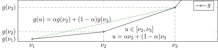
Figure 1: Convex lower envelope of a multibang regularizer and convex combinations $u=\alpha\nu_{2}+(1-\alpha)\nu_{3}$. For convex combinations between $g(\nu_{1})$ and $g(\nu_{3})$ (dotted green line), the evaluation of convex combinations and the evaluation of $g$ do not commute if $u$ is represented as a convex combination of $\nu_{1}$ and $\nu_{3}$.

Proposition 2.1.

Let $v^{n}\stackrel{{\scriptstyle\ast}}{{\rightharpoonup}}v$ in $L^{\infty}(\Omega)$ with $v(x)\in[\nu_{1},\nu_{M}]$ for a.a. $x\in\Omega$. For a.a. $x\in\Omega$ assume that $v(x)\in[\nu_{i},\nu_{i+1}]$ for some $i\in[M-1]$ implies $v^{n}(x)\in\{\nu_{i},\nu_{i+1}\}$ for all $n\in\mathbb{N}$. Then, $R(v^{n})\to R(v)$.

Proof.

The claim follows directly from the considerations above. ∎

Therefore, the function $R$ allows the identity (1.1) to be preserved. However, this does not mean that $R$ is a weakly-^∗-sequentially continuous function.

$R$ may be interpreted as a generalization of the $L^{1}$-regularization to promote $V$-valued controls with more than three bangs [10, Sect. 3]. The function $g$ above is the convex lower envelope of the function

$$g_{0}(u)\coloneqq\frac{\gamma}{2}|u|^{2}+\beta\prod_{i=1}^{M}|u-\nu_{i}|^{0}+\delta_{[\nu_{1},\nu_{M}]},$$ (2.4)

where $\delta_{[\nu_{1},\nu_{M}]}$ is the $\{0,\infty\}$-valued indicator function of the set $[\nu_{1},\nu_{M}]$, and $|0|^{0}=0$ and $|u|^{0}=1$ for $u\neq 0$ if the ratio $\beta/\gamma$ is large enough; see [9, Sect. 2] and [10, Sect. 3]. Because we do not use this particular structure, the following statement follows.

Corollary 2.2.

Let $g:[\nu_{1},\nu_{M}]\to\mathbb{R}$ be a positive, piecewise affine and convex function with the kinks connecting the affine pieces at $\{\nu_{1},\ldots,\nu_{M}\}$. Let $R(v)\coloneqq\int_{\Omega}g(v(x))\mathop{}\!\mathrm{d}x$. Let $v^{n}\stackrel{{\scriptstyle\ast}}{{\rightharpoonup}}v$ in $L^{\infty}(\Omega)$ with $v(x)\in[\nu_{1},\nu_{M}]$ for a.a. $x\in\Omega$. For a.a. $x\in\Omega$ assume that $v(x)\in[\nu_{i},\nu_{i+1}]$ for some $i\in\{1,\ldots,M-1\}$ implies $v^{n}(x)\in\{\nu_{i},\nu_{i+1}\}$ for all $n\in\mathbb{N}$. Then, $R(v^{n})\to R(v)$.

Proof.

Since $g:[\nu_{1},\nu_{M}]\to\mathbb{R}$ is a piecewise affine and convex function, its Clarke subdifferential $\partial^{c}g$ is

$$\partial^{c}g(u)=\left\{\begin{aligned} \{L_{i}\}&\text{ if }u\in(\nu_{i},\nu_{i+1})\text{ for some }i\in[M-1],\\ [-\infty,L_{i}]&\text{ if }u=\nu_{1},\\ [L_{i},L_{i+1}]&\text{ if }u=\nu_{i}\text{ for some }i\in[M-1],\\ [L_{M},\infty]&\text{ if }u=\nu_{M}\\ \end{aligned}\right.$$

for some $-\infty<L_{1}\leq\ldots\leq L_{M}<\infty$. Thus, $g$ has a constant slope of $L_{i}$ on $(\nu_{i},\nu_{i+1})$ for $i\in[M-1]$. Combining this with the prerequisite that $v(x)\in[\nu_{i},\nu_{i+1}]$ for some $i\in[M-1]$ implies $v^{n}(x)\in\{\nu_{i},\nu_{i+1}\}$ for all $n\in\mathbb{N}$, we again obtain that the evaluation of $g$ and the evaluation of the convex combination commute. The rest of the proof follows with the arguments above. ∎

Remark 2.3.

The assumption that for a.a. $x\in\Omega$ the inclusion $v(x)\in[\nu_{i},\nu_{i+1}]$ implies $v^{n}(x)\in\{\nu_{i},\nu_{i+1}\}$ for all $n\in\mathbb{N}$ constrains the algorithms that compute the $V$-valued controls $v^{n}$ for a given $v$ in the second step of the combinatorial integral approximation. Therefore, instead of computing the $V$-valued controls $v^{n}$ directly, binary-valued approximations $\omega^{n}$ of the coefficient function $\alpha$ are computed. Hence, the convergence $R(v^{n})\to R(v)$ hinges on satisfying (2.2) here. This insight enters our analysis in the general definition of $g$ in Definition 2.4 and the proof of Lemma 2.11.

2.2 Vector-Valued Controls

In [11], the multibang regularizer for vector-valued admissible controls is introduced as the choice $g\coloneqq\alpha c+\delta_{V}$, where $c$ is a positive strictly convex lower semicontinuous function and $\delta_{V}$ denotes the $\{0,\infty\}$-valued indicator function of the set $V$. Relaxations of multibang regularizers are then defined as the convex lower envelopes of such functions.

We take a different approach and define the considered class of regularizers for multidimensional controls geometrically. While this also yields polyhedral functions, it directly fits the algorithmic framework of the combinatorial integral approximation.

We recall that a function $f:\mathbb{R}^{m}\to\mathbb{R}\cup\{\infty\}$ is called polyhedral if its epigraph

$$\operatorname*{epi}f=\left\{(u,r)\in\mathbb{R}^{m}\times\mathbb{R}\,|\,f(u)\leq r\right\}$$

is a convex polyhedron. Next, we introduce the general class of regularizers, on which we focus in the remainder of the article.

Definition 2.4.

Let $V\subset\mathbb{R}^{m}$, and let $\{g_{1},\ldots,g_{M}\}\subset[0,\infty)$ satisfy the identity $\operatorname*{ext}\left(\operatorname*{conv}\{(\nu_{i},g_{i})\,|\,i\in[M]\}+\{(0,r)\,|\,r\geq 0\}\right)=\{(\nu_{i},g_{i})\,|\,i\in[M]\}$. Let $g:\mathbb{R}^{m}\to[0,\infty]$ be defined through

$$g(u)\coloneqq\left\{\begin{aligned} \infty&\text{ if }u\notin\operatorname*{conv}V,\\ \min\left\{\sum_{i=1}^{M}\alpha_{i}g_{i}\,\Bigg{|}\,\sum_{i=1}^{M}\alpha_{i}\nu_{i}=u,\sum_{i=1}^{M}\alpha_{i}=1,\alpha\geq 0\right\}&\text{ if }u\in\operatorname*{conv}V.\end{aligned}\right.$$

Then, we call the function $R(v)\coloneqq\int_{\Omega}g(v(x))\mathop{}\!\mathrm{d}x$ a relaxed multibang regularizer.

The positive scalars $g_{i}$ may be interpreted as a means to encode a preference of the different discrete control values $\nu_{i}$. We establish well-definedness and basic properties of relaxed multibang regularizers in the proposition below.

Proposition 2.5.

1. Let $g$ be as in Definition 2.4. Then, $g$ is well defined and polyhedral.

2. Let $g$ be as in Definition 2.4. Then, $g$ is Lipschitz continuous.

3. Let $g:\mathbb{R}^{m}\to[0,\infty]$ be polyhedral with nonempty bounded domain. Then, there exist $\{\nu_{1},\ldots,\nu_{M}\}\subset\mathbb{R}^{m}$ and $\{g_{1},\ldots,g_{M}\}\subset[0,\infty)$ such that $g$ can be stated in the form of Definition 2.4.

4. The function $R$ in Corollary 2.2 is a relaxed multibang regularizer.

Proof.

1. $u\in\operatorname*{conv}V$ can be represented as a convex combination of the $\nu_{i}$. Thus the feasible set of the LP defining $g(u)$ is nonempty. Moreover, the feasible set is a polytope and the LP admits a minimizer. Consequently, $g(u)$ is well defined.

To show that $g$ is polyhedral, we prove that $\operatorname*{epi}g=\operatorname*{conv}\{(\nu_{i},g_{i})\,|\,i\in[M]\}+\{(0,r)\,|\,r\geq 0\}$. The inclusion $\subset$ holds because $(u,g(u))\in\operatorname*{conv}\{(\nu_{i},g_{i})\,|\,i\in[M]\}$ for $g(u)<\infty$. To assert the inclusion $\supset$, we consider $(u,s)\in\operatorname*{conv}\{(\nu_{i},g_{i})\,|\,i\in[M]\}$ and $r\geq 0$. Then $(u,s)$ can be represented as a convex combination of the $(\nu_{i},g_{i})$, and the definition of $g(u)$ gives $g(u)\leq s\leq s+r$. Thus $(u,s)+(0,r)\in\operatorname*{epi}g$.

2. This follows from the Lipschitz continuity of LPs with respect to changes in the right-hand side in monotonic norms; see [26].

3. We use the inner description of the convex polyhedron $\operatorname*{epi}g$ and write $\operatorname*{epi}g=P+C$, where $P$ is a polytope and $C$ a finitely generated convex cone. Because the domain of $g$ is bounded and $g\geq 0$, it follows that we may choose $C=\{(0,r)\,|\,r\geq 0\}$ and that $\operatorname*{epi}g$ is pointed. Thus, $\operatorname*{epi}g$ has uniquely determined extremal points such that $P=\operatorname*{conv}\operatorname*{ext}\operatorname*{epi}g$. Consequently, the claim follows by setting $M\coloneqq|\operatorname*{ext}\operatorname*{epi}g|$ and defining the $(\nu_{i},g_{i})$ as the extremal points of $\operatorname*{epi}g$.

4. Because the function $g$ in Corollary 2.2 is piecewise affine and convex, it is polyhedral with domain $[\nu_{1},\nu_{M}]$, which proves the claim. ∎

Remark 2.6.

The assertions of Proposition 2.5 still hold if the relaxed identity $\operatorname*{ext}\operatorname*{conv}\{(\nu_{i},g_{i})\,|\,i\in[M]\}=\{(\nu_{i},g_{i})\,|\,i\in[M]\}$ is used or is relaxed further to $\operatorname*{int}\operatorname*{conv}\{(\nu_{i},g_{i})\,|\,i\in[M]\}\cap\{(\nu_{i},g_{i})\,|\,i\in[M]\}=\emptyset$.

Remark 2.7.

For $u\in\operatorname*{conv}V$, we consider minimizers $\alpha(u)$ of $g(u)$, that is

$$\alpha(u)\in\operatorname*{arg\,min}\left\{\sum_{i=1}^{M}\alpha_{i}g_{i}\,\Big{|}\,u=\sum_{i=1}^{M}\alpha_{i}\nu_{i},\sum_{i=1}^{M}\alpha_{i}=1,\alpha\geq 0\right\}.$$

The minimizers are unique in the setting of Corollary 2.2, but this is not always true. For example, consider $V=\left\{(1\enskip 0)^{T},(0\enskip 1)^{T},(-1\enskip 0)^{T},(0\enskip-1)^{T}\right\}$ and $g_{i}=1$ for $i\in\{1,\ldots,4\}$. Then, several convex combinations exist for $u=(0\enskip 0)^{T}$, and $\sum_{i=1}^{4}\alpha_{i}g_{i}=1$ holds for all of them.

2.3 Selection Functions for Convex Coefficients

The algorithms for the second step of the combinatorial integral approximation operate on functions of convex coefficients $\alpha:\Omega\to[0,1]^{M}$ with $v(x)=\sum_{i=1}^{M}\alpha_{i}(x)\nu_{i}$ a.e. instead of the function $v$ directly. Thus, for a given control $v:\Omega\to\operatorname*{conv}V$, we need to recover convex coefficients $\alpha(x)\in\mathbb{R}^{M}$ for a.a. $x\in\Omega$ that minimize the LPs defining $g(v(x))$.

We desire a measurable function $\alpha:\Omega\to[0,1]^{M}$. Because the LPs defining $g(v(x))$ for $x\in\Omega$ do not necessarily have unique minimizers and a selection function $\alpha(x)$ is not readily available in closed form, the existence and computation of a measurable selection function $\alpha$ are not immediate. We consider the set-valued optimal policy function $G:\operatorname*{conv}V\rightrightarrows\mathbb{R}^{M}$, which is defined as

$$G(u)\coloneqq\operatorname*{arg\,min}\left\{\sum_{i=1}^{M}\alpha_{i}g_{i}\,\Bigg{|}\,u=\sum_{i=1}^{M}\alpha_{i}\nu_{i},\sum_{i=1}^{M}\alpha_{i}=1,\alpha\geq 0\right\}$$ (2.5)

for all $u\in\operatorname*{conv}V$. Thus, we require a measurable selector function $\tilde{g}:\operatorname*{conv}V\to\mathbb{R}^{M}$ for $G$. We recall that the multifunction $G$ is weakly measurable if the set $\{u\in\operatorname*{conv}V\,|\,G(u)\cap U\neq\emptyset\}$ is Borel measurable for all open sets $U\subset\mathbb{R}^{M}$. The following abstract result follows from the literature.

Lemma 2.8.

The multifunction $G$ is weakly measurable and admits a measurable selector $\phi:\operatorname*{conv}V\to\mathbb{R}^{M}$.

Proof.

We combine the Kuratowski–Ryll–Nardzewski measurable selection theorem [23] with the fact that the set $G(u)$ depends continuously on the vector $u$ [4]. ∎

The measurability of the multifunction $G$ allows us to prove measurability for a large class of possible selector functions.

Lemma 2.9.

Let $\eta:\mathbb{R}^{M}\to\mathbb{R}$ be strictly convex and lower semi-continuous. Then, the function $\tilde{g}(u)\coloneqq\operatorname*{arg\,min}\left\{\eta(\alpha)\,|\,\alpha\in G(u)\right\}$ is single-valued and measurable. In particular, $\tilde{g}$ defined as $\tilde{g}(u)\coloneqq\operatorname*{arg\,min}\{\|\alpha\|_{2}^{2}\,|\,\alpha\in G(u)\}$ for $u\in\operatorname*{conv}V$ is measurable.

Proof.

We observe that $G$ is weakly measurable (Lemma 2.8) and compact-valued. Then, we apply [18, Thm. 2 & 3] with the choices $u\coloneqq-\eta$ and $f\coloneqq\tilde{g}$. The optimization problem $\min\{\eta(\alpha)\,|\,\alpha\in G(u)\}$ has a unique solution for $u\in\operatorname*{conv}V$. The existence of a minimizer follows from compactness of $G(u)$ and lower semi-continuity of $\eta$. The uniqueness follows from the strict convexity of $\eta$. Therefore, the selector $\tilde{g}$ is single-valued and can be interpreted as a function $\tilde{g}:\operatorname*{conv}V\to\mathbb{R}^{M}$. ∎

2.4 Proof of the Identity (1.1)

We prove the identity (1.1) for relaxed multibang regularizers by showing that for a $\operatorname*{conv}V$-valued control $v$, there exist $V$-valued controls $v^{n}$ such that $R(v)=\liminf R(v^{n})$ holds. Before this result is proven in Lemma 2.11, we show an auxiliary lemma.

Lemma 2.10.

Let $R(v)\coloneqq\int_{\Omega}g(v(x))\,\mathop{}\!\mathrm{d}x$ be a relaxed multibang regularizer. Then, the function $g$ defined in Definition 2.4 and $G$ defined in (2.5) satisfy $g(\nu_{i})=g_{i}$ and $G(\nu_{i})=\{e_{i}\}$ for $i\in[M]$, where $e_{i}$ is the $i$th canonical unit vector in $\mathbb{R}^{M}$.

Proof.

Let $i\in[M]$. The vector $e_{i}$ is feasible for the LP defining $g(\nu_{i})$ with objective value $g_{i}$, which gives $g(\nu_{i})\leq g_{i}$. Let $\alpha\in G(\nu_{i})$ and $\alpha\neq e_{i}$. We proceed by contradiction and distinguish the cases $g(\nu_{i})=g_{i}$ and $g(\nu_{i})<g_{i}$.

Let $\sum_{i=1}^{M}\alpha_{i}\nu_{i}=\nu_{i}$ and $\sum_{i=1}^{M}\alpha_{i}g_{i}=g_{i}$. Then,

$$(\nu_{i},g_{i})\notin\operatorname*{ext}\left(\operatorname*{conv}\{(\nu_{i},g_{i})\,|\,i\in[M]\}+\{(0,r)\,|\,r\geq 0\}\right),$$

a contradiction to Definition 2.4. Let $\sum_{j=1}^{M}\alpha_{j}\nu_{j}=\nu_{i}$ and $\sum_{j=1}^{M}\alpha_{j}g_{j}<g_{i}$. Then, we can write $g_{i}=\eta\left(\sum_{j=1}^{M}\alpha_{j}g_{j}\right)+(1-\eta)2g_{i}$ for some $\eta\in(0,1)$. Clearly $\eta\sum_{j=1}^{M}\alpha_{j}\nu_{j}+(1-\eta)\nu_{i}=\nu_{i}$. Again, we obtain

$$(\nu_{i},g_{i})\notin\operatorname*{ext}\left(\operatorname*{conv}\{(\nu_{i},g_{i})\,|\,i\in[M]\}+\{(0,r)\,|\,r\geq 0\}\right),$$

which contradicts Definition 2.4. Thus, $e_{i}$ is the only feasible point for the LP that defines $g(\nu_{i})$, and we deduce $g(\nu_{i})=g_{i}$ and $G(\nu_{i})=\{e_{i}\}$. ∎

Lemma 2.11.

Let $R$ be a relaxed multibang regularizer. Let $v\in L^{\infty}(\Omega,\mathbb{R}^{m})$ with $R(v)<\infty$. Then, there exists a sequence of functions $(v^{n})_{n}\subset L^{\infty}(\Omega,\mathbb{R}^{m})$ that are $V$-valued such that $v^{n}\stackrel{{\scriptstyle\ast}}{{\rightharpoonup}}v$ in $L^{\infty}(\Omega,\mathbb{R}^{m})$ and $R(v)=\lim_{n\to\infty}R(v^{n})$.

Proof.

Because $R(v)<\infty$, we can assume that $v(x)\in\operatorname*{conv}V$ a.e. Lemma 2.8 gives the existence of a measurable selector function $\phi$ for the LP solution sets that defines the values of the integrand $g$ of $R$. Because $v$ is measurable and $\operatorname*{conv}V$-valued a.e., the function $\alpha:\Omega\to\mathbb{R}^{M}$ defined as $\alpha(x)\coloneqq\phi(v(x))$ a.e. is in $L^{\infty}(\Omega,\mathbb{R}^{M})$.

Definition 3.1 implies $\alpha(x)\geq 0$, $\sum_{i=1}^{M}\alpha_{i}(x)=1$, and $v(x)=\sum_{i=1}^{M}\alpha_{i}(x)\nu_{i}$. We can apply the multidimensional sum-up rounding algorithm on a sequence of suitably refined grids (see [29]) to obtain a sequence of $\{0,1\}^{M}$-valued functions $\omega^{n}$ such that $\sum_{i=1}^{M}\omega_{i}^{n}(x)=1$ holds a.e. and for all $n$. Then, $\omega^{n}\stackrel{{\scriptstyle\ast}}{{\rightharpoonup}}\alpha$ follows from the analysis in [29]. We define $v^{n}(x)\coloneqq\sum_{i=1}^{M}\omega^{n}_{i}(x)\nu_{i}$ a.e. and for all $n$, and we deduce

$$R(v) =\int_{\Omega}g(v(x))\,\mathop{}\!\mathrm{d}x=\int_{\Omega}\sum_{i=1}^{M}g_{i}\alpha_{i}(x)\,\mathop{}\!\mathrm{d}x$$

$$=\sum_{i=1}^{M}g_{i}\int_{\Omega}\alpha_{i}(x)\,\mathop{}\!\mathrm{d}x=\lim_{n\to\infty}\sum_{i=1}^{M}g_{i}\int_{\Omega}\omega^{n}_{i}(x)\,\mathop{}\!\mathrm{d}x=\lim_{n\to\infty}\int_{\Omega}\sum_{i=1}^{M}g_{i}\omega^{n}_{i}(x)\,\mathop{}\!\mathrm{d}x.$$

Thus, it remains to show that

$$\int_{\Omega}\sum_{i=1}^{M}g_{i}\omega^{n}_{i}(x)\,\mathop{}\!\mathrm{d}x=\int_{\Omega}g\left(\sum_{i=1}^{M}\nu_{i}\omega^{n}_{i}(x)\right)\,\mathop{}\!\mathrm{d}x=R(v^{n}).$$ (2.6)

For a.a. $x\in\Omega$, there exists $i\in[M]$ such that $\omega^{n}_{i}(x)=1$ and $\omega^{n}_{j}(x)=0$ for $j\neq i$. This implies

$$g(v^{n}(x))=g(\omega^{n}_{i}(x)\nu_{i})=g(\nu_{i})\underset{\textrm{Lem.\ \ref{lem:rel_mbreg_extremaloptimality}}}{=}g_{i}=\sum_{i=1}^{M}g_{i}\omega^{n}_{i}(x).$$ (2.7)

Integrating (2.7) over $\Omega$ yields (2.6), which closes the argument. ∎

Having obtained Lemma 2.11, we are prepared to prove the identity (1.1).

Theorem 2.12.

Let $\Omega$ be a bounded domain. Let $F:L^{\infty}(\Omega,\mathbb{R}^{m})\to\mathbb{R}$ be weakly-^∗-sequentially continuous. Let $V=\{\nu_{1},\ldots,\nu_{M}\}\subset\mathbb{R}^{m}$ and $\{g_{1},\ldots,g_{M}\}\subset[0,\infty)$ satisfy the assumptions of Definition 2.4, and let $R$ be defined as in Definition 2.4. Then, (R) admits a minimizer, and the identity (1.1) holds.

Proof.

Because $\mathbb{R}^{m}$ is a Euclidean space, the space $L^{\infty}(\Omega,\mathbb{R}^{m})$ admits a weak-^∗-topology. From the Lyapunov convexity theorem—consider, for example, the version [41, Thm. 3]—we have that the feasible set $\mathcal{F}_{\eqref{eq:r}}$ of (R) is weakly-^∗-compact.

The weak-^∗-sequential continuity of $F$ gives that $F$ is bounded on $\mathcal{F}_{\eqref{eq:r}}$. For $g$ defined in Definition 2.4, $\operatorname*{epi}g$ is a convex polyhedron and therefore closed. Thus, $g$ is a convex proper continuous function with bounded domain. Consequently, $R:L^{\infty}(\Omega,\mathbb{R}^{m})\to[0,\infty]$ is a weakly-^∗-sequentially lower semicontinuous function (see, e.g., [13, Thm. 5.14]) and bounded from below. The existence of a minimizer for (R) follows with the direct method of calculus of variations.

Let $v$ be a minimizer of (R). Lemma 2.11 gives that there exists a sequence of functions $(v^{n})_{n}$ that are feasible for (P) such that $R(v)=\lim R(v^{n})$. The sequence $(v^{n})_{n}$ provided by Lemma 2.11 satisfies $v^{n}\stackrel{{\scriptstyle\ast}}{{\rightharpoonup}}v$. The claim follows from the weak-^∗-sequential continuity of $F$ and $R(v)=\lim R(v^{n})$. ∎

Remark 2.13.

The identity $\int_{\Omega}g(v(x))\,\mathop{}\!\mathrm{d}x=\int_{\Omega}\sum_{i=1}^{M}g_{i}\alpha_{i}(x)\,\mathop{}\!\mathrm{d}x$ in Lemma 2.11 is the key step to prove the identity (1.1). The assumptions on the pairs $(\nu_{i},g_{i})$ and the pointwise definition of $g$ as the minimum of an LP allow that evaluating convex combinations of the $\nu_{i}$ and evaluating $g$ commute. Suboptimal convex combinations would result in a gap between $R(v)$ and $\liminf R(v^{n})$; see again Figure 1.

2.5 Smoothing of $R$

We recall that the Moreau envelope of a proper lower semicontinuous function $f:\mathbb{R}^{m}\to\mathbb{R}\cup\{\infty\}$ is defined as

$$(e_{\gamma}f)(x)\coloneqq\inf\left\{f(y)+\frac{1}{2\gamma}\|x-y\|^{2}_{2}\,\Big{|}\,y\in\mathbb{R}^{m}\right\}$$

for $\gamma>0$. Let $R$ given as $R(v)=\int_{\Omega}g(v(x))\,\mathop{}\!\mathrm{d}x$ be a relaxed multibang regularizer. Then for $\gamma>0$, we define the function

$$R_{\gamma}(v)\coloneqq\int_{\Omega}(e_{\gamma}g)(v(x))\,\mathop{}\!\mathrm{d}x.$$

Moreover, we define the following smoothed control problems, (R_γ) for $\gamma>0$,

$$\begin{aligned} \min_{v}\ &\mathcal{F}(v)+R_{\gamma}(v)\\ \text{ s.t.\ }&v\in L^{\infty}(\Omega,\mathbb{R}^{m})\text{ and }v(x)\in\operatorname*{conv}\{\nu_{1},\ldots,\nu_{M}\}\text{ for a.a.\ }x\in\Omega,\end{aligned}$$ (R_γ)

and set (R₀) $\coloneqq$ (R). We summarize the convexity and differentiability properties and the convergence of minimizers of the (R_γ) to minimizers of (R) for $\gamma\downarrow 0$ below. As for (P) we denote the infimal value of the (R_γ) by $\inf\eqref{eq:rgamma}$.

The basic properties of the Moreau envelope yield the following properties.

Proposition 2.14.

1. Let $u\in\operatorname*{conv}V$. Then, $(e_{\gamma}g)(u)\uparrow g(u)$ for $\gamma\downarrow 0$.

2. Let $v\in\mathcal{F}_{\eqref{eq:r}}$. Then, $R_{\gamma}(v)\uparrow R(v)$ for $\gamma\downarrow 0$.

3. Let $\gamma>0$. Then, the function $e_{\gamma}g:\operatorname*{conv}V\to\mathbb{R}$ is convex and continuously differentiable with the Lipschitz-continuous derivative.

4. Let $\gamma>0$, and $p\geq 2$. Then, $R_{\gamma}:L^{p}(\Omega,\mathbb{R}^{m})\to\mathbb{R}$ is differentiable with derivative $R_{\gamma}^{\prime}(v)d=\int_{\Omega}(e_{\gamma}g)^{\prime}(v(x))^{T}d(x)\,\mathop{}\!\mathrm{d}x$ for $d\in L^{p}(\Omega,\mathbb{R}^{m})$.

Proof.

Basic properties of the Moreau envelope [31, Sect. 1.G] yield Claim 1. Claim 2 follows from Beppo–Levi’s theorem with Claim 1. Claim 3 follows from [31, Thm. 2.26] and the firm nonexpansiveness of the proximal mapping. The chain rule and differentiability properties of Nemitskij operators [15, Thm. 7] yield Claim 4. ∎

Proposition 2.15.

Let $(\gamma^{n})_{n}\subset[0,\infty)$ satisfy $\gamma^{n}\downarrow 0$. Then, the sequence of functionals $F+R_{\gamma^{n}}$ on $\mathcal{F}_{\eqref{eq:r}}\subset L^{\infty}(\Omega,\mathbb{R}^{m})$ is $\Gamma$-convergent with limit $F+R$ with respect to weak-^∗-convergence in $L^{\infty}$.

Proof.

Because $F$ is weak-^∗-sequentially continuous, it suffices to prove that $R$ is a $\Gamma$-limit for the sequence $(R_{\gamma^{n}})_{n}$. Let $L>0$ denote the Lipschitz constant of $g$, which exists by virtue of Proposition 2.5 2. Then, we obtain

$$R(w)-R_{\gamma^{n}}(w)=\int_{\Omega}g(w(x))-(e_{\gamma^{n}}g)(w(x))\,\mathop{}\!\mathrm{d}x\leq\frac{1}{2}\lambda(\Omega)L^{2}\gamma^{n}$$ (2.8)

for all $w\in\mathcal{F}_{\eqref{eq:r}}$, where $\lambda(\Omega)$ denotes the Lebesgue measure of $\Omega$. We defer the proof to Section A.2. Let $v^{n}$, $v\in\mathcal{F}_{\eqref{eq:r}}$ for all $n\in\mathbb{N}$ be such that $v^{n}\stackrel{{\scriptstyle\ast}}{{\rightharpoonup}}v$ in $L^{\infty}(\Omega,\mathbb{R}^{m})$. Because $R$ is weak-^∗-sequentially lower semicontinuous, it follows that

$$R(v)\leq\liminf R(v^{n})\leq\liminf R_{\gamma^{n}}(v^{n})+\frac{1}{2}\lambda(\Omega)L^{2}\gamma^{n}=\liminf R_{\gamma^{n}}(v^{n}),$$

where the second inequality follows from (2.8) with the choice $w=v^{n}$.

By virtue of Proposition 2.14 it follows that $R_{\gamma^{1}}(v)\leq R_{\gamma^{n}}(v)\leq R_{\gamma^{n+1}}(v)\leq R(v)$ holds for all $n\in\mathbb{N}$. Combining these estimates, we obtain $\Gamma$-convergence. ∎

Corollary 2.16.

Let $(\gamma^{n})_{n}\subset[0,\infty)$ satisfy $\gamma^{n}\downarrow 0$, and let $(\varepsilon^{n})_{n}\subset[0,\infty)$ satisfy $\varepsilon^{n}\to 0$. Let $v$, $v^{n}\in\mathcal{F}_{\eqref{eq:r}}$ for $n\in\mathbb{N}$ satisfy $v^{n}\stackrel{{\scriptstyle\ast}}{{\rightharpoonup}}v$ and $F(v^{n})+R_{\gamma_{n}}(v^{n})<\varepsilon^{n}+\inf\text{\emph{(R${}_{\gamma^{n}}$)}}$. Then, $v$ is a minimizer of (R).

Proof.

This follows with a standard proof from $\Gamma$-convergence; see, e.g., [12]. ∎

Remark 2.17.

This approach differs from the Moreau–Yosida regularization performed in [11]. Therein, the authors work with a Moreau envelope of the convex conjugate of the relaxed multibang regularizer $R$, specifically $(e_{\gamma}R^{*})^{*}(v)=R(v)+\frac{\gamma}{2}\|v\|^{2}$. They improve the convergence of the sequence of minimizing controls for (R) to norm-convergence. This is enabled by the strict convexity that is added by the term $\frac{\gamma}{2}\|v\|^{2}$. The resulting regularized multibang regularizer is nondifferentiable, and nonsmooth techniques are necessary for the optimization; see also [11, Rem. 2.3].

3 Algorithmic Framework

We use the properties of relaxed multibang regularizers and the optimization problems (R) and (R_γ) to formulate an algorithm to compute minimizing control sequences for (P). In Section 3.1 we provide the necessary concepts to formulate the second step of the combinatorial integral approximation, specifically so-called rounding algorithms. In Section 3.2 we integrate these concepts with the findings from Section 2 into one algorithm, for which we prove well-definedness and asymptotics. Practical aspects for the solution of the involved optimization problems are considered in Section 3.3.

3.1 Rounding Algorithms

We introduce the concepts of rounding grid and of order-conserving dissection [29] before defining rounding algorithms. A rounding grid is a partition of the domain $\Omega$. An order-conserving domain dissection is a sequence of refined rounding grids that satisfies certain regularity properties.

Definition 3.1.

Let $\Omega\subset\mathbb{R}^{d}$ be a bounded domain. We call a finite partition $\mathcal{T}=\left\{T_{1},\ldots,T_{N}\right\}\in 2^{\Omega}$ of $\Omega$ into $N\in\mathbb{N}$ grid cells a rounding grid. We denote its maximum grid cell volume by $\Delta_{\mathcal{T}}=\max\{\lambda(T_{i})\,|\,i\in[N]\}$.

We call a sequence of rounding grids $(\mathcal{T}^{n})_{n}\subset 2^{\mathcal{B}(\Omega)}$ with $\mathcal{T}^{n}=\left\{T_{1}^{n},\ldots,T_{N^{n}}^{n}\right\}$ and corresponding maximum grid cell volumes for all $n\in\mathbb{N}$ an order-conserving domain dissection of $\Omega$ if

1. $\Delta_{\mathcal{T}^{n}}\to 0$,

2. for all $n$ and all $i\in[N^{n-1}]$, there exist $1\leq j<k\leq N^{n}$ such that $\bigcup_{l=j}^{k}T_{l}^{n}=T_{i}^{n-1}$, and

3. the cells $T^{n}_{j}$ shrink regularly; that is, there exists $C>0$ such that for each $T_{j}^{n}$ there exists a Ball $B_{j}^{n}$ such that $T_{j}^{n}\subset B_{j}^{n}$ and $\lambda(T_{j}^{n})\geq C\lambda(B_{j}^{n})$.

Definition 3.1 1 requires that the maximum volume of the grid cells of a rounding grid vanish over the refinements. Definition 3.1 2 requires that a grid cell of a rounding grid be decomposed into finitely many grid cells in the next rounding grid and that the order of the grid cells of a partition be conserved by the grid cells in which it is decomposed in all later iterations. Definition 3.1 3 requires that the grid cells shrink regularly. In particular, their eccentricity remains bounded over the iterations.

Example 3.2.

Definition 3.1 is, for example, satisfied by uniform refinements of a uniform mesh, where the order of the grid cells is induced by the course of approximants of space-filling curves through the grid cells [29].

We introduce the terms binary and relaxed control [29] to denote output and input functions of the rounding algorithms. Then, we introduce pseudometrics induced by rounding grids to describe the approximation relationship between input and output of rounding algorithms.

Definition 3.3.

Let $\Omega\subset\mathbb{R}^{d}$ be a bounded domain. We call measurable functions $\omega:\Omega\to\{0,1\}^{M}$ such that $\sum_{i=1}^{M}\omega_{i}(x)=1$ holds a.e. binary controls. We call measurable functions $\alpha:\Omega\to[0,1]^{M}$ such that $\sum_{i=1}^{M}\alpha_{i}(x)=1$ holds a.e. relaxed controls.

Definition 3.4.

Let $\mathcal{T}$ be a rounding grid. We define its induced pseudometric for relaxed controls $\alpha$ and $\beta$ as

$$d_{\mathcal{T}}(\alpha,\beta)\coloneqq\max\left\{\left\|\int_{\bigcup_{i=1}^{k}T_{i}}\alpha(x)-\beta(x)\,\mathop{}\!\mathrm{d}x\right\|_{\infty}\,\Bigg{|}\,k\in[N]\right\}.$$

It is straightforward that $d_{\mathcal{T}}(\alpha,\beta)$ is a pseudometric on $L^{\infty}(\Omega,\mathbb{R}^{M})$. Convergence with respect to the sequence of $(d_{\mathcal{T}^{n}})_{n}$ induced by an order conserving domain dissection implies weak-^∗-convergence in $L^{\infty}$ [22]. Because $d_{\mathcal{T}}$ cannot distinguish relaxed controls that have the same average value per grid cell, we will approximate an solution of (R_γ) that is averaged per grid cell. Thus, for a function $v:\Omega\to\operatorname*{conv}V$ and a rounding grid $\mathcal{T}$, we define its average per grid cell $\bar{v}:\Omega\to\operatorname*{conv}V$ as

$$\bar{v}\coloneqq\sum_{i=1}^{N}\chi_{T_{i}}\frac{1}{\lambda(T_{i})}\int_{T_{i}}v(x)\,\mathop{}\!\mathrm{d}x.$$ (3.1)

We use rounding algorithms as functions that map relaxed controls to binary controls and provide an approximation in $d_{\mathcal{T}}$, which yields the definition below.

Definition 3.5.

A rounding algorithm is a function $\operatorname*{\mathcal{RA}}$ that maps a rounding grid $\mathcal{T}$ and a relaxed control $\alpha$ to a binary control $\omega$; that is, $\omega=\operatorname*{\mathcal{RA}}(\mathcal{T},\alpha)$. In particular, there exists a constant $\theta>0$ such that $d_{\mathcal{T}}(\alpha,\omega)\leq\theta\Delta_{\mathcal{T}}$ holds for all relaxed controls $\alpha$, all rounding grids $\mathcal{T}$, and $\omega=\operatorname*{\mathcal{RA}}(\mathcal{T},\alpha)$.

Remark 3.6.

Definition 3.5 is satisfied for sum-up rounding (SUR) [35], next-forced rounding (NFR) [19], and the optimization-based approaches presented in [19, 3], which have all been used in the combinatorial integral approximation framework.

3.2 Main Algorithm

We introduce the algorithmic framework as Algorithm 1. Before proving the asymptotics of Algorithm 1 we argue below that its steps are well defined. The critical steps that require consideration are the finite termination of the for loop beginning in Line 4 and the computation of $\alpha^{n}$ in Line 11.

Algorithm 1 Approximation of (P)

Input: Order-conserving sequence of rounding grids $(\mathcal{T}^{n})_{n}$.

Input: Rounding algorithm $\operatorname*{\mathcal{RA}}$.

Input: Null sequences $\varepsilon^{n}\downarrow 0$ and $\gamma^{n}\downarrow 0$.

1:$c^{0}\leftarrow 0$

2:for $n=0,\ldots$ do

3:      Compute $v^{n}$ such that $F(v^{n})+R_{\gamma^{n}}(v^{n})<\varepsilon^{n}+\inf\text{(R${}_{\gamma^{n}}$)}$.

4:     for $k=1,\ldots$ do

5:         Compute avg. per grid cell $\bar{v}^{n}$ (see (3.1)) from $v^{n}$ on rounding grid $\mathcal{T}^{c^{n}}$.

6:         if $\|\bar{v}^{n}-v^{n}\|_{L^{2}(\Omega)}<\varepsilon^{n}$ then

7:              break

8:         end if

9:         $c^{n}\leftarrow c^{n}+1$

10:     end for

11:      Compute $\alpha^{n}(x)\coloneqq\operatorname*{arg\,min}\{\|a\|_{2}^{2}\,|\,a\in G(\bar{v}^{n}(x))\}$ with $G$ defined in (2.5).

12:      Compute binary control $\omega^{n}=\operatorname*{\mathcal{RA}}(\mathcal{T}^{c^{n}},\alpha^{n})$.

13:      Compute $\{\nu_{1},\ldots,\nu_{M}\}$-valued control $\hat{v}^{n}\coloneqq\sum_{i=1}^{M}\omega^{n}_{i}\nu_{i}$.

14:      $c^{n+1}\leftarrow c^{n}$.

15:end for

Proposition 3.7.

Let $R$ be a relaxed multibang regularizer. Let the inputs of Algorithm 1 be given. For all iterations $n\in\mathbb{N}$ of Algorithm 1 it holds that

1. the for loop starting in Line 4 terminates after finitely many iterations and

2. $\alpha^{n}$ is a uniquely defined relaxed control.

Proof.

1. Definition 3.1 3 implies that order-conserving domain dissections satisfy the prerequisites of the Lebesgue differentiation theorem [40, Chap. 3, Cor. 1.6 & 1.7]. Thus $\bar{v}^{n}\to v^{n}$ pointwise a.e. for $k\to\infty$. Because $v^{n}(x)\in\operatorname*{conv}\{\nu_{1},\ldots,\nu_{M}\}$ a.e., which translates to $\bar{v}^{n}$ computed in the $k$th iteration, Lebesgue’s dominated convergence theorem gives $\bar{v}^{n}\to v^{n}$ in $L^{2}(\Omega)$ for $k\to\infty$. Since $\varepsilon^{n}>0$ for all $n\in\mathbb{N}$, the termination criterion $\|\bar{v}^{n}-v^{n}\|_{L^{2}(\Omega)}<\varepsilon^{n}$ is satisfied after a finite number of iterations of the inner loop.

2. Lemma 2.9 gives that $\min\{\|a\|_{2}^{2}\,|\,a\in G(u)\}$ has a unique minimizer that satisfies $\sum_{i=1}^{M}a_{i}=1$ and $a\geq 0$ for all $u\in\operatorname*{conv}V$. Moreover, the function $\bar{v}^{n}$ is piecewise constant on the cells of a finite decomposition of $\Omega$. Third, we observe that $\alpha^{n}$ is measurable from the fact that $\bar{v}^{n}$ is measurable and from Lemma 2.9. ∎

Now, we state our main result, the convergence of the iterates produced by Algorithm 1. Then, we prove an auxiliary lemma before proving the theorem.

Theorem 3.8.

Let $R$ be a relaxed multibang regularizer. Let the inputs of Algorithm 1 be given. Then, Algorithm 1 produces an infinite sequence of iterates $v^{n}$, $\bar{v}^{n}$, $\hat{v}^{n}\in L^{\infty}(\Omega,\mathbb{R}^{m})$ such that $v^{n}$ admits a weak-^∗-cluster point and any weak-^∗-cluster point $v^{*}$ of $(v^{n})_{n}$ satisfies the following:

1. there is a subsequence $v^{n_{k}}\stackrel{{\scriptstyle\ast}}{{\rightharpoonup}}v^{*}$ that minimizes (R),

2. $\bar{v}^{n_{k}}\stackrel{{\scriptstyle\ast}}{{\rightharpoonup}}v^{*}$,

3. $\hat{v}^{n_{k}}\stackrel{{\scriptstyle\ast}}{{\rightharpoonup}}v^{*}$,

4. $F(\hat{v}^{n_{k}})\to F(v^{*})$,

5. $R(\hat{v}^{n_{k}})\to R(v^{*})$, and in particular

6. $(\hat{v}^{n_{k}})_{k}$ is a minimzing sequence for (P).

We prove that $R(\bar{v}^{n})$ and $R(\hat{v}^{n})$ are close for $n\to\infty$ as an independent lemma.

Lemma 3.9.

Let $R$ be a relaxed multibang regularizer. Let the inputs of Algorithm 1 be given. There exists $C>0$ such that for $\bar{v}^{n}$ and $\hat{v}^{n}$ computed by Algorithm 1 lines 4 to 13 from $v^{n}\in\mathcal{F}_{\eqref{eq:r}}$ it holds that $\left|R(\bar{v}^{n})-R(\hat{v}^{n})\right|\leq C\Delta_{\mathcal{T}^{c^{n}}}$. The constant $C>0$ does not depend on the rounding grids $\mathcal{T}^{c^{n}}$.

Proof.

Because we consider a fixed iteration $n$, we omit the index $n$ for the functions as well as the index $c^{n}$ for the rounding grid in this proof. From the construction of $\alpha$ in Line 11 we obtain $R(\bar{v})=\int_{\Omega}g(\bar{v}(x))\,\mathop{}\!\mathrm{d}x=\int_{\Omega}\sum_{i=1}^{M}\alpha_{i}(x)g_{i}\,\mathop{}\!\mathrm{d}x$. Because $\omega=\operatorname*{\mathcal{RA}}(\mathcal{T},\alpha)$, we have that $\omega$ is a binary control, which implies

$$R(\hat{v})=\int_{\Omega}g(\hat{v}(x))\,\mathop{}\!\mathrm{d}x=\int_{\Omega}\sum_{i=1}^{M}\omega_{i}(x)g(\nu_{i})\,\mathop{}\!\mathrm{d}x=\int_{\Omega}\sum_{i=1}^{M}\omega_{i}(x)g_{i}\,\mathop{}\!\mathrm{d}x,$$

where the last equality follows from Lemma 2.9. We conclude

$$\left|R(\bar{v})-R(\hat{v})\right|\leq\sum_{i=1}^{M}|g_{i}|\left|\int_{\Omega}\alpha_{i}(x)-\omega_{i}(x)\,\mathop{}\!\mathrm{d}x\right|\leq\sum_{i=1}^{M}|g_{i}|d_{\mathcal{T}}(\alpha,\omega),$$

where the first inequality follows from the triangle inequality and the second inequality by definition of $d_{\mathcal{T}}$. Because of Definition 3.5, the claim follows with the choice $C\coloneqq\sum_{i=1}^{M}|g_{i}|\theta$. ∎

We are ready to prove our main result.

Proof of Theorem 3.8.

For the statements of Theorem 3.8 to be well defined, we require that the inner loop (indexed by $k$) of Algorithm 1 terminates finitely for all $n\in\mathbb{N}$. This follows from Proposition 3.7. The existence of weak-^∗-cluster points follows from the boundedness of the sequence. We prove the claims one by one.

1. The minimization property of weakly-^∗-convergent subsequences follows directly from Corollary 2.16.

2. follows from the finite termination of the inner loop, in particular $\|\bar{v}^{n_{k}}-v^{n_{k}}\|_{L^{2}(\Omega)}\to 0$, and $v^{n_{k}}\stackrel{{\scriptstyle\ast}}{{\rightharpoonup}}v^{*}$.

3. We consider the construction of $\hat{v}^{n_{k}}$ and obtain

$$\hat{v}^{n_{k}}=\sum_{i=1}^{M}\omega^{n_{k}}_{i}\nu_{i}=\sum_{i=1}^{M}(\omega^{n_{k}}_{i}-\alpha^{n_{k}}_{i})\nu_{i}+\sum_{i=1}^{M}\alpha^{n_{k}}_{i}\nu_{i}=\sum_{i=1}^{M}(\omega^{n_{k}}_{i}-\alpha^{n_{k}}_{i})\nu_{i}+\bar{v}^{n_{k}}.$$

Then, we test with $f\in L^{1}(\Omega,\mathbb{R}^{m})$ and apply [29, Lem. 4.4] to obtain that the difference term vanishes weakly-^∗ for $k\to\infty$. We deduce

$$\lim_{k\to\infty}\langle v^{n_{k}},f\rangle_{L^{1},L^{\infty}}=\lim_{k\to\infty}\langle\bar{v}^{n_{k}},f\rangle_{L^{1},L^{\infty}}=\langle v^{*},f\rangle_{L^{1},L^{\infty}}.$$

4. follows from 3. and the weak-^∗-sequential continuity of $F$.

5. We estimate

$$\left|R(\hat{v}^{n_{k}})-R(v^{*})\right|\leq\left|R(\hat{v}^{n_{k}})-R(\bar{v}^{n_{k}})\right|+\left|R(\bar{v}^{n_{k}})-R(v^{n_{k}})\right|+\left|R(v^{n_{k}})-R(v^{*})\right|$$

by means of the triangle inequality. Because the rounding algorithm is executed on grids of an order-conserving domain dissection and $c^{n_{k}}\to\infty$, the first term tends to zero by virtue of Lemma 3.9. The finite termination of the inner loop and $\varepsilon^{n_{k}}\to 0$ imply that the second term tends to zero. It remains to show $\left|R(v^{n_{k}})-R(v^{*})\right|\to 0$. To this end, we estimate

$$\left|R(v^{n_{k}})-R(v^{*})\right| \leq\left|R_{\gamma_{n_{k}}}(v^{n_{k}})-R(v^{n_{k}})\right|+\left|R_{\gamma_{n_{k}}}(v^{n_{k}})-R(v^{*})\right|$$

by means of the triangle inequality. The first term tends to zero by virtue of (2.8). The second term tends to zero by combining 1. with 4. ∎

Remark 3.10.

Minimizers of (R) are generally fractional-valued. Thus, an approximation with discrete-valued controls can only achieve weak-^∗-convergence in $L^{p}$-spaces and norm-convergence is only conceivable for discrete-valued minimizers.

3.3 Practical Considerations

The fact that we require $v^{n}$ to be $\varepsilon^{n}$-optimal for (R) allows us to replace the infinite-dimensional optimization problem (R${}_{\gamma^{n}}$) by successively refined discretized finite-dimensional problems using, for example, the argument in [17].

In Algorithm 1 ln. 11, the bilevel optimization problem

$$\begin{aligned} \min\ \|a\|_{2}^{2}\ \text{ s.t.\ }a\in\operatorname*{arg\,min}\left\{\sum_{i=1}^{M}a_{i}g_{i}\,\Big{|}\,\sum_{i=1}^{M}a_{i}\nu_{i}=u,\sum_{i=1}^{M}a_{i}=1,a\geq 0\right\}.\end{aligned}$$ (3.2)

has to be solved for different inputs $u\in\operatorname*{conv}V$. Proposition 2.5 gives that the lower-level problem is an LP that has a nonempty bounded feasible set. Consequently, strong duality for LPs holds, and we may rewrite (3.2) equivalently as

$$\begin{aligned} \min_{a,y,z}\ a^{T}a\text{ s.t.\ }&\left\{\begin{aligned} a^{T}c-y^{T}u-z&=0,\ Aa=u,\ \mathbbm{1}^{T}_{M}a=1,\\ y^{T}A+z\mathbbm{1}^{T}_{M}&\leq c^{T}\\ a_{i}&\geq 0\text{ for }i\in\{1,\ldots,M\},\\ y_{i}&\in\mathbb{R}\text{ for }i\in\{1,\ldots,m\},\\ z&\in\mathbb{R}.\end{aligned}\right.\end{aligned}$$ (3.3)

In (3.3), $A\in\mathbb{R}^{m\times M}$ is the matrix that consists of the vectors $\nu_{i}$ for $i\in[M]$ as columns, $c\in\mathbb{R}^{M}$ is the vector that consists of the scalars $g_{i}$ for $i\in[M]$ as components, and $\mathbbm{1}_{M}$ is the vector in $\mathbb{R}^{M}$ that equals $1$ in all entries. It is a convex quadratic program with $M+m+1$ variables, which can be solved with quadratic programming techniques.

The function $\bar{v}^{n}$ is constant per grid cell on the finitely many grid cells that constitute $\mathcal{T}^{c^{n}}$. Thus, (3.3) has only to be solved finitely many times per iteration. In fact, the proof of Theorem 3.8 can be carried out without the intermediate step of computing $\bar{v}^{n}$. However, defining the function $\alpha^{n}$ as the solution of (2.5) or (3.3) with $u=v^{n}(x)$ for a.a. $x\in\Omega$ cannot be implemented directly.

It is possible to replace the smoothed regularization and the smooth optimization in Algorithm 1 ln. 3 by the nonsmooth problems and the semismooth Newton method presented in [11]. Our analysis is not restricted to Moreau envelopes to approximate relaxed multibang regularizers smoothly. We provide a feasible alternative for the scalar-valued case $m=1$ in Section B in closed form.

4 Computational Examples

We provide two examples to demonstrate the efficacy of the algorithmic framework and validate our arguments computationally. The first example is a signal reconstruction problem with a one-dimensional control input [7, 22]. The second example is the Lotka–Volterra problem from the benchmark library Mintoc [33]. It has been used frequently to evaluate algorithms for the combinatorial integral approximation [32, 36, 2, 3]. We modify the problem such that it has a two-dimensional control input.

For both examples, we have used rounding algorithms that have the additional property that for all grid cells $T\in\mathcal{T}^{c^{n}}$ it holds that $\int_{T}\alpha^{n}(x)\,\mathop{}\!\mathrm{d}x=0$ implies $\int_{T}\omega^{n}(x)\,\mathop{}\!\mathrm{d}x=0$. This can prevent $\omega^{n}$ from spontaneously switching on a control value that is far away from the values of the continuous relaxation at this spot.

4.1 Signal Reconstruction Problem

The aforementioned signal reconstruction problem from [22, Sect. 5] with relaxed multibang regularizer is

$$\begin{aligned} \inf_{y,v}\ &\frac{1}{2}\int_{t_{0}}^{t_{f}}(y(t)-f(t))^{2}\,\mathop{}\!\mathrm{d}t+\eta\int_{t_{0}}^{t_{f}}g(v(t))\,\mathop{}\!\mathrm{d}t\eqqcolon J(v)\\ \text{s.t.}\ &y=k*v\text{ and }v(t)\in\{\nu_{1},\ldots,\nu_{M}\}\text{ for a.a.\ }t\in(t_{0},t_{f}),\end{aligned}$$ (SRP)

where $t_{0}=-1$, $t_{f}=1$, $\nu_{1}=-1$, $\nu_{2}=-0.25$, $\nu_{3}=0$, $\nu_{4}=0.35$, and $\nu_{5}=1$ and $g$ is defined as in Definition 2.4 with $g_{1}=1$, $g_{2}=0.125$, $g_{3}=0$, $g_{4}=0.175$, and $g_{5}=1$. We choose $\eta=0.01$. The continuous relaxation of (SRP) is convex. We discretize the convolution with a Gauß–Legendre quadrature and use a piecewise constant control ansatz for the continuous relaxation. We smooth the function $g$ as proposed in Section B. Scipy’s [42] implementation of L-BFGS-B [6, 43] is used to solve the smoothed continuous relaxation. We use both the optimization-based approach SCARP [2, 3] and SUR in the version of [21] as rounding algorithms in Algorithm 1. We choose $\theta=2$, for which SCARP satisfies the prerequisites of Definition 3.5 with the same constant as SUR. This follows from the bounds in [28].

We show how $\inf\eqref{eq:spp}$ gets approximated from below by the minimizers of the smoothed continuous relaxation and with the iterates produced in Algorithm 1 ln. 13. To this end, we use the same fine discretization and high accuracy for Algorithm 1 ln. 3 for all iterations. We have run Algorithm 1 for nine iterations. We provide the values of $\Delta^{n}$, $N^{n}$, $\varepsilon^{n}$, $\gamma^{n}$ as well as the relative difference in the objective between the overestimator $J(\hat{v}^{n})$ and the underestimator $J_{\gamma^{n}}(v^{n})$, the infimum for the current discretization and smoothing, in Table 1. The relative objective error tends to zero over the iterations, which indicates that the computed iterates $v^{n}$ of the discretized continuous relaxations tend to a minimizer and the discrete-valued iterates $\hat{v}^{n}$ converge weakly-^∗ to the same minimizer.

The smoothed relaxed and discrete controls for iterations $1$, $5$, and $9$ are depicted in Figure 3. The first row shows how discrete-valued controls are promoted by the relaxed multibang regularizer. Comparing the center row with the bottom row, one can observe the reduced switching behavior that is due to the use of SCARP instead of SUR. The objective values for the smoothed relaxed controls and discrete controls are displayed over the iterations in Figure 2. As predicted by our analysis, the gap between the lower bound given by the minimal objective value of $\eqref{eq:rgamma}$ and the upper bound given by the objective value of the discrete control tends to zero.

Table 1: Output of nine iterations of Algorithm 1 applied to (SRP).

It.	$N^{n}$	$\Delta^{n}$	$\varepsilon^{n}$	$\gamma^{n}$	$\frac{J(\hat{v}^{n})-J_{\gamma^{n}}(v^{n})}{J_{\gamma^{n}}(v^{n})}$
					SUR	SCARP
1	16	1.2500e-01	1.000e+00	4.000e-01	2.3736e+00	9.5216e+00
2	32	6.2500e-02	5.000e-01	2.000e-01	7.5314e-01	1.5831e+00
3	64	3.1250e-02	2.500e-01	1.000e-01	4.7885e-01	6.8392e-01
4	128	1.5625e-02	1.250e-01	5.000e-02	1.9752e-01	1.4560e-01
5	256	7.8125e-03	6.250e-02	2.500e-02	8.4494e-02	1.2059e-01
6	512	3.9062e-03	3.125e-02	1.250e-02	3.7259e-02	4.6550e-02
7	1024	1.9531e-03	1.563e-02	6.250e-03	1.4573e-02	1.2344e-02
8	2048	9.7656e-04	7.813e-03	3.125e-03	7.6772e-03	6.4613e-03
9	4096	4.8828e-04	3.906e-03	1.563e-03	3.9408e-03	3.1779e-03

Figure 2: Optimal objective of the smoothed relaxation and objective values of (SRP) for the discrete-valued controls $\hat{v}^{n}_{SUR}$ and $\hat{v}^{n}_{SCARP}$ over the iterations $n=2,\ldots,9$.

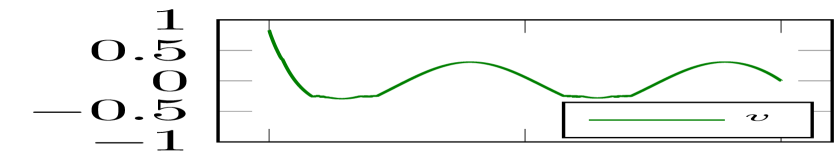
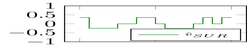
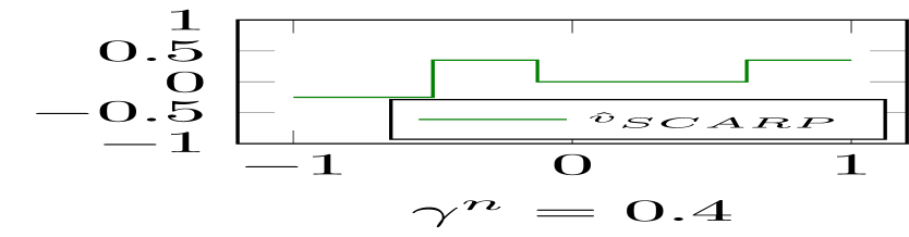
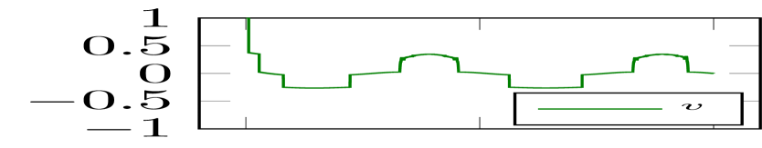
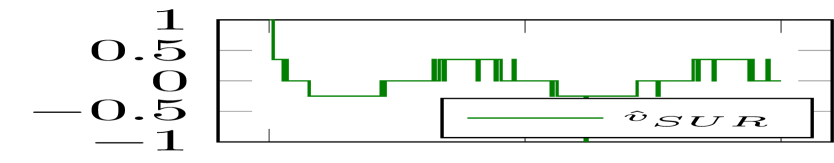
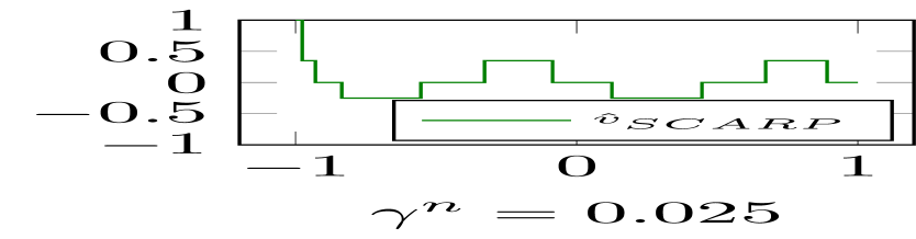
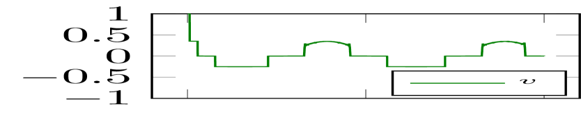
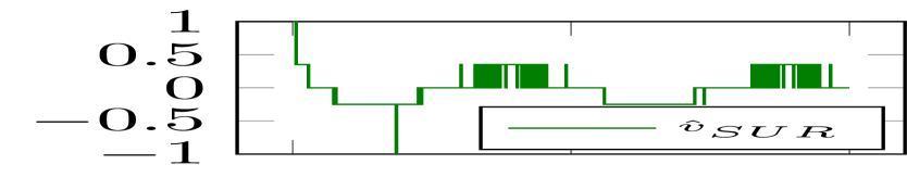
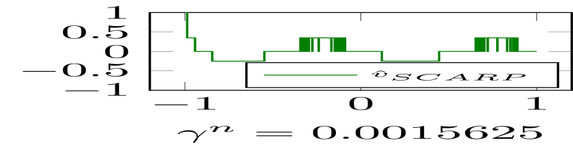
Figure 3: Computed controls in iterations $n=1$,$5$,$9$ (left to right) in ln. 3 (top) and in ln. 13 for SUR (center) and SCARP (bottom).

4.2 Lotka–Volterra Problem

The Lotka–Volterra problem [33] with relaxed multibang regularizer for a two-dimensional discrete control input is

$$\begin{aligned} \inf_{y,v}\ &\int_{t_{0}}^{t_{f}}\left\|y(t)-\begin{pmatrix}1&1\end{pmatrix}^{T}\right\|_{2}^{2}+\eta\int_{t_{0}}^{t_{f}}g(v(t))\,\mathop{}\!\mathrm{d}t\eqqcolon J(v)\\ \text{s.t.}\ &\left\{\begin{aligned} \dot{y}_{1}(t)&=y_{1}(t)-y_{1}(t)y_{2}(t)-y_{1}(t)v_{1}(t)\text{ for a.a.\ }t\in(t_{0},t_{f}),\\ \dot{y}_{2}(t)&=-y_{2}(t)+y_{1}(t)y_{2}(t)-y_{2}(t)v_{2}(t)\text{ for a.a.\ }t\in(t_{0},t_{f}),\\ y(t_{0})&=\begin{pmatrix}0.5&0.7\end{pmatrix}^{T},\\ v(t)&\in\left\{\nu_{1},\nu_{2},\nu_{3},\nu_{4},\nu_{5}\right\}\text{ for a.a.\ }t\in(t_{0},t_{f}),\end{aligned}\right.\end{aligned}$$ (LVP)

where $t_{0}=0$, $t_{f}=12$, $\nu_{1}=\begin{pmatrix}0&-0.1\end{pmatrix}^{T}$, $\nu_{2}=\begin{pmatrix}0.05&0.0\end{pmatrix}^{T}$, $\nu_{3}=\begin{pmatrix}0.4&-0.1\end{pmatrix}^{T}$, $\nu_{4}=\begin{pmatrix}0.0&0.1\end{pmatrix}^{T}$, and $\nu_{5}=\begin{pmatrix}0.4&0.1\end{pmatrix}^{T}$ and $g$ is defined as in Definition 2.4 with $g_{1}=2$, $g_{2}=0$, $g_{3}=1$, $g_{4}=2$, and $g_{5}=0.1$. We choose $\eta=0.005$. We discretize the initial value problem and the objective and solve the continuous relaxation with the software package CasADi [1] with Ipopt [44] as the nonlinear programming solver.

Deriving a closed-form expression for the Moreau envelopes of $g$ is difficult. Therefore, we have computed the values of $g$ and $g_{\gamma}$ on a fine grid that discretizes $\operatorname*{conv}V=[0.0,0.4]\times[-0.1,0.1]$ and interpolated them. Figure 4 shows the function $g$ and its Moreau envelopes $g_{\gamma}$ for the choices $\gamma=5\cdot 10^{-3}$ and $\gamma=10^{-3}$.

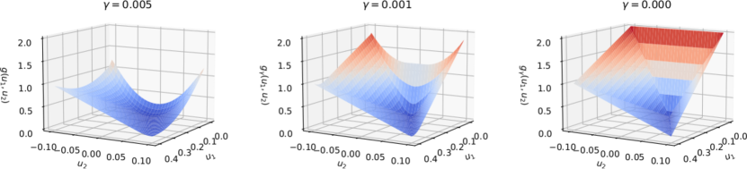
Figure 4: Two-dimensional multibang relaxed regularizer (right) and its Moreau envelopes for $\gamma=5\cdot 10^{-3}$ (left) and $\gamma=10^{-3}$ (center).

The Lotka–Volterra problem may be nonconvex, and we cannot expect more than convergence of the solution of the continuous relaxation to a local minimizer. Therefore, we disregard the global optimality condition implied by Algorithm 1 ln. 3 for this problem. Again, we use SCARP [2, 3] as rounding algorithm in Algorithm 1 and choose $\theta=2$ with respect to Definition 3.5. We mimic driving $\varepsilon^{n}$ to zero by refining the discretization in every iteration. We optimize over piecewise constant ansatz functions for the controls and use the control discretization grid as rounding grid. Therefore, we always have $\|v^{n}-\bar{v}^{n}\|_{L^{2}}=0$.

We have run the algorithm for six iterations. We provide the values of $\Delta^{n}$, $N^{n}$, $\gamma^{n}$ and the relative difference between the overestimator $J(\hat{v}^{n})$ and the underestimator $J_{\gamma^{n}}(v^{n})$ for the current discretization in Table 2. The relative difference tends to zero over the iterations, which indicates that the computed iterates $v^{n}$ of the discretized continuous relaxations tend to a local minimizer and corresponding weak-^∗-convergence of the discrete-valued iterates $\hat{v}^{n}$. The $L^{2}$-difference between relaxed and discrete control $\|v^{n}-\hat{v}^{n}\|_{L^{2}}$ decreases with less smoothing over the iterations, indicating that the relaxed multibang regularizer promotes discrete-valued controls. The relaxed and discrete controls in iterations $2$, $4$ and $6$ are displayed in Figure 5.

Table 2: Output of six iterations of Algorithm 1 applied to (LVP).

Iteration	$N^{n}$	$\Delta^{n}$	$\gamma^{n}$	$\frac{J(\hat{v}^{n})-J_{\gamma^{n}}(v^{n})}{J_{\gamma^{n}}(v^{n})}$	$\|v^{n}-\hat{v}^{n}\|_{L^{2}}$
1	16	7.5000e-01	3.1250e-01	2.9629e+00	4.0609e-01
2	32	3.7500e-01	6.2500e-02	9.5257e-01	4.7660e-01
3	64	1.8750e-01	1.2500e-02	5.0805e-01	3.9329e-01
4	128	9.3750e-02	2.5000e-03	3.9579e-02	2.4475e-01
5	256	4.6875e-02	5.0000e-04	2.4117e-02	2.1208e-01
6	512	2.3438e-02	1.0000e-04	6.9964e-03	1.8743e-01

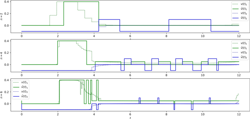
Figure 5: Components ($1$ green, $2$ blue) of the controls $v^{n}$ (dotted) and $\hat{v}^{n}$ (solid) produced by Algorithm 1 in iterations $n=2,4,6$.

5 Conclusion

Relaxed multibang regularizers are suitable for regularizing the integer optimal control problems that can be treated with the combinatorial integral approximation decomposition. They can be integrated in the algorithmic framework, and their nonsmoothness can be alleviated by using Moreau envelopes. Two test problems demonstrate the efficacy of the extended algorithmic framework.

The presented approach can reduce switching costs in practice by promoting $V$-valued controls in (R), which is indicated by the numerical results; also compare Figure 3 with Figure 4 in [22] and consider the results in [9, 10]. Because of the weak-^∗ approximation, high-frequency switching cannot be avoided for fine rounding grids if the (optimal) relaxed control is fractional-valued. Total variation penalties are an intuitive choice to avoid high-frequency switching in optimal control; see also [8]. They cannot be modeled as relaxed multibang regularizers, however; see also [3, Rem. 4]. Switching costs and constraints on dwell times can be included in the second step of the combinatorial integral approximation; see [3, 47]. If switching costs need to be limited a priori, a general theory is not at hand and, in the context of the combinatorial integral approximation, a gap between $\inf\eqref{eq:p}$ and $\min\eqref{eq:r}$ has to be accepted so far. Finally, regularization terms may not always make sense. If the infimal value of the term $F$ needs to be approximated closely and high-frequency switching controls can be generated, then a choice $R\neq 0$ may counteract this goal and increase the lowest achievable value of $F$.

Appendix A Auxiliary Proofs

A.1 Proof of Proposition 1.1

Proof.

Since the Carathéodory conditions are satisfied for $g$, the Nemytskii operator induced by $g$ is a bounded and continuous map from $L^{2}(\Omega,\mathbb{R}^{m})$ to $L^{2}(\Omega)$ and thus $R\in C(L^{2}(\Omega,\mathbb{R}^{m}),[0,\infty))$; see [30, Sect. 10.3.4].

We split $R(\bar{v})$ as follows:

$$R(w)=\int_{A}g(\bar{v}(x))\,\mathop{}\!\mathrm{d}x+\int_{A^{c}}g(\bar{v}(x))\,\mathop{}\!\mathrm{d}x.$$

Let $x\in\Omega$. Let $i\in[M]$ and $n\in\mathbb{N}$. Then, we can define

$$\beta^{n}_{i}(x)\coloneqq\left\{\begin{aligned} 1&\text{ if }v^{n}(x)=\nu_{i},\\ 0&\text{ else}.\end{aligned}\right.$$

Since the $v^{n}$ are measurable, so are the $\beta^{n}$. The sequence $(\beta^{n})_{n}$ is bounded in the space $L^{\infty}(\Omega,\mathbb{R}^{M})$ and thus admits a weakly-^∗-convergent subsequence with limit $\alpha\in L^{\infty}(\Omega,\mathbb{R}^{M})$. Moreover, since $v^{n}=\sum_{i=1}^{M}\beta^{n}_{i}\nu_{i}$, we obtain

$$v^{n}=\sum_{i=1}^{M}\beta^{n}_{i}\nu_{i}\stackrel{{\scriptstyle\ast}}{{\rightharpoonup}}\sum_{i=1}^{M}\alpha^{n}_{i}\nu_{i}=\bar{v},$$

where the last identity follows from the uniqueness of the limit. From the fact that the $\beta^{n}$ are $\{0,1\}^{M}$-valued, we deduce that $0\leq\alpha_{i}(x)$ and $\sum_{i=1}^{M}\alpha^{n}_{i}(x)=1$ for a.a. $x\in\Omega$. In words, $\alpha$ constitutes a vector of convex coefficients a.e. Moreover, the fact that the $\beta^{n}$ are $\{0,1\}^{M}$-valued also implies $g(v^{n}(x))=\sum_{i=1}^{M}\beta^{n}_{i}(x)g(\nu_{i})$ for a.a. $x\in\Omega$.

Thus, we may conclude

$$R(v^{n})=\sum_{i=1}^{M}\int_{\Omega}\beta^{n}_{i}(x)g(\nu_{i})\,\mathop{}\!\mathrm{d}x\to\sum_{i=1}^{M}\int_{\Omega}\alpha_{i}(x)g(\nu_{i})\,\mathop{}\!\mathrm{d}x.$$ (A.1)

Let $D\subset\Omega$ be measurable. Then,

$$\sum_{i=1}^{M}\int_{D}\alpha_{i}(x)g(\nu_{i})\,\mathop{}\!\mathrm{d}x\geq\int_{D}g(\bar{v}(x))\,\mathop{}\!\mathrm{d}x$$ (A.2)

because $\alpha$ constitutes a vector of convex coefficients a.e., and $g$ is convex.

Now, we note that $\alpha(x)\notin\{0,1\}^{M}$ for a.a. $x\in A$ because $\bar{v}(x)\in\operatorname*{conv}V\setminus V$ for a.a. $x\in A$. We show that there exists $\varepsilon>0$ such that

$$\sum_{i=1}^{M}\alpha_{i}(x)g(\nu_{i})>g\left(\sum_{i=1}^{M}\alpha_{i}(x)\nu_{i}\right)+\varepsilon=g(\bar{v}(x))+\varepsilon$$

for all $x\in B$ for a set $B\subset A$ such that $\lambda(B)>0$. To see this, we assume the converse and obtain that

$$\sum_{i=1}^{M}\alpha_{i}(x)g(\nu_{i})=g\left(\sum_{i=1}^{M}\alpha_{i}(x)\nu_{i}\right)=g(\bar{v}(x))$$

holds for a.a. $x\in A$. But since $g$ is strictly convex, this means that $\alpha(x)\in\{0,1\}^{M}$ for a.a. $x\in A$, which is a contradiction.

We conclude that

$$\int_{B}\sum_{i=1}^{M}\alpha_{i}(x)g(\nu_{i})>\int_{B}g(w(x))\,\mathop{}\!\mathrm{d}x+\varepsilon\lambda(B).$$

Combining this estimate with (A.2) for the choice $D=B^{c}$ and inserting both estimates into (A.1), we get

$$\liminf R(v^{n}) =\sum_{i=1}^{M}\int_{B^{c}}\alpha_{i}(x)g(\nu_{i})\,\mathop{}\!\mathrm{d}x+\sum_{i=1}^{M}\int_{B}\alpha_{i}(x)g(\nu_{i})\,\mathop{}\!\mathrm{d}x$$

$$>\int_{B^{c}}g(\bar{v}(x))\,\mathop{}\!\mathrm{d}x+\int_{B}g(\bar{v}(x))\,\mathop{}\!\mathrm{d}x+\varepsilon\lambda(B)$$

$$>\int_{\Omega}g(\bar{v}(x))\,\mathop{}\!\mathrm{d}x.$$

This concludes the proof. ∎

We note that the Lyapunov convexity theorem (see [25, 41]) asserts that such a sequence $(v^{n})_{n}$ exists for all functions $\bar{v}$ as in Proposition 1.1.

A.2 Proof of (2.8)

Proof.

Let $w\in\mathcal{F}_{\eqref{eq:r}}$ and $\gamma>0$ be given. Then, we obtain

$$R(w)-R_{\gamma}(w)=\int_{\Omega}d(w(x))\,\mathop{}\!\mathrm{d}x$$ (A.3)

with

$$d(u)\coloneqq g(u)-\inf\left\{g(y)+\frac{1}{2\gamma}\|u-y\|^{2}_{2}\,\Big{|}\,y\in\operatorname*{conv}\{\nu_{1},\ldots,\nu_{M}\}\right\}.$$

For $u\in\operatorname*{conv}\{\nu_{1},\ldots,\nu_{M}\}$, we consider $d(u)$ and rewrite it as

$$d(u)=\sup\left\{g(u)-g(y)-\frac{1}{2\gamma}\|u-y\|^{2}_{2}\,\Big{|}\,y\in\operatorname*{conv}\{\nu_{1},\ldots,\nu_{M}\}\right\}.$$

Proposition 2.5 2 gives that $g$ is Lipschitz continuous with constant $L$, and we obtain

$$d(u)\leq\sup\left\{L\|u-y\|_{2}-\frac{1}{2\gamma}\|u-y\|^{2}_{2}\,\Big{|}\,y\in\operatorname*{conv}\{\nu_{1},\ldots,\nu_{M}\}\right\}\leq\frac{L^{2}\gamma}{2},$$

where the second inequality follows from the maximization of a parabola with negative curvature. Inserting this estimate into (A.3) yields (2.8). ∎

Appendix B Alternative Smoothing in the One-Dimensional Case

Let $R$ be a relaxed multibang regularizer for discrete- and scalar-valued controls; that is, $R(v)\coloneqq\int_{\Omega}g(v(x))\,\mathop{}\!\mathrm{d}x$ for control functions $v\in\mathcal{F}_{\eqref{eq:r}}$. Here, we consider the set of feasible controls for (R):

$$\mathcal{F}_{\eqref{eq:r}}=\{v\in L^{2}(\Omega)\,|\,v(x)\in[\nu_{1},\nu_{M}]\text{ for a.a.\ }x\in\Omega\}$$

with scalars $\nu_{1}<\ldots<\nu_{M}$. We assume that $g:[\nu_{1},\nu_{M}]\to\mathbb{R}$ is a positive, continuous, montonously increasing, piecewise affine convex function with $g(\nu_{1})=0$ and that $g(\nu_{M})=B\in\mathbb{R}$.

It is straightforward to generalize the following ideas if the monotonicity assumption is dropped or $g(\nu_{1})$ is allowed to be nonzero; but this restriction simplifies the remainder significantly, and we believe that it also helps to get a good intuition.

The Clarke subdifferential $\partial^{c}g$ of $g$ is

$$\partial^{c}g(u)=\left\{\begin{aligned} \{L_{1}\}&\text{ if }u=\nu_{1},\\ \{L_{i}\}&\text{ if }u\in(\nu_{i},\nu_{i+1})\text{ for some }i\in[M-1],\\ \{L_{M-1}\}&\text{ if }u=\nu_{M},\\ [L_{i-1},L_{i}]&\text{ if }u=\nu_{i}\text{ for some }i\in[M-1]\end{aligned}\right.$$

for positive slopes $0<L_{1}<\ldots<L_{M-1}$. We observe that $\partial^{c}g$ is almost everywhere single-valued. Thus, we may interpret $\partial^{c}g$ as an $L^{\infty}$-function, which we denote by $g^{\prime}$ because for this $L^{\infty}$-function we still have $g(u)=\int_{\nu_{1}}^{u}g^{\prime}(w)\,\mathop{}\!\mathrm{d}w$ by the fundamental theorem of Lebesgue integral calculus. In other words, the function $g$ is absolutely continuous. For $v\in\mathcal{F}_{\eqref{eq:r}}$, we have $g(v(x))\leq B$ for a.a. $x\in\Omega$, and thus $R(v)\leq B\lambda(\Omega)$. For $i\in[M]$, we define $g_{i}\coloneqq g(\nu_{i})$.

Now, we define differentiable convex underestimators of $g$. We define the $C^{1}\cap W^{2,\infty}$-function $g_{\gamma}:[\nu_{1},\nu_{M}]\to\mathbb{R}$

$$g_{\gamma}(u)\coloneqq\int_{\nu_{1}}^{u}g^{\prime}_{\gamma}(w)\,\mathop{}\!\mathrm{d}w\text{ for }u\in[\nu_{1},\nu_{M}]$$

for $0<\gamma<\min\{\nu_{i+1}-\nu_{i}\,|\,i\in[M-1]\}$, where $g_{\gamma}^{\prime}$ is defined as

$$g_{\gamma}^{\prime}(w)\coloneqq\left\{\begin{aligned} L_{1}&\text{ if }w\in[\nu_{1},\nu_{2}),\\ L_{i-1}+\frac{L_{i}-L_{i-1}}{\gamma}(s-\nu_{i})&\text{ if }w\in[\nu_{i},\nu_{i}+\gamma)\text{ for some }i\in[M-1]\setminus\{1\},\\ L_{i}&\text{ if }w\in[\nu_{i}+\gamma,\nu_{i+1})\text{ for some }i\in[M-1],\\ L_{M-1}&\text{ if }w=\nu_{M}\end{aligned}\right.$$

for all $w\in[\nu_{1},\nu_{M}]$. We show an example for $g$ with underestimators and their derivatives in Figure 6.

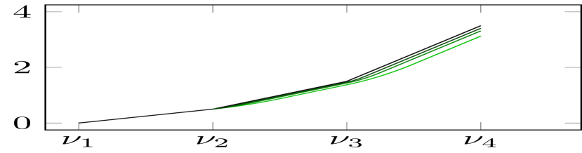
(a) $g$ (black) and approximations $g_{\gamma}$.

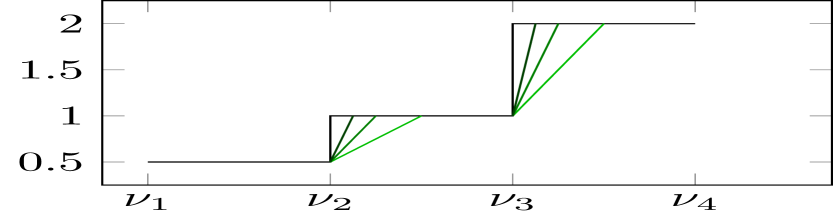
(b) $\partial^{c}g$ (black) and approximations $g_{\gamma}^{\prime}$.

Figure 6: $g$ and $\partial^{C}g$ as well as their approximations $g_{\gamma}$ and $g_{\gamma}^{\prime}$ for the choices $\gamma\in\{2^{-1},2^{-2},2^{-3}\}$.

Following our notation, we define the smoothed regularizer as

$$R_{\gamma}(v)\coloneqq\int_{\Omega}g_{\gamma}(v(x))\,\mathop{}\!\mathrm{d}x$$ (B.1)

for all $v\in\mathcal{F}_{\eqref{eq:r}}$. We summarize the properties of the relatonship between $g_{\gamma}$ and $g$ in the proposition below.

Proposition B.1.

Let $0<\gamma<\min\{\nu_{i+1}-\nu_{i}\,|\,i\in[M-1]\}$. It holds that

$$\begin{aligned} \left\|g-g_{\gamma}\right\|_{C([0,T])}&=0.5(L_{M-1}-L_{1})\gamma,\\ \left\|g^{\prime}-g^{\prime}_{\gamma}\right\|_{L^{1}([0,T])}&=0.5(L_{M-1}-L_{1})\gamma,\\ \left\|g^{\prime}-g^{\prime}_{\gamma}\right\|_{L^{p}([0,T])}&=\left(\sum_{i=1}^{M-2}(L_{i+1}-L_{i})^{p}\frac{p}{p+1}\gamma\right)^{\frac{1}{p}}\text{ for }p\in(1,\infty),\\ \|g^{\prime}-g_{\gamma}^{\prime}\|_{L^{\infty}([0,T])}&=\max\{L_{i+1}-L_{i}\,|\,i\in[M-2]\}.\end{aligned}$$

Proof.

By construction of $g_{\gamma}$, we have $g(u)\geq g_{\gamma}(u)$ for all $u\in[\nu_{1},\nu_{M}]$. We consider the difference $d_{\gamma}(u)\coloneqq g(u)-g_{\gamma}(u)$ for $u$ in different intervals. For $i\in[M]$, let $d_{\gamma}^{i}\coloneqq g(\nu_{i})-g_{\gamma}(\nu_{i})$.

Because $g(u)=g_{\gamma}(u)$ for all $u\in[\nu_{1},\nu_{2}]$ it holds that $d_{\gamma}^{1}=d_{\gamma}^{2}=0$. Let $i\in\{2,\ldots,M-1\}$. For $u\in[\nu_{i},\nu_{i+1}]$ it holds that

$$d_{\gamma}(u) =d_{\gamma}^{i}+\int_{\nu_{i}}^{\min\{u,\nu_{i}+\gamma\}}L_{i}-L_{i-1}-\left(\frac{L_{i}-L_{i-1}}{\gamma}\right)(w-\nu_{i})\,\mathop{}\!\mathrm{d}w$$

$$=d_{\gamma}^{i}+(L_{i}-L_{i-1})\min\{u-\nu_{i},\gamma\}-\frac{L_{i}-L_{i-1}}{2\gamma}\min\{u-\nu_{i},\gamma\}^{2}.$$

Thus, $d_{\gamma}$ is a continuous montonously nondecreasing function, and we obtain $\sup_{u}d_{\gamma}(u)=d_{\gamma}(\nu_{M})$. Using the iterative description of $d_{\gamma}$ derived above and the assumption $\gamma<\min\{\nu_{i+1}-\nu_{i}\,|\,i\in[M-1]\}$, we can compute

$$d_{\gamma}(\nu_{M})=\sum_{i=1}^{M-2}(L_{i+1}-L_{i})\gamma-\frac{L_{i+1}-L_{i}}{2\gamma}\gamma^{2}=\frac{L_{M-1}-L_{1}}{2}\gamma.$$

This implies $\|g-g_{\gamma}\|_{C}=0.5(L_{M-1}-L_{1})\gamma$. Since $g^{\prime}\geq g_{\gamma}^{\prime}$ almost everywhere, it also holds that $\|g^{\prime}-g_{\gamma}^{\prime}\|_{L^{1}}=0.5(L_{M-1}-L_{1})\gamma$. Let $p\in(1,\infty)$. Then a reasoning similar to the above yields

$$\|g^{\prime}-g_{\gamma}^{\prime}\|_{L^{p}([\nu_{1},\nu_{M}])}=\left(\sum_{i=1}^{M-2}(L_{i+1}-L_{i})^{p}\frac{p}{p+1}\gamma\right)^{\frac{1}{p}}.$$

By construction $\|g^{\prime}-g^{\prime}_{\gamma}\|_{L^{\infty}([\nu_{1},\nu_{2}])}=0$ and $\|g^{\prime}-g^{\prime}_{\gamma}\|_{L^{\infty}([\nu_{i},\nu_{i+1}])}=L_{i}-L_{i-1}$ for all $i\in\{2,M-1\}$, which yields the last claim. ∎

We obtain the following corollary, which establishes the properties of the Moreau envelope from Proposition 2.14 for $R_{\gamma}$ and $g_{\gamma}$ as well.

Corollary B.2.

1. For all $u\in\operatorname*{conv}V$ it holds that $g_{\gamma}(u)\uparrow g(u)$ for $\gamma\downarrow 0$.

2. For all $v\in\mathcal{F}_{\eqref{eq:r}}$ it holds that $R_{\gamma}(v)\uparrow R(v)$ for $\gamma\downarrow 0$.

3. For all $\gamma>0$, the function $g_{\gamma}:\operatorname*{conv}V\to\mathbb{R}$ is convex and continuously differentiable with Lipschitz-continuous derivative.

4. Let $p\geq 2$. Then, $R_{\gamma}:L^{p}(\Omega,\mathbb{R}^{m})\to\mathbb{R}$ is differentiable with derivative $R_{\gamma}^{\prime}(v)d=\int_{\Omega}g_{\gamma}^{\prime}(v(x))^{T}d(x)\,\mathop{}\!\mathrm{d}x$.

Proof.

The claims follow along the lines of the proof of Proposition 2.14. ∎

Proposition B.3.

Let $(\gamma^{n})_{n}\subset[0,\infty)$ satisfy $\gamma^{n}\downarrow 0$. Then, the sequence of functionals $F+R_{\gamma^{n}}$ on $\mathcal{F}_{\eqref{eq:r}}\subset L^{\infty}(\Omega,\mathbb{R}^{m})$ is $\Gamma$-convergent with limit $F+R$ with respect to weak-^∗-convergence in $L^{\infty}$.

Proof.

The claim follows along the lines of the proof of Proposition 2.15. The estimates on $g-g_{\gamma}$ can be taken directly from Proposition B.1. ∎

Theorem B.4.

Let $R$ be a relaxed multibang regularizer. Let the inputs of Algorithm 1 be given. Let $\nu_{1}<\ldots<\nu_{M}$. Then, the assertions of Theorem 3.8 hold true if the smoothing of $R$ is performed as defined in (B.1) instead of using the Moreau envelope.

Proof.

This follows along the lines of the proof of Theorem 3.8 with the considerations above to replace the estimates on the Moreau envelope. ∎

Government License

The submitted manuscript has been created by UChicago Argonne, LLC, Operator of Argonne National Laboratory (“Argonne”). Argonne, a U.S. Department of Energy Office of Science laboratory, is operated under Contract No. DE-AC02-06CH11357. The U.S. Government retains for itself, and others acting on its behalf, a paid-up nonexclusive, irrevocable worldwide license in said article to reproduce, prepare derivative works, distribute copies to the public, and perform publicly and display publicly, by or on behalf of the Government. The Department of Energy will provide public access to these results of federally sponsored research in accordance with the DOE Public Access Plan http://energy.gov/downloads/doe-public-access-plan.

References

- [1] J. A. E. Andersson, J. Gillis, G. Horn, J. B. Rawlings, and M. Diehl. CasADi – A software framework for nonlinear optimization and optimal control. Mathematical Programming Computation, 11(1):1–36, 2019.
- [2] F. Bestehorn, C. Hansknecht, C. Kirches, and P. Manns. A switching cost aware rounding method for relaxations of mixed-integer optimal control problems. In 2019 IEEE 58th Conference on Decision and Control (CDC), pages 7134–7139. IEEE, 2019.
- [3] Felix Bestehorn, Christoph Hansknecht, Christian Kirches, and Paul Manns. Mixed-integer optimal control problems with switching costs: a shortest path approach. Mathematical Programming, pages 1–32, 2020.
- [4] Volker Böhm. On the continuity of the optimal policy set for linear programs. SIAM Journal on Applied Mathematics, 28(2):303–306, 1975.
- [5] T. Borrvall and J. Petersson. Topology optimization using regularized intermediate density control. Computer Methods in Applied Mechanics and Engineering, 190(37-38):4911–4928, 2001.
- [6] M. A. Branch, T. F. Coleman, and Y. Li. A subspace, interior, and conjugate gradient method for large-scale bound-constrained minimization problems. SIAM Journal on Scientific Computing, 21(1):1–23, 1999.
- [7] C. Buchheim, A. Caprara, and A. Lodi. An effective branch-and-bound algorithm for convex quadratic integer programming. Mathematical Programming, 135(1-2):369–395, 2012.
- [8] C. Clason, F. Kruse, and K. Kunisch. Total variation regularization of multi-material topology optimization. ESAIM: Mathematical Modelling and Numerical Analysis, 52(1):275–303, 2018.
- [9] C. Clason and K. Kunisch. Multi-bang control of elliptic systems. In Annales de l’Institut Henri Poincaré (c) Analysé Non Linéaire, volume 31, pages 1109–1130. Elsevier, 2014.
- [10] C. Clason and K. Kunisch. A convex analysis approach to multi-material topology optimization. ESAIM: Mathematical Modelling and Numerical Analysis, 50(6):1917–1936, 2016.
- [11] C. Clason, C. Tameling, and B. Wirth. Vector-valued multibang control of differential equations. SIAM Journal on Control and Optimization, 56(3):2295–2326, 2018.
- [12] G. Dal Maso. An Introduction to -Convergence, volume 8. Birkhäuser Basel, 1993.
- [13] I. Fonseca and G. Leoni. Modern Methods in the Calculus of Variations: Lp Spaces. Springer Science & Business Media, 2007.
- [14] D. Garmatter, M. Porcelli, F. Rinaldi, and M. Stoll. Improved penalty algorithm for mixed integer pde constrained optimization (mipdeco) problems. arXiv preprint arXiv:1907.06462, 2019.
- [15] Helmuth Goldberg, Winfried Kampowsky, and Fredi Tröltzsch. On Nemytskij operators in Lp-spaces of abstract functions. Mathematische Nachrichten, 155(1):127–140, 1992.
- [16] F. M. Hante and S. Sager. Relaxation methods for mixed-integer optimal control of partial differential equations. Computational Optimization and Applications, 55(1):197–225, 2013.
- [17] J. Haslinger and R. A. E. Mäkinen. On a topology optimization problem governed by two-dimensional helmholtz equation. Computational Optimization and Applications, 62(2):517–544, 2015.
- [18] C. J. Himmelberg, T. Parthasarathy, and F. S. Van Vleck. Optimal plans for dynamic programming problems. Mathematics of Operations Research, 1(4):390–394, 1976.
- [19] M. Jung. Relaxations and approximations for mixed-integer optimal control. PhD thesis, Heidelberg University, 2013.
- [20] M. N. Jung, G. Reinelt, and S. Sager. The Lagrangian relaxation for the combinatorial integral approximation problem. Optimization Methods and Software, 30(1):54–80, 2015.
- [21] C. Kirches, F. Lenders, and P. Manns. Approximation properties and tight bounds for constrained mixed-integer optimal control. SIAM Journal on Control and Optimization, 58(3):1371–1402, 2020.
- [22] C. Kirches, P. Manns, and S. Ulbrich. Compactness and convergence rates in the combinatorial integral approximation decomposition. Mathematical Programming, pages 1–30, 2020.
- [23] K. Kuratowski and C. Ryll-Nardzewski. A general theorem on selectors. Bull. Acad. Polon. Sci., Sér. Math. Astronom. Phys., 13(6):397–403, 1965.
- [24] S. Leyffer, P. Manns, and M. Winckler. Convergence of sum-up rounding schemes for cloaking problems governed by the helmholtz equation. Computational Optimization and Applications, pages 1–29, 2021.
- [25] A. A. Lyapunov. On completely additive vector functions. Izv. Akad. Nauk SSSR, 4:465–478, 1940.
- [26] O. L. Mangasarian and T-H Shiau. Lipschitz continuity of solutions of linear inequalities, programs and complementarity problems. SIAM Journal on Control and Optimization, 25(3):583–595, 1987.
- [27] P. Manns and C. Kirches. Improved regularity assumptions for partial outer convexification of mixed-integer pde-constrained optimization problems. ESAIM: Control, Optimisation and Calculus of Variations, 26:32, 2020.
- [28] P. Manns, C. Kirches, and F. Lenders. Approximation properties of sum-up rounding in the presence of vanishing constraints. Mathematics of Computation, 2020. (accepted).
- [29] Paul Manns and Christian Kirches. Multidimensional sum-up rounding for elliptic control systems. SIAM Journal on Numerical Analysis, 58(6):3427–3447, 2020.
- [30] M. Renardy and R. C. Rogers. An introduction to partial differential equations, volume 13. Springer Science & Business Media, 2006.
- [31] R. T. Rockafellar and R. J. B. Wets. Variational Analysis. Springer, Berlin, 2004.
- [32] S. Sager. Numerical methods for mixed-integer optimal control problems. Der andere Verlag Tönning, Lübeck, Marburg, 2005.
- [33] S. Sager. A benchmark library of mixed-integer optimal control problems. In Mixed Integer Nonlinear Programming, pages 631–670. Springer, 2012.
- [34] S. Sager. Sampling decisions in optimum experimental design in the light of Pontryagin’s maximum principle. SIAM Journal on Control and Optimization, 51(4):3181–3207, 2013.
- [35] S. Sager, H.-G. Bock, and M. Diehl. The Integer Approximation Error in Mixed-Integer Optimal Control. Mathematical Programming, Series A, 133(1–2):1–23, 2012.
- [36] S. Sager, H. G. Bock, M. Diehl, G. Reinelt, and J. P. Schlöder. Numerical methods for optimal control with binary control functions applied to a lotka-volterra type fishing problem. In Recent Advances in Optimization, pages 269–289. Springer, 2006.
- [37] S. Sager, M. Jung, and C. Kirches. Combinatorial integral approximation. Mathematical Methods of Operations Research, 73(3):363–380, 2011.
- [38] Meenarli Sharma, Mirko Hahn, Sven Leyffer, Lars Ruthotto, and Bart van Bloemen Waanders. Inversion of convection–diffusion equation with discrete sources. Optimization and Engineering, pages 1–39, 2020.
- [39] G. Stadler. Elliptic optimal control problems with L1-control cost and applications for the placement of control devices. Computational Optimization and Applications, 44(2):159, 2009.
- [40] E. M. Stein and R. Shakarchi. Real analysis: measure theory, integration, and Hilbert spaces. Princeton University Press, 2005.
- [41] L. Tartar. Compensated compactness and applications to partial differential equations. In Nonlinear analysis and mechanics: Heriot-Watt symposium, volume 4, pages 136–212, 1979.
- [42] P. Virtanen, R. Gommers, T. E. Oliphant, M. Haberland, T. Reddy, D. Cournapeau, E. Burovski, P. Peterson, W. Weckesser, J. Bright, S. J. van der Walt, M. Brett, J. Wilson, K. Jarrod Millman, N. Mayorov, A. R. J. Nelson, E. Jones, R. Kern, . . . , P. van Mulbregt, and . . Contributors. SciPy 1.0: Fundamental Algorithms for Scientific Computing in Python. Nature Methods, 17:261–272, 2020.
- [43] C. Voglis and I. E. Lagaris. A rectangular trust region dogleg approach for unconstrained and bound constrained nonlinear optimization. In WSEAS 6th International Conference on Applied Mathematics, pages 1–7, 2004.
- [44] A. Wächter and L. T. Biegler. On the implementation of an interior-point filter line-search algorithm for large-scale nonlinear programming. Mathematical Programming, 106(1):25–57, 2006.
- [45] Jing Yu and Mihai Anitescu. Multidimensional sum-up rounding for integer programming in optimal experimental design. Mathematical Programming, pages 1–40, 2019.
- [46] C. Zeile, T. Weber, and S. Sager. Combinatorial integral approximation decompositions for mixed-integer optimal control. Optimization Online Preprint 6472, 2018.
- [47] Clemens Zeile, Nicolò Robuschi, and Sebastian Sager. Mixed-integer optimal control under minimum dwell time constraints. Mathematical Programming, pages 1–42, 2020.