Analytical model of millisecond pulsar PSR J0514 - 4002A

Abstract

We construct a relativistic model for the newly discovered millisecond pulsar PSR J0514 - 4002A located in the globular cluster NGC 1851 (A. Ridolfi, P.C.C. Freire, Y. Gupta, S.M. Ransom, MNRAS 490, 3860 (2019)) by using Tolman VII spacetime. We have obtained central density ($\rho_{0}$), central pressure ($p_{0}$), probable radius, compactness ($u$) and surface redshift ($Z_{s}$) of the above mentioned newly discovered millisecond pulsar, which is very much consistent with reported data. Equation of State (EoS) of the millisecond pulsar has comes out as stiff in nature which is physically acceptable. Not even that our proposed model can analyze most of the millisecond pulsars having masses up to $1.51M_{\odot}$.

1 Introduction

The low-mass X-ray binaries (LMXBs) are binary systems in which a neutron star or a black hole accretes matter from a low-mass companion star. These systems(LMXBs) provide a laboratory to test the behavior of matter under extreme physical conditions that are unavailable on Earth. The reprocessed X-ray emission in the outer accretion disc, which is formed around the compact object, dominates the optical flux thereby overflowing any intrinsic spectral feature of the donor star Cornelisse2013 . The Millisecond pulsars (MSPs) are thought to be the offspring of low-mass X-ray binaries (LMXBs) in which mass transfer from a low-mass companion star to the neutron star carries angular momentum and spins it up to a very fast rotation Alpar1982 . When the rate of mass transfer decreases in the later evolutionary stages, these binaries host a radio millisecond pulsar Backer1982 ; Ruderman1989 . At the end of their spin-up phase they are reactivated as rotation-powered (radio and $\gamma$-ray loud) pulsars. In the year 1993, Rotation-powered MSPs were identified as pulsed X-ray sources Becker1993 . The Millisecond pulsars (MSPs) are apparently long aged and emit optical, X-ray and $\gamma$-ray fluxes significantly below from the awaited canonical pulsars with similar periods. The first MSP B1937+214, by the definition of fast accretion spun-up pulsar was discovered using the Arecibo telescope in 1982 Backer1982 . A number of recently discovered millisecond pulsars (MSPs), which lie in binary systems with evolved companion (neutron star), tend to be lighter than the companion due to reduced mass transfer Antoniadis2016 . The study of Millisecond pulsars (MSPs) takes much attention to the astrophysicists in the present decades Zilles2020 ; Voisin2020 ; Gusinskaia2020 ; Vivekanand2019 ; Bogdanov2019 ; Riley2019 ; Bult2019 ; Webb2019 . This study is very important in the physical as well as in theoretical point of view. Scientists used different techniques (such as observational, computational or theoretical analysis) to study the physical properties of astrophysical compact objects like MSPs. The small size massive compact objects like white dwarfs, neutron stars, pulsars, MSPs or black hole, has high dense configurations which influence researchers to obtain models that describe compact objects in the regime of strong gravitational field.

General Relativity describes the gravitational interaction and its consequences very well in a four-dimensional spacetime and it has been confirmed by Will Will2005 with observational and experimental support. The Einstein’s theory of general relativity laid the foundation of our understanding of compact stars. The exact solution of Einstein’s field equations was first solved by Schwarzschild Schwarzschild1916 in 1916. He had calculated the gravitational field of a homogeneous sphere of finite radius, which consists of incompressible fluid. In 1939,Oppenheimer, Volkoff and Tolman Oppenheimer1939 ; Tolman1939 successfully derived the balancing equations of relativistic stellar structures from Einstein’s field equations and they discovered the limit to the mass of a stable relativistic incompressible fluid sphere. With the discovery of pulsars, it was the demand from the scientific community to study neutron stars to build up a connecting bridge between theoretical and observational physics. Compact star models give interesting results in term of the important parameters like stability factor, compactness, red-shift, equation of state etc. which cannot be inferred from direct observation. We suggest to see the details work carried out by many researchers Rahaman2012a ; Rahaman2012b ; Kalam2012a ; Hossein2012 ; Kalam2012b ; Kalam2013 ; Kalam2014 ; Kalam2014a ; Hossein2016a ; Hossein2016b ; Kalam2016 ; Kalam2017 ; Kalam2018 ; Molla2019 ; Islam2019 ; Hendi2016 ; Hendi2017 ; Panah2017 ; Ngubelanga2015 ; Paul2015 ; Lobo2006 ; Bronnikov2006 ; Egeland2007 ; Dymnikova2002 on compact stars.

Tolman Tolman1939 proposed an static solutions for a fluid sphere. He pointed out that due to some complexity of the VII-th solution (among the eight different solutions), it is not possible to explain the physical behavior of a star. We have some curiosities about these conclusion. We thought this solution may explore some physics to compact stars. Several studies have been done on compact stars by many researchers using the Tolman VII-th solution till now. Among them, Neary, Ishak and Lake Neary2001 have found that apart from the exact static spherically symmetric perfect fluid solution, Tolman VII solution exhibits a surprising good approximation for neutron star. The Tolman VII solution is the first exact causal solution which has shown to exhibits trapped null orbits for a tenuity (total radius to mass ratio) $>3$. Thomas E. Kiess Kiess2012 derived an exact Einstein-Maxwell metric for a static spherically symmetric perfect fluid with mass and charge. Addition of modest charge to a neutral star enables it to have a larger total mass, a different radius and a larger red-shift. Raghoonundun and Hobill Raghoonundun2015 had deduced for the first time a closed form class of equation of states (EoSs) for neutron stars by using Tolman VII solution. The EoSs allow further analysis of it, leading to a viable model for compact stars with arbitrary surface mass density. It also obeys the stability criteria. Bhar et al. Piyali2015 have studied the behavior of static spherically symmetric relativistic stellar objects with locally anisotropic matter distribution considering the Tolman VII spacetime. They have analyzed different physical properties of the stellar model and presented it graphically. Singh et al. Singh2016 have presented a new exact solution of charged anisotropic Tolman VII type solution representing compact stars. According to them, this solution can be used to model both neutron star and quark star within the range of observed masses and radii. Bhar et al. Piyali2017 also have studied compact star in Tolman VII spacetime with quadratic equation of state of matter distribution.Using their solution, they optimized the masses and radii of few well-known compact stars within the limit of their observed values. Sotani and Kokkotas Sotani2018 have systematically examine the compactness of neutron stars using Tolman VII solutions in scalar-tensor theory of gravity. They showed that the maximum compactness of neutron stars in general relativity is higher than that in scalar-tensor gravity when the coupling constant is confined to values provided by astronomical observations. Hensh and Stuchlík Hensh2019 have started from the isotropic Tolman VII perfect fluid solution and by using the MGD method they have got a new exact and analytical solution. This new solution represents the anisotropic version of the Tolman VII solution, which satisfies all criteria for physical acceptability. Hence, they argued that this new solution could be used to model of stellar configurations, like neutron stars. They demonstrate that the effect of anisotropy will increase with the increases in coupling constant($\alpha$).

Ridolfi et al. Ridolfi2019 very recently reported the results of one year of upgraded Giant Metrewave Radio Telescope timing measurements of PSR J0514-4002A, a 4.99-ms pulsar in a 18.8-day, eccentric (e = 0.89) orbit with a massive companion located in the globular cluster NGC 1851. They greatly improve the precision of the rate of advance of periastron, $\dot{\omega}$ = 0.0129592(16) deg $yr^{-1}$ by combining these timing measurements data with the earlier Green Bank Telescope data. As a result, a much refine measurement of the total mass $M_{tot}=2.4730(6)M_{\odot}$ of the binary has been done. They also measured the Einstein delay parameter,$\gamma$ = 0.0216(9)s for this binary pulsar which has never been done for any binary system with an orbital period larger than $\sim$ 10 h. Besides, they measured the proper motion of the system ($\mu_{\alpha}=5.19(22)$ & $\mu_{\delta}=-0.56(25)$ mas $yr^{-1}$), which is not only important for analyzing its motion in the cluster, but also essential for a proper interpretation of $\gamma$. They obtained one of the lowest ever measured a pulsar mass of $M_{p}=1.25^{+0.05}_{-0.06}M_{\odot}$ and a companion mass of $M_{c}=1.22^{+0.06}_{-0.05}M_{\odot}$. They guessed that the companion may be a neutron star.

In 2016, Reardon et al. Reardon2016 has measured the mass of PSR J0437-4715 as $1.44\pm 0.07M_{\odot}$. After approximately 2 years of observations with the Caltech-Parkes-Swinburne Recorder II, Jacoby et al. Jacoby2005 precisely measured millisecond pulsar PSR J1909-3744 mass as $1.438\pm 0.024M_{\odot}$. Nice et al. in 2008 Nice2008 and Fortin et al. in 2016 Fortin2016 has also reported the mass of millisecond pulsar PSR J0751+1807 as $1.26\pm 0.14M_{\odot}$.

In this paper, we want to study the physical behaviour of the newly discovered millisecond pulsar PSR J0514-4002A. For this we have considered the anisotropic model to study the fluid sphere. Our main objective in this study is to give an estimate of the equation of state(EoS) of nuclear matter as well as the possible radius of the newly discovered millisecond pulsar PSR J0514-4002A.

We organize the article as follows: In Sec. 2, we have discussed the interior spacetime; density, pressure behavior and EoS of the millisecond pulsar. In Sec. 3, we have studied some special features like: Exterior spacetime and matching condition, Generalized TOV equation, Energy conditions, Stability, Compactness and Surface red-shift in different sub-sections. In Sec. 4, we have concluded our discussion with numerical data.

2 Interior spacetime and Equation of State

Being inspired from many previously revealed famous articles Takisa2019 ; Matondo2018 ; Maurya2015 ; Maurya2019 ; Dayanandana2017 ; Maurya2017 ; Gedela2018 ; Singh2017 ; Jafry2017 ; Rahaman2017 ; Jasim2016 ; Takisa2016 ; Maurya2016 ; Singh2017a , we have taken static, spherical symmetric metric for this pulsar as:

$$ds^{2}=-e^{\nu(r)}dt^{2}+e^{\lambda(r)}dr^{2}+r^{2}(d\theta^{2}+sin^{2}\theta d\phi^{2})$$ (1)

where $\lambda$ and $\nu$ are the functions of radial coordinate(r).
For our model, the form of the energy-momentum tensor is

$$T_{\nu}^{\mu}=(-\rho,p_{r},p_{t},p_{t})$$ (2)

where $\rho$ is the energy density, $p_{r}$ $\&$ $p_{t}$ are the radial and transverse pressure respectively.

Einstein’s field equations for the metric (1) accordingly are obtained as ($c=1,G=1$)

$$8\pi\rho = e^{-\lambda}\left[\frac{\lambda^{\prime}}{r}-\frac{1}{r^{2}}\right]+\frac{1}{r^{2}},$$ (3)

$$8\pi p_{r} = e^{-\lambda}\left[\frac{\nu^{\prime}}{r}+\frac{1}{r^{2}}\right]-\frac{1}{r^{2}}.$$ (4)

$$8\pi p_{t} = \frac{e^{-\lambda}}{2}\left[\nu^{\prime\prime}+\frac{\nu^{\prime}-\lambda^{\prime}}{r}+\frac{{{\nu^{\prime}}^{2}}-{\lambda^{\prime}\nu^{\prime}}}{2}\right]$$ (5)

To solve above Einstein’s field equations we have considered Tolman VII solution as Tolman1939

$$ds^{2}=-B^{2}\sin^{2}\ln\sqrt{\frac{\sqrt{1-\frac{r^{2}}{R^{2}}+4\frac{r^{4}}{A^{4}}}+2\frac{r^{2}}{A^{2}}-\frac{1}{4}\frac{A^{2}}{R^{2}}}{C}}dt^{2}$$

$$+\left(1-\frac{r^{2}}{R^{2}}+4\frac{r^{4}}{A^{4}}\right)^{-1}dr^{2}+r^{2}d\Omega^{2}.~{}~{}~{}~{}~{}~{}~{}~{}~{}~{}$$ (6)

where $R(length)$, $C(dimensionless)$, $A(length)$ and $B$ $(length/time)$ are constants which will be determined later using some physical boundary conditions.
Now from equation (6) we get,

$$e^{-\lambda} = \left(1-\frac{r^{2}}{R^{2}}+4\frac{r^{4}}{A^{4}}\right)$$ (7)

$$\lambda^{\prime} = \frac{\left(2\frac{r}{R^{2}}-16\frac{r^{3}}{A^{4}}\right)}{\left(1-\frac{r^{2}}{R^{2}}+4\frac{r^{4}}{A^{4}}\right)},$$ (8)

$$\nu^{\prime} = \frac{\left(1-\frac{r^{2}}{R^{2}}+4\frac{r^{4}}{A^{4}}\right)^{-1/2}\left(-\frac{r}{2R^{2}}+4\frac{r^{3}}{A^{4}}\right)+2\frac{r}{A^{2}}}{\left(\sqrt{1-\frac{r^{2}}{R^{2}}+4\frac{r^{4}}{A^{4}}}+2\frac{r^{2}}{A^{2}}-\frac{1}{4}\frac{A^{2}}{R^{2}}\right)}$$ (9)

$$2\cot\ln\sqrt{\frac{\sqrt{1-\frac{r^{2}}{R^{2}}+4\frac{r^{4}}{A^{4}}}+2\frac{r^{2}}{A^{2}}-\frac{1}{4}\frac{A^{2}}{R^{2}}}{C}},$$

$$\nu^{\prime\prime} = [\left(\sqrt{1-\frac{r^{2}}{R^{2}}+4\frac{r^{4}}{A^{4}}}+2\frac{r^{2}}{A^{2}}-\frac{1}{4}\frac{A^{2}}{R^{2}}\right)^{-1}$$ (10)

$$\times\{-2\left(1-\frac{r^{2}}{R^{2}}+4\frac{r^{4}}{A^{4}}\right)^{-3/2}\left(-\frac{r}{2R^{2}}+4\frac{r^{3}}{A^{4}}\right)^{2}$$

$$+\left(1-\frac{r^{2}}{R^{2}}+4\frac{r^{4}}{A^{4}}\right)^{-1/2}\left(-\frac{1}{2R^{2}}+\frac{12r^{2}}{A^{4}}\right)+\frac{2}{A^{2}}\}$$

$$-2\left(\sqrt{1-\frac{r^{2}}{R^{2}}+4\frac{r^{4}}{A^{4}}}+2\frac{r^{2}}{A^{2}}-\frac{1}{4}\frac{A^{2}}{R^{2}}\right)^{-2}$$

$$\times\{\left(1-\frac{r^{2}}{R^{2}}+4\frac{r^{4}}{A^{4}}\right)^{-1/2}\left(-\frac{r}{2R^{2}}+4\frac{r^{3}}{A^{4}}\right)+\frac{2r}{A^{2}}\}^{2}]$$

$$\times 2\cot\ln\sqrt{\frac{\sqrt{1-\frac{r^{2}}{R^{2}}+4\frac{r^{4}}{A^{4}}}+2\frac{r^{2}}{A^{2}}-\frac{1}{4}\frac{A^{2}}{R^{2}}}{C}}$$

$$-2[\frac{\left(1-\frac{r^{2}}{R^{2}}+4\frac{r^{4}}{A^{4}}\right)^{-1/2}\left(-\frac{r}{2R^{2}}+4\frac{r^{3}}{A^{4}}\right)+\frac{2r}{A^{2}}}{\sqrt{1-\frac{r^{2}}{R^{2}}+4\frac{r^{4}}{A^{4}}}+2\frac{r^{2}}{A^{2}}-\frac{1}{4}\frac{A^{2}}{R^{2}}}$$

$$\times\mathrm{cosec}\ln\sqrt{\frac{\sqrt{1-\frac{r^{2}}{R^{2}}+4\frac{r^{4}}{A^{4}}}+2\frac{r^{2}}{A^{2}}-\frac{1}{4}\frac{A^{2}}{R^{2}}}{C}}]^{2}$$

$\bf{Solution~{}of~{}Density~{}and~{}Pressure:}$

Now from eqn.(3), eqn.(7) and eqn.(8) we get,

$$\rho = \frac{1}{8\pi}\left(\frac{3}{R^{2}}-20\frac{r^{2}}{A^{4}}\right)$$ (11)

$$\frac{d\rho}{dr} = -\frac{5r}{\pi A^{4}}<0,$$

$$\frac{d\rho}{dr}(r=0) = 0,$$

$$\frac{d^{2}\rho}{dr^{2}}(r=0) = -\frac{5}{\pi A^{4}}<0.$$

We also get from eqn.(4), eqn.(7) and eqn.(9),

$$p_{r} = \frac{\left(1-\frac{r^{2}}{R^{2}}+4\frac{r^{4}}{A^{4}}\right)}{8\pi}$$ (12)

$$\times[\frac{\left(1-\frac{r^{2}}{R^{2}}+4\frac{r^{4}}{A^{4}}\right)^{-1/2}\left(4\frac{r^{2}}{A^{4}}-\frac{1}{2R^{2}}\right)+\frac{2}{A^{2}}}{\left(\sqrt{1-\frac{r^{2}}{R^{2}}+4\frac{r^{4}}{A^{4}}}+2\frac{r^{2}}{A^{2}}-\frac{1}{4}\frac{A^{2}}{R^{2}}\right)}$$

$$2\cot\ln\sqrt{\frac{\sqrt{1-\frac{r^{2}}{R^{2}}+4\frac{r^{4}}{A^{4}}}+2\frac{r^{2}}{A^{2}}-\frac{1}{4}\frac{A^{2}}{R^{2}}}{C}}+\frac{1}{r^{2}}]$$

$$-\frac{1}{8\pi r^{2}}$$

$$\frac{dp_{r}}{dr}(r=0) = 0$$

$$\frac{d^{2}p_{r}}{dr^{2}}(r=0) = <0$$

Variations of the energy-density, radial and transverse pressure in the stellar interior of the millisecond pulsar PSR J0514-4002A are shown in Fig. 1, Fig. 2 and Fig. 3 respectively. From the figure we observe that $\rho(r)$, $p_{r}(r)$ and $p_{t}(r)$ are monotonically decreasing function of $r$ and they are maximum at the center of the star. Therefore, the energy density and the anisotropic pressure are well behaved in the interior of the stellar structure. The anisotropic parameter $\Delta=\left(p_{t}-p_{r}\right)$ representing the anisotropic stress in the stellar interior is shown in Fig. 4.

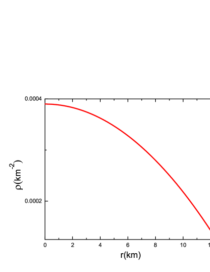
Figure 1: Variation of the energy-density, $\rho(r)$ within the stellar interior of the millisecond pulsar PSR J0514-4002A.

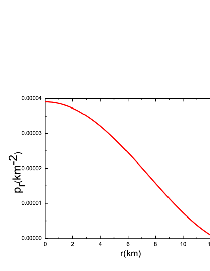
Figure 2: Variation of the radial pressure $p_{r}(r)$ within the stellar interior of the millisecond pulsar PSR J0514-4002A.

Figure 3: Variation of the transverse pressure $p_{t}(r)$ within the stellar interior of the millisecond pulsar PSR J0514-4002A.

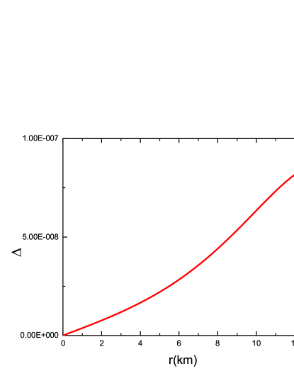
Figure 4: Variation of the anisotropic parameter, $\Delta$ within the stellar interior of the millisecond pulsar PSR J0514-4002A.

$\bf{Equation~{}of~{}State:}$

We know that different Equation of State (EoS) leads to different matter distribution of the pulsar and hence different Mass-Radius relation. Here, we have obtained a relation between density $(\rho)$ and radial pressure ($p_{r}$) which is known as Equation of State (EoS) by using curve fitting technique and interestingly it comes out to be polytropic in nature. The relation trace out given below:

$$p_{r}=\alpha\rho^{\beta}$$ (13)

where $\alpha$ is the polytropic constant and $\beta$ is related to polytropic index. As we know that $\beta=2$ implies for nonrelativistic degenerate fermions, whereas $\beta=1$ leads to stiff matter EoS. In our model, the numerical value of $\alpha$ and $\beta$ are comes out as $\alpha$=2.462$\times 10^{-7}$ and $\beta$=2.856 which indicates that the equation of state (EoS) of the pulsar is stiff(Fig. 5) ozel2006 ; Guo2014 ; Lai2009 .

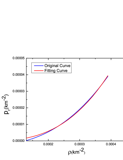
Figure 5: The equation of state (EoS) within the stellar interior of the millisecond pulsar PSR J0514-4002A.

3 Physical analysis

3.1 Exterior spacetime and matching condition

Our interior solution should match the exterior Schwarzschild metric at the boundary ($r=b$) where $b$ is the radius of the star. The exterior spacetime is given by the Schwarzschild line element

$$ds^{2}=-\left(1-\frac{2M}{r}\right)dt^{2}+\left(1-\frac{2M}{r}\right)^{-1}dr^{2}$$

$$+r^{2}(d\theta^{2}+sin^{2}\theta d\phi^{2})$$ (14)

Now at the boundary $r=b$ the coefficients of $g_{tt}$, $g_{rr}$ and $\frac{\partial g_{tt}}{\partial r}$ all are continuous. This implies

$$\left(1-\frac{b^{2}}{R^{2}}+4\frac{b^{4}}{A^{4}}\right) = 1-\frac{2M}{b},$$ (15)

$$B^{2}\sin^{2}\ln\sqrt{\frac{\sqrt{1-\frac{b^{2}}{R^{2}}+4\frac{b^{4}}{A^{4}}}+2\frac{b^{2}}{A^{2}}-\frac{1}{4}\frac{A^{2}}{R^{2}}}{C}}$$

$$=\left(1-\frac{2M}{b}\right)$$ (16)

and

$$\left(-\frac{2b}{R^{2}}+16\frac{b^{3}}{A^{4}}\right) = \frac{2M}{b^{2}}$$

Solving above equations we get,

$$R = \frac{b^{3/2}}{\sqrt{5M}}$$

$$A = \frac{\sqrt{2}b^{5/4}}{(3M)^{1/4}}$$

Furthermore, using the expression (12) for $p_{r}$(r=b)=0 we obtain

$$C = \frac{\sqrt{1-\frac{b^{2}}{R^{2}}+4\frac{b^{4}}{A^{4}}}+2\frac{b^{2}}{A^{2}}-\frac{1}{4}\frac{A^{2}}{R^{2}}}{e^{\delta}}$$

Where,

$$\delta = \left(2\cot^{-1}\{\frac{\frac{1}{b^{2}\left(1-\frac{b^{2}}{R^{2}}+4\frac{b^{4}}{A^{4}}\right)}-\frac{1}{b^{2}}}{2\frac{\left(1-\frac{b^{2}}{R^{2}}+4\frac{b^{4}}{A^{4}}\right)^{-1/2}\left(4\frac{b^{2}}{A^{4}}-\frac{1}{2R^{2}}\right)+\frac{2}{A^{2}}}{\left(\sqrt{1-\frac{b^{2}}{R^{2}}+4\frac{b^{4}}{A^{4}}}+2\frac{b^{2}}{A^{2}}-\frac{1}{4}\frac{A^{2}}{R^{2}}\right)}}\}\right)$$

Now from the equation  (15), we get the compactification factor as

$$u=\frac{M}{b}=\left(\frac{b^{2}}{2R^{2}}-2\frac{b^{4}}{A^{4}}\right).$$ (17)

3.2 Equilibrium analysis via generalized TOV-equation

To check whether our model is in equilibrium under three different forces($F_{g}$, $F_{h}$ and $F_{a}$), we consider the generalized Tolman-Oppenheimer-Volkov (TOV) equation which is represented by the formula

$$\frac{dp_{r}}{dr}+\frac{1}{2}\nu^{\prime}\left(\rho+p_{r}\right)+\frac{2}{r}\left(p_{r}-p_{t}\right)=0.$$ (18)

$$F_{h}+F_{g}+F_{a}=0,$$ (19)

where,

$$F_{h} = -\frac{dp_{r}}{dr}$$ (20)

$$F_{g} = -\frac{1}{2}\nu^{\prime}\left(\rho+p_{r}\right)$$ (21)

$$F_{a} = -\frac{2}{r}\left(p_{r}-p_{t}\right)$$ (22)

Generalized TOV(stellar) equation describes the system is in static equilibrium under gravitational ($F_{g}$), hydrostatic ($F_{h}$) and anisotropic ($F_{a}$) forces of the millisecond pulsar PSR J0514-4002A. The profiles of the above mention three forces of the pulsar are shown in Fig. 6. This figure shows that the gravitational force is counterbalanced by the hydrostatic force and anisotropic force, therefore consequently the present system hold in static equilibrium.

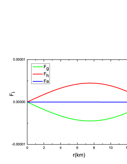
Figure 6: The behavior of gravitational ($F_{g}$), hydrostatic ($F_{h}$) and anisotropic ($F_{a}$) forces at the stellar interior of the millisecond pulsar PSR J0514-4002A.

3.3 Energy conditions verification

From the Fig. 7 we see that the following energy conditions like, null energy condition (NEC), weak energy condition (WEC), strong energy condition (SEC) and dominant energy condition (DEC) are satisfied in our model :
(i) NEC: $p_{r}+\rho\geq 0$ ,
(ii) WEC: $p_{r}+\rho\geq 0$ , $~{}~{}\rho\geq 0$ ,
(iii) SEC: $p_{r}+\rho\geq 0$ ,$~{}~{}~{}~{}3p_{r}+\rho\geq 0$ ,
(iv) DEC: $\rho>p_{r}$.

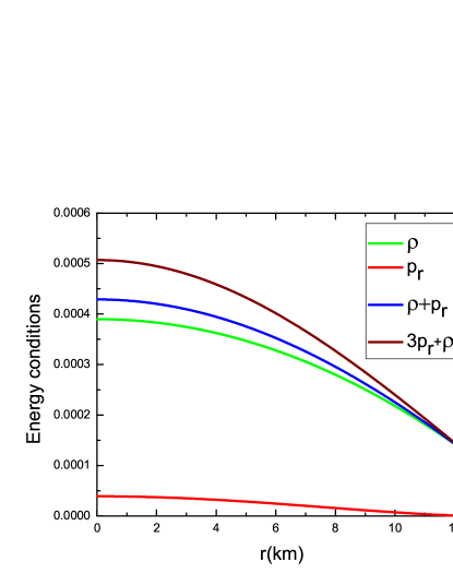
Figure 7: Energy conditions at the stellar interior of the millisecond pulsar PSR J0514-4002A.

3.4 Stability checking

Our proposed model for millisecond pulsar PSR J0514-4002A will be physically acceptable if the sound speed within the stellar interior is less than the speed of light (causality conditions), where the sound speed can be obtained as $v^{2}=\frac{dp}{d\rho}$Herrera1992 ; Abreu2007 . In our anisotropic pulsar model, we desire $v^{2}$ to be $0\leq v^{2}=(\frac{dp}{d\rho})\leq 1$. We plot the radial and transverse sound speed for the millisecond pulsar PSR J0514-4002A in Fig. 8 & Fig. 9 and observed that it satisfies well with the inequalities $0\leq v_{r}^{2}\leq 1$ and $0\leq v_{t}^{2}\leq 1$ everywhere within the pulsar. Therefore our pulsar model is well stable.

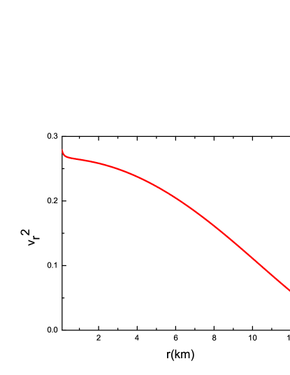
Figure 8: Variation of the radial sound speed ($v_{r}^{2}$) at the stellar interior of the millisecond pulsar PSR J0514-4002A.

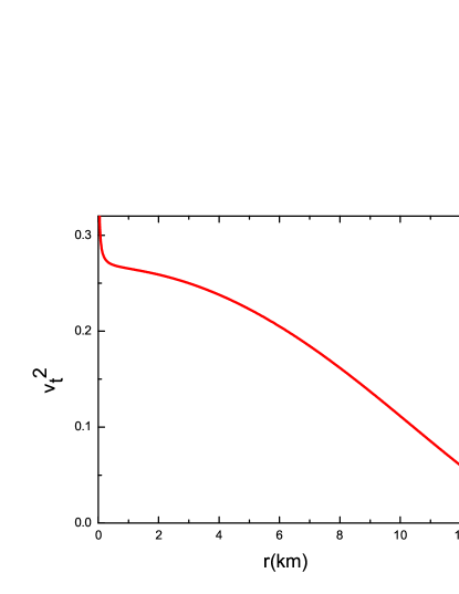
Figure 9: Variation of the transverse sound speed ($v_{t}^{2}$) at the stellar interior of the millisecond pulsar PSR J0514-4002A.

We also verify the dynamical stability in presence of thermal radiation. The adiabatic index($\gamma$) satisfies the condition $\gamma=\frac{\rho+p_{r}}{p_{r}}\frac{dp_{r}}{d\rho}>\frac{4}{3}$ everywhere within the pulsar (Fig. 10). This type of stability checking has previously done by several researcher Chandrasekhar1964 ; Bondi1964 ; Bardeen1966 ; Knutsen1988 ; Harko2013 .

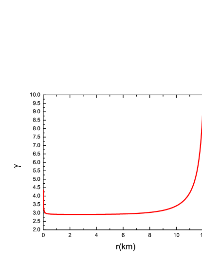
Figure 10: Adiabatic index ($\gamma$) at the stellar interior of the millisecond pulsar PSR J0514-4002A.

3.5 Compactness and Surface redshift

The mass function can be determined using the equation given below

$$M(r)=4\pi\int^{b}_{0}\rho~{}~{}r^{2}dr=\frac{b}{2}\left[\frac{b^{2}}{R^{2}}-4\frac{b^{4}}{A^{4}}\right]$$ (23)

where $b$ is the radius of the millisecond pulsar. According to Buchdahl Buchdahl1959 , for a spherically symmetric perfect fluid sphere, the allowable mass-radius ratio should be $\frac{Mass}{Radius}<\frac{4}{9}$.

The compactness, u is given by

$$u=\frac{M(b)}{b}=\frac{1}{2}\left[\frac{b^{2}}{R^{2}}-4\frac{b^{4}}{A^{4}}\right]$$ (24)

The surface red-shift ($Z_{s}$) corresponding to the above compactness ($u$) is

$$1+Z_{s}=\left[1-(2u)\right]^{-\frac{1}{2}},$$ (25)

where

$$Z_{s}=\frac{1}{\sqrt{1-\frac{b^{2}}{R^{2}}+4\frac{b^{4}}{A^{4}}}}-1$$ (26)

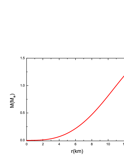
Figure 11: Mass function, M(r) at the stellar interior of the millisecond pulsar PSR J0514-4002A.

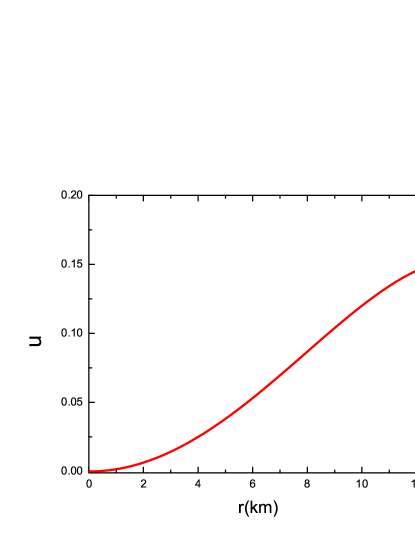
Figure 12: Compactness (u) at the stellar interior of the millisecond pulsar PSR J0514-4002A.

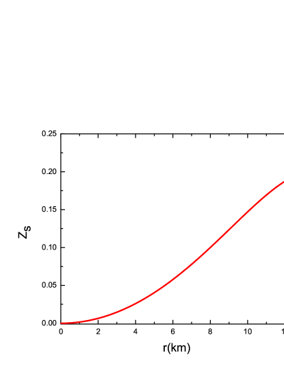
Figure 13: Surface red-shift ($Z_{s}$) against radial parameter r of the millisecond pulsar PSR J0514-4002A.

The variation of the mass function, compactness and surface red-shift of the millisecond pulsar PSR J0514-4002A are shown in Fig. 11, Fig. 12 and Fig. 13 respectively.

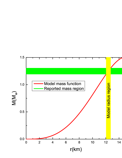
Figure 14: Possible radius of the MSP PSR J0514-4002A.

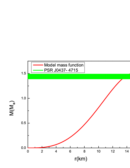
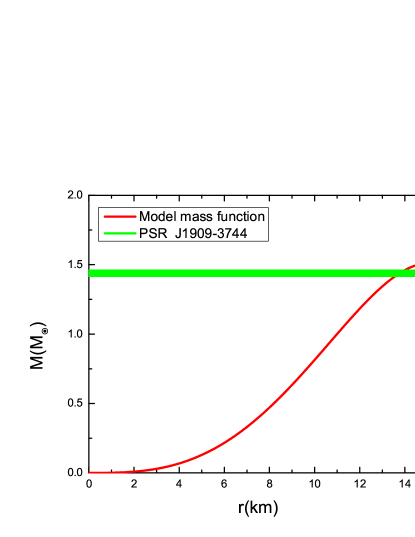
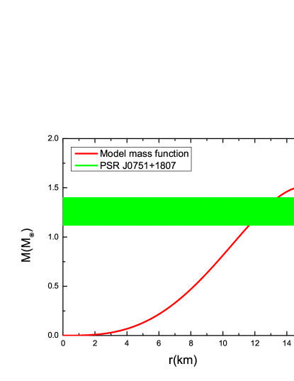
Figure 15: Application of our model for other millisecond Pulsars.

4 Discussion and concluding remarks

In this paper, we have investigated the nature of the newly discovered millisecond pulsar PSR J0514-4002A Ridolfi2019 by considering Tolman VII Tolman1939 metric and taking constituent matter as anisotropic in nature. Density and pressure of the newly discovered millisecond pulsar PSR J0514-4002A are well behaved (Figs. 1, 2, 3 and 4). Here, we have obtained a relation between density $(\rho)$ and radial pressure ($p_{r}$) which is known as Equation of State (EoS) by using curve fitting technique and interestingly it comes out as polytropic in nature. The relation trace out as $p_{r}=\alpha\rho^{\beta}$ where $\alpha$ is the polytropic constant and $\beta$ is related to polytropic index. The numerical value of $\alpha$ and $\beta$ are comes out as $\alpha$=2.462$\times 10^{-7}$ and $\beta$=2.856 which indicates that the equation of state (EoS) of the pulsar is stiff(Fig. 5) ozel2006 ; Guo2014 ; Lai2009 .

Our interior solutions has been matched to the exterior Schwarzschild line element at the boundary. Our model satisfies stellar equation (generalised TOV) and all energy conditions (Fig 6 and 7). It is stable according to Herrera stability condition Herrera1992 (Fig. 8 and 9). We have also check the dynamical stability of the model in presence of thermal radiation (Fig. 10). The mass function (M), compactness (u) and surface red-shift ($Z_{s}$) has been plotted in Fig. 11, Fig. 12 and Fig. 13 respectively. The constants R, A, C can be determined in terms of mass(M) and radius(b) by using the required physical boundary conditions. Taking into account, the mass $M_{p}=1.25^{+0.05}_{-0.06}M_{\odot}$ of the millisecond pulsar PSR J0514-4002A obtained by Ridolfi et al. Ridolfi2019 , we consider the values of the constants R = 17.5 km, A = 26.08 km and C = 0.06713, such that the pressure drops from its maximum value (at center) to zero at the boundary(Radius(b)= 12.39 km). As per our model, the possible radius of the millisecond pulsar PSR J0514-4002A has been found to be $12.39^{+0.31}_{-0.35}km$ (Fig. 14).

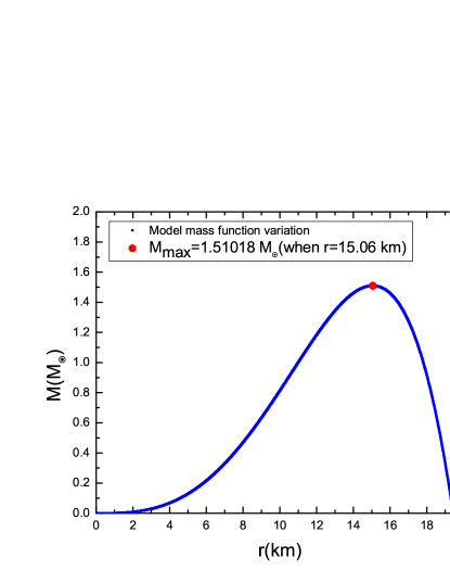
Figure 16: Mass function, M(r) at the stellar interior with a maximum mass $1.51M_{\odot}$.

The compactness ($u$) of the millisecond pulsar PSR J0514-4002A has been found to be 0.14875 which satisfies Buchdahl limit Buchdahl1959 . The surface red-shift ($Z_{s}$) for the millisecond pulsar PSR J0514-4002A has also found to be 0.193 which is $\leq$ 0.8, implies the validity of our model Haensel2000 ; Barraco2002 . It is to be mentioned here that while solving Einstein’s field equations, we set $c=G=1$. Now, inserting $G$ and $c$ into the relevant equations, the values of the central density and central pressure of our pulsar turn out to be $\rho_{0}$=0.52592$\times 10^{15}gm/cc$ (i.e. 0.000389767$km^{-2}$) and $p_{0}$=1.093$\times 10^{35}dyne/cm^{2}$ (i.e. 0.0000437354$km^{-2}$). It is worthy to be mention here that our pulsar model is well applicable to other millisecond Pulsars such as PSR J0437-4715, PSR J1909-3744, PSR J0751+1807 (Fig. 15). From Fig. 15, one can easily estimate the probable radii of these MSPs, once the radius is known with mass, other physical parameters can be calculated. More interestingly, our model can describe the characteristics of most of the pulsars having masses upto $1.51M_{\odot}$(Fig. 16).

Finally, we conclude by pointing out that our proposed model (having stiff EoS) not only can be used to study the physical properties of the millisecond pulsar PSR J0514-4002A, but also for other millisecond pulsars (like: PSR J0437-4715, PSR J1909-3744, PSR J0751+1807 etc.) having masses up to $1.51M_{\odot}$.

- (1) R. Cornelisse, M.M. Kotze, J. Casares, P.A. Charles, P.J. Hakala, MNRAS 436, 910 (2013)
- (2) M.A. Alpar, A.F. Cheng, M.A. Ruderman, J. Shaham, Nature 300, 728 (1982)
- (3) D.C. Backer, S.R. Kulkarni, C. Heiles, M.M. Davis, W.M. Goss, Nature 300, 615 (1982)
- (4) M. Ruderman, J. Shaham, M. Tavani, ApJ 336, 507 (1989)
- (5) W. Becker, J. Trmper, Nature 365, 528 (1993)
- (6) J. Antoniadis, T.M. Tauris, F. zel, E. Barr, D.J. Champion, P.C.C. Freire, preprint arXiv: 1605.01665 (2016)
- (7) A. Zilles, et al., MNRAS 492, 1579 (2020)
- (8) G. Voisin, et al., MNRAS 492, 1550 (2020)
- (9) N.V. Gusinskaia, et al., MNRAS 492, 1091 (2020)
- (10) M. Vivekanand, The Astrophysical Journal 890, 143 (2020)
- (11) S. Bogdanov, et al., The Astrophysical Journal Letters 887, L25 (2019)
- (12) T.E. Riley, et al., The Astrophysical Journal Letters 887, L21 ((2019)
- (13) P. Bult, et al., Astrophys. J. 885, L1 (2019)
- (14) N.A. Webb, et al., Astron. Astrophys. 627, A141 (2019)
- (15) C.M. Will, Living Rev. Rel. 9, 3 (2005)
- (16) K. Schwarzschild, Sitzer. Preuss. Akad. Wiss. 189, 424 (1916)
- (17) J.R. Oppenheimer, G.M. Volkoff, Phys. Rev. 55, 374 (1939)
- (18) R.C. Tolman, Phys. Rev. 55, 364 (1939)
- (19) F. Rahaman, et al., Gen. Relativ. Gravit. 44, 107 (2012)
- (20) F. Rahaman, et al., Eur. Phys. J. C 72, 2071 (2012)
- (21) M. Kalam, et al., Eur. Phys. J. C 72, 2248 (2012)
- (22) Sk.M. Hossein, et al, Int. J. Mod. Phys. D 21, 1250088 (2012)
- (23) M. Kalam, et al., Int. J. Theor. Phys. 52, 3319 (2013)
- (24) M. Kalam, et al., Eur. Phys. J. C 73, 2409 (2013)
- (25) M. Kalam, et al., Eur. Phys. J. C 74, 2971 (2014)
- (26) M. Kalam, et al., Astrophys. Space Sci. 349, 865 (2014)
- (27) Sk.M. Hossein, et al., Astrophys.Space Sci. 361,No.6, 203 (2016)
- (28) Sk.M. Hossein, et al., Astrophys.Space Sci. 361,No.10, 333 (2016)
- (29) M. Kalam, et al., Mod.Phys.Lett.A 31,No.40, 1650219 (2016)
- (30) M. Kalam, et al., Mod.Phys.Lett.A 32,No.04, 1750012 (2017)
- (31) M. Kalam, et al., Res.Astron.Astrophys. 18, No.3, 025 (2018)
- (32) S. Molla, et al., Res.Astron.Astrophys. 19, No.2, 026 (2019)
- (33) R. Islam, et al., Astrophys.Space Sci. 364,No.7, 112 (2019)
- (34) S.H.Hendi, et al., JCAP 09, 013 (2016)
- (35) S.H.Hendi, et al., JCAP 07, 004 (2017)
- (36) B. Eslam Panah, et al., Astrophys.J. 848,No. 1, 24 (2017)
- (37) S. Ngubelanga, S.D. Maharaj, S. Ray, Astrophys. Space Sci. 357, 74 (2015)
- (38) B.C. Paul, P.K. Chattopadhyay, S. Karmakar, Astrophys. Space Sci. 356, 327 (2015)
- (39) F. Lobo, Class. Quantum. Grav. 23, 1525 (2006)
- (40) K. Bronnikov, J.C. Fabris, Phys. Rev. Lett. 96, 251101 (2006)
- (41) E. Egeland, Compact Star, Trondheim, Norway (2007)
- (42) I. Dymnikova, Class. Quantum. Gravit. 19, 725 (2002)
- (43) N. Neary, M. Ishak, K. Lake, Phys. Rev. D 64, 084001 (2001)
- (44) T.E. Kiess, Astrophys. Space Sci. 339, 329 (2012)
- (45) A.M. Raghoonundun, D.W. Hobill, Phys. Rev. D 92, 124005 (2015)
- (46) P. Bhar, M.H. Murad, N. Pant, Astrophys Space Sci 359, 13 (2015)
- (47) K.N. Singh, F. Rahaman, N. Pant, Can. J. Phys. 94, 1017 (2016)
- (48) P. Bhar, K.N. Singh, N. Pant, Indian J Phys 91, 701 (2017)
- (49) H. Sotani, K.D. Kokkotas, Phys. Rev. D 97, 124034 (2018)
- (50) S. Hensh, Z. Stuchlík, Eur. Phys. J. C 79, 834 (2019)
- (51) A. Ridolfi, P.C.C. Freire, Y. Gupta, S.M. Ransom, MNRAS 490, 3860 (2019)
- (52) D.J. Reardon, et al., MNRAS 455, 1751 (2016)
- (53) B.A. Jacoby, A. Hotan, M. Bailes, S. Ord, S.R. Kulkarni, The Astrophysical Journal 629, L113 (2005)
- (54) D.J. Nice, et al., 2008, in 40 Years of Pulsars: Millisecond Pulsars, Magnetars and More, AIP Conf. Proc., 983, 453
- (55) M. Fortin, M. Bejger, P. Haensel, J.L. Zdunik, A&A 586, A109 (2016)
- (56) P.M. Takisa, S.D. Maharaj, L.L. Leeuw, Eur. Phys. J. C 79, 8 (2019)
- (57) D.K. Matondo, S.D. Maharaj, S. Ray, Eur. Phys. J. C 78, 437 (2018)
- (58) S.K. Maurya, Y.K. Gupta, S. Ray, S.R. Chowdhury, Eur. Phys. J. C 75, 389 (2015)
- (59) S.K. Maurya, A. Banerjee, M.K. Jasim, J. Kumar, A.K. Prasad, A. Pradhan, Phys. Rev. D 99, 044029 (2019)
- (60) B. Dayanandana, S.K. Maurya, T.T Smitha, Eur. Phys. J. A 53, 141 (2017)
- (61) S.K. Maurya, Eur. Phys. J. A 53, 89 (2017)
- (62) S. Gedela, R.K Bisht, N. Pant, Eur. Phys. J. A 54, 207 (2018)
- (63) K.N. Singh, N. Pant, M. Govender, Chinese Physics C 41, 015103 (2017)
- (64) M.A K Jafry, S. Molla, R. Islam, M. Kalam , Astrophys.Space Sci. 362,No.10, 188 (2017)
- (65) F. Rahaman, S.D. Maharaj, I.H. Sardar, K. Chakraborty, Mod. Phys. Lett. A 32, 1750053 (2017)
- (66) M.K. Jasim, S.K. Maurya, Y.K. Gupta, B. Dayanandan, Astrophys Space Sci 361, 352 (2016)
- (67) P.M. Takisa, S.D. Maharaj, Astrophys Space Sci 361, 262 (2016)
- (68) S.K. Maurya, M.K. Jasim, Y.K. Gupta, T.T. Smitha, Astrophys Space Sci 361, 163 (2016)
- (69) K.N. Singh, N. Pradhan, N. Pant, Pramana J. Phys. 89, 23 (2017)
- (70) F. zel, Nature 441, 1115 (2006)
- (71) Y.J. Guo, X.Y. Lai, R.X. Xu, Chinese Physics C 38, 055101 (2014)
- (72) X.Y. Lai, R.X. Xu, MNRAS 398, L31 (2009)
- (73) L. Herrera, Phys. Lett. A 165, 206 (1992)
- (74) H. Abreu, H. Hernandez, L.A Nunez, Class. Quantum. Grav. 24, 4631 (2007)
- (75) S. Chandrasekhar, Astrophys. J. 140, 417 (1964)
- (76) H. Bondi, Proc. R. Soc. Lond. A 281, 39 (1964)
- (77) J.M. Bardeen, K.S. Thorne, D.W. Meltzer, Astrophys. J. 145, 505 (1966)
- (78) H. Knutsen, MNRAS 232, 163 (1988)
- (79) M.K. Mak, T. Harko, Eur. Phys. J. C 73, 2585 (2013)
- (80) H.A. Buchdahl, Phys. Rev. 116, 1027 (1959)
- (81) P. Haensel, J.P. Lasopa, J.L. Zdunik, Nucl. Phys. Proc. Suppl. 80, 1110 (2000)
- (82) D. Barraco, V.H. Hamity, Physical Review D 65, 124028 (2002)