Chaos in the quantum Duffing oscillator in the semiclassical regime under parametrized dissipation

Abstract

We study the quantum dissipative Duffing oscillator across a range of system sizes and environmental couplings under varying semiclassical approximations. Using spatial (based on Kullback-Leibler distances between phase-space attractors) and temporal (Lyapunov exponent-based) complexity metrics, we isolate the effect of the environment on quantum-classical differences. Moreover, we quantify the system sizes where quantum dynamics cannot be simulated using semiclassical or noise-added classical approximations. Remarkably, we find that a parametrically invariant meta-attractor emerges at a specific length scale and noise-added classical models deviate strongly from quantum dynamics below this scale. Our findings also generalize the previous surprising result that classically regular orbits can have the greatest quantum-classical differences in the semiclassical regime. In particular, we show that the dynamical growth of quantum-classical differences is not determined by the degree of classical chaos.

I Introduction

Non-linearity is a quantum-mechanical resource useful in amplifying quantum-classical differences Jacobs and Landahl (2009). Quantum systems at the length and energy scales of current experimental relevance are best treated as open to the environment and are thus termed NISQ (noisy intermediate scale quantum) systems Preskill (2018). These environmental effects lead to decoherence but can also be exploited through measurement feedback Eastman et al. (2017); Shi et al. (2019). Experimentalists and theorists have both been interested in understanding the emergence of quantum behavior in such non-linear quantum dissipative systems (NQDS) Bakemeier et al. (2015); Li et al. (2012). Specifically, chaos, or sensitivity to initial conditions and parameters, in an NQDS is fundamentally different from Hamiltonian chaos Yusipov et al. (2019); Ghose et al. (2004); Kumari, Meenu (2019) and can be quantified using the Lyapunov exponent. In this context several groups including Pokharel et. al. Pokharel et al. (2018), Eastman et. al. Eastman et al. (2017), Yusipov et. al. Yusipov et al. (2019), Ralph et. al. Ralph et al. (2017) have shown that Lyapunov exponents for NQDS can have a smooth Ott et al. (1984); Dittrich and Graham (1987); Klappauf et al. (1998, 1999); Ammann et al. (1998); Pattanayak et al. (2003); Gong and Brumer (2005); Habib et al. (1998) but non-monotonic and rich quantum-to-classical transition. The details of the mechanism, including the role of the environment in this transition, have not been fully characterized.

In this context, we report on results from a study examining with care the effect of changing parameters on the complexity of the dynamics. We consider semiclassical approximations for the quantum Duffing oscillator that are derived from a quantum master equation under the assumption of a Markovian environment. In the process we find that visual correspondence between different phase-space Poincare sections does not translate to them having equal Lyapunov exponent and vice versa. Spatial and temporal complexity can be and are independent of each other (see Fig. 1). Therefore, we further analyze our semiclassical models using a Kullback-Liebler distance between phase space attractors as well as the corresponding Lyapunov exponents. Our results can be summarized as follows:

• The primary effect of decreasing length scales is seen to be the increasing sensitivity to environmental fluctuations for systems of smaller size. However, this behavior is not explained by the effects of adding Gaussian noise to the classical system. Artificial noise-added classical systems reproduce some of the qualitative behavior of quantum noise temporally, but are measurably spatially different.

• At a certain length-scale the environment washes out difference between classically chaotic and periodic trajectories. Consequently, a chaotic meta-attractor emerges which is invariant to changes in environmental coupling. For systems that are smaller than this length-scale, noise-added classical models diverge significantly from the semiclassical dynamics.

• The deviation from the classical limit is maximal for those systems where the global attractor is a classical periodic orbit (PO). In other words, in keeping with previous results Pokharel et al. (2018) these POs are more sensitive to environmental effects of changing length scales than classically chaotic orbits and quantum-classical correspondence requires larger length-scales for POs than for chaos.

• In contrast to the standard intuition, even for chaotic systems the degree of classical chaos i.e. the maximal classical Lyapunov exponent is not correlated to the length-scale where the classical and semiclassical dynamics deviate.

Thus, the careful consideration of Lyapunov exponents and the use of other measures reveal that the quantum to classical transition for NQDS is filled with a wealth of non-intuitive phenomena arising from the interplay between chaos, noise and quantum-effects at this scale. In what follows, we present our basic models and methods, before turning to results and a concluding discussion.

II Methods

The Duffing oscillator is a paradigmatic model to study quantum to classical transition for chaos. The Newtonian model consists of a unit mass in a double-well potential with dissipation $\Gamma$, sinusoidal driving amplitude $g$, frequency $\omega$, and dimensionless length scale $\beta$,

$$\ddot{x}+2\Gamma\dot{x}+\beta^{2}x^{3}-x=\frac{g}{\beta}cos(\Omega t).$$ (1)

The quantum Duffing oscillator is described using Quantum State Diffusion theory Percival (1998) where the stochastic evolution of a single pure quantum system $|\psi\rangle$ under continuous measurement (including by the environment, for example) is considered. For this open system evolution, the Hamiltonian is

$$\hat{H}=\frac{1}{2}\hat{P}^{2}+\frac{\beta^{2}}{4}\hat{Q}^{4}-\frac{1}{2}\hat{Q}^{2}+\frac{\Gamma}{2}(\hat{Q}\hat{P}+\hat{P}\hat{Q})-\frac{g}{\beta}\hat{Q}\cos(\Omega t),$$ (2)

and dissipation due to coupling to the environment is represented by a single Lindblad operator $\hat{L}=\sqrt{\Gamma}(\hat{X}+i\hat{P})$ Brun et al. (1996). The corresponding Langevin-Ito equation for the evolution of the wavefunction is then

$$\begin{split}|d\psi\rangle&=-\frac{i}{\hbar}\hat{H}|\psi\rangle dt+\sum_{j}(\hat{L_{j}}-\langle\hat{L_{j}}\rangle)|\psi\rangle d\xi_{j}+\sum_{j}(\langle\hat{L}^{\dagger}_{j}\rangle\hat{L}_{j}\\ &-\frac{1}{2}\hat{L}^{\dagger}_{j}\hat{L}_{j}-\frac{1}{2}\langle\hat{L}^{\dagger}_{j}\rangle\langle\hat{L}_{j}\rangle)|\psi\rangle dt.\end{split}$$ (3)

In this system, both the dissipation and the quantum non-linearity scale with $\Gamma$, via $\hat{L}$. The stochastic nature of the dynamics arises from independent normalized complex differential random variables $d\xi_{j}$, where the mean over realizations $M$ satisfies $M(d\xi_{j})=0\ ,M(d\xi_{j}d\xi^{\prime}_{j})=0\ ,M(d\xi_{j}d\xi^{\prime*}_{j})=\delta_{j\prime j}dt$.

This formulation of the Duffing oscillator has a single parameter $\beta\equiv\sqrt{\frac{\hbar}{l^{2}m\omega_{0}}}$ that determines the scale the system. The dynamics of Eq. 1, defines the ‘classical limit’, which is invariant under change in $\beta$ except for change of the length-scale. However, the dynamics of Eq. 3 do vary with $\beta$; in particular Eq. 1 can be derived for the expectation values of the position $\hat{X},\hat{P}$ for the evolving $|\psi\rangle$ as $\beta\rightarrow 0$. Thus, this parameter allows us to study the transition from the quantum scale $\beta\rightarrow 1$ to $\beta\to 0$, the largest length scales where the quantum predictions become scale invariant and agree identically with the Newtonian predictions. In other words, $\beta$ represent the level of ‘quantumness’ of the system. For our investigation, we focus on non-trivial damping $0<\Gamma<0.35$ with $g=0.3$, $\Omega=1$ as in Pokharel et al. (2018), with an interval of $\delta\Gamma=0.002$.

Previous work including that of Pokharel et al. Pokharel et al. (2018) used a semiclassical stochastic equation under the assumption that the wave function is sufficiently sharply localized by the action of the environment. In particular, this description reduces the dynamics to that of the first and second order moments of the position and the momentum, $x=\langle\hat{X}\rangle,p=\langle\hat{P}\rangle,\mu=\sigma_{XX},\kappa=\sigma_{PP},R=\frac{1}{2}(\sigma_{XP}+\sigma_{PX})$ where $\sigma_{AB}=\langle(A^{\dagger}-\langle A\rangle^{*})(B-\langle B\rangle)\rangle$. It is possible to reduce this system further – decreasing the number of variables in this stochastic ODE from five to four (see Appendix A) – by observing a conserved quantity $\mu\kappa-R^{2}=\frac{1}{4}$ and making a change of variables $\mu=\rho^{2},R=\rho\Pi$. This yields the following semiclassical equations for the Duffing oscillator:

$$dx=pdt+2\sqrt{\Gamma}\bigg{(}\bigg{(}\rho^{2}-\frac{1}{2}\bigg{)}d\xi_{R}-\rho\Pi d\xi_{I}\bigg{)},$$ (4)

$$\begin{split}dp&=\bigg{(}-\beta^{2}x^{3}+(1-3\beta^{2}\rho^{2})x-2\Gamma p+\frac{g}{\beta}\cos(\omega t)\bigg{)}dt\\ &+2\sqrt{\Gamma}\bigg{(}\rho\Pi d\xi_{R}-\bigg{(}\frac{1}{2}-\Pi^{2}-\frac{1}{4\rho^{2}}\bigg{)}d\xi_{I}\bigg{)},\end{split}$$ (5)

$$\frac{d\rho}{dt}=\Pi+\Gamma\bigg{(}\rho-\rho^{3}-\rho\Pi^{2}+\frac{1}{4\rho}\bigg{)},$$ (6)

$$\frac{d\Pi}{dt}=\rho(-3\beta^{2}x^{2}+1)+\frac{1}{4\rho^{3}}-\Gamma\Pi\bigg{(}1+\Pi^{2}+\rho^{2}+\frac{3}{4\rho^{2}}\bigg{)}.$$ (7)

This system can be understood as the $x,p$ oscillator coupled to the $\rho$, $\Pi$ oscillator, with the latter two variables representing the spread variables. The classical system is recovered from the semiclassical approximation by increasing the system size i.e. by letting $\beta\rightarrow 0$. The semiclassical model shows quantum features in three ways: 1) the influence of the spread variables $\rho$ and $\Pi$, 2) the environmental coupling appearing via noise terms proportional to $2\sqrt{\Gamma}$ for $dx$ and $dp$, and 3) a tunneling-like effect where the size of the barrier between the two wells of the oscillator is proportional to $(1-3\beta^{2}\rho^{2})$. In fact, this model can be described using a two-dimensional oscillator with the potential Shi et al. (2019)

$$\begin{split}U(x,\rho)=-(1-3\beta^{2}\rho^{2})\frac{x^{2}}{2}+\beta^{2}(\frac{x^{2}}{2})^{2}-(\frac{g}{\beta}\cos\omega t)x-\frac{\rho^{2}}{2}+\frac{1}{8\rho^{2}}\end{split}$$ (8)

that is also subject to noise and dissipation. In the remainder of the paper, we refer to this semiclassical model as “SC.”

Recall that Eq. (1) is $\beta$ invariant other than a change in the length scales. Therefore, the natural scale of analysis is $x\beta,p\beta$. Under these ‘scaled’ coordinates, the stochastic term in the semiclassical Eqns. (4,5) scale with $\beta$, while the tunneling term $1-3\beta^{2}\rho^{2}$ scales with $\beta^{2}$. It is therefore likely that the initial effect of increasing $\beta$ away from the classical limit arises from the stochastic terms. To isolate the effect of noise, we create a third model based on SC by fixing $\beta=10^{-5}$ – a nearly classical length-scale where the semiclassical dynamics overlaps with Newtonian dynamics – and allowing for a scaling of the noise terms by a factor $\beta_{n}$ so that $d\xi_{R,I}\rightarrow\beta_{n}d\xi_{R,I}$. We refer to this complex-noise added classical model as “$\text{C}+\mathcal{N}_{\mathbb{C}}$”. If our hypothesis about the role of the environment is correct, varying $\beta_{n}$ for $\text{C}+\mathcal{N}_{\mathbb{C}}$ should reproduce the effect of varying $\beta$ for SC. This immediately raises the question of whether a Gaussian noise-added classical model can reproduce the semiclassical dynamics without having to go through the semiclassical dynamics. To this end we consider the Duffing oscillator with a noise term $2\sqrt{\Gamma}d\xi$ added to the classical Duffing equations, resulting in

$$dx=pdt+2\sqrt{\Gamma}d\xi$$ (9)

$$dp=-\beta^{2}x^{3}+x-2\Gamma p+\frac{g}{\beta}\cos(\omega t)dt+2\sqrt{\Gamma}d\xi.$$ (10)

This real-noise added model is referred to as $\text{C}+\mathcal{N}_{\mathbb{R}}$.

Having established our various models to study the quantum-classical transition, we now turn to the quantitative metrics used to characterize how the dynamics change as a function of system size. For example, the standard tool for characterizing complex dynamics via measuring sensitivity to initial conditions is the largest Lyapunov exponent ($\lambda$) which distinguishes chaotic ($\lambda>0$) and periodic ($\lambda\leq 0$) dynamics Boffetta et al. (2002). We calculate $\lambda$ using the canonical methods Wolf et al. (1985). However, since the Lyapunov exponent of POs for the classical Duffing oscillator at a given $\Gamma$ is $\lambda_{\text{PO}}=-\Gamma$, we also use the previously introduced Pokharel et al. (2018) dynamical complexity $K=\lambda+\Gamma$ to quantify how much more complex a given orbit is compared to the minimum case of a PO. $K$ is strictly non-negative and compensates for the natural phase-space volume shrinkage caused by increasing dissipation $\Gamma$ (see Fig. 2). As a result, here $K$ allows for an effectively binary classification of Duffing attractors (see Fig. 2) across $\beta$ and $\Gamma$ with complex chaotic attractors having $0.2<K<0.3$ and simple periodic attractors having $K<0.2$, independent of $\Gamma$.

Despite their widespread and standard use, Lyapunov exponents can miss nuances in the underlying dynamics. In particular, the Lyapunov exponent quantifies the average temporal complexity and not the spatial complexity. The standard side-by-side comparison of Poincare sections, in this case for different semiclassical approximations (as shown in Fig. 1), can be somewhat informative in understanding spatial complexity differences. However, different stochastic terms (Eqs. 4, 5, 6 and 7) “blur” the Poincare sections in different ways that are not visually distinguishable. In other words, visual comparisons do not allow us to quantify the differences between dissimilar Poincare sections or to rank-order dissimilarity. To this end, we introduce a Kullback-Leibler inspired spatial similarity metric $d$ that allows us to compare different phase-space Poincare sections. In particular, for two histogram distributions $f_{1}(x)$ and $f_{2}(x)$, the distance $l$ Pattanayak et al. (2003) is defined as

$$l(f_{1},f_{2})=-\ln\left[\frac{\int\Big{(}f_{1}(x)\cdot f_{2}(x)\Big{)}^{2}\mathrm{d}x}{\Big{(}\int f_{1}(x)\cdot f_{1}(x)\mathrm{d}x\Big{)}\Big{(}\int f_{2}(x)\cdot f_{2}(x)\mathrm{d}x\Big{)}}\right].$$ (11)

Given a dynamical model $M$ (semi-classical or noise-added classical), we compute the $l$ over each coordinate of the phase space and take the Eulerian sum

$$d_{M_{1},M_{2}}(\Gamma_{1},\beta_{1};\Gamma_{2},\beta_{2})=\sqrt{\sum\limits_{j\in\{x,p\}}l\left(M_{1}^{j}(\Gamma_{1},\beta_{1}),M_{2}^{j}(\Gamma_{2},\beta_{2})\right)^{2}}$$ (12)

where $M^{j}$ is the coarse-grained Poincare-section histogram for the $j$-th phase-space coordinate. Note that we do not consider the coordinates $\rho,\Pi$ as they are only defined for SC and $\text{C}+\mathcal{N}_{\mathbb{C}}$. Two identical Poincare sections yield $d=0$ and two orthogonal sections yield $d\rightarrow\infty$. This distance is only well-defined for chaotic trajectories; for periodic trajectories, the distributions are too localized and even slight differences can lead to large distances (see Appendix B for more details).

III Results and Discussion

Figure 1: Different approximations are compared to the semiclassical model. Chaotic attractors for the Duffing oscillator at a representative environmental coupling ($\Gamma=0.174$) and system size ($\beta=\beta_{\text{conv}}$) are shown. The four figures are obtained under different semiclassical approximations described in more detail in the text. Note that while (c) and (d) are hard to distinguish visually, they are well-separated using the Lyapunov exponent or the SKL measure. At the same time, attractors in (a) and (c), and (b) and (d) have the same Lyapunov exponent respectively. All four approximations have a unique distance $d$ from SC, with cruder approximations appropriately having a larger $d$.

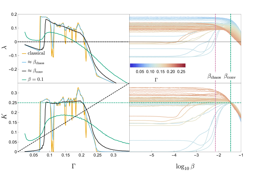
Figure 2: The Lyapunov exponent ($\lambda$) and the dynamical complexity ($K$) as a function of dissipation $\Gamma$ and system size $\beta$ are shown. The right two plots focus on $0.088<\Gamma\leq 0.2$. Both plots show that all classically periodic orbits become chaotic at $\beta=\beta_{\text{chaos}}$. Classically chaotic dynamics, in comparison, are robust as the length scales decreases. Note also that there is a convergence of the dynamical complexity at $\beta_{\text{conv}}$. This convergence is also confirmed using $d$ in Fig. 4.

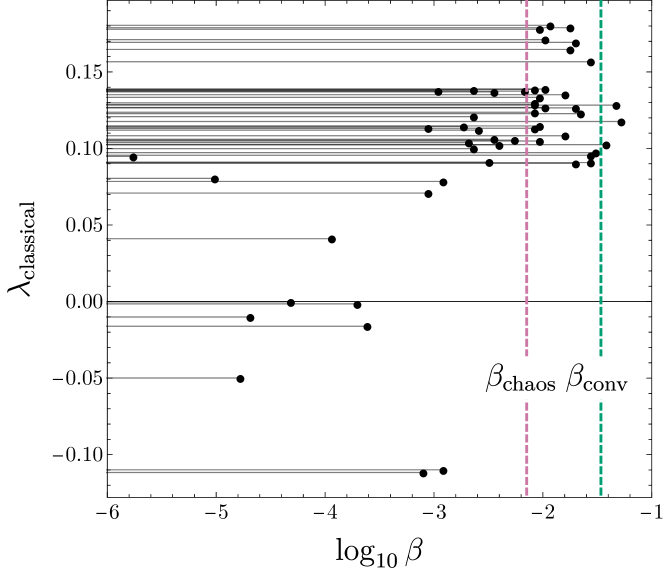
Figure 3: $\beta_{\text{break}}$ is the length scale at which $\lambda(\beta)$ diverges from the classical Lyapunov. $\beta_{\text{break}}$ as a function of $\lambda_{\text{classical}}$ is shown.

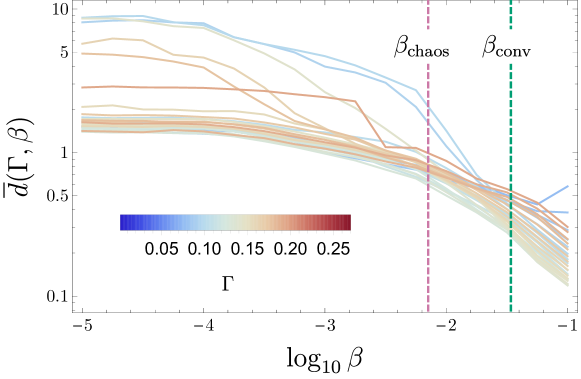
Figure 4: The mean distance between a given oscillators at some $\Gamma$ and all its counterparts in the range $[0.088,0.2]$ is shown. Corroborating the observation in Fig. 2, this distance between all attractors is decreasing for all oscillators, with all attractors becoming indistinguishable from the meta-attractor as the length-scale decreases.

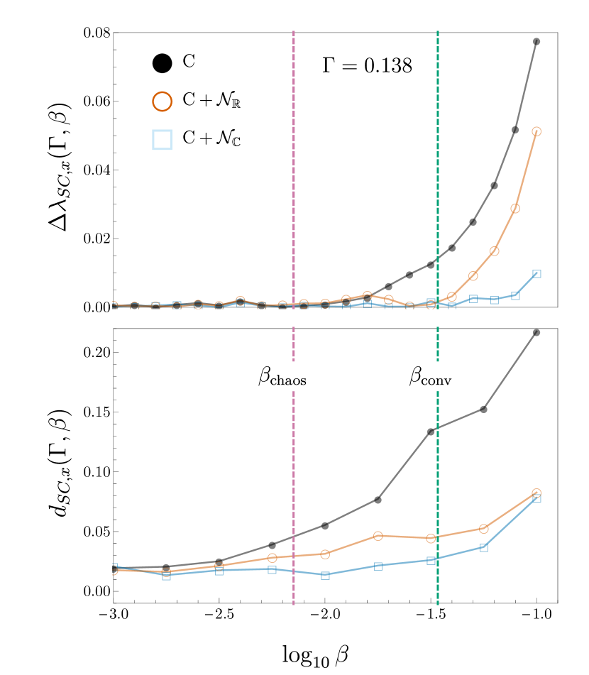
Figure 5: The change in difference between semiclassical approximations as a function of system size as captured by $\Delta\lambda$ and $d$. The oscillator chosen is the central oscillator, which has $\Gamma=0.138$. For this $\Gamma$ both metrics show a monotonic increase in the difference as the system size gets smaller and quantum effects become more prominent. However, the difference in dynamics at a larger system sizes is visible in $d$, than in $\lambda$. In other words, there exist length scales (for instance $\beta=\beta_{\text{chaos}}$) for which approximate models do not reproduce the spatial attractor, even though the Lyapunov exponent is reproduced.

Figure 6: $\Delta\lambda$ and $d$ shown as a function of length scale $\beta$, while averaged over various $\Gamma$ ranges. Even though different approximations to the semiclassical are visually (in terms of Poincare sections) and qualitatively similar to the full semiclasssical model, the difference between the models can quantified. Just like Fig. 5, both difference measures are monotonic in (a) and (d) for classically chaotic attractors, other than an anomalous peak at $\log_{10}\beta=-2.75$ (see Appendix for more details). On the other hand, classically periodic orbits are the hardest to recover using approximate semiclassics: the non-monotonic behavior of $\Delta\lambda$ over the entire range of $\Gamma$ is due to the classically periodic orbits in (b) and (e).$\Delta\lambda$ and $d$ between the semiclassical and noise-added classical models is the highest at $\beta=\beta_{\text{chaos}}$, after which all oscillators become chaotic. At $\beta=\beta_{\text{conv}}$, noise washes out the differences between different oscillators leading to the convergence shown in Fig2and3; and all the approximate semiclassical models lose relevance for $\beta<\beta_{\text{conv}}$.

At the classical limit, the Duffing oscillator has a standard bifurcation transition between regularity and complexity as a function of most dynamical parameters. Changing the strength $\Gamma$ of the coupling to the environment (which classically affects only the dissipation due to the environment and not fluctuations) also induces this behavior, including windows of periodic behavior and a regime of co-existing attractors. This parametric sensitivity which leads to abrupt changes in dynamical behavior has potential consequences in metrology as well applications in quantum control Eastman et al. (2017). Before we proceed to map the details of how the variety of classical dynamics and the classical sensitivity to parameters behave under change of length scale, we first establish the value of independently analyzing temporal complexity (using $\lambda$) and spatial similarity (using $d$). To do this, consider a classically chaotic attractor at $\Gamma=0.174$ under different approximations $\text{C},\text{C}+\mathcal{N}_{\mathbb{R}}\text{, and }\text{C}+\mathcal{N}_{\mathbb{C}}$. In Fig. 1 we compute $\lambda$ and the distance $d_{SC,x}$ for different semiclassical approximations. We find that:

• phase-space attractors that look different (like Fig. 1(b) and 1(d)) are quantifiably more similar to each other in $d$ than ones that at first appearance look similar (Fig. 1(a) and 1(d)).

• statistical differences between the semiclassical (SC) and classical-noise added model ($\text{C}+\mathcal{N}_{\mathbb{R}}$), which is missed by $\lambda$, do produce quantitatively and visually different spatial complex Poincare sections (Fig. 1(b) and 1(d)),

• even though the phase-space attractors for $\text{C}+\mathcal{N}_{\mathbb{C}}$ and SC are visually nearly identical, there are differences that can be captured by using $d$ (Fig. 1(c) and 1(d)),

With these caveats in mind, consider the temporal complexities $\lambda(\Gamma)$ and $K(\Gamma)$. The $\Gamma$ landscape can be divided classically into three regimes: low ($\Gamma<0.068$), intermediate ($0.068\leq\Gamma<0.2$) and high ($\Gamma>0.2$). In the low-damping regime, the orbits are regular orbits that traverse both wells of the Duffing oscillator; while in the high-damping regime, owing to the overwhelming magnitude of $\Gamma$ we observe single-well regular orbits.

Motivated by the inherent linearity of Hamiltonian quantum dynamics, it has been suggested that quantum mechanics makes systems more regular. Further, as a result, the quantum-classical difference are argued to scale with the Lyapunov exponent of the classical dynamics, with the classically chaotic systems having maximal deviation from quantum behavior. However, in NQDS in general and Fig. 2 in particular, we see all four possible transitions as a function of $\beta$: regular-to-regular, regular-to-chaos, chaos-to-regular and chaos-to-chaos. For example, the lower portion of the intermediate regime ($0.068\leq\Gamma<0.088$) shows a transition from classical chaos to semiclassical regularity. Here quantum effects delay the impact of increasing dissipation. Therefore, we see a ‘quantum regularization’ of chaos and the increase in $\lambda$ as a function of $\Gamma$ gets shifted. Some of the interesting effects due to the existence of a co-existing attractor in this regime are discussed further in Appendix E. The bulk of our analysis here, however, focuses on the intermediate regime $0.088\leq\Gamma<0.2$. Here we see chaos-to-chaos and regular-to-chaos transitions as a function of $\beta$.

To further clarify the effect of decreasing effective system action consider the behavior of temporal complexity as function of $\beta$ in Figs. 2 and 3. As Pokharel et. al. Pokharel et al. (2018) previously noted, introducing more quantum effects (increasing $\beta$) decreases the parametric sensitivity of temporal complexities to $\Gamma$ when compared to the classical system. This ‘chaotificiation’ is evident in the smoothing of the jaggedness of $K(\Gamma)$ (where the jaggedness corresponds to dips of regularity arising from higher order POs) as we scan $\beta>\beta_{\text{classical}}$. This can be understood as arising primarily because the addition of ‘quantum’ terms to the classical equations quickly destroys the higher period POs, which rely on dynamical synchronization across many periods. Consequently, all periodic attractors for $\Gamma\in(0.088,0.2]$ become chaotic for scales below $\beta_{\text{chaos}}=0.0068$. Moreover, the temporal complexity curves $\lambda(\beta),K(\beta)$ are highly non-monotonic and idiosyncratic as a function of $\beta$ (see Fig. 2). This is clearly a distinctive feature of NQDS.

A re-plotting of temporal complexity with a focus at the length scales where the classical dynamics no longer agrees with the semiclassical dynamics (i.e. $\beta_{\text{break}}$) is shown in Fig. 3. Here not only is $\beta_{\text{break}}$ lower for classical POs but also the break-scale is not intuitively related to the degree of chaos in the classical system $\lambda_{\text{classical}}$. This is in contrast to the standard arguments about quantum ‘break time’ that have persisted in the literature for many decades Berman and Zaslavsky (1978) but were constructed without considering the fact that genuine quantum-classical correspondence is only obtained by considering the effect of decoherence via the environment.

Further, while $\lambda$ and $K$ both capture $\beta$-invariance, only $K$ captures that the complexity of the dynamics becomes invariant of environmental coupling $\Gamma$ at a certain length scale. To be more specific, at a particular degree of quantumness $\beta=\beta_{\text{conv}}=0.0341$, $K(\Gamma)$ flattens. This remarkable convergence in dynamical complexity is verified by looking at the spatial similarity between the phase-space attractors. In particular, in Fig. 4, we compute the average distance between a trajectory at $\Gamma$ to all its counterparts in the range $\Gamma\in(0.088,0.2]$ under the same model $M$ and system size $\beta$

$$\overline{d}(\Gamma,\beta)=\text{mean}_{\Gamma^{\prime}}d_{M,M}(\Gamma,\beta;\Gamma^{\prime},\beta).$$ (13)

This average spatial similarity between attractors decreases as a function of system size. In other words, near $\beta_{\text{conv}}$ both spatial and temporal complexity are invariant under changes in the environmental coupling.

To summarize, the competition between environmental effects and chaos is richest in between $\beta_{\text{classical}}\leq\beta\leq\beta_{\text{conv}}$, the upper and lower boundaries of which have $\beta$ and $\Gamma$ invariant attractors respectively. As we detail below, $\text{C}+\mathcal{N}_{\mathbb{C}}$ closely mirrors semiclassical dynamics for systems larger than $\beta_{\text{conv}}$, which means that this range of scales is where noise from environmental coupling plays a significant role. At the same time, other than qualitative differences in how classically chaotic and regular orbits behave as a function of system size, there is no clear connection between the degree of classical chaos and quantum-classical deviation.

Now we turn from individual behavior to global characterization of various models. To do this, we compare the dynamics under different models by averaging distances over different parameters. In particular, we define a measure of the distance between two different models $M_{1}$ and $M_{2}$ at some specified system size $\beta$ and averaged over a range of $\Gamma$ as:

$$\overline{d}_{M_{1},M_{2}}(\beta)=\text{mean}_{\Gamma}\ d_{M_{1},M_{2}}(\Gamma,\beta;\Gamma,\beta).$$ (14)

An equivalent similarity metric can also be defined for comparing temporal complexity

$$\overline{\Delta\lambda}_{M_{1},M_{2}}(\beta)=\text{mean}_{\Gamma}\left|\lambda_{M_{1}}(\Gamma,\beta)-\lambda_{M_{2}}(\Gamma,\beta)\right|.$$ (15)

We start with a typical case of a classically chaotic attractor at $\Gamma=0.138$ in Fig. 5. Here we see that: a) all of the approximations to the accurate semiclassics get monotonically worse as the system size decreases; b) as we increase the number of semiclassical terms, the difference between the noise-added models and the semiclassical model decreases i.e. that $\text{C}+\mathcal{N}_{\mathbb{C}}$ does better than $\text{C}+\mathcal{N}_{\mathbb{R}}$; c) comparing the top and the bottom figures, we notice that even when the Lyapunov exponents under different models are identical, for instance at $\beta_{\text{chaos}}$, the underlying attractors might not be spatially similar. As we discuss below, b) and c) remain true in general for both classically chaotic and regular oscillators, but a) need not.

This simplicity does not persist in the aggregate behavior shown in Fig. 6. Here the figures in third column are averaged over all $\Gamma$ in the range $(0.088,0.2]$ and are the weighted sum of the first two columns, which are over the classically chaotic and periodic trajectories respectively. The aggregate behavior looks far more structured and to understand this structure, we first note that the rapid fluctuation in $\overline{\Delta\lambda}(\beta)$ for $\text{C}+\mathcal{N}_{\mathbb{C}}$ are of the order $10^{-3}$ which are inherent numerical precision errors arising from how the Lyapunov exponents are computed and further visually amplified by the log-scale. Apart from the overall increasing deviation of noise-added models from the semiclassical model SC as a function of $\beta$, there are several non-monotonic features which we now discuss.

The non-monotonicity of $\overline{\Delta\lambda}(\beta)$ for the overall average behavior in Fig. 6(c) is due to the classical POs, as clearly seen in Fig. 6(b). The peak of $\Delta\lambda$ near $\beta_{\text{chaos}}$ in Fig. 6(b) highlights the sensitivity of classical POs to Gaussian noise as this sensitivity drops when all trajectories are chaotic for $\beta>\beta_{\text{chaos}}$. Put differently, the semiclassical behavior of classical POs is harder to estimate using classical-noise added models and consequently requires the more sophisticated dynamical description given by $\text{C}+\mathcal{N}_{\mathbb{C}}$ and SC.

The non-monotonicity in $\overline{d}(\beta)$ is largely due to an anomalous peak at $\log_{10}\beta=-2.75$, most visible in Fig. 6(d) and 6(f). At this $\beta$-value, we see a single-well chaotic attractor in the noise-added models, which is spatially different from the true semiclassical double-well attractor (see Appendix B for more details). This peak in $\overline{d}(\beta)$ is not picked up by the Lyapunov exponents. Overall, we find that the spatial metric measuring the difference between phase-space attractors, $d$, does better at distinguishing between different models than $\lambda$. This emphasizes the need to use both spatial and temporal complexity metrics separately to study NQDS. Even when averaged, we see that spatial and temporal similarity of the models to the semiclassical dynamics gets progressively better as we use more sophisticated approximations. Moreover, for $\beta<\beta_{\text{conv}}$ the $\text{C}+\mathcal{N}_{\mathbb{C}}$ model approximates the semiclassical model well. This close similarity between SC and $\text{C}+\mathcal{N}_{\mathbb{C}}$ suggests that increased sensitivity to the environment is the dominant mechanism by which quantum effects manifest in this NQDS.

IV Conclusion

Nonlinear quantum dissipative systems evolve under an interplay between quantum effects, noise, and non-linearity. Our exploration of the quantum-classical transition in an NQDS, in particular a noisy nonlinear driven oscillator, shows that the semiclassical regime of NQDS remains an intriguing regime for further exploration. We demonstrate that while Lyapunov exponents and visual examinations of the phase space Poincare sections provide a reasonable first gauge of change in dynamical complexity or attractor similarity across systems, more careful metrics provide a better and more nuanced insights about this transition. We have also investigated whether the semiclassical dynamics here can be explained by simply adding classical noise. We find that while classical noise produces certain qualitative features, there are spatial and temporal quantitative features that require taking quantum effects into account. Surprisingly, the length scale for the breakdown of classical approximations to quantum behavior is not determined by the degree of classical chaos in the system, and the growth of quantum-classical difference is in general quite idiosyncratic. Such semiclassical techniques have been studied and used widely over the decades, particularly in chemical physics  Prezhdo (2002); Tomsovic and Heller (1991); Banerjee et al. (2004). Therefore, understanding what precisely does determine the break length scale is of great interest and remains an interesting avenue for further work. Further, we find that smaller systems that are more ‘quantum’ have few complicated periodic orbits due to increased sensitivity to environmental fluctuations. They are thus less sensitive to parameter variation than their classical counterparts. Remarkably, this leads to a chaotic meta-attractor fairly deep in the quantum regime that exhibits dynamical complexity relatively independent of the length-scale or environmental coupling. Arguably, even our most sophisticated semiclassical model, which implicitly uses an environment consisting of a Markovian bath at zero temperature, remains relatively simple. In particular, considering a finite bath at a finite temperature with manifestly non-Markovian features would allow for richer investigation of NQDS. Analyzing how features of the current analysis are altered by different, more sophisticated noise spectra, is another obvious next challenge.

V Acknowledgments

We would like to thank Bruce Duffy for computational support, and BP would like to thank Namit Anand for insightful discussions. AP is grateful for HHMI funding through Carleton, and internal funding from Carleton for student research.

Appendix A Derivation of the four equation semiclassical model

The dissipative dynamics of the open semiclassical Duffing oscillator results in a conserved quantity, corresponding to reducing the wavefunction to one which is a minimum uncertainty wavepacket. This enables the five equation semiclassical Duffing oscillator model from Pokharel et al. (2018) to be reduced to four equations. To be more explicit,

$$dx=pdt+2\sqrt{\Gamma}((\mu-\frac{1}{2})d\xi_{R}-Rd\xi_{I}),$$ (16)

$$\begin{split}dp=(-\beta^{2}(x^{3}+3\mu x)+x-2\Gamma_{p}+\frac{g}{\beta}\cos\omega t)dt+2\sqrt{\Gamma}(Rd\xi_{R}-(\kappa-\frac{1}{2})d\xi_{I}),\end{split}$$ (17)

$$\begin{split}\frac{d\mu}{dt}=2R+2\Gamma(\mu-\mu^{2}-R^{2}+\frac{1}{4}),\end{split}$$ (18)

$$\begin{split}\frac{d\kappa}{dt}=2R(-3\beta^{2}x^{2}+1)+2\Gamma(-\kappa-\kappa^{2}-R^{2}+\frac{1}{4}),\end{split}$$ (19)

$$\begin{split}\frac{dR}{dt}=\mu(-3\beta^{2}x^{2}+1)+\kappa-2\Gamma R(\mu+\kappa),\end{split}$$ (20)

can be reduced to Eqs. 4, 5, 6 and 7. The minimum uncertainty condition that allows for this reduction is

$$\mu\kappa-R^{2}=\frac{1}{4}.$$ (21)

The time derivative of $\mu\kappa-R^{2}$ can be shown to be of the form $\dot{X}=-2\Gamma(\mu+\kappa)X$ and this guarantees the minimum uncertainty condition is quickly met when $2\Gamma(\mu+\kappa)>0$ and $t\gg 1/2\Gamma(\mu+\kappa)$. We empirically confirm that the convergence is rapid. We then eliminate $\kappa$ by

$$\kappa=\frac{R^{2}+\frac{1}{4}}{\mu}.$$ (22)

We make two changes of variables: $\mu=\rho^{2}$ and $R=\rho\Pi$ Pattanayak and Schieve (1994). It can be shown with Eq. 22 that Eq. 18 becomes

$$\frac{d\rho}{dt}=\Pi+\Gamma\bigg{(}\rho-\rho^{3}-\rho\Pi^{2}+\frac{1}{4\rho}\bigg{)},$$ (23)

which matches Eq. 6. We use $R=\rho\Pi$ and Eq. 20 to show that

$$\begin{split}\frac{dR}{dt}=\Pi\frac{d\rho}{dt}+\rho\frac{d\Pi}{dt}=\mu(-3\beta^{2}x^{2}+1)+\kappa-2\Gamma R(\mu+\kappa).\end{split}$$ (24)

Using $d\rho/dt$ and $\kappa$, we determine

$$\begin{split}\frac{d\Pi}{dt}=\rho(-3\beta^{2}x^{2}+1)+\frac{1}{4\rho^{3}}-\Gamma\Pi\bigg{(}1+\Pi^{2}+\rho^{2}+\frac{3}{4\rho^{2}}\bigg{)},\end{split}$$ (25)

which matches Eq. 7. Note that in the absence of environmental coupling ($\Gamma=0$), this system corresponds to an $x$-oscillator coupled to an $\rho$-oscillator Pattanayak and Schieve (1994)

$$U(x,\rho)=-\frac{x^{2}}{2}+\beta^{2}(\frac{x^{2}}{2})^{2}-(\frac{g}{\beta}\cos\omega t)x\\ -\frac{\rho^{2}}{2}+\frac{1}{8\rho^{2}}+\frac{3}{2}\beta^{2}(x\rho)^{2}.$$ (26)

Appendix B Causes of divergence in $d$

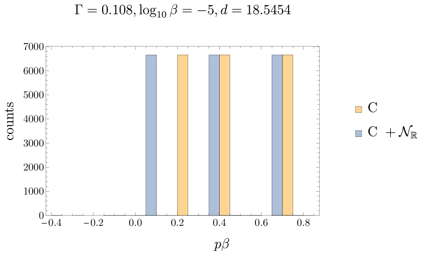
Figure 7: Although the C and $\text{C}+\mathcal{N}_{\mathbb{R}}$ models have almost identical lyapunov exponent and similar spatial behavior as apparent in this plot, the distance measure $d$ fails to capture the similarities between distributions where the peaks in the distributions are offset by small amounts.

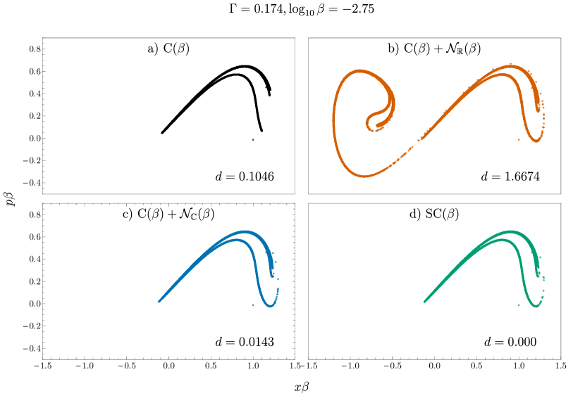
Figure 8: Different approximations are compared to the semiclassical model at the cusp of a transition from single to double well orbits at $\Gamma=0.174$, $\log_{10}\beta=-2.75$.

We note that the distance metric $d$ can yield meaningless results when comparing periodic attractors. This metric compares the distributions in $x$ and $p$, meaning that even slight displacements in sparse distributions of periodic attractors will cause the metric to diverge. An example of this is shown in Fig. 7. The models C and $\text{C}+\mathcal{N}_{\mathbb{R}}$ are quite similar and have nearly equal $\lambda$, but the distance $d=18.5454$ is really large. This pattern repeated in other examples of distances measured between periodic trajectories. For this reason, the lower bound of plots in Fig. 6 is set at $\log_{10}(\beta)=-3$, above the largest length scale at which this anomaly is present in the result.

The distance metric also fails in the vicinity of discontinuous changes of spatial behavior. The anomalous spike in $\Delta\overline{d}_{\text{SC},\text{C}+\mathcal{N}_{\mathbb{R}}}$ at $\log_{10}\beta=-2.75$ in the bottom left and right subplots of Fig. 6 is caused by a single attractor, $\Gamma=0.198$, on the cusp of a transition from a single to double well orbit. This is evident in Fig. 8, where the Poincare sections of C, $\text{C}+\mathcal{N}_{\mathbb{R}}$, and SC show trajectories constrained to the $+x$ well while the Poincare section of $\text{C}+\mathcal{N}_{\mathbb{C}}$ shows trajectory in both the $+x$ and $-x$ wells. The $\text{C}+\mathcal{N}_{\mathbb{C}}$ model jumps the gun on the discontinuous change from single to double well trajectories, resulting an anomalously high distance to SC.

Appendix C Energy Spectra Analysis

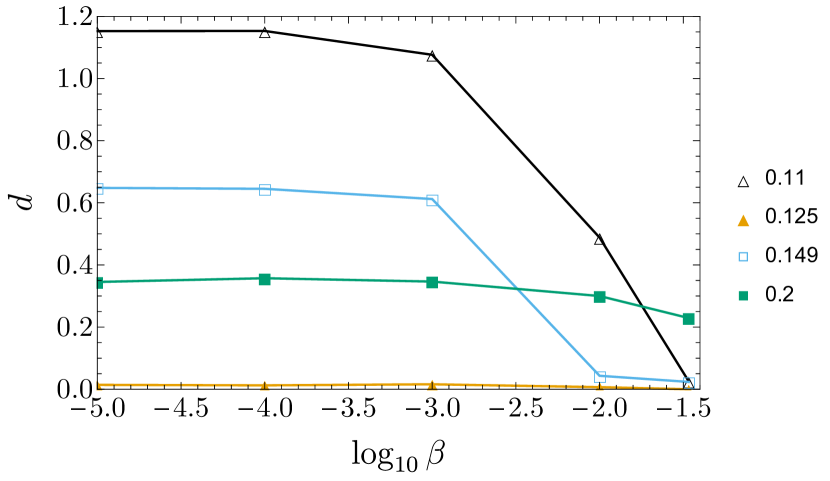
Figure 9: The distance between the energy spectra in Fig. 10 and the spectra of $\Gamma=0.125$ at $\beta_{\text{conv}}$. The distance decreases as $\beta\rightarrow\beta_{\text{conv}}$.

The convergence of attractors in the semiclassical regime is also evident in energy spectra. Fig. 10 shows energy spectra for attractors with coupling $\Gamma=0.11,0.125,0.149,0.2$ for length scales between $\beta=0.00001$ and $\beta_{\text{conv}}=0.0341$. Note that attractors ($\Gamma=0.125,0.2$) are classically chaotic and ($\Gamma=0.11,0.149$) are classically periodic. These attractors are generally representative of energy spectra in the intermediate coupling regime. The spectra are increasingly similar as $\beta\rightarrow\beta_{\text{conv}}$, although $\Gamma=0.2$ at the edge of the intermediate coupling regime is not as converged as the others. We quantify this convergence by measuring the distance $d$ between the given spectra and the spectra of $\Gamma=0.125$ at $\beta_{\text{conv}}$ (see Fig. 9). As expected, the distance decreases as $\beta$ increases, illustrating a convergence of attractors.

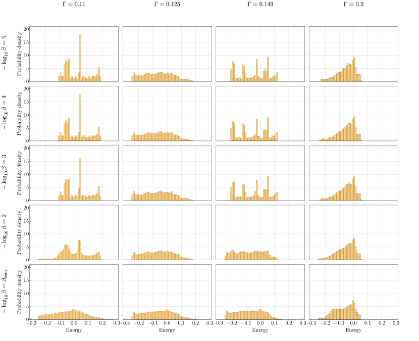
Figure 10: Energy spectra for attractors with coupling $\Gamma=0.11,0.125,0.149,0.2$ for length scales between $\beta=0.00001$ and $\beta_{\text{conv}}=0.0341$. As $\beta\rightarrow\beta_{\text{conv}}$, the spectra become more similar to one another.

Appendix D Classical noise-added models

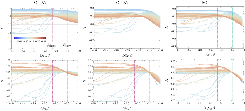
Figure 11: The $\lambda(\beta;\Gamma)$ and $K(\beta;\Gamma)$ curves for the two classical noise-added models ($\text{C}+\mathcal{N}_{\mathbb{R}}$ and $\text{C}+\mathcal{N}_{\mathbb{C}}$) and the semiclassical model (SC) over the intermediate damping regime ($0.088\leq\Gamma<0.202$). $\Gamma$ is sampled at intervals of $0.002$.

Fig. 11 shows $K(\beta;\Gamma)$ for $\text{C}+\mathcal{N}_{\mathbb{R}}$, $\text{C}+\mathcal{N}_{\mathbb{C}}$, and SC in the intermediate coupling regime. While the qualitative behavior of for the classical noise added models is similar to SC, there are noticeable differences as highlighted in the main text. The variation between the models is more pronounced as $\log_{10}\beta$ increases past $\log_{10}\beta_{\text{conv}}$. We note that the $K$ convergence is not unique to the SC model. The convergence in $K$ can be caused by simply adding classical noise to the Duffing oscillator as well; it does not require a quantum description.

Appendix E Duffing oscillator behavior in lower and higher environmental coupling regimes

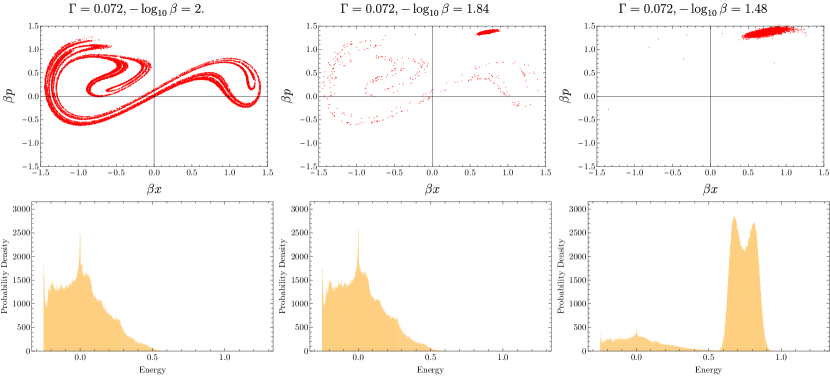
Figure 12: An example of the transition between chaotic and periodic motion for coupling levels between the low and intermediate range visualized with energy spectra and Poincare sections. Attractors in this range ($0.068\leq\Gamma<0.88$) all exhibit a similar transition.

We present our investigation of lower and higher coupling regimes here for the sake of completeness. In the low coupling regime, $\Gamma<0.068$, we observe $\lambda=-\Gamma$ in classical and most semiclassical length scales, as seen in Fig. 13. The oscillator traverses both wells in single period orbits. At high $\beta$, we observe a rise in $\lambda$ that aligns with the ‘chaotification’ of low coupling periodic orbits discovered earlier  Pokharel et al. (2018). However, these values of small $\Gamma$ and large $\beta$ are beyond the range of validity of the semiclassical formalism, and we do not attribute any physical meaning to this rapid change in $\lambda$.

Between the low and intermediate coupling regimes ($0.068\leq\Gamma<0.088$), classically chaotic orbits sharply transition to periodic behavior at some semiclassical length scale $-3<\log_{10}\beta<\log_{10}\beta_{\text{conv}}$ (see Fig. 13). During the transition from chaotic to periodic behavior, the oscillator gradually localizes to a single well and a double-peaked, high-energy cluster emerges in the energy spectra (see Fig. 12). We suspect that 1) the POs at high $\beta$ in this coupling regime are linked to the classical POs in the low coupling regime and 2) the chaotic orbits at low $\beta$ are linked to the classical chaotic orbits in the intermediate regime. Given that previous work has shown that the Lyapunov exponent is sensitive to initial conditions for some attractors in this regime Misplon and Pattanayak (2016), further exploration is warranted. The overall effect of this phenomena is that increasing $\beta$ results in a delay to the onset of chaos with respect to coupling $\Gamma$ (see Fig. 2). In the high coupling regime ($\Gamma>0.2$), $\lambda$ falls off steeply with higher $\Gamma$ (see Fig. 2). Here the oscillator is increasingly limited to a single well because of heavy dissipation through the environmental coupling. For $\Gamma\geq 0.25$, the oscillator obeys $\lambda=-\Gamma$ for much of the semiclassical regime. Similar to the low coupling regime, $\lambda$ monotonically rises at sufficiently large $\beta$.

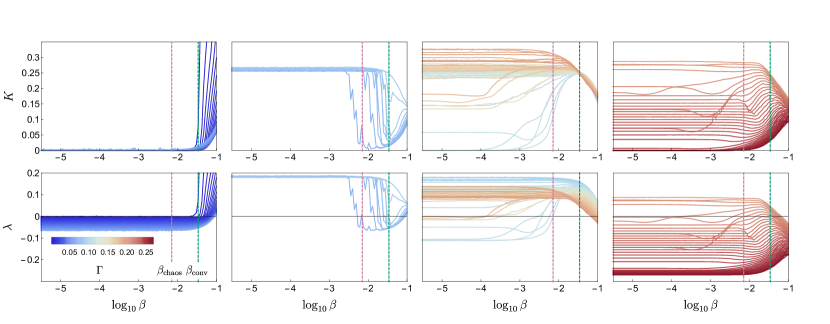
Figure 13: The top row of subplots show $\lambda$ as a function of length scale ($\log_{10}(\beta)$) for the semiclassical model over four ranges of increasing $\Gamma$ that correspond to distinct regions of behavior for $\lambda$ and $K$. The bottom row shows the same ranges of $\Gamma$ values for $K$ as a function of length scale, $\log(\beta^{-1})$.

References

- Jacobs and Landahl (2009) K. Jacobs and A. J. Landahl, Phys. Rev. Lett. 103, 067201 (2009).
- Preskill (2018) J. Preskill, Quantum 2, 79 (2018).
- Eastman et al. (2017) J. K. Eastman, J. J. Hope, and A. R. R. Carvalho, Sci. Rep. 7, 44684 (2017).
- Shi et al. (2019) Y. Shi, S. Greenfield, J. Eastman, A. Carvalho, and A. Pattanayak, in Proceedings of the 5th International Conference on Applications in Nonlinear Dynamics (Springer, 2019) pp. 72–83.
- Bakemeier et al. (2015) L. Bakemeier, A. Alvermann, and H. Fehske, Phys. Rev. Lett. 114, 013601 (2015).
- Li et al. (2012) Q. Li, A. Kapulkin, D. Anderson, S. Tan, and A. Pattanayak, Phys. Scripta T151, (2012).
- Yusipov et al. (2019) I. I. Yusipov, O. S. Vershinina, S. Denisov, S. P. Kuznetsov, and M. V. Ivanchenko, Chaos 29, 063130 (2019).
- Ghose et al. (2004) S. Ghose, P. Alsing, I. Deutsch, T. Bhattacharya, and S. Habib, Phys. Rev. A 69, 052116 (2004).
- Kumari, Meenu (2019) Kumari, Meenu, Quantum-Classical Correspondence and Entanglement in Periodically Driven Spin Systems (UWSpace, 2019).
- Pokharel et al. (2018) B. Pokharel, M. Z. R. Misplon, W. Lynn, P. Duggins, K. Hallman, D. Anderson, A. Kapulkin, and A. K. Pattanayak, Sci. Rep. 8, 1 (2018).
- Ralph et al. (2017) J. F. Ralph, S. Maskell, and K. Jacobs, Phys. Rev. A 96, 052306 (2017).
- Ott et al. (1984) E. Ott, T. M. Antonsen, and J. D. Hanson, Phys. Rev. Lett. 53, 2187 (1984).
- Dittrich and Graham (1987) T. Dittrich and R. Graham, Europhys. Lett. 4, (1987).
- Klappauf et al. (1998) B. Klappauf, W. Oskay, D. Steck, and M. Raizen, Phys. Rev. Lett. 81, (1998).
- Klappauf et al. (1999) B. Klappauf, W. Oskay, D. Steck, and M. Raizen, Phys. Rev. Lett. 82, (1999).
- Ammann et al. (1998) H. Ammann, R. Gray, I. Shvarchuck, and N. Christensen, Phys. Rev. Lett. 80, (1998).
- Pattanayak et al. (2003) A. K. Pattanayak, B. Sundaram, and B. D. Greenbaum, Phys. Rev. Lett. 90 (2003).
- Gong and Brumer (2005) J. Gong and P. Brumer, Annu. Rev. Phys. Chem. 56 (2005).
- Habib et al. (1998) S. Habib, K. Shizume, and W. H. Zurek, Phys. Rev. Lett. 80, 4361 (1998).
- Percival (1998) I. Percival, Quantum State Diffusion (Cambridge University Press, Cambridge, UK : New York, 1998).
- Brun et al. (1996) T. Brun, I. Percival, and R. Schack, J. Phys. A-Math. Gen. 29, (1996).
- Boffetta et al. (2002) G. Boffetta, M. Cencini, M. Falcioni, and A. Vulpiani, Phys. Rep. 356, (2002).
- Wolf et al. (1985) A. Wolf, J. Swift, H. Swinney, and J. Vastano, Physica D 16, (1985).
- Berman and Zaslavsky (1978) G. P. Berman and G. M. Zaslavsky, Physica A 91, 450 (1978).
- Prezhdo (2002) O. V. Prezhdo, J. Chem. Phys. 117, 2995 (2002).
- Tomsovic and Heller (1991) S. Tomsovic and E. J. Heller, Phys. Rev. Lett. 67, 664 (1991).
- Banerjee et al. (2004) D. Banerjee, B. C. Bag, S. K. Banik, and D. S. Ray, The Journal of Chemical Physics 120, 8960 (2004).
- Pattanayak and Schieve (1994) A. Pattanayak and W. Schieve, Phys. Rev. E 50, (1994).
- Misplon and Pattanayak (2016) M. Z. R. Misplon and A. K. Pattanayak, “Investigation of co-existing attractors in the duffing oscillator,” (2016), unpublished.