Which model features matter? An experimental approach to evaluate power market modeling choices

Abstract

A novel experimental approach of inter- and intramodel comparisons is conducted with five power market models to give recommendations for modelers working on decarbonization pathways of Europe until 2050. The experiments investigate the impact of model type (optimization vs. simulation), planning horizon (intertemporal vs. myopic), temporal resolution (8760 vs. 384 hours), and spatial resolution (28 countries vs. 12 mega-regions). The model type fundamentally determines the evolution of capacity expansion. Planning horizon (assumed foresight of firms) plays a minor role for scenarios with high carbon prices. For low carbon prices in turn, results from myopic models deviate considerably from those of intertemporal models. Lower temporal and spatial resolutions foster wind power via storage and via neglected transmission boundaries, respectively. Using simulation instead of optimization frameworks, a shorter planning horizon of firms, or lower temporal and spatial resolutions might be necessary to reduce the computational complexity. This paper delivers recommendations on how to limit the discrepancies in such cases.

1 Introduction

The European energy system has grown in complexity over the past decades: Liberalization broke up integrated energy suppliers and led to a variety of energy market participants. Decarbonization efforts continue to transform the electricity supply [1], particularly towards a more spatially distributed system through the rise of renewable energy sources. Furthermore, electricity demand is set to increase since electrification is a major means of decarbonizing the transport and heat sectors [2]. Within this increasingly complex system, numerical power market models gain importance in assessing future developments and the impact of different policies. In order to provide robust, evidence-based policy recommendations, a fundamental understanding of the numerical models is crucial.

Power market models are increasingly sophisticated and include a variety of features with superposed, often contradictory effects [3]. Additionally, there are multiple model formulations, different data sources, and various scenarios that can be used to answer the same policy question. To gain more clarity on the behavior of models and avoid contradictory recommendations, it is necessary to conduct model comparisons, preferably with harmonized features, same input data, and consistent scenarios. The harmonization of features, data, and scenarios reduces the differences between the models to the core features and renders the causal inference possible, which ultimately increases the confidence in the modeling methods.

Five power market model frameworks are compared using harmonized input data and features. All models are dispatch and investment models that expand generation capacity in the European power market (EU27 plus Norway, Switzerland, and United Kingdom, without Cyprus and Malta) from 2015 (base year) to 2050 (model horizon) in 5-year steps. The harmonization process starts with the handling of a joint database to ensure valid results. Several optional features are then deactivated to create frameworks with similar capabilities. The data and feature harmonization is crucial because it allows the attribution of remaining deviations in results to four key features of power markets models: model type, planning horizon, temporal resolution, and spatial resolution. Finally, differences between the models are assessed in several experiments, each focusing on one of those features.

The four above mentioned features are critical for power market models. Model type determines whether firm behavior is reflected by profit maximization or cost minimization (i.e., optimization), or by decision heuristics (i.e., simulation). Planning horizon covers the assumed foresight of firms, and is either myopic (i.e. short-sighted, dealing with each time period separately) or intertemporal (taking into account all time periods simultaneously). Whereas model type and planning horizon reflect general stakeholder behavior, temporal and spatial resolutions have an impact on the level of detail and the computational complexity. Supply from intermittent renewable energy sources and electricity demand fluctuate over space and time. Storage and transmission, which can balance these fluctuations, are limited. As a consequence, power market models need to reflect these constraints by striking a balance between the model resolution and its solving time.

The main results are threefold. First, the used simulation model with its current formulation is both slow in exiting conventional technologies (e.g. nuclear and coal) and fast in adopting new technologies, even when their usage is not economically profitable yet. Second, myopic models perform well in comparison to intertemporal models. Although intertemporal models tend to wait longer to exploit sites with high variable renewable energy (VRE) potentials using efficient technologies, overall VRE expansion is similar by 2050. Third, wind output is higher for lower temporal and spatial resolutions due to overestimated storage capabilities when using typical time steps (in contrast to 8760 hours of a year) and missing transmission line contingencies within grouped countries. For the sake of transparency, the harmonized input data as well as the derived results are provided. Hence, other modelers are able to benchmark their models against the used ones.

The next section explores related literature and compares the adopted approach to other model comparisons. Section 3 describes the model frameworks, model features, and the data harmonization process. Section 4 describes the experiments with their settings and results. Section 5 concludes.

2 Literature

At the core of this paper is a novel experimental approach to compare numerical power market models, which has not been done before to that extent with regard to feature and data harmonization. The five models involved were part of the 4NEMO project, which provided the necessary resources to conduct the analysis. Table 1 gives an overview of reviews, as well as intramodel and intermodel comparisons in the field of energy system modeling. To distinguish between intramodel and intermodel comparisons, the difference between frameworks and models is first clarified: whereas a framework is an abstract set of code, a model is an instance of that code combined with actual data for a specific problem. Hence, intramodel comparisons rely on a single framework with multiple model instances, whereas intermodel comparisons involve different frameworks.

The table also assesses the level of data harmonization, the number of considered model frameworks, and whether or not the papers analyze the impact of model type, planning horizon, temporal resolution, and spatial resolution, as is done in this paper.

Reviews discuss qualitative properties and usually cover a wide spectrum of model frameworks with multiple variations. They support decision-makers in selecting suitable model frameworks for answering specific policy and research questions [4]. In general, they classify models [5] or identify current challenges and trends in the literature [6]. A better overview of the model landscape further aids researchers in identifying research gaps [7]. However, reviews cannot quantify the impact of different model, feature, or data choices on the outcomes. To this end, model comparisons are carried out.

Table 1: Literature review. Dashes (–) mean that the attributes are not applicable.

Ref.	Comparison type	Harmo-nization	Nr.	Model types	Planning horizon	Temporal resolution	Spatial resolution
[4]	Review	–	21	O	I, M	–	–
[5]	Review	–	22	O, S	I, M	X	X
[6]	Review	–	37	O, S	I, M	X	X
[7]	Review	–	40	O, S	I, M	–	–
[8]	Intramodel	–	1	O	–	–	–
[9]	Intramodel	–	1	O	M	X	–
[10]	Intramodel	–	1	O	I	X	–
[11]	Intramodel	–	1	O	M	X	X
[12]	Intramodel	–	1	O	M	X	X
[13]	Intramodel	–	1	O	M	X	–
[14]	Intermodel	Low	6	E, O, S	–	–	–
[15]	Intermodel	Low	7	E, O, S	I, M	–	–
[16]	Intermodel	Low	10	O, S	I	–	–
[17]	Intermodel	Low	10	O, S	I	X	X
[18]	Intermodel	High	2	O	I	X	–
[19]	Intermodel	High	2	O	I	X	–
[20]	Intermodel	High	2	O	M	X	–
[21]	Intermodel	High	4	O	M	X	X

Intramodel comparisons apply several model configurations to a single model framework and evaluate their effects on the model outputs. Ommen et al. [8] compare different complexity levels of modeling formulation, i.e., linear, mixed integer, and non-linear, within a generic dispatch model framework. Pfenninger [9] and Nahmacher et al. [10] evaluate the impact of the selection of representative time slices, while Frew and Jacobson [11] and Priesmann et al. [12] assess the trade-off between spatial and temporal resolution systematically. Diaz et al. [13] analyze the importance of modeling complexity in long-term energy planning models in terms of time resolution, operational inflexibility and uncertainty regarding fossil fuel prices. A clear advantage of intramodel comparisons is that there is no need for data harmonization. However, considering only one framework neglects the effects of its inherent characteristics.

Intermodel comparisons are carried out on model frameworks and help to evaluate the robustness of findings. Some intermodel comparisons derive robust climate change mitigation trends and strategies that remain valid regardless of the applied model framework, such as Van Vuuren et al. [14] comparing bottom-up and top-down mitigation potentials estimates, Capros et al. [15] applying different technological and policy choices, Förster et al. [16] looking into European energy efficiency, and Knopf et al. [17] looking into decarbonization strategies beyond 2020. Those papers involve a high number of models, but the level of input data harmonization is lower in contrast to the experimental approach presented here. Other intermodel comparisons analyze modeling details by comparing only two (examples: Deane et al. [18] about soft-linking, Kiviluoma et al. [19] on the value of renewable generation, and Poncelet et al. [20] on the impact of modeling detail) or four models [21] with highly harmonized data. The latter is the most similar approach from literature to this paper. It presents a systematic model comparison between energy system models based on linear optimization with focus on temporal and spatial resolution as well as sector coupling. The analysis includes three scenarios for the German power supply system in 2050. Unlike this approach, the comparison presented here includes a simulation model with heuristic-based investment decisions alongside optimization models with cost-minimizing objective functions. By extending the planning horizon to more than one year, this paper also investigates the impact of the choice between a myopic and an intertemporal approach.

Based on the evidence from the literature, the following conclusions can be drawn. First, most model comparisons are either purely intramodel or intermodel, but not both. Second, while the impact of the temporal resolution is prominent in most papers, the other categories are not well researched. Investigating the spatial resolution features only in a few, and only Capros et al. [15] evaluate the impact of the planning horizon. Different model types are only compared in intermodel comparisons with low harmonization levels. Third, the level of harmonization for intermodel comparisons of more than two models is typically low, with Gils et al. [21] being the only exception. This paper contributes to the prevalent literature by quantifying the impacts of model type, planning horizon, and temporal and spatial resolutions in a highly harmonized intermodel comparison. Thereby, it fills the described gaps in the existing literature.

3 Frameworks, data, and model features

This section first introduces the models involved in the model comparisons. This is followed by a description of the data. Finally, the model features are classified into major features, deactivated features, and remaining differences.

3.1 Model frameworks

All considered frameworks (see Table LABEL:tab:frameworks) are partial equilibrium models that cover (most of) the interconnected European power markets (28 countries: EU27 excluding Cyprus and Malta, including Norway, Switzerland, and the United Kingdom). Trade between markets is possible via transmission lines. The frameworks include a detailed depiction of different thermal power plants (e.g., efficiency, emission factor, year of installation, lifetime and planned decommissioning), intermittent and other renewable energy technologies, and storage. The model frameworks decide on dispatch and investments by using exogenous assumptions on the development of electricity demand, fuel prices, and techno-economical characteristics of the considered technologies. Within those characteristics, technological progress is depicted via vintage classes based on the commissioning year of the technologies.

Table 2: Considered model frameworks.

Name	Institution	Type	Software	References
DIMENSION	Institute of Energy Economics at the University of Cologne	Optimization	GAMS, CPLEX	[22]
EUREGEN	ifo Institute for Economic Research	Optimization	GAMS, CPLEX	[23]
E2M2	Institute of Energy Economics and Rational Energy Use	Optimization	GAMS, CPLEX	[24]
urbs	Chair of Renewable and Sustainable Energy Systems	Optimization	Pyomo, Gurobi	[25]
HECTOR	Institute for Future Energy Consumer Needs and Behavior	Simulation	Vensim	[26]

3.2 Data harmonization

A database developed within the 4NEMO project, which contains all essential data for modeling different futures of an interconnected Europe, i.e., scenario assumptions and technology data, is used (see A for an overview of the most relevant numerical assumptions).

Scenario assumptions

The assumptions cover fuel and carbon prices, electricity demand, and net-transfer capacity (NTC) expansion. One out of the four scenarios developed within the 4NEMO project is used in this paper [27]. The chosen scenario, Stagnation of the EU, describes a collaborative future to reach ambitious climate targets. The development of emissions stringency and grid interconnections is retrieved from expert interviews using the cross-impact balance method [28]. Fuel prices and electricity demand were quantified by using the computational general equilibrium (CGE) model PACE [29]. Despite improvements in energy efficiency, the electricity demand roughly doubles (+105%) until 2050 due to direct and indirect electrification of transport, services, manufacturing, and energy intensive industries (see Table 6). This increase is in the higher end of the range spanned by similar studies (+66% in [30], +80%–150% in the ambitious scenarios of [31]). Nevertheless, this scenario is used because the demand increase pushes the models to exploit more renewable resources and thus triggers differences in results which are interesting for the model comparison.

This scenario assumes that carbon prices (within the EU ETS) rise to 132 EUR/t_CO2 in 2050 (see Table 3) and that interconnectivity remains at the 2030 level in accordance to the 10-year development plan. This paper further considers the following variations:

• lower CO₂ price: Carbon price of 44 EUR/t_CO2 in 2050

• higher CO₂ price: Carbon price of 176 EUR/t_CO2 in 2050

• increased NTC: Interconnectivity targets beyond 2030 increase to 25%

Technology data

This data covers information about existing infrastructure (generation, storage, and transmission capacities) as well as their projected expansion.

The database provides assumptions about past (1960 to 2010), current (2015), and future (2020 to 2050) techno-economic parameters. It includes ten different thermal plants (lignite, coal, coal with CCS, nuclear, solid bioenergy, solid bioenergy with CCS, open-cycle gas turbines, combined-cycle gas turbines, steam turbines with natural gas, geothermal). The technologies differ with regards to their key technology-specific characteristics (efficiency, reliability, capacity credit, CO₂ emission factor, CO₂ capturing factor for CCS technologies, commissioning year, lifetime, depreciation period, variable and fixed operations and maintenance cost, investment cost). Bioenergy and CCS technologies are restricted by country-specific bioenergy or carbon-storage potentials, respectively. In line with current political announcements, investments into nuclear power are restricted to Eastern Europe, France, Scandinavian countries, and the United Kingdom.

The database further contains eight different intermittent renewable technologies (hydro power plants, three different onshore wind and three different offshore technologies, solar PV) with potentials and hourly availabilities (i.e. capacity factors) based on Siala and Houmy [32]. The hourly capacity factors are deterministic. Wind and solar technologies are differentiated into three resource quality classes – high, medium, and low – which reflect the geographic diversity of each region. The time series of each region were generated for multiple representative sites with predefined quality levels, then weighted so that the wind and solar generation are calibrated to historical data. Curtailment is endogenously determined and eventually reduces the yearly capacity factors of intermittent renewable technologies, which are limited by the harmonized availability factors for each technology, site, and resource quality class. This means that the models may not use all the renewable energy that is available in every time step, if its integration leads to higher costs, for example through the construction of transmission lines and storage. Finally, transmission capacity is approximated by using net-trade capacities.

3.3 Major differences

The model frameworks are compared with regard to four major differences of power market models: (1) model type, (2) planning horizon, (3) temporal resolution, and (4) spatial resolution.

Model type

There is a differentiation between optimization and simulation frameworks. Optimization frameworks decide on dispatch and investment by minimizing overall system costs (variable, fixed operation and maintenance, as well as investment cost). The considered simulation framework (HECTOR) determines dispatch based on variable costs, but uses a heuristic for investment decisions.

The considered optimization model frameworks (DIMENSION, EUREGEN, E2M2 and urbs) rely on the fundamental assumptions of perfectly competitive markets, symmetric firms with homogeneous information and cost structures, and no transaction cost. Representative firms seek to maximize their profits, which, under the above mentioned fundamental assumptions, is equivalent to a minimization of total system cost. Consequently, optimization models represent idealized depictions of real power markets.

Simulation models allow to break the fundamental assumptions described above. For example, HECTOR abstracts from perfect competition, assuming that firms might skim off scarcity rents in hours where available capacity is scarce. In doing so, HECTOR tries to depict peak pricing in peak-load hours more realistically. Deviating from idealized markets, however, requires HECTOR to solve the underlying problem iteratively.

Planning horizon

The planning horizon reflects the foresight in investment behavior. Intertemporal models assume perfect foresight and thus can avoid path dependencies and lock-in effects by calculating dispatch and investment decisions considering the entire time horizon. Myopic models in turn do not avoid eventual path dependencies and lock-in effects. Such models divide the optimization problem into sub-problems, which are solved consecutively. Under myopia, dispatch and investment decisions in a certain period are made without the knowledge of future investment periods. The results obtained from the optimization of the respectively prior periods are taken as input to optimize the current period.

Temporal resolution

This feature defines how many time steps are used to reflect the fluctuations within a year. In general, two approaches can be differentiated: Fully depicting a year using 8760 hourly time steps, or using representative hours which are chosen heuristically or through clustering. A full depiction preserves all the information about the fluctuations of the load and renewable generation profiles. Representative time steps reflect the most significant patterns and reduce model complexity significantly. However, representative hours may struggle in accurately modeling storage behavior (Nahmacher et al. [10]).

In this paper, a full year depiction (8760 hours) is compared to the use of 16 representative days (384 hours). Due to the computational complexity, intertemporal models were only able to perform the runs with 384 time steps. Simplified time series are scaled so that the annual demand and full-load hours of intermittent technologies match those of full temporal resolution.

Spatial resolution

This feature describes the number and shape of the model regions. It is normally a flexible parameter that varies according to the research question. The most intuitive spatial resolution for power market models equals the spatial configuration of the depicted wholesale power markets. For most European countries, market configuration is congruent with national borders, while a few countries are split into several markets (e.g. Norway, Sweden).

A country-wise depiction (28 regions) is compared to a setting where the countries are aggregated into 12 mega-regions. Using the ISO 3166-1 alpha-2 codes: DE, FR, and IT are modeled as single countries. DK, FI, NO and SE are grouped into one region. Other regions are AT-CH, BE-LU-NL, BG-EL-RO, CZ-PO-SK, EE-LT-LV, ES-PT, HR-HU-SI, and IE-UK.

3.4 Deactivated and non-modeled features

First, several framework-specific features are deactivated for the sake of data harmonization. The focus is on wholesale power markets, and thus there is no depiction of other energy-related markets (e.g., balancing power or CO₂ markets) or other sectors (e.g., heat or transport). Framework-specific selection and weighting algorithms are deactivated since harmonized time series for electricity demand and intermittent renewable generation) with either 384 or 8760 time steps are used.

Next, there is no depiction of direct subsidies (feed-in tariffs, market premiums, capacity payments) and indirect subsidies (renewable energy share targets, priority dispatch). In principle, all considered models are able to model different forms of subsidies although those features are rarely activated.This assumption is particular valid for the European power market because the major climate policy that drives system transformation is the CO₂ price from the EU Emissions Trading System (EU ETS). The considered CO₂ price stems from a CGE calibration that seeks to model all policies projected by the European Joint Research Centre, that is, the price covers more than just the quantity target from the EU ETS but rather accounts for different implemented policies such as direct and indirect subsidies and taxes as well. Thus, the focus is on testing sensitivity of experiment outcomes for diverging CO₂ price paths without adding any overlapping, substituting, or even contrary policies such as direct and indirect subsidies, which often differ by country and might hamper the comparability of models.

Finally, technological constraints such as minimum dispatch, ramp-up restrictions, and unit commitment are not used. All considered models are principally able to depict minimum dispatch, but refrain from doing so because technology capacities are actually aggregated by vintages in each model (by the period of installation in five year steps). A minimum dispatch constraint is therefore often more restrictive for vintages that have sizes above the regular power plant size. Gils et al. [33] show that such constraints have a minor impact and Ramachandran et al. [34] find that ramping restrictions do not matter for long-run capacity expansion. Regarding unit commitment, it cannot be depicted by any of the used models, at least not in their present specifications.For such purpose, mixed-integer program unit commitment models are used [e.g., 35].

3.5 Remaining differences

Some features are fundamental for the working of the respective model framework. Those features are kept active, although not all model frameworks were able to account for them.

Endogenous decommissioning

Only the two model frameworks with intertemporal versions (DIMENSION and EUREGEN) allow to retire power plant, transmission, and storage capacities before the end of their technical lifetime.

Technology aggregation

To ensure numerical feasibility, DIMENSION additionally reduces the number of vintages (for existing and newly built capacity) by merging every three vintages into one mega-vintage, for example the mega-vintage class 1960–1974 replaces 1960–1964, 1965–1969 and 1970–1974.

Storage

Storage is deactivated in HECTOR. The framework is generally able to model it, but the way of doing so is incomparable with the way the other models do.

Negative emissions

E2M2 is not capable of handling revenues from negative emission technologies. As a result, there is no benefit from investing in bioenergy with CCS, even though it is technically allowed.

Limits for renewable potentials

The capacity expansion of solar and wind is limited by the total potential minus the existing capacities over all vintages. Since E2M2 cannot determine this variable endogenously, it sets exogenous upper bounds for each year that are constant over time.

4 Model experiments

This section encompasses all the experiments used for the model comparison, starting by a benchmarking experiment followed by one experiment for each major model feature.

4.1 Benchmarking experiment

Experiment setup

Each model involved in this experiment uses a particular configuration of major features, which the modeler considers as basic setup. The models use the same harmonized input data for the scenario base, modeling the European power market in 5-year steps between 2015 and 2050. Capacity expansion is only allowed after 2015.

Table 3: Models used in the benchmarking experiment.

Model variation	Optimization	Simulation	Intertemporal	Myopic	Full year	Typical steps	28 countries	12 mega-regions	Model framework
OIT28-D	X		X			X	X		DIMENSION
OIT12-R	X		X			X		X	EUREGEN
OMY12-E	X			X	X			X	E2M2
OMY28-U	X			X	X		X		urbs
SMT12-H		X		X		(X)		X	HECTOR

Results

The comparison of the evolution of the electricity mix in Figure 1 shows that the results are not similar. Large differences start to appear in 2020, when endogenous expansion is allowed. The models disagree on when to phase out coal (OIT28-D: 2040, SMT12-H: beyond 2050), when to build gas CCS power plants (SMT12-H: 2025, OMY28-U: 2045), and on the share of onshore wind in 2050 (OMY12-E: 30.6%, OIT28-D: 57.0%), to name a few examples. The differences are also reflected in the total system costs and on the CO₂ emissions (see Supplementary materials [36]).

Key message

Since all models use the same harmonized input data, the differences must be due to the configuration settings of the model frameworks (major features) and/or due to the mathematical formulations of the specific model features. Therefore, the next experiments are designed to estimate the impact of the model features on the results.

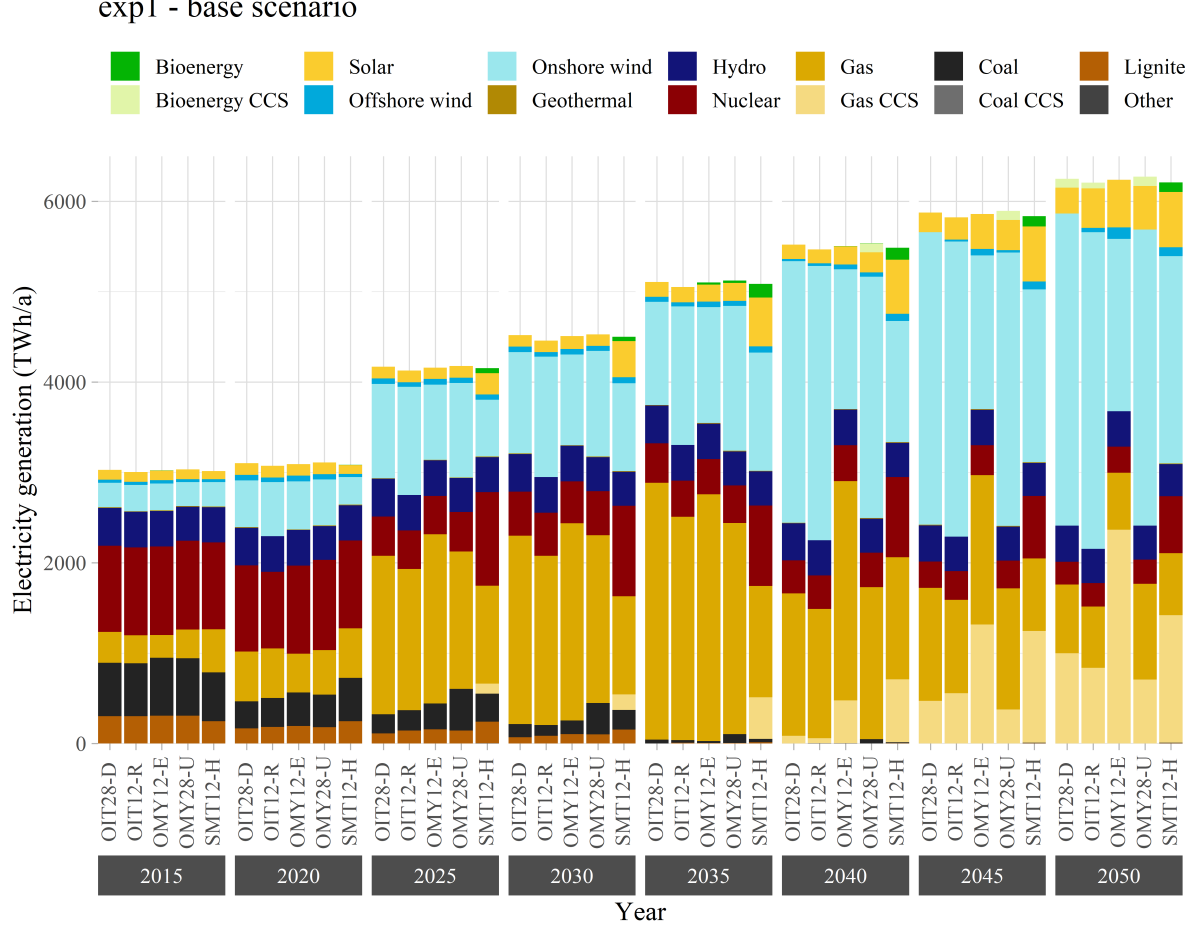
Figure 1: Electricity generation over the period 2015-2050 for all models involved in the benchmarking experiment.

4.2 Impact of model type

Experiment setup

Apart from the feature “model type”, all the other major features are harmonized. The compared models are myopic, they use 384 typical time steps, and they consist of 12 mega-regions. Table 4 provides an overview of the used models.

Table 4: Models used in the model type experiment.

Model variation	Optimization	Simulation	Intertemporal	Myopic	Full year	Typical steps	28 countries	12 mega-regions	Model framework
OMT12-D	X			X		X		X	DIMENSION
OMT12-R	X			X		X		X	EUREGEN
OMT12-E	X			X		X		X	E2M2
OMT12-U	X			X		X		X	urbs
SMT12-H		X		X		(X)		X	HECTOR

Results

The difference between the optimization models and the simulation model is most striking in the evolution of the installed capacities, which is displayed in Figure 2. Whereas myopic optimization models make investment decisions endogenously based on annualized total costs, the simulation model HECTOR uses a heuristic investment decision module for new capacities. This module expands all technologies with a positive net present value (NPV) and assigns investment shares to them based on (i) the total capacity of each region, (ii) the ratio of expected NPV to total investment costs, and (iii) on user-defined parameters. The calculation of the NPV requires additional assumptions on the expected full-load hours of each power plant type. This explains why the simulation model starts investing in gas power plants with CCS from 2025, or why it keeps investing in new nuclear capacities until 2050, even though these power plants will probably operate less often than expected due to the high share of renewable generation. The non-optimal allocation of new capacities leads to higher total system costs, which exceed the average costs of optimization models by 50% in 2050.

The results of the optimization models are similar, yet not identical. In particular, the non-modeling of negative CO₂ emissions in E2M2 justifies the absence of bioenergy CCS in 2050. Also, the exogenous constraint on the yearly increase of renewable capacities in the same model might explain why its results show a lower capacity of onshore wind by 2050.

Sensitivity to other scenarios

If the CO₂ price increases faster, the optimization models build negative emissions technologies (bioenergy and gas CCS) as soon as 2035, and install more onshore wind instead of conventional gas power plants. If the price increase is moderate, no negative emissions technologies are built, coal is used until 2050, and less solar and onshore wind power plants are built. The simulation model is barely sensitive to the increase of CO₂ price, since its energy mix and the shares of new installed technologies remain unchanged. However, the absolute values of the installed capacities in the scenario with lower CO₂ price increase because of two mutually reinforcing effects. On the one hand, the installed capacities of conventional power plants (e.g., gas) increase because they are cheaper. On the other hand, a system with higher dispatchable generators allows to integrate more renewable energy capacities. This is due to the way market frictions and investment dynamics are depicted in HECTOR.

Key messages

The type of the model is a core difference that has a large impact on the results. Whereas the simulation model in this experiment can replicate the operation of a diverse portfolio of technologies, its investment decisions are very different from optimization models. The system suggested by the simulation model includes innovative technologies (e.g., gas CCS) earlier, and relies on conventional technologies (e.g., coal) for a longer period. It is also less sensitive to CO₂ price variations. The differences are down to the fact that the simulation model relies on a large number of user-defined parameters for its investment module, rather than a difference in paradigms between optimization and simulation. Capros et al. [15] observe a similar behavior regarding the integration of CCS and the deployment of nuclear and coal, and recommend performing sensitivity analyses to validate the assumptions of simulation models.

The diversity in modeling approaches reveals the synergy between them: simulation models could use optimization results to calibrate their parameters and reduce the number of runs, then deliver electricity prices and other outcomes that better reflect existing imperfections in power markets.

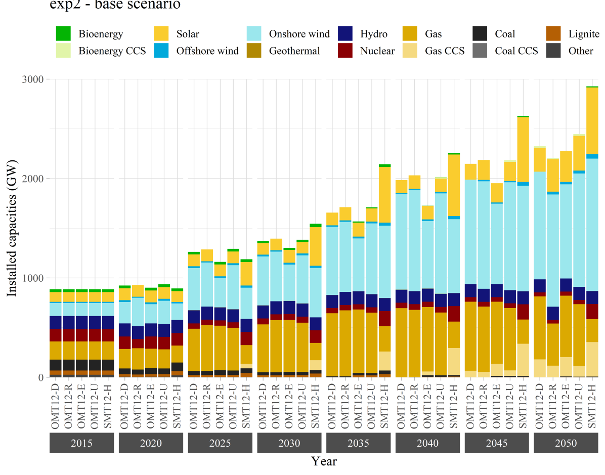
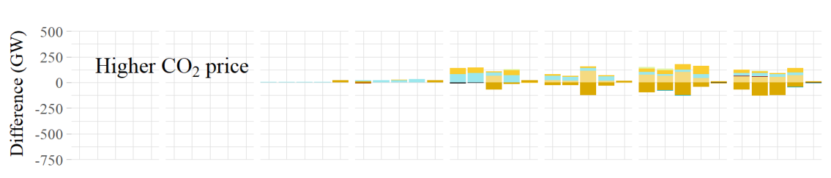
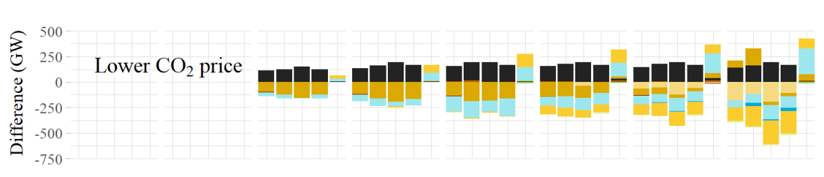
Figure 2: Total installed capacity in the period 2015-2050 for all models involved in the model type experiment (top) and differences due to higher and lower CO₂ prices (bottom).

4.3 Impact of planning horizon

Experiment setup

Apart from the feature “planning horizon”, all the other major features are similar. Only models based on the frameworks DIMENSION and EUREGEN are compared, as only they provide the option to vary the planning horizon. The compared optimization models use 384 typical time steps and consist of 12 mega-regions. Table 5 provides an overview of the used models.

Table 5: Models used in the planning horizon experiment.

Model variation	Optimization	Simulation	Intertemporal	Myopic	Full year	Typical steps	28 countries	12 mega-regions	Model framework
OIT12-D	X		X			X		X	DIMENSION
OMT12-D	X			X		X		X	DIMENSION
OIT12-R	X		X			X		X	EUREGEN
OMT12-R	X			X		X		X	EUREGEN

Results

Figure 3 compares the evolution of the electricity generation mixes of the four models. Intramodel differences are first analyzed by observing the results of each pair of models from the same framework.

Both in 2015 and 2050, the differences between the models of the same framework are minor (the largest differences in onshore wind generation in 2050 are of 120 TWh/a for DIMENSION and 170 TWh/a for EUREGEN in 2050, so less than 2% and 2.7% of the generation, respectively). However, there are discrepancies for the years in between. For both frameworks, the myopic versions have a higher share of onshore wind between 2025 and 2035, which the intertemporal models replace with gas. From 2040 onward, the model OIT12-D builds gas CCS plants and uses more onshore wind and less conventional gas power plants than its myopic counterpart. OIT12-R also builds onshore wind at a large scale after 2040. This could be explained by the limits on the potential of onshore wind expansion. Since the intertemporal models have perfect foresight, they do not exhaust the wind potential until a new generation of more efficient wind turbines becomes available in 2040. This is at odds with other papers that show intertemporal models investing earlier in low-carbon technologies [37], but the outcomes can plausibly be justified by the exogenous technological progress (which is actually only possible if there is high adoption of the technology in previous years) and the potential constraints for onshore wind.

The intertemporal models minimize the costs over the whole time horizon, whereas the myopic ones optimize the system design and operation for each period separately. Consequently, the system costs over the period 2015–2050 must be higher in the myopic models than in the intertemporal models (or at least equal). This is confirmed in this experiment, albeit the difference is marginal (DIMENSION: +1.0%, EUREGEN: +1.6%).

The reasons for the different behaviors in DIMENSION and EUREGEN could be traced back to aspects that have not been harmonized, such as technology vintage aggregation in DIMENSION or the exact implementation of endogenous decommissioning.

Sensitivity to other scenarios

If the CO₂ price increases faster, the myopic models deliver solutions that are +1.5% (OMT12-D) and +2.1% (OMT12-R) more expensive than their intertemporal counterparts, while the energy mix does not vary considerably. While myopic and intertemporal models show similar behavior in the base as well as in the +CO₂ scenario, the investment horizon becomes crucial under lower carbon prices. If the CO₂ price increases slowly, the model OMT12-D uses coal power plants to cover 10–20% of the energy demand from 2035 onward. In that scenario, the difference in system costs between OMT12-D and OIT12-D reaches +2.3%, and +2.5% for OMT12-R and OIT12-R. Under myopia, low carbon prices in the short-run lead to investments in new coal power plants. Models with perfect foresight anticipate that these investments will not pay off over the lifetime of the power plants since carbon prices will increase. Thus, intertemporal models rely on gas power plants instead.

Key messages

Intertemporal and myopic models might agree on the optimal energy mix in the long term, but they disagree on the way to get there. Due to their perfect foresight, intertemporal models can take into consideration constraints that span over time (e.g., renewable potential constraints), or that change over time (e.g., CO₂ price), and make investment decisions accordingly. The lack of this capability in myopic models leads to slightly higher overall costs, but the gap widens for scenarios with lower CO₂ constraints. Assuming that policy makers consider similar long-term scenarios, they could compare the costs in both models and decide whether the difference justifies a regulatory intervention to control the wind expansion, for example.

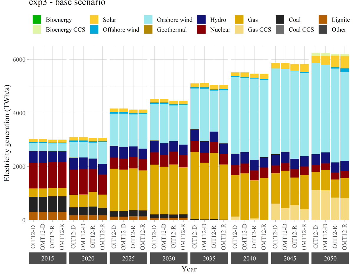
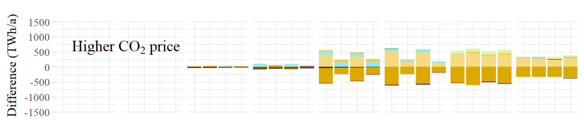
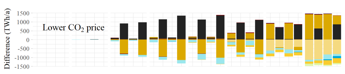
Figure 3: Electricity generation over 2015-2050 for the models involved in the planning horizon experiment (top) and differences due to higher and lower CO₂ prices (bottom).

4.4 Impact of temporal resolution

Experiment setup

Apart from the feature “temporal resolution”, all the other major features are similar. The compared optimization models are myopic and consist of 12 mega-regions. They either use 8760 time steps (full year) or 384 (typical steps). For the latter case, four consecutive days from different seasons were chosen. The models use the same time steps. Only the frameworks E2M2 and urbs are involved in this experiment because they have the computational infrastructure to run optimizations with 8760 time steps. Table 6 provides an overview of the used models.

Table 6: Models used in the temporal resolution experiment.

Model variation	Optimization	Simulation	Intertemporal	Myopic	Full year	Typical steps	28 countries	12 mega-regions	Model framework
OMT12-E	X			X		X		X	E2M2
OMY12-E	X			X	X			X	E2M2
OMT12-U	X			X		X		X	urbs
OMY12-U	X			X	X			X	urbs

Results

Analogously to the previous experiment, the intramodel differences are first analyzed by observing the results of each pair of models from the same framework. Figure 4 compares the evolution of the electricity generation mixes of the four models, and their usage of storage devices.

In both frameworks, it is observed that the models with fewer time steps rely more on onshore wind generation, which the 8760-time-step models replace in part with gas, gas CCS and solar generation. For instance, the share of onshore wind in electricity generation in 2050 is 47% in OMT12-E and 30.6& in OMY12-E, whereas the combined share of gas, gas CCS and solar shifts from 40,2% to 56.6%, respectively. The higher reliance on onshore wind occurs in conjunction with a higher usage of storage, in particular long-term storage. In fact, the share of long-term storage in OMT12-E and OMT12-U (27.8% and 8.5%, respectively) is greater than its share in OMY12-E and OMY12-U (25% and 4.1%, respectively). In absolute terms, most of the storage occurs in pumped hydroelectric storage up until 2040 (63.5% and 69.5% in 2040 in OMT12-U and OMY12-U, respectively), then in short-term storage devices (61.7% and 61.6% in 2050 in OMT12-U and OMY12-U, respectively).

The discrepancy between the models has two explanations. First and foremost, the reduction of the number of time steps necessarily impacts the shape of the time series, i.e., their hourly fluctuations. In this experiment, the time steps were selected heuristically, not through clustering and weighting of the clustered patterns. The time series were scaled and stretched to ensure that the total electricity demand and the full load hours of wind and solar generation are preserved. This process alters the shape of the time series, and affects each one independently of the others, so that the temporal correlation between weather and load events is not preserved. Clearly, this effect has favored onshore wind generation in this experiment.

Second, the way storage is modeled has an impact on the results. In all four models, the equations describing the storage state depend on its state in the previously modeled time step. In the absence of a mechanism to account for gaps between physically distant time steps in the models with 384 time steps, transitions between seasons are neglected. Consequently, the models inevitably overestimate the need for long-term, seasonal storage, which also favors the use of onshore wind.

One major difference between E2M2 and urbs models consists in the modeling of wind expansion. E2M2 splits the wind expansion potential into evenly distributed yearly portions, which remain unused in the first years and are not transferred to future years. It compensates for the lack of wind generation from 2040 onwards by using gas CCS with long-term storage more often than urbs. The fact that the model uses long-term storage to boost the full load hours of gas CCS seems counter-intuitive, since short-term storage is much cheaper per MW and is more efficient. However, the high energy-to-power ratio of long-term storage (720 MWh/MW to 4 MWh/MW) allows a much more cost-effective shifting of energy despite higher storage losses. The reliance on long-term storage makes E2M2 models more sensitive to the change of the temporal resolution.

Key messages

The impact of the temporal resolution is correlated with the quality of the complexity reduction technique. If the reduction of the time steps does not preserve the temporal correlation of the demand and renewable supply time series, variations in the share of renewable technologies might occur. The experiment echoes the recommendations of Nahmacher et al. [10] regarding the impact of the choice of time steps. In case irregular time gaps are not accounted for in storage modeling, the variations might be amplified.

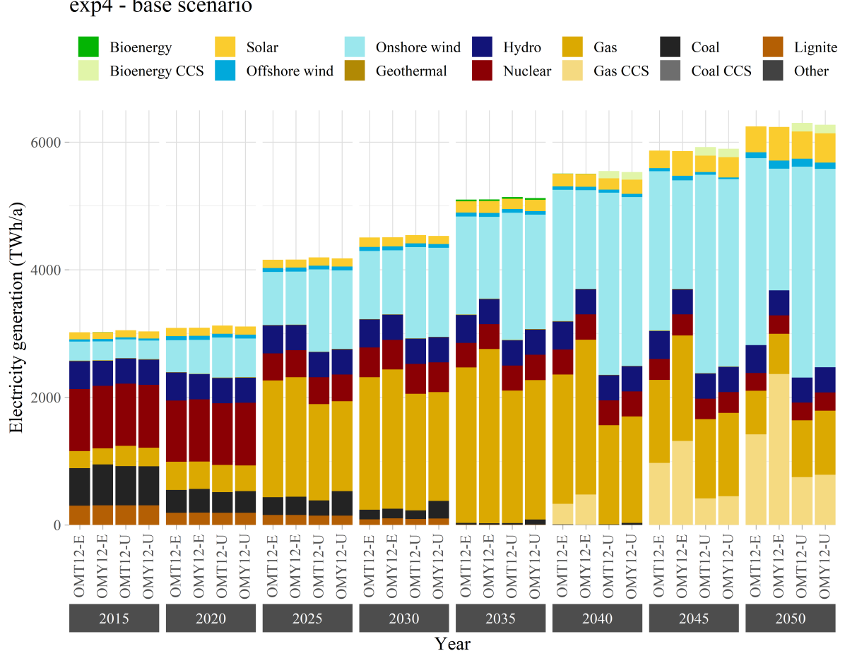
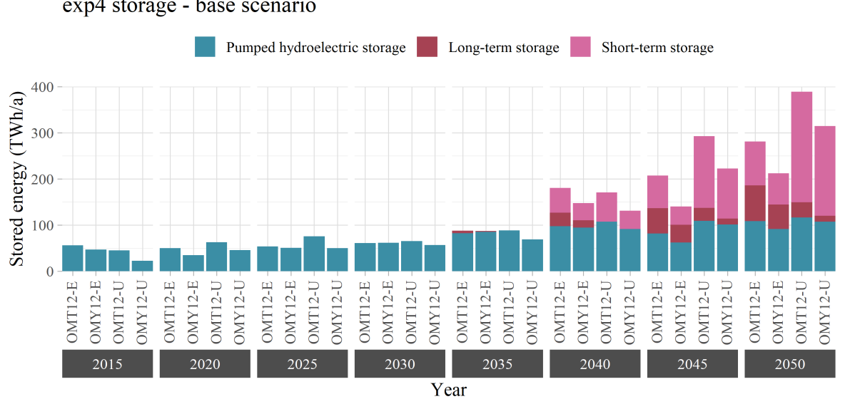
Figure 4: Electricity generation (top) and energy stored (bottom) over the period 2015-2050 for all models involved in the temporal resolution experiment.

4.5 Impact of spatial resolution

Experiment setup

Apart from the feature “spatial resolution”, all the other major features are the same. All the compared optimization models are myopic and use 384 typical time steps. They either use 28 single countries or 12 mega-regions. HECTOR is not involved in this experiment because of its inability to handle a large amount of regions. Table 7 provides an overview of the used models.

Table 7: Models used in the spatial resolution experiment.

Model variation	Optimization	Simulation	Intertemporal	Myopic	Full year	Typical steps	28 countries	12 mega-regions	Model framework
OMT28-D	X			X		X	X		DIMENSION
OMT12-D	X			X		X		X	DIMENSION
OMT28-R	X			X		X	X		EUREGEN
OMT12-R	X			X		X		X	EUREGEN
OMT28-E	X			X		X	X		E2M2
OMT12-E	X			X		X		X	E2M2
OMT28-U	X			X		X	X		urbs
OMT12-U	X			X		X		X	urbs

Results

Due to the large number of models involved in this experiment, the results regarding the energy mix were aggregated in Figure 5 for each pair of similar models. The difference between the two models for each framework is shown, meaning that positive values stand for a higher electricity generation using the depicted technologies in the models with 28 regions, while values below zero indicate that the generation in the models with 12 regions is higher. Up until 2035 (for E2M2) or 2040 (for the rest), the energy mix is characterized by an over-estimation of onshore wind generation in models with 12 regions. In models with a higher spatial resolution, this is replaced by gas, coal, nuclear, and solar. In the long term, models with 28 regions rely more on onshore wind and less on offshore wind, gas CCS, and bioenergy CCS. In absolute terms, the discrepancies could reach up to 370 TWh in 2035, which is about 7% of the energy demand of that year.

Similarly to the previous experiment, the the spatial aggregation deals with the weather data and the load separately, so that the spatial and temporal correlation between weather and load events is not preserved, which could partly explain the discrepancies. However, unlike the reduction of the temporal complexity, the spatial reduction does not preserve the full load hours of renewable generation either. In fact, when grouping two or more regions, the distribution of the potentials shifts, and the locations of the representative sites (e.g. median, upper 10%) also change. This results in completely different time series for the aggregated regions, both in shape (hourly fluctuations) and in sum (yearly full load hours). The weighting of the time series calibrates the wind and solar generation to historical data, but does not constrain future expansion. In most cases, this has led to an over-estimation of the wind potential in very large regions. Also, in the absence of transmission constraints between the countries making up each mega-region, the integration of wind is facilitated. This explains why the models with 12 regions tend to have more onshore and offshore wind. By 2040, the potential for good wind sites is already exhausted in most 12-region models. Meanwhile, the models with 28 regions profit from the existence of more efficient wind turbines to decarbonize faster, hence their higher onshore wind generation in the long term.

Sensitivity to other scenarios

Increasing the net transfer capacities makes it easier to integrate renewable energy generation from solar and onshore wind (and nuclear power, in the case of OMT12-R). Since models with a higher spatial resolution have more constraints on inter-regional trade, they usually benefit more from higher transfer capacities, which ease such constraints. EUREGEN generates more onshore wind in the high resolution model, but not any extra nuclear energy, such that it benefits less from the increased NTCs overall.

Key messages

The impact of the spatial resolution depends on the quality of the spatial aggregation of time series and transmission capacities. In this experiment, fewer regions led to more onshore and offshore generation. Easing the transmission constraints by increasing the net transfer capacities exogenously favored onshore wind, particularly in the high resolution models. The experiment echoes the recommendations of Hess et al. [38] regarding the modeling of the grid.

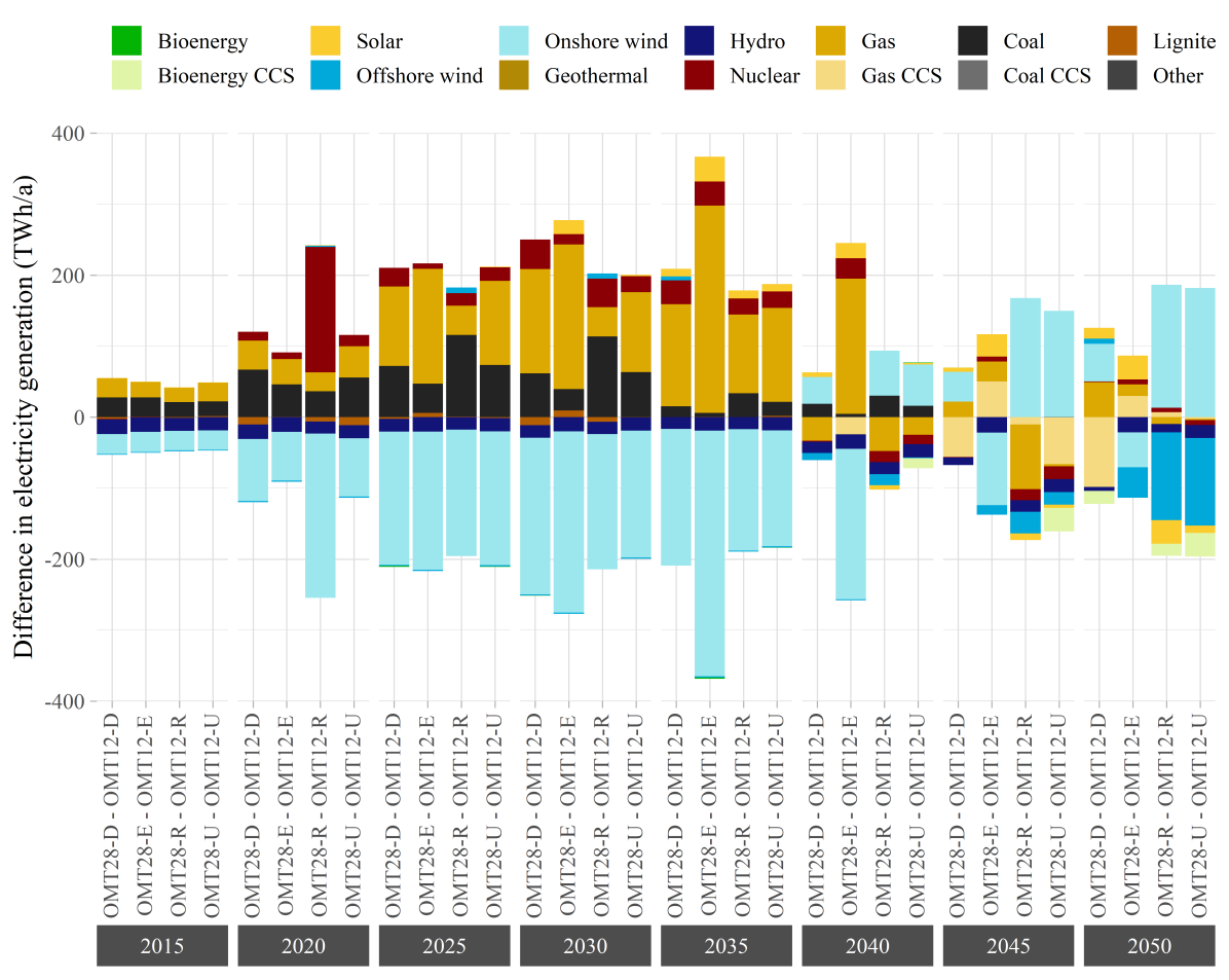
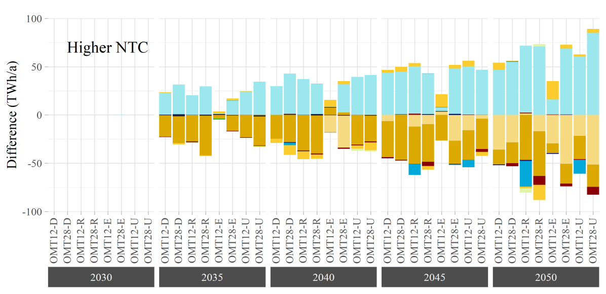
Figure 5: Difference in electricity generation between models with 28 and 12 regions over the period 2015-2050 (top) and difference due to increased net transfer capacities beyond 2030 (bottom) for all pairs of models involved in the spatial resolution experiment.

5 Conclusion and discussion

This paper assesses the impact of four major model features (model type, planning horizon, temporal resolution, spatial resolution) on the results of power market models. It uses five frameworks (DIMENSION, EUREGEN, E2M2, urbs, and HECTOR) for a qualitative and quantitative comparison. A high level of harmonization is ensured by using a joint input database and stripping the model frameworks from some of their specific features. A series of experiments is designed so that the impact of each major model feature is inspected separately. A combination of intramodel and intermodel comparisons is used in order to attribute deviations in results to the major feature analyzed.

Thanks to the high level of data and feature harmonization, clear conclusions on the behavior of the involved models could be derived from the experiments, in line with the initial objective. These conclusions are then translated into recommendations for modelers on how to minimize the discrepancies. The first finding relates to the choice of model type (optimization or simulation), which for the used models and setup leads to fundamental differences in the fleet of technologies. One possible recommendation is to use the differences synergetically through model coupling: Simulation models can build upon the results of an optimization to reduce the number of sensitivity iterations and answer specific questions that cannot be analyzed within an optimization framework. Second, in the experiment on the planning horizon (intertemporal or myopic), the choice of the appropriate configuration depends on the underlying assumptions about future developments of prices and technologies. If the scenario constraints already put the system on a decarbonization pathway, myopic models could deliver similar results to intertemporal ones, without lock-in effects. In such a case, it is recommended to use the myopic models, which are less computationally intensive. Third, the experiments on the temporal resolution (8760 or 384 time steps) and the spatial resolution (28 countries or 12 mega-regions) reveal how sensitive the models are to the input data. The choice of the aggregation method of the time steps and/or model regions has an impact on the model results. In order to improve their robustness, models need to take into account the behavior of storage in non-consecutive time periods and to reflect grid bottlenecks within the regions. Otherwise, they risk overestimating the ease of integrating renewable energy, particularly seasonal wind generation. If the future energy systems contain large amounts of fluctuating energy sources, it is recommended to use high temporal and spatial resolutions to reflect the system’s behavior and interdependencies correctly.

Even though similarity is expected in experiments with a high level of harmonization, it triggers a discussion on whether there is a need for a high number of energy system models, particularly from the perspective of funding institutions. This paper provides two arguments in favor of model plurality. First, a variety of modeling approaches allows to evaluate the bandwidth of outcomes due to model uncertainty, as done by Gillingham et al. [39]. For considering the bandwidth of power system modeling, including more than one simulation model or other model types is desirable. Second, while the results are similar within this paper, model specialties that could drive results apart from each other were not included.

This analysis comes with caveats. Only one simulation model is included in our sample and only limited conclusion can be drawn out of that. A larger sample of simulation models would allow for additional insights. The possibility of overlapping optimization as balance between myopic and intertemporal planning horizons is also neglected. Regarding the model complexity reduction techniques, the role of different levels of technology richness is not analyzed. The focus was not on the algorithms for the selection (and weighting) of typical time steps, nor for clustering regions. These aspects could be addressed in future work. The models were also not compared based on their CPU or RAM usage. Using the same computer architecture for such a comparison would provide useful insights from the software perspective. Despite all the limitations, this paper could achieve the objectives within its scope and sets a higher harmonization standard for future model comparisons.

Contributions and Acknowledgements

This work was funded by the Federal Ministry for Economic Affairs and Energy of Germany (BMWi) within the project Research Network for the Development of New Methods in Energy System Modeling (4NEMO) under grant number 0324008A. The authors would like to thank Wolfgang Habla, Kristina Govorukha, Philip Mayer and Paul Kunz for developing and providing the used scenarios. The contribution of Christoph Weissbart, Wolfgang Habla and Frieder Borggrefe in collecting information and building the input database is gratefully acknowledged.

CRediT author statement

Kais Siala: Conceptualization, Investigation, Data curation, Writing - Original Draft, Visualization; Mathias Mier: Conceptualization, Methodology, Investigation, Data curation, Writing - Original Draft; Lukas Schmidt: Conceptualization, Methodology, Investigation, Writing - Original Draft; Laura Torralba-Díaz: Methodology, Investigation, Writing - Original Draft; Siamak Sheykhha: Investigation, Writing - Original Draft; Georgios Savvidis: Methodology, Investigation, Visualization.

Appendix A Numerical assumptions

Table 1: Range of fixed operation and maintenance costs of generation technologies for all vintages.

Technologies	Fixed O&M costs [EUR2015/kW/a]
Nuclear	264
Lignite	66
Coal	55 – 60
Coal CCS	99 – 109
Gas CCGT	34
Gas ST	34
Gas OCGT	17
Gas CCS	32
OilOther	33
Bioenergy	197 – 212
Bio CCS	121 – 130
Geothermal	440 – 495
PV	8 – 15
Wind Onshore	0
Wind Offshore	76 – 131
Pumped Hydro	5.3
Short-Term Storage	6.6 – 21.1
Long-Term Storage	30.4

Table 2: Full-load efficiency [%] of generation technologies for vintage classes based on their commissioning year.

Technologies	1965	1970	1975	1980	1985	1990	1995	2000	2005
Bioenergy	-	-	-	-	-	20.0	20.0	20.0	20.0
Bio CCS	-	-	-	-	-	-	-	-	-
Coal	33.0	33.0	34.2	35.5	36.2	37.0	38.5	40.0	41.5
Coal CCS	-	-	-	-	-	-	-	-	-
Gas CCGT	40.0	40.0	41.0	42.0	46.1	50.0	52.6	54.9	56.5
Gas OCGT	23.0	23.0	25.0	27.0	29.5	32.1	34.5	37.0	38.3
Gas ST	40.0	40.0	41.0	42.0	46.1	50.0	52.6	54.9	56.5
Gas CCS	-	-	-	-	-	-	-	-	-
Lignite	35.0	35.0	36.0	37.0	37.5	38.0	40.5	42.9	44.4
Nuclear	40.0	40.0	41.0	42.0	46.1	50.0	52.6	54.9	56.5
OilOther	30.9	30.9	30.9	30.9	30.9	30.9	30.9	30.9	30.9
Pumped Hydro	79.2	79.2	79.2	79.2	79.2	79.2	79.2	79.2	79.2
Short-Term Storage	-	-	-	-	-	-	-	-	-
Long-Term Storage	-	-	-	-	-	-	-	-	-
Technologies	2010	2015	2020	2025	2030	2035	2040	2045	2050
Bioenergy	20.0	20.0	20.4	20.9	21.3	21.3	22.1	22.1	23.0
Bio CCS	-	20.0	20.0	20.0	20.0	20.0	20.0	20.0	20.0
Coal	42.9	44.8	46.8	48.0	49.1	49.1	49.1	49.1	49.1
Coal CCS	-	44.9	44.9	44.9	44.9	44.9	44.9	44.9	44.9
Gas CCGT	58.1	59.2	60.1	61.1	62.1	62.1	62.1	62.1	62.1
Gas OCGT	39.5	41.7	43.6	44.5	45.5	46.0	46.5	46.5	46.5
Gas ST	58.1	59.2	60.1	61.1	62.1	62.1	62.1	62.1	62.1
Gas CCS	-	59.1	59.1	59.1	59.1	59.1	59.1	59.1	59.1
Lignite	45.9	47.8	-	-	-	-	-	-	-
Nuclear	58.1	59.2	60.1	61.1	62.1	62.1	62.1	62.1	62.1
OilOther	30.9	30.9	-	-	-	-	-	-	-
Pumped Hydro	79.2	79.2	79.2	79.2	79.2	79.2	79.2	79.2	79.2
Short-Term Storage	-	90.0	90.0	90.0	90.0	90.0	90.0	90.0	90.0
Long-Term Storage	-	36.0	36.0	36.0	36.0	36.0	36.0	36.0	36.0

Table 3: Development of carbon prices [EUR₂₀₁₅/t].

Scenario	2015	2020	2025	2030	2035	2040	2045	2050
Base	7.8	15.0	22.0	27.0	56.0	68.0	102.0	132.0
Lower CO2 price	7.8	15.0	18.0	19.0	34.0	34.0	42.0	44.0
Higher CO2 price	7.8	15.0	23.0	31.0	68.0	85.0	132.0	176.0

Table 4: Development of investment costs [EUR₂₀₁₅/kW].

Technology	2015	2020	2025	2030	2035	2040	2045	2050
Nuclear	6600	6006	5346	5082	4818	4488	4488	4356
Lignite	1640	1640	1640	1640	1640	1640	1640	1640
Coal	1500	1500	1440	1410	1395	1380	1380	1365
Coal CCS	3415	3415	3278	3210	3176	3142	3142	3108
Gas CCGT	850	850	850	850	850	850	850	850
Gas ST	850	850	850	850	850	850	850	850
Gas OCGT	437	437	437	437	437	437	437	437
Gas CCS	1495	1495	1495	1495	1495	1495	1495	1495
OilOther	822	822	822	822	822	822	822	822
Bioenergy	4322	4236	4149	4149	4106	4063	4063	4020
Bioenergy CCS	4450	4361	4272	4272	4228	4183	4183	4139
Geothermal	12364	11993	11622	11498	11251	11127	11004	11004
PV	1300	1027	936	858	819	780	741	715
Onshore wind	1520	1397	1368	1339	1325	1310	1310	1296
Offshore wind	3600	3024	2700	2520	2376	2268	2160	2088
Short-term storage	1740	1740	1440	1120	1120	780	780	440
Long-term storage	1520	1520	1520	1520	1520	1520	1520	1520

Table 5: Development of fuel prices [EUR₂₀₁₅/MWh_th].

Fuel	2015	2020	2025	2030	2035	2040	2045	2050
Uranium	2.3	2.3	2.3	2.3	2.3	2.3	2.3	2.3
Lignite	7.0	7.0	7.0	7.0	7.0	7.0	7.0	7.0
Coal	8.3	8.2	8.1	7.9	7.8	7.7	7.6	7.5
Natural gas	20.7	20.3	20.0	19.7	19.3	19.0	18.8	18.5
Oil	40.3	40.8	41	41.2	41.4	41.8	42.3	42.6
Bioenergy	12.0	12.0	12.0	12.0	12.0	12.0	12.0	12.0

Table 6: Development of electricity demand [TWh/a].

Country	2015	2020	2025	2030	2035	2040	2045	2050
AT	63.5	64.3	78.3	91.1	137.1	146.9	155.5	163.0
BE	83.1	82.2	96.6	107.3	131.5	158.0	181.6	196.2
BG	29.6	30.1	34.7	36.0	37.3	40.4	42.7	44.4
CH	58.2	60.8	67.2	70.5	116.3	126.0	136.3	147.5
CZ	58.7	62.6	116.8	122.9	126.8	135.2	144.8	153.7
DE	528.1	533.9	832.3	842.8	844.9	874.3	908.5	946.0
DK	31.8	31.8	36.6	35.1	39.3	46.8	52.1	55.4
EE	7.4	7.6	9.3	11.4	11.6	12.2	12.7	13.3
EL	52.4	52.8	58.0	54.9	58.8	64.2	69.6	73.4
ES	238.6	247.5	312.7	367.0	493.1	522.4	542.2	566.9
FI	79.7	72.6	82.9	79.2	80.0	82.1	87.3	90.9
FR	447.7	449.9	759.0	766.8	811.5	864.3	922.3	980.0
HR	15.7	15.7	17.4	17.6	18.2	20.4	23.0	25.4
HU	38.1	36.7	44.2	52.9	67.5	71.4	75.4	82.0
IE	25.7	26.1	30.6	32.6	39.3	42.5	45.1	49.1
IT	297.2	318.7	421.4	564.1	599.8	648.7	694.2	739.9
LT	10.2	12.1	18.4	18.1	17.2	17.8	18.9	19.8
LU	6.2	6.5	7.4	8.2	11.6	14.2	15.5	17.3
LV	6.5	6.6	7.7	8.6	10.0	11.8	12.4	12.9
NL	109.4	113.3	148.9	186.9	191.9	202.3	213.5	230.1
NO	119.3	124.0	130.3	124.9	157.0	166.8	176.8	187.6
PL	138.9	143.3	164.3	180.2	231.1	269.1	281.6	293.7
PT	46.9	51.8	60.9	62.1	66.2	70.2	73.5	76.2
RO	46.9	47.0	54.2	57.6	59.9	66.3	73.6	79.3
SE	127.8	132.8	158.5	161.1	232.7	250.4	268.6	287.8
SI	12.9	13.1	15.3	16.6	19.4	21.5	22.8	24.1
SK	25.4	26.7	33.5	39.1	48.1	56.7	58.7	61.0
UK	311.2	317.1	358.1	388.1	433.5	484.7	527.9	588.7

Appendix B Conducted runs

The outputs for all model runs (data and plots) as well as the scripts for plotting are shared with open licenses in this repository for supplementary materials [36].

Table 1: Overview of all the conducted model runs.

Model framework	Model variation	Optimization	Simulation	Intertemporal	Myopic	Full year	Typical steps	28 countries	12 mega-regions	base	higher CO2 price	lower CO2 price	increased NTC
DIMENSION	OIT28-D	X		X			X	X		X	X	X	X
	OIT12-D	X		X			X		X	X	X	X	X
	OMT28-D	X			X		X	X		X	X	X	X
	OMT12-D	X			X		X		X	X	X	X	X
EUREGEN	OIT12-R	X		X			X		X	X	X	X	X
	OMT28-R	X			X		X	X		X	X	X	X
	OMT12-R	X			X		X		X	X	X	X	X
E2M2	OMY12-E	X			X	X			X	X
	OMT28-E	X			X		X	X		X	X	X	X
	OMT12-E	X			X		X		X	X	X	X	X
urbs	OMY28-U	X			X	X		X		X
	OMY12-U	X			X	X			X	X
	OMT28-U	X			X		X	X		X	X	X	X
	OMT12-U	X			X		X		X	X	X	X	X
HECTOR	SMT12-H		X		X		(X)		X	X	X	X	X

References

- Mier and Weissbart [2020] M. Mier, C. Weissbart, Power markets in transition: Decarbonization, energy efficiency, and short-term demand response, Energy Economics 86 (2020) 104644.
- Helgeson and Jakob [2020] B. Helgeson, P. Jakob, The role of electricity in decarbonizing European road transport – Development and assessment of an integrated multi-sectoral model, Applied Energy 262 (2020) 114365.
- Pfenninger et al. [2014] S. Pfenninger, A. Hawkes, J. Keirstead, Energy systems modeling for twenty-first century energy challenges, Renewable and Sustainable Energy Reviews 33 (2014) 74–86.
- Gacitua et al. [2018] L. Gacitua, P. Gallegos, R. Henriquez-Auba, A. Lorca, M. Negrete-Pincetic, D. Olivares, A. Valenzuela, G. Wenzel, A comprehensive review on expansion planning: Models and tools for energy policy analysis, Renewable and Sustainable Energy Reviews 98 (2018) 346–360.
- Hall and Buckley [2016] L. M. Hall, A. R. Buckley, A review of energy systems models in the UK: Prevalent usage and categorisation, Applied Energy 169 (2016) 607–628.
- Connolly et al. [2010] D. Connolly, H. Lund, B. V. Mathiesen, M. Leahy, A review of computer tools for analysing the integration of renewable energy into various energy systems, Applied Energy 87 (2010) 1059–1082.
- Savvidis et al. [2019] G. Savvidis, K. Siala, C. Weissbart, L. Schmidt, F. Borggrefe, S. Kumar, K. Pittel, R. Madlener, K. Hufendiek, The gap between energy policy challenges and model capabilities, Energy Policy 125 (2019) 503–520.
- Ommen et al. [2014] T. Ommen, W. B. Markussen, B. Elmegaard, Comparison of linear, mixed integer and non-linear programming methods in energy system dispatch modelling, Energy 74 (2014) 109–118.
- Pfenninger [2017] S. Pfenninger, Dealing with multiple decades of hourly wind and PV time series in energy models: A comparison of methods to reduce time resolution and the planning implications of inter-annual variability, Applied Energy 197 (2017) 1–13.
- Nahmacher et al. [2016] P. Nahmacher, E. Schmid, L. Hirth, B. Knopf, Carpe Diem: A Novel Approach to Select Representative Days for Long-Term Power System Models with High Shares of Renewable Energy Sources, Energy 112 (2016) 430–442.
- Frew and Jacobson [2016] B. A. Frew, M. Z. Jacobson, Temporal and spatial tradeoffs in power system modeling with assumptions about storage: An application of the power model, Energy 117 (2016) 198–213.
- Priesmann et al. [2019] J. Priesmann, L. Nolting, A. Praktiknjo, Are complex energy system models more accurate? An intra-model comparison of power system optimization models, Applied Energy 255 (2019) 113783.
- Diaz et al. [2019] G. Diaz, A. Inzunza, R. Moreno, The importance of time resolution, operational flexibility and risk aversion in quantifying the value of energy storage in long-term energy planning studies, Renewable and Sustainable Energy Reviews 112 (2019) 797–812.
- Van Vuuren et al. [2009] D. P. Van Vuuren, M. Hoogwijk, T. Barker, K. Riahi, S. Boeters, J. Chateau, S. Scrieciu, J. van Vliet, T. Masui, K. Blok, et al., Comparison of top-down and bottom-up estimates of sectoral and regional greenhouse gas emission reduction potentials, Energy Policy 37 (2009) 5125–5139.
- Capros et al. [2014] P. Capros, L. Paroussos, P. Fragkos, S. Tsani, B. Boitier, F. Wagner, S. Busch, G. Resch, M. Blesl, J. Bollen, European decarbonisation pathways under alternative technological and policy choices: A multi-model analysis, Energy Strategy Reviews 2 (2014) 231–245.
- Förster et al. [2013] H. Förster, K. Schumacher, E. De Cian, M. Hübler, I. Keppo, S. Mima, R. D. Sands, European energy efficiency and decarbonization strategies beyond 2030—a sectoral multi-model decomposition, Climate Change Economics 4 (2013) 1340004.
- Knopf et al. [2013] B. Knopf, Y.-H. H. Chen, E. De Cian, H. Förster, A. Kanudia, I. Karkatsouli, I. Keppo, T. Koljonen, K. Schumacher, D. P. Van Vuuren, Beyond 2020—Strategies and costs for transforming the European energy system, Climate Change Economics 4 (2013) 1340001.
- Deane et al. [2012] J. Deane, A. Chiodi, M. Gargiulo, B. P. Ó. Gallachóir, Soft-linking of a power systems model to an energy systems model, Energy 42 (2012) 303–312.
- Kiviluoma et al. [2018] J. Kiviluoma, E. Rinne, N. Helistö, Comparison of flexibility options to improve the value of variable power generation, International Journal of Sustainable Energy 37 (2018) 761–781.
- Poncelet et al. [2016] K. Poncelet, E. Delarue, D. Six, J. Duerinck, W. D’haeseleer, Impact of the level of temporal and operational detail in energy-system planning models, Applied Energy 162 (2016) 631–643.
- Gils et al. [2019] H. C. Gils, T. Pregger, F. Flachsbarth, M. Jentsch, C. Dierstein, Comparison of spatially and temporally resolved energy system models with a focus on Germany’s future power supply, Applied Energy 255 (2019) 113889.
- Richter [2011] J. Richter, DIMENSION - A Dispatch and Investment Model for European Electricity Markets, EWI Working Paper 11/03 (2011).
- Weissbart and Blanford [2019] C. Weissbart, G. J. Blanford, A framework for modeling the dynamics of power markets-The EU-REGEN model, ifo Working Papers No. 307 (2019).
- Sun [2013] N. Sun, Modellgestützte Untersuchung des Elektrizitätsmarktes: Kraftwerkseinsatzplanung und -Investitionen, Ph.d. thesis, Institute of Energy Economics and Rational Energy Use, University of Stuttgart, 2013.
- Dorfner et al. [2018] J. Dorfner, M. Dorfner, K. Schönleber, S. Candas, smuellr, D. Üzrek, wyaudi, Y. Özsahin, adeeljsid, T. Zipperle, S. Herzog, L. Odersky, K. Siala, O. Akca, urbs: v0.7.3: A linear optimisation model for distributed energy systems, Chair of Renewable and Sustainable Energy Systems, Technical University of Munich, 2018. Doi: 10.5281/zenodo.1228851.
- Sheykhha and Madlener [2019] S. Sheykhha, R. Madlener, HECTOR – A Dynamic Dispatch and Investment Model for Electricity Markets in Europe, FCN Working Paper No. 23/2019, Institute for Future Energy Consumer Needs and Behavior, RWTH Aachen University, 2019.
- Mier et al. [2020] M. Mier, K. Siala, K. Govorukha, P. Mayer, Costs and benefits of political and physical collaboration in the European Power Market, ifo Working Paper 343, ifo Institute - Leibniz Institute for Economic Research at the University of Munich, Munich, 2020.
- Weimer-Jehle [2006] W. Weimer-Jehle, Cross-impact balances: A system-theoretical approach to cross-impact analysis, Technological Forecasting and Social Change 73 (2006) 334–361.
- Böhringer et al. [2004] C. Böhringer, F. Eckermann, A. Löschel, PACE, Forum für Energiemodelle und Energiewirtschaftliche Systemanalysen in Deutschland Energiemodelle zum Klimaschutz in liberalisierten Energiemärkten, Die Rolle erneuerbarer Energieträger, Umwelt- und Ressourcenökonomik, Bd. 21 59 (2004) 123–136.
- European Commission [2020] European Commission, Commission Staff Working Document SWD/2020/176: Impact Assessment on Stepping up Europe’s 2030 climate ambition Investing in a climate-neutral future for the benefit of our people, Technical Report, European Commission, 2020.
- European Commission [2018] European Commission, Communication com(2018) 77: In-depth analysis in support of the commission 3 - A Clean Planet for all. A European long-term strategic vision for a prosperous, modern, competitive and climate neutral economy, Technical Report, European Commission, 2018.
- Siala and Houmy [2020] K. Siala, H. Houmy, tum-ens/pyGRETA: python Generator of REnewable Time series and mAps (Version v1.0.1)., 2020.
- Gils et al. [2021] H. C. Gils, H. Gardian, M. Kittel, W.-P. Schill, A. Zerrahn, A. Murmann, J. Launer, A. Fehler, F. Gaumnitz, J. van Ouwerkerk, et al., Modeling flexibility in energy systems – comparison of power sector models based on simplified test cases, Renewable and Sustainable Energy Reviews (2021).
- Ramachandran et al. [2021] S. Ramachandran, K. Siala, C. de la Rua, T. Massier, A. Ahmed, T. Hamacher, Life cycle impacts of a cost-optimal HVDC connection to import solar energy from Australia to Singapore, energies 14 (2021) 7178.
- Bertsch et al. [2016] J. Bertsch, C. Growitsch, S. Lorenczik, S. Nagl, Flexibility in europe’s power sector—an additional requirement or an automatic complement?, Energy Economics 53 (2016) 118–131.
- Siala et al. [2020] K. Siala, M. Mier, L. Schmidt, L. Torralba-Díaz, S. Sheykhha, G. Savvidis, Supplementary materials for manuscript "Which model features matter? An experimental approach to evaluate power market modeling choices", 2020. Doi: 10.5281/zenodo.4120576.
- Heuberger et al. [2017] C. F. Heuberger, E. S. Rubin, I. Staffell, N. Shah, N. Mac Dowell, Power capacity expansion planning considering endogenous technology cost learning, Applied Energy 204 (2017) 831–845.
- Hess et al. [2018] D. Hess, M. Wetzel, K.-K. Cao, Representing node-internal transmission and distribution grids in energy system models, Renewable Energy 119 (2018) 874–890.
- Gillingham et al. [2015] K. Gillingham, W. D. Nordhaus, D. Anthoff, G. Blanford, V. Bosetti, P. Christensen, H. McJeon, J. Reilly, P. Sztorc, Modeling uncertainty in climate change: A multi-model comparison, NBER Working Paper No. 21637 (2015).