Deep generative LDA

Abstract

Linear discriminant analysis (LDA) is a popular tool for classification and dimension reduction. Limited by its linear form and the underlying Gaussian assumption, however, LDA is not applicable in situations where the data distribution is complex. Recently, we proposed a discriminative normalization flow (DNF) model. In this study, we reinterpret DNF as a deep generative LDA model, and study its properties in representing complex data. We conducted a simulation experiment and a speaker recognition experiment. The results show that DNF and its subspace version are much more powerful than the conventional LDA in modeling complex data and retrieving low-dimensional representations.

Index Terms—  Linear discriminant analysis; Normalization flow; Deep generative model; Dimension reduction

1 Introduction

Linear discriminant analysis (LDA), sometimes called Fisher discriminant analysis (FDA), was first proposed by Fisher in 1936 [1] and is a classic tool for dimension reduction. Although the original form is purely discriminative, Campbell et al. [2] showed that LDA corresponds to a linear Gaussian model, where each class is represented by a Gaussian distribution, and different classes share the same covariance matrix. This model is purely generative and is trained by maximum likelihood (ML). By this generative model view, LDA is regarded as a general model for discrimination tasks, and dimension reduction is just a by-product and can be derived by constraining the class means in a subspace [2].

In spite of the wide application, blindly employing LDA may suffer from serious problems if the data is not distributed as homogeneous (covariance-shared) Gaussians, e.g., the small sample size (SSS) problem [3, 4], non-linearly separate problem [3, 5], and heteroscedasticity and non-Gaussianity problem [2, 6, 7]. In order to handle complex data, the homogeneous Gaussian assumption has to be relaxed. To mention several, the quadratic discriminant analysis (QDA) [8] and the heteroscedastic LDA (HLDA) [7] relax the shared-covariance assumption; the mixture discriminant analysis (MDA) [9] relaxes the Gaussian assumption by allowing data to distribute as a Gaussian mixture; the kernel discriminant analysis [10] relaxes the Gaussian assumption by introducing a non-linear transformation. The above extensions (and other alternatives) can deal with non-Gaussian and non-homogeneous data, but their learning capacity is often constrained by their model forms and so cannot represent general data. Moreover, some of the extensions are only applicable for discrimination tasks, but not for dimension reduction, e.g., QDA [8].

Deep neural networks (DNN) have shown remarkable power in learning abstract features from complex data [11]. From the perspective of dimension reduction, DNN can perform this task extremely well by compressing class information into a short feature vector, by performing discriminative training with the cross-entropy objective, or an objective that is exactly the same as LDA, the Fisher criterion [12]. However, the features derived by the discriminative training will not gain any simple form of distribution, and generally lose their capacity of explaining the data.

Recently, we proposed a discriminative normalization flow (DNF) model and used it to normalize class distributions [13]. In this paper, we reinterpret DNF as a nonlinear extension of LDA. Compared to the early work such as QDA and MDA, the new model is based on deep neural networks and so inherits their brilliant power in learning from data, which grants DNF the capacity of modeling any kind of data in theory. Compared to other ‘deep LDA’ models that are based on DNNs, our model is generative and can explain the data by generation. Most importantly, our model holds the homogeneous Gaussian assumption in the latent space, and can be trained by maximum likelihood. All of these features make it highly resemble the conventional LDA, except that the linear transformation is replaced by a neural networks. When the DNN is implemented as a linear transformation, the model falls back to the standard LDA. Due to such resemblance, DNF can be interpreted as deep generative LDA, to emphasize its deep nature and discriminate it from other ‘deep LDAs’ based on discriminative training [12]. Fig. 1 compares the LDA and DNF.

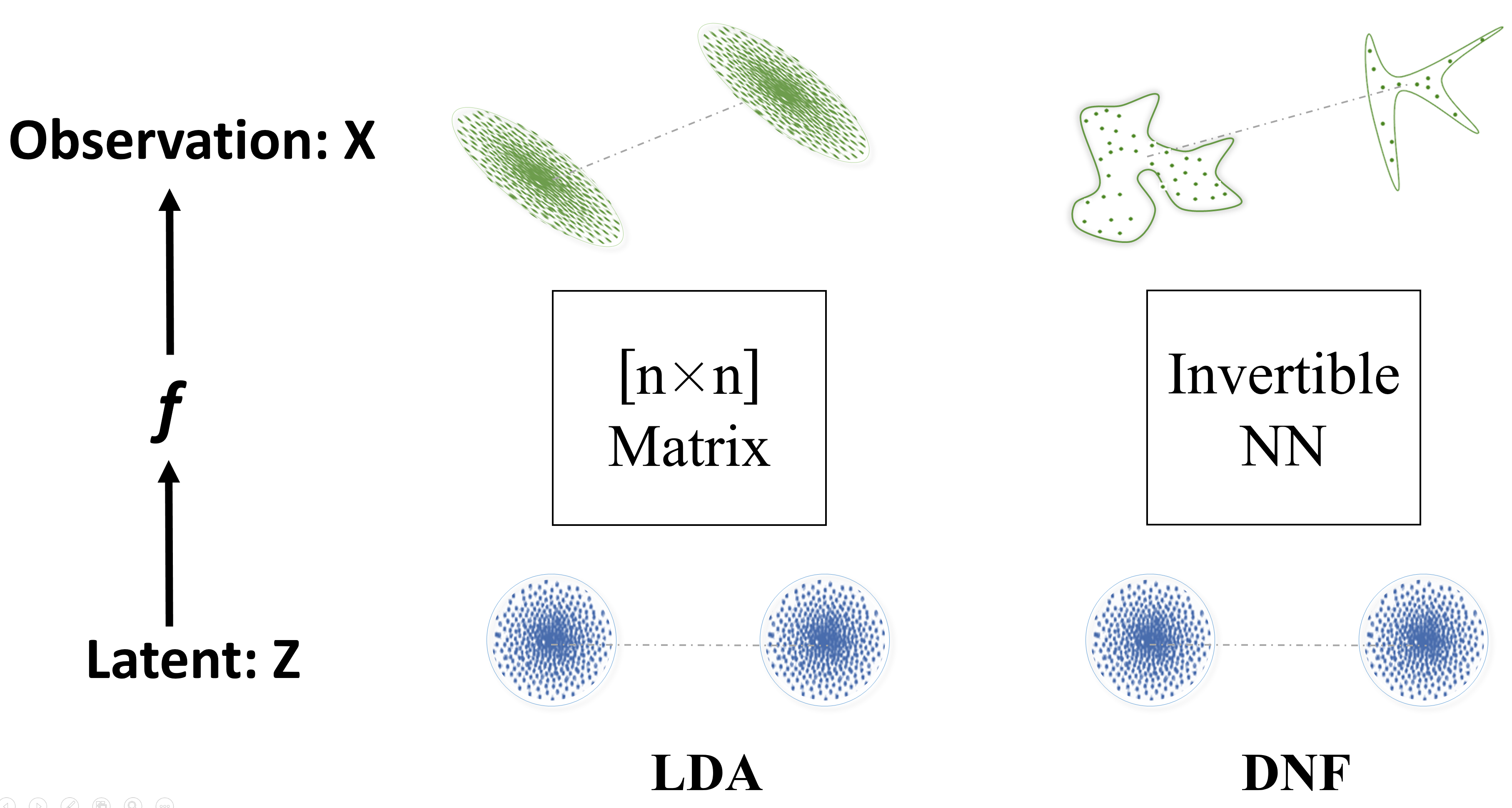
Fig. 1: (Left) LDA maps standard Gaussians to homogeneous Gaussians by a linear transformation; (Right) DNF maps standard Gaussians to heterogeneous distributions in complex forms.

2 Deep LDA by Discriminative Normalization Flow

2.1 Probabilistic view of LDA

LDA can be cast to a linear Gaussian model [2], where each class is a Gaussian and all classes share the same covariance, as formulated below:

$$p(\mathbf{x};y(\mathbf{x}))=N(\mathbf{x};\boldsymbol{\nu}_{y(\mathbf{x})},\boldsymbol{\Sigma}).$$ (1)

Define an invertible linear transformation $\mathbf{z}=\mathbf{M}\mathbf{x}$ that projects the observation $\mathbf{x}$ to a latent code $\mathbf{z}$, for which each class is a standard Gaussian.

$$p(\mathbf{z};y(\mathbf{x}))=N(\mathbf{z};\boldsymbol{\mu}_{y(\mathbf{x})},\boldsymbol{I}),$$ (2)

The probability $p(\mathbf{x})$ and the probability $p(\mathbf{z})$ has the following relation:

$$p(\mathbf{x};y(\mathbf{x}))=p(\mathbf{z};y(\mathbf{x}))|\det\mathbf{M}|.$$ (3)

where $\det\mathbf{M}$ represents determinant of $\mathbf{M}$. Given a set of training data $\{\mathbf{x}_{i}\}$, the likelihood of the data can be computed as follows:

$$L(\mathbf{M}) = \sum_{i}\log(p(\mathbf{x}_{i};y(\mathbf{x}_{i})))$$ (4)

$$= \sum_{i}\big{\{}\log(p(\mathbf{z}_{i};y(\mathbf{x}_{i})))+\log|\det\mathbf{M}|\big{\}}$$ (5)

Maximizing $L(\mathbf{M})$ with respect to $\mathbf{M}$ leads to the full-dimension LDA.

As shown by Kumar et al. [7], LDA-based dimension reduction can be derived by constraining the class means in a low-dimensional subspace. For that purpose, one can assume that only part of the dimensions of the class means in the latent space are class-dependent, as shown below:

$$\boldsymbol{\mu}_{y}=\begin{bmatrix}\boldsymbol{\mu}_{y}^{c}\\ \boldsymbol{\mu}^{0}\end{bmatrix},$$ (6)

where $\boldsymbol{\mu}_{y}^{c}$ is class-dependent and $\boldsymbol{\mu}^{0}_{y}$ is shared by all classes. Under this assumption, optimizing the transformation $\mathbf{M}$ via maximum likelihood leads to the dimension-reduction LDA, and the submatrix of $\mathbf{M}$ corresponding to the dimensions of $\boldsymbol{\mu}_{y}^{c}$ forms the dimension-reduced transformation.

2.2 Normalization flow

Normalization Flow (NF) is a deep generative model based on the principle of distribution transformation for continuous variables [14]. If a latent variable $\mathbf{z}$ and an observation variable $\mathbf{x}$ are linked by an invertible transformation as $\mathbf{x}=f(\mathbf{z})$, their probability densities have the following relationship:

$$p(\mathbf{x})=p(\mathbf{z})|\mathbf{J_{\mathbf{x}}}|,$$ (7)

where the first term on the right hand side is the prior probability of the latent codes, which we set to be a standard Gaussian; the second term $\mathbf{J_{\mathbf{x}}}=\det\frac{\partial f^{-1}(\mathbf{x})}{\partial\mathbf{x}}$ is the determinant of the Jacobian matrix of $f^{-1}$, often known as the entropy term. It has been shown that if $f$ is flexible enough, any complex distribution $p(\mathbf{x})$ can be transformed to a standard Gaussian [15]. Usually $f$ is implemented by a neural networks.

The NF model can be trained by maximum likehood with respect to the parameters of $f$. Given a set of training data $\{\mathbf{x}_{i}\}$, the likelihood function can be written by:

$$L(\bm{\theta})=\sum_{i}\log p(\mathbf{x}_{i})=\sum_{i}\big{\{}\log p(\mathbf{z}_{i})+\log|\mathbf{J}_{\mathbf{x}_{i}}|\big{\}},$$

where $\bm{\theta}$ denotes the parameters of the NF network. Since $p(\mathbf{z})$ is a Gaussian, the prior term in the objective can be easily computed. For the entropy term, however, a special structure design is required to ensure that the Jacobian matrix is tractable, e.g., [16, 17]. The objective function can be optimized by any numerical optimizers, e.g., stochastic gradient descent (SGD).

2.3 DNF: real deep LDA

NF is a powerful tool for normalizing complex distributions, however it does not consider any class information and therefore may lose the class structure during the projection, as shown in the top row of Fig. 2.

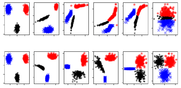
Fig. 2: Normalization process of vanilla NF (top) and DNF (bottom) with 2-dimensional data sampled from 3 Gaussian components. Vanilla NF transforms all the data to be a single Gaussian, while DNF transforms each class to an individual Gaussian.

To solve this problem, we extended NF to DNF, a discriminative normalization flow [13]. It is simply a NF but each class owns its individual class mean:

$$p(\mathbf{x};y(\mathbf{x}))=p(\mathbf{z};y(\mathbf{x}))\Bigg{|}\det\frac{\partial f^{-1}(\mathbf{x})}{\partial\mathbf{x}}\Bigg{|},$$ (8)

where $p(\mathbf{z};y(\mathbf{x}))$ is a Gaussian in the form of Eq. (2). DNF can be trained in the same fashion as NF. As shown in the bottom row of Fig. 2, DNF projection preserves the class structure.

An interesting observation is that the likelihood function in LDA (Eq.(3)) and DNF (Eq.(8)) are very similar. The only difference is on the entropy term, which is based on a linear transformation $\mathbf{x}=\mathbf{M}^{-1}\mathbf{z}$ in LDA and an invertible (may be nonlinear and complex) transformation $\mathbf{x}=f(\mathbf{z})$ in DNF. Besides the resemblance in the form of likelihood function, LDA and DNF share the same assumption that the class distributions in the latent space are homogeneous Gaussians, and the training criterion are both based on maximum likelihood. Essentially, the two models can be regarded fundamentally the same in the sense that both try to explain data by standard Gaussians. Nevertheless, the nonlinear transformation of DNF substantially extend the range of data that can be ‘explained’, especially when the transformation is materialized by deep neural networks. For example, DNF is able to deal with non-homogeneous and non-Gaussian class distributions.

2.4 Subspace DNF

Thanks to the resemblance between DNF and LDA, dimension reduction can be conducted following the same argument of Kumar [7]. Specifically, we divide the latent space into a class-dependent part and a class-independent part, as does in the dimension-reduction LDA shown in Eq.(6), and then train the DNF model as usual. By this setting, the class means are constrained in a subspace spanned by $\bm{\mu}^{c}_{y}$, so the model is called subspace DNF. Compared to dimension-reduction LDA, subspace DNF performs a nonlinear dimension reduction.

3 Related works

Researchers have tried to combine deep neural networks and LDA, and call the resultant model ‘deep LDA’. For example, Stuhlsatz et al [18] pre-trained a deep neural networks and then refined the net by Fisher discriminant criterion. The same idea motivated the work by Matthias et al. [12], where the Fisher discriminant criterion was formulated as a function of the eigenvalues of $\bm{S}_{W}^{-1}\bm{S}_{B}$, and the model was trained in an end-to-end fashion. All of them focused on the Fisher criterion superficially in order to mimic LDA, but that criterion is not necessarily better than cross entropy.

4 Simulation experiment

In this section, we compare LDA and DNF by a simulation experiment. We firstly sample 3-dimensional latent codes $\mathbf{z}$ of 4 classes, each class being an independent Gaussian. The class means span in two dimensions, and the third dimension is simply set to be zero for all the class means. We use two randomly initialized NF models to transformation $\mathbf{z}$ to $\mathbf{x}$: one is a Real NVP flow [16] with 20 blocks and the other is a MAF flow [17] with 10 blocks. The latent codes and the observations generated by the two flows are shown in the first two columns in Fig. 3. In each group of pictures, we show both the 3-D view and 2-D views from three angles. It can be seen that the distributions of the observation data generated by the two flows are rather complex.

Now we perform DNF, subspace DNF (DNF-S) and LDA to map the data $\mathbf{x}$ back to the latent codes $\mathbf{z}$, as shown in column 3-5 in Fig. 3. It is clearly to see that LDA fails to explain the data, as the latent codes do not distribute as the original 4 Gaussians. In contrast, DNF-S recovers the latent distribution almost perfectly. DNF can also find the clusters of the classes, however the class means may be scattered in the full 3-dimensional space. This is expected as there is not a subspace constraint in this model.

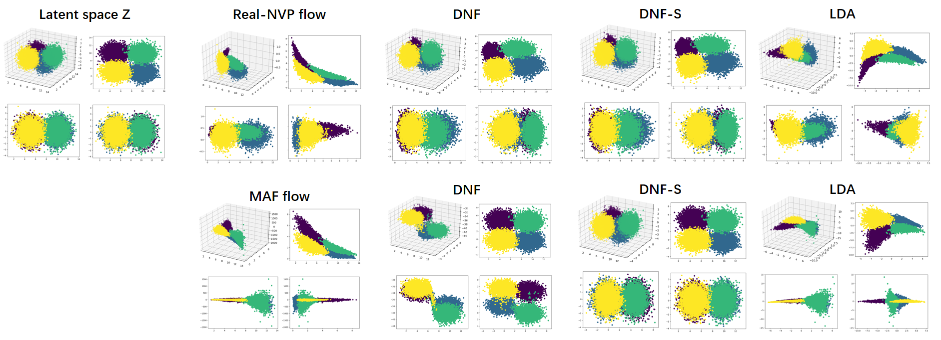
Fig. 3: 2D and 3D visualization for the simulation experiment. The first column shows the sample code $\bm{z}$; the second column shows the observation data $\mathbf{x}$ transformed from $\mathbf{z}$ by two NF models; the third to fifth columns show the recovered latent code $\mathbf{z}$ by DNF, subspace DNF and LDA, respectively.

5 Experiment on speaker recognition

Modern speaker recognition is based on deep speaker embedding to extract speaker vectors and employs PLDA [19] to score trials. In this experiment, we employ LDA and subspace DNF to perform dimension reduction for speaker vectors, in order to improve sample efficiency for the PLDA modeling.

5.1 Data and setting

Three datasets were used in our experiments: VoxCeleb [20, 21], SITW [22] and CNCeleb [23]. VoxCeleb was used to train models (x-vector, PLDA, LDA, subspace DNF), while the other two were used for performance evaluation. We use x-vector model to produce speaker vectors. The model was created using the Kaldi toolkit [24], following the SITW recipe.

We implemented the subspace DNF model with the MAF architecture [17]. It consists of 10 MAF blocks, and each block is an inverse autoregressive transformation. For more details of the MAF architecture, please refer to [17], or the code we published online. More details of the experimental system can be found in our previous work [13].

5.2 Results

Table 1: EER(%) results on SITW and CNCeleb.

Model		SITW	CNCeleb
Dimension Reduction	System [Dim]	PLDA	PLDA
N/A	x-vector [512]	5.30	13.03
Linear	LDA [512]	5.30	13.03
	LDA [400]	4.65	12.28
	LDA [200]	3.96	13.50
	LDA [150]	4.07	14.37
Nonlinear	DNF-S [512]	3.66	11.82
	DNF-S [400]	3.53	11.66
	DNF-S [150]	4.62	12.83

Table 1 shows the results in terms of Equal Error Rate (EER). Firstly notice that on SITW, which is mostly an in-domain test, both LDA and subspace DNF achieve substantial performance improvement, compared to the original x-vector system. For LDA, the best performance is obtained when the dimension is reduced to 200. For subspace DNF, we can only reduce the dimension to 400, and most performance improvement is not due to dimension reduction, but the nonlinear normalization provided by the full-dimension DNF [13]. Nonetheless, the results show that a nonlinear dimension reduction can be achieved by subspace DNF, and it may lead to additional performance gain over nonlinear normalization. On CNCeleb, which is an out-of-domain test, subspace DNF shows more advantage, demonstrating its better generalization capability.

Fig. 4 shows the latent space corresponding to class-dependent dimensions (class space) and class-independent dimensions (residual space), derived by LDA and subspace DNF, respectively. We can see that the class information has been eliminated much better in the residual space derived by subspace DNF than by LDA, and the Gaussianity of the latent codes in the class space derived by subspace DNF is better than by LDA.

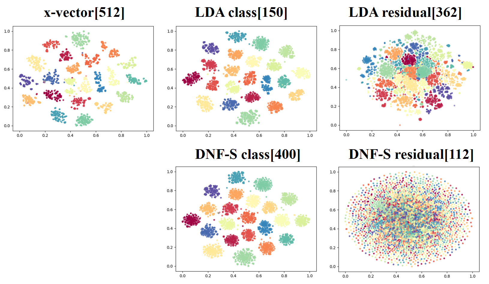
Fig. 4: Distributions of the latent codes in the class space and the residual space. Each color represents a speaker, and each point represents a speaker vector. The pictures are plotted by using t-SNE [25].

6 Conclusions

This paper interpret the discriminative normalization flow (DNF) as a deep generative LDA, and presents a subspace DNF that can perform nonlinear dimension reduction. Our analysis shows that our model represents a natural nonlinear extension for LDA while keeping almost all its valuable features, e.g., data explanation and data generation. Experiments on a simulation task and a practical speaker recognition task demonstrated that DNF and its subspace version are highly effective in modeling complex data and retrieving low-dimensional representation for them.

References

- [1] Ronald A Fisher, “The use of multiple measurements in taxonomic problems,” Annals of eugenics, vol. 7, no. 2, pp. 179–188, 1936.
- [2] NA Campbell, “Canonical variate analysis—a general model formulation,” Australian journal of statistics, vol. 26, no. 1, pp. 86–96, 1984.
- [3] Alok Sharma and Kuldip K Paliwal, “Linear discriminant analysis for the small sample size problem: an overview,” International Journal of Machine Learning and Cybernetics, vol. 6, no. 3, pp. 443–454, 2015.
- [4] Peter N. Belhumeur, João P Hespanha, and David J. Kriegman, “Eigenfaces vs. fisherfaces: Recognition using class specific linear projection,” IEEE Transactions on pattern analysis and machine intelligence, vol. 19, no. 7, pp. 711–720, 1997.
- [5] Bernhard Scholkopft and Klaus-Robert Mullert, “Fisher discriminant analysis with kernels,” Neural networks for signal processing IX, vol. 1, no. 1, pp. 1, 1999.
- [6] Robert Engle, ARCH: selected readings, Oxford University Press, 1995.
- [7] Nagendra Kumar and Andreas G Andreou, “Heteroscedastic discriminant analysis and reduced rank hmms for improved speech recognition,” Speech communication, vol. 26, no. 4, pp. 283–297, 1998.
- [8] Alaa Tharwat, “Linear vs. quadratic discriminant analysis classifier: a tutorial,” International Journal of Applied Pattern Recognition, vol. 3, no. 2, pp. 145–180, 2016.
- [9] Trevor Hastie and Robert Tibshirani, “Discriminant analysis by Gaussian mixtures,” Journal of the Royal Statistical Society: Series B (Methodological), vol. 58, no. 1, pp. 155–176, 1996.
- [10] Sebastian Mika, Gunnar Ratsch, Jason Weston, Bernhard Scholkopf, and Klaus-Robert Mullers, “Fisher discriminant analysis with kernels,” in Neural networks for signal processing IX: Proceedings of the 1999 IEEE signal processing society workshop (cat. no. 98th8468). Ieee, 1999, pp. 41–48.
- [11] Ian Goodfellow, Yoshua Bengio, Aaron Courville, and Yoshua Bengio, Deep learning, vol. 1, MIT press Cambridge, 2016.
- [12] Matthias Dorfer, Rainer Kelz, and Gerhard Widmer, “Deep linear discriminant analysis,” arXiv preprint arXiv:1511.04707, 2015.
- [13] Yunqi Cai, Lantian Li, Dong Wang, and Andrew Abel, “Deep normalization for speaker vectors,” arXiv preprint arXiv:2004.04095, 2020.
- [14] Walter Rudin, Real and complex analysis, Tata McGraw-hill education, 2006.
- [15] George Papamakarios, Eric Nalisnick, Danilo Jimenez Rezende, Shakir Mohamed, and Balaji Lakshminarayanan, “Normalizing flows for probabilistic modeling and inference,” arXiv preprint arXiv:1912.02762, 2019.
- [16] Laurent Dinh, Jascha Sohl-Dickstein, and Samy Bengio, “Density estimation using real nvp,” arXiv preprint arXiv:1605.08803, 2016.
- [17] George Papamakarios, Theo Pavlakou, and Iain Murray, “Masked autoregressive flow for density estimation,” in Advances in Neural Information Processing Systems, 2017, pp. 2338–2347.
- [18] Andre Stuhlsatz, Jens Lippel, and Thomas Zielke, “Feature extraction with deep neural networks by a generalized discriminant analysis,” IEEE transactions on neural networks and learning systems, vol. 23, no. 4, pp. 596–608, 2012.
- [19] Sergey Ioffe, “Probabilistic linear discriminant analysis,” in European Conference on Computer Vision (ECCV). Springer, 2006, pp. 531–542.
- [20] Arsha Nagrani, Joon Son Chung, and Andrew Zisserman, “Voxceleb: a large-scale speaker identification dataset,” arXiv preprint arXiv:1706.08612, 2017.
- [21] Joon Son Chung, Arsha Nagrani, and Andrew Zisserman, “Voxceleb2: Deep speaker recognition,” in Proceedings of the Annual Conference of International Speech Communication Association (INTERSPEECH), 2018, pp. 1086–1090.
- [22] Mitchell McLaren, Luciana Ferrer, Diego Castan, and Aaron Lawson, “The speakers in the wild (SITW) speaker recognition database.,” in Proceedings of the Annual Conference of International Speech Communication Association (INTERSPEECH), 2016, pp. 818–822.
- [23] Yue Fan, Jiawen Kang, Lantian Li, Kaicheng Li, Haolin Chen, Sitong Cheng, Pengyuan Zhang, Ziya Zhou, Yunqi Cai, and Dong Wang, “CN-CELEB: a challenging Chinese speaker recognition dataset,” arXiv preprint arXiv:1911.01799, 2019.
- [24] Daniel Povey, Arnab Ghoshal, Gilles Boulianne, Lukas Burget, Ondrej Glembek, Nagendra Goel, Mirko Hannemann, Petr Motlicek, Yanmin Qian, Petr Schwarz, et al., “The Kaldi speech recognition toolkit,” in IEEE 2011 workshop on automatic speech recognition and understanding. IEEE Signal Processing Society, 2011.
- [25] Laurens van der Maaten and Geoffrey Hinton, “Visualizing data using t-sne,” Journal of machine learning research, vol. 9, no. Nov, pp. 2579–2605, 2008.