Analysis of a greedy reconstruction algorithm

Abstract

A novel and detailed convergence analysis is presented for a greedy algorithm that was introduced in [13] for operator reconstruction problems in the field of quantum mechanics. This algorithm is based on an offline/online decomposition of the reconstruction process and on an ansatz for the unknown operator obtained by an a priori chosen set of linearly independent matrices. The presented convergence analysis focuses on linear-quadratic (optimization) problems governed by linear differential systems and reveals the strong dependence of the performance of the greedy algorithm on the observability properties of the system and on the ansatz of the basis elements. Moreover, the analysis allows us to use a precise (and in some sense optimal) choice of basis elements for the linear case and led to the introduction of a new and more robust optimized greedy reconstruction algorithm. This optimized approach also applies to nonlinear Hamiltonian reconstruction problems, and its efficiency is demonstrated by numerical experiments.

65K10, 81Q93, 34A55, 49N10, 49N45

1 Introduction

The identification of Hamiltonian operators plays a fundamental role in the fields of quantum physics and quantum chemistry; see, e.g., [6, 8, 9, 10, 20, 21, 22, 23, 24, 18] and references therein. Even though the overall literature about Hamiltonian identification problems is quite extensive, the mathematical contribution to this area is rather limited. Important mathematical theoretical contributions can be found in [3, 2] and in [12, 7], where uniqueness results for quantum inverse problems are proved by exploiting controllability arguments. Other techniques, based on the so-called Carleman’s estimate, are used in [2] to deduce uniqueness results for inverse problems governed by Schrödinger-type equations in presence of discontinuous coefficients. Excluding these few theoretical results, the literature rather focuses on numerical algorithms.

The term Hamiltonian identification often refers to two distinct problems. On the one hand, it sometimes indicates the inverse problem associated with the identification of a Hamiltonian operator obtained by a numerical fitting of simulated and given experimental data. On the other hand, it occasionally refers to both the problem of designing experimental parameters (allowing an optimized production of experimental data) and the subsequent inverse identification problem. In general, the design of experimental parameters includes the computation of control functions allowing an efficient numerical solving of the inverse problem.

In the latter problem, the algorithms proposed in the literature often combine the computation of control functions with the production of new synthetic (simulated) data or experimental data. Mathematically, this framework has given rise to two different approaches. The first one [12] consists in a procedure that alternately updates a (shrinking) set of admissible Hamiltonian operators and the trial control field used to generate new data. The second approach [13] is based on a full offline/online decomposition and is inspired by the greedy strategy emerged in the field of approximation theory in the 2000s; see, e.g., [1] and references therein. Even though some mathematical investigations of the first approach can be found in the literature (see [12, 7]), much less is known about the second strategy, for which only preliminary numerical results were presented in [13].

The goal of the present work is to provide a first detailed convergence analysis of the Hamiltonian reconstruction strategy defined in [13]. As a by-product, this analysis allows us to introduce a new more efficient and robust numerical reconstruction algorithm.

The numerical strategy presented in [13] is based on the ansatz that the unknown operator can be written as a linear combination of a priori given linearly independent matrices. The set of these matrices is denoted by $\mathcal{B}_{\mu}$. The reconstruction process is then decomposed in offline phase and online phase. In the offline phase, a family of control functions is built iteratively in a greedy manner in order to maximize the distinguishability of the system. This phase exploits only the quantum model, without any use of laboratory information. The algorithm proposed in [13] for the offline phase, that we call in this paper greedy reconstruction (GR) algorithm, consists of a sweep over the elements of $\mathcal{B}_{\mu}$. At every iteration of the GR algorithm, one new element of $\mathcal{B}_{\mu}$ is considered and a new control function is computed with the goal of splitting the states generated by the new element and the ones already considered in the previous iterations. The computed control functions are experimentally implemented in the online phase to produce laboratory data. These are in turn used to define and solve an identification inverse problem, aiming at fitting the numerical simulations with the corresponding experimental data.

In [13] the heuristic motivation for the offline phase is that this attempts to produce a set of control functions that make the online identification problem uniquely solvable (and easier to be solved) in a neighborhood of the true solution. Starting from this idea we develop a detailed convergence analysis for linear problems (linear-quadratic in the least-squares sense). Our analysis relates very clearly the iterations of the offline phase, and the corresponding computed control functions, to the solvability of the online identification problem. Moreover, the obtained theoretical results will reveal the strong dependence of the performance of the greedy reconstruction algorithm on the observability properties of the system and on the ansatz of the basis elements used to reconstruct the unknown operator. These observations allow us to improve the GR algorithm and introduce a new optimized greedy reconstruction (OGR) algorithm which shows a very robust behavior not only for the linear-quadratic reconstruction problems, but also for nonlinear Hamiltonian reconstruction problems.

The paper is organized as follows. In Section 2, the notation used throughout this paper is fixed. Section 3 describes the Hamiltonian reconstruction problem and the original GR algorithm introduced in [13]. The GR algorithm is then adapted to linear-quadratic problems in Section 4 and the corresponding convergence analysis is presented in Section 5. In Section 6, we introduce some improvements of the GR algorithm that lead to an optimized greedy reconstruction algorithm. The OGR algorithm is presented first for linear-quadratic problems and then extend to nonlinear Hamiltonian reconstruction problems. Within Section 6, results of numerical experiments are shown to demonstrate the efficiency and the improved robustness of the new proposed algorithm. Finally, we present our conclusions in Section 7.

2 Notation

Consider a positive natural number $N$. We denote by $\big{\langle}{\bf v},{\bf w}\big{\rangle}:=\overline{{\bf v}}^{\top}{\bf w}$, for any ${\bf v},{\bf w}\in\mathbb{C}^{N}$ the usual complex scalar product on $\mathbb{C}^{N}$, and by $\left\lVert\,\cdot\,\right\rVert_{2}$ the corresponding norm. Further, $|\,z\,|$ is the modulus of a complex number $z$ and $i$ is the imaginary unit. The space of symmetric matrices in $\mathbb{R}^{N\times N}$ is denoted by ${\rm Sym}(N)$. For any $A\in\mathbb{R}^{N\times N}$, $[A]_{j,k}$ denotes the $j,k$ (with $j,k\leq N$) entry of $A$ and the notation $A_{[1:k,1:j]}$ indicates the upper left submatrix of $A$ of size $k\times j$, namely $[A_{[1:k,1:j]}]_{\ell,m}:=[A]_{\ell,m}$ for $\ell=1,\dots,k$ and $m=1,\dots,j$. Similarly, $A_{[1:k,j]}$ denotes the column vector in $\mathbb{R}^{k}$ corresponding to the first $k$ elements of the column $j$ of $A$, namely $[A_{[1:k,j]}]_{\ell}:=[A]_{\ell,j}$ for $\ell=1,\dots,k$. Finally, the usual inner product of $L^{2}(0,T;\mathbb{C}^{N})$ is denoted by $\big{\langle}\cdot,\cdot\big{\rangle}_{L^{2}}$, and $L^{2}:=L^{2}(0,T;\mathbb{R})$.

3 Hamiltonian reconstruction and a greedy reconstruction algorithm

Consider the finite-dimensional Schrödinger equation

(1) $$\begin{split}i\dot{\boldsymbol{\psi}}(t)&=[H+\epsilon(t)\mu^{\star}]\boldsymbol{\psi}(t),\quad t\in(0,T],\\ \boldsymbol{\psi}(0)&=\boldsymbol{\psi}_{0},\end{split}$$

governing the time evolution of the state of a quantum system $\boldsymbol{\psi}\in\mathbb{C}^{N}$, $N\in\mathbb{N}^{+}$. The internal Hamiltonian $H$ is assumed to be known and the goal is to identify the unknown dipole moment operator $\mu^{\star}$ that couples the quantum system to a time-dependent external laser field $\epsilon\in L^{2}$, which acts as a control function on the system. Both internal Hamiltonian $H$ and dipole operator $\mu^{\star}$ belong to ${\rm Sym}(N)$, and $\boldsymbol{\psi}(t)$ lies in $\mathbb{C}^{N}$. The initial condition is $\boldsymbol{\psi}_{0}\in\mathbb{C}^{N}$ which satisfies $\left\lVert\boldsymbol{\psi}_{0}\right\rVert_{2}=1$.

The true dipole operator $\mu^{\star}$ is unknown and assumed to lie in a space spanned by $K$ linearly independent matrices $\mu_{1},\ldots,\mu_{K}$, forming the set $\mathcal{B}_{\mu}=(\mu_{j})_{j=1}^{K}\subset{\rm Sym}(N)$, where $K\in\mathbb{N}$ satisfies $1\leq K\leq{\rm dim\,Sym}(N)=\frac{N(N+1)}{2}$. Hence, we write $\mu^{\star}=\mu(\boldsymbol{\alpha}^{\star})$, with $\mu(\boldsymbol{\alpha}):=\sum_{j=1}^{K}\boldsymbol{\alpha}_{j}\mu_{j}$ for any $\boldsymbol{\alpha}\in\mathbb{R}^{K}$.

To identify the true operator $\mu^{\star}$ one uses a set of control fields $(\epsilon^{m})_{m=1}^{K}\subset L^{2}$ to perform $K$ laboratory experiments and obtain the experimental data

$$\varphi(\mu^{\star},\epsilon^{m}):=\big{\langle}\boldsymbol{\psi}_{1},\boldsymbol{\psi}_{T}(\mu^{\star},\epsilon^{m})\big{\rangle},\text{ for $m=1,\dots,K$}.$$

Here, $\boldsymbol{\psi}_{T}(\mu^{\star},\epsilon)$ denotes the solution to (1) at time $T>0$, corresponding to the dipole operator $\mu^{\star}$ and a laser field $\epsilon$. The value $\boldsymbol{\psi}_{1}\in\mathbb{C}^{N}$ is a fixed state with $\left\lVert\boldsymbol{\psi}_{1}\right\rVert_{2}=1$ and acts on a state of the quantum system as an observer operator. The measurements are assumed not to be affected by any type of noise.

Using the set of control fields $(\epsilon^{m})_{m=1}^{K}$ and the corresponding experimental data $(\varphi(\mu^{\star},\epsilon^{m}))_{m=1}^{K}\subset\mathbb{C}$, one solves the nonlinear least-squares problem

(2) $$\min_{\boldsymbol{\alpha}\in\mathbb{R}^{K}}\sum_{m=1}^{K}|\varphi(\mu^{\star},\epsilon^{m})-\varphi(\mu(\boldsymbol{\alpha}),\epsilon^{m})|^{2},$$

where $\varphi(\mu(\boldsymbol{\alpha}),\epsilon^{m}):=\big{\langle}\boldsymbol{\psi}_{1},\boldsymbol{\psi}_{T}(\mu(\boldsymbol{\alpha}),\epsilon^{m})\big{\rangle}$, with $\boldsymbol{\psi}_{T}(\mu(\boldsymbol{\alpha}),\epsilon^{m})$ the solution to (1) evaluated at time $T$ corresponding to the dipole operator $\mu(\boldsymbol{\alpha})$ and the laser field $\epsilon^{m}$. Clearly $\mu(\boldsymbol{\alpha}^{\star})$ is a global solution to (2).

If the control functions $(\epsilon^{m})_{m=1}^{K}$ and the data $(\varphi(\mu^{\star},\epsilon^{m}))_{m=1}^{K}$ are given, problem (2) is a standard parameter-identification inverse problem written in a minimization form. The choice of the laser fields $(\epsilon^{m})_{m=1}^{K}$ can affect significantly the properties of (2) and the corresponding solutions. To design an optimized set of control functions, in particular with the goal of improving local convexity properties of (2), Maday and Salomon introduced in [13] a numerical strategy which separates the reconstruction process of $\mu^{\star}$ in offline and online phases. In the offline phase, a greedy reconstruction (GR) algorithm computes a set of optimized laser fields $(\epsilon^{m})_{m=1}^{K}$ by exploiting only the quantum model (2) and without using any laboratory data. In the online phase, the computed control fields $(\epsilon^{m})_{m=1}^{K}$ are used experimentally to produce the laboratory data $\varphi(\mu^{\star},\epsilon^{m}):=\big{\langle}\boldsymbol{\psi}_{1},\boldsymbol{\psi}_{T}(\mu^{\star},\epsilon^{m})\big{\rangle}$ and to solve the nonlinear problem (2).

While the online phase consists (mathematically) in solving a classical parameter-identification inverse problem, the offline phase requires the GR algorithm introduced in [13]. The ideal goal of this offline/online framework is to find a good approximation of the unknown operator for which the difference at time $T$ between observed experimental data and numerically computed data is the smallest for any control. In other words, one aims at finding a matrix $\mu$ that solves

(3) $$\min_{\mu\in\text{span}\,\mathcal{B}_{\mu}}\;\;\max_{\epsilon\in L^{2}}|\varphi(\mu^{\star},\epsilon)-\varphi(\mu,\epsilon)|^{2},$$

or equivalently an $\boldsymbol{\alpha}$ that solves

(4) $$\min_{\boldsymbol{\alpha}\in\mathbb{R}^{K}}\;\;\max_{\epsilon\in L^{2}}|\varphi(\mu(\boldsymbol{\alpha}^{\star}),\epsilon)-\varphi(\mu(\boldsymbol{\alpha}),\epsilon)|^{2}.$$

Therefore, the goal of the GR algorithm is to generate a set of $K$ control functions such that a computed solution to (2) is also a solution to (3)-(4). To do so, the heuristic argument used in [13] is that the GR algorithm must attempt to distinguish numerical data for any two $\mu(\widetilde{\boldsymbol{\alpha}}),\mu(\widehat{\boldsymbol{\alpha}})\in{\rm span}\,\mathcal{B}_{\mu}$, $\mu(\widetilde{\boldsymbol{\alpha}})\neq\mu(\widehat{\boldsymbol{\alpha}})$, without performing any laboratory experiment. Following this idea, Maday and Salomon defined the GR algorithm as an iterative procedure that performs a sweep over the linearly independent matrices $(\mu_{k})_{k=1}^{K}$ and computes a new control field $\epsilon^{k+1}$ at each iteration. Suppose that the control fields $\epsilon^{1},\dots,\epsilon^{k}$ are already computed, the new control function $\epsilon^{k+1}$ is obtained by two sub-steps: one first solves the identification problem

(5) $$\min_{\boldsymbol{\alpha}_{1},\dots,\boldsymbol{\alpha}_{k}}\sum_{m=1}^{k}\Bigl{|}\varphi(\sum_{j=1}^{k}\boldsymbol{\alpha}_{j}\mu_{j},\epsilon^{m})-\varphi(\mu_{k+1},\epsilon^{m})\Bigr{|}^{2},$$

which gives the coefficients $\boldsymbol{\alpha}_{1}^{k},\dots,\boldsymbol{\alpha}_{k}^{k}$, and then computes the new field as

(6) $$\epsilon^{k+1}\in\hbox{argmax}_{\epsilon\in L^{2}}\Bigl{|}\varphi(\mu_{k+1},\epsilon)-\varphi\Bigl{(}\sum_{j=1}^{k}\boldsymbol{\alpha}_{j}^{k}\mu_{j},\epsilon\Bigr{)}\Bigr{|}^{2}.$$

The step of solving Problem (5) is called fitting step, since one attempts to compute a vector $\boldsymbol{\alpha}^{k}:=[\boldsymbol{\alpha}_{1}^{k},\dots,\boldsymbol{\alpha}_{k}^{k}]^{\top}$ that fits the quantities $\varphi(\sum_{j=1}^{k}\boldsymbol{\alpha}_{j}^{k}\mu_{j},\epsilon^{m})$ and $\varphi(\mu_{k+1},\epsilon^{m})$. In other words, the new basis element $\mu_{k+1}$ is considered and one identifies an element $\mu^{k}(\boldsymbol{\alpha}^{k}):=\sum_{j=1}^{k}\boldsymbol{\alpha}_{j}^{k}\mu_{j}$ such that none of the already computed control functions $\epsilon^{1},\dots,\epsilon^{k}$ is capable of distinguishing the observations $\varphi(\mu^{k}(\boldsymbol{\alpha}^{k}),\epsilon)$ and $\varphi(\mu_{k+1},\epsilon)$ (namely $\varphi(\mu^{k}(\boldsymbol{\alpha}^{k}),\epsilon^{m})\neq\varphi(\mu_{k+1},\epsilon^{m})$ for $m=1,\dots,k$). The step of solving problem (6) is called discriminatory step, because one computes a control function $\epsilon^{k+1}$ that is capable of distinguishing (discriminating) $\varphi(\mu^{k}(\boldsymbol{\alpha}^{k})\mu_{j},\epsilon^{k+1})$ from $\varphi(\mu_{k+1},\epsilon^{k+1})$.

The full GR algorithm is stated in Algorithm 1.

Algorithm 1 Greedy Reconstruction Algorithm

0:  A set of $K$ linearly independent matrices $\mathcal{B}_{\mu}=(\mu_{1},\ldots,\mu_{K})$.

1:  Solve the initialization problem

(7) $$\max\limits_{\boldsymbol{\epsilon}\in L^{2}}|\varphi(\mu_{1},\epsilon)-\varphi(0,0)|^{2}.$$

which gives the field $\epsilon^{1}$ and set $k=1$.

2:  while  $k\leq K-1$  do

3:     Fitting step: Find $(\boldsymbol{\alpha}^{k}_{j})_{j=1,\dots,k}$ that solve the problem

(8) $$\min\limits_{\boldsymbol{\alpha}\in\mathbb{R}^{k}}\sum_{m=1}^{k}|\varphi(\mu_{k+1},\epsilon^{m})-\varphi(\mu^{k}(\boldsymbol{\alpha}),\epsilon^{m})|^{2}.$$

4:     Discriminatory step: Find $\epsilon^{k+1}$ that solves the problem

(9) $$\max\limits_{\epsilon\in L^{2}}|\varphi(\mu_{k+1},\epsilon)-\varphi(\mu^{k}(\boldsymbol{\alpha}^{k}),\epsilon)|^{2}.$$

5:     Update $k\leftarrow k+1$.

6:  end while

Notice how the algorithm is obtained by a sequence of minimization and maximization problems, mimicking exactly the structure of the min-max problem (3)-(4).

Notice also that, since the goal of the GR algorithm is to compute control functions that allow one to distinguish between the states of the system corresponding to any possible dipole matrix, the algorithm implicitly attempts to compute control functions that make the online identification problem (2) locally strictly convex (hence uniquely solvable). This is an important observation that we will use to begin our convergence analysis.

Let us conclude this section with a final remark about the laboratory measurements. Throughout this paper, these are assumed to be not affected by any type of noise, even though noise is a significant factor that has to be dealt with; see [12, Remark 1] and references therein. However, the main goal of the present work is the numerical and convergence analysis of the computational framework and the GR algorithm introduced in [13], where noisy effects in taking measurements are also neglected.

4 Linear-quadratic reconstruction problems

Consider a state $\boldsymbol{y}$ whose time evolution is governed by the (real) ordinary differential equation

(10) $$\begin{split}\dot{\boldsymbol{y}}(t)&=A\boldsymbol{y}(t)+B^{\star}\boldsymbol{\epsilon}(t),\quad t\in(0,T],\\ \boldsymbol{y}(0)&=\boldsymbol{y}_{0},\end{split}$$

where $A\in\mathbb{R}^{N\times N}$ is a given matrix for $N\in\mathbb{N}^{+}$, the initial condition is $\boldsymbol{y}_{0}\in\mathbb{R}^{N}$, and $\boldsymbol{\epsilon}\in E_{ad}$ denotes a control function belonging to $E_{ad}$, a non-empty and weakly compact subset of $L^{2}(0,T;\mathbb{R}^{M})$ (e.g., a closed, convex and bounded subset of $L^{2}(0,T;\mathbb{R}^{M})$). The true control matrix $B^{\star}\in\mathbb{R}^{N\times M}$, for $M\in\mathbb{N}^{+}$, is unknown and assumed to lie in the space spanned by a set of linearly independent matrices $\mathcal{B}=\{B_{1},\ldots,B_{K}\}\subset\mathbb{R}^{N\times M}$, $1\leq K\leq NM$, and we write $B^{\star}=\sum_{j=1}^{K}\boldsymbol{\alpha}_{j}^{\star}B_{j}=:B(\boldsymbol{\alpha}^{\star})$.

As in the case of the Hamiltonian reconstruction problem, to identify the unknown matrix $B^{\star}$ one can consider a set of control functions $(\boldsymbol{\epsilon}^{m})_{m=1}^{K}\subset E_{ad}$ and use it experimentally to obtain the data $C\boldsymbol{y}_{T}(B^{\star},\boldsymbol{\epsilon}^{m})$, $m=1,\dots,K$. Here, $\boldsymbol{y}_{T}(B^{\star},\boldsymbol{\epsilon})$ denotes the solution of (10) at time $T$ and corresponding to a control function $\boldsymbol{\epsilon}$ and to the control matrix $B^{\star}$. Further, $C\in\mathbb{R}^{P\times N}$ is a given observer matrix.

As in Section 3, the reconstruction process is split into online and offline phases. In the offline phase, the GR algorithm computes the control functions $(\boldsymbol{\epsilon}^{m})_{m=1}^{K}$. These are then used in the online phase, in which the laboratory data

$$C\boldsymbol{y}_{T}(B^{\star},\boldsymbol{\epsilon}^{m}),\;m=1,\dots,K$$

are obtained and the identification problem

(11) $$\min_{\boldsymbol{\alpha}\in\mathbb{R}^{K}}\sum_{m=1}^{K}\left\lVert C\boldsymbol{y}_{T}(B^{\star},\boldsymbol{\epsilon}^{m})-C\boldsymbol{y}_{T}(B(\boldsymbol{\alpha}),\boldsymbol{\epsilon}^{m})\right\rVert_{2}^{2}$$

is solved.

As for the Hamiltonian reconstruction problem, the ideal goal of the offline/online framework is to find a good approximation of the unknown operator for which the norm difference at time $T$ between observed experimental data and numerically computed data is the smallest for any control function. In other words, we wish to find a matrix $B$ that solves

(12) $$\min_{B\in{\rm span}\,\mathcal{B}}\max_{\boldsymbol{\epsilon}\in E_{ad}}\left\lVert C\boldsymbol{y}_{T}(B^{\star},\boldsymbol{\epsilon})-C\boldsymbol{y}_{T}(B,\boldsymbol{\epsilon})\right\rVert_{2}^{2}$$

or equivalently

(13) $$\min_{\boldsymbol{\alpha}\in\mathbb{R}^{K}}\max_{\boldsymbol{\epsilon}\in E_{ad}}\left\lVert C\boldsymbol{y}_{T}(B^{\star},\boldsymbol{\epsilon})-C\boldsymbol{y}_{T}(B(\boldsymbol{\alpha}),\boldsymbol{\epsilon})\right\rVert_{2}^{2},$$

where $B(\boldsymbol{\alpha}):=\sum_{j=1}^{K}\boldsymbol{\alpha}_{j}B_{j}$. The GR algorithm generates a set of $K$ controls that attempt to distinguish numerical data for any two $B(\widehat{\boldsymbol{\alpha}})\neq B(\widetilde{\boldsymbol{\alpha}})$, without performing any laboratory experiment. The GR algorithm for linear-quadratic reconstruction problems is given in Algorithm 2.

Algorithm 2 Greedy Reconstruction Algorithm (linear-quadratic case)

0:  A set of $K$ linearly independent matrices $\mathcal{B}=(B_{1},\ldots,B_{K})$.

1:  Solve the initialization problem

(14) $$\max\limits_{\boldsymbol{\epsilon}\in E_{ad}}\left\lVert C\boldsymbol{y}_{T}(B_{1},\boldsymbol{\epsilon})-\boldsymbol{y}_{T}(0,0)\right\rVert_{2}^{2}.$$

which gives the field $\boldsymbol{\epsilon}^{1}$ and set $k=1$.

2:  while  $k\leq K-1$  do

3:     Fitting step: Find $(\boldsymbol{\alpha}^{k}_{j})_{j=1,\dots,k}$ that solve the problem

(15) $$\min\limits_{\boldsymbol{\alpha}\in\mathbb{R}^{k}}\sum_{m=1}^{k}\left\lVert C\boldsymbol{y}_{T}(B_{k+1},\boldsymbol{\epsilon}^{m})-C\boldsymbol{y}_{T}(B^{k}(\boldsymbol{\alpha}),\boldsymbol{\epsilon}^{m})\right\rVert_{2}^{2}.$$

4:     Discriminatory step: Find $\boldsymbol{\epsilon}^{k+1}$ that solves the problem

(16) $$\max\limits_{\boldsymbol{\epsilon}\in E_{ad}}\left\lVert C\boldsymbol{y}_{T}(B_{k+1},\boldsymbol{\epsilon})-C\boldsymbol{y}_{T}(B^{k}(\boldsymbol{\alpha}^{k}),\boldsymbol{\epsilon})\right\rVert_{2}^{2}.$$

5:     Update $k\leftarrow k+1$.

6:  end while

Since the convergence analysis performed in the next sections focuses on Algorithm 2, we wish to explain it in more details. The idea is to generate controls that separate the observations of system (10) at time $T$ for the different elements $B_{1},\ldots,B_{K}$, making possible the identification of their respective coefficients $\boldsymbol{\alpha}_{1}^{\star},\ldots,\boldsymbol{\alpha}_{K}^{\star}$ when solving (11). The initialization is performed by solving the optimal control problem (14), which aims at maximizing the distance (at time $T$) between the observed state of the uncontrolled system (namely $\boldsymbol{y}_{T}(0,0)$ corresponding to $\boldsymbol{\epsilon}=0$) and the observed state of the system

$$\begin{split}\dot{\boldsymbol{y}}(t)&=A\boldsymbol{y}(t)+B_{1}\boldsymbol{\epsilon}(t),\\ \boldsymbol{y}(0)&=\boldsymbol{y}_{0}.\end{split}$$

The numerical solution of this maximization problem provides the first control function $\boldsymbol{\epsilon}^{1}$.

Assume now that the control functions $\boldsymbol{\epsilon}^{1},\dots,\boldsymbol{\epsilon}^{k}$ are computed. The new element $\boldsymbol{\epsilon}^{k+1}$ is obtained by performing a fitting step (namely solving problem (15)) and a discriminatory step (namely solving problem (16)). In the fitting step, one compares the two systems

$$\begin{cases}\dot{\boldsymbol{y}}(t)=A\boldsymbol{y}(t)+B_{k+1}\boldsymbol{\epsilon}^{m}(t),\\ \boldsymbol{y}(0)=\boldsymbol{y}_{0},\end{cases}\qquad\quad\begin{cases}\dot{\boldsymbol{y}}(t)=A\boldsymbol{y}(t)+\biggl{(}\sum_{j=1}^{k}\boldsymbol{\alpha}_{j}B_{j}\biggr{)}\boldsymbol{\epsilon}^{m}(t),\\ \boldsymbol{y}(0)=\boldsymbol{y}_{0},\end{cases}$$

for $m\in\{1,\ldots,k\}$, and looks for an $\boldsymbol{\alpha}\in\mathbb{R}^{k}$ for which their observed solutions at time $T$ are as similar as possible (ideally the same, hence indistinguishable). We denote by $\boldsymbol{\alpha}^{k}=[\boldsymbol{\alpha}_{1}^{k},\dots,\boldsymbol{\alpha}_{k}^{k}]^{\top}$ the vector computed by solving (15). This vector is used in the subsequent discriminatory step, which consists in solving the optimal control problem (16). Here, we compute a control function $\boldsymbol{\epsilon}^{k+1}$ that maximizes the distance (at time $T$) between the solutions of the two systems

$$\begin{cases}\dot{\boldsymbol{y}}(t)=A\boldsymbol{y}(t)+B_{k+1}\boldsymbol{\epsilon}(t),\\ \boldsymbol{y}(0)=\boldsymbol{y}_{0},\end{cases}\qquad\quad\begin{cases}\dot{\boldsymbol{y}}(t)=A\boldsymbol{y}(t)+\sum_{j=1}^{k}\boldsymbol{\alpha}^{k}_{j}B_{j}\boldsymbol{\epsilon}(t),\\ \boldsymbol{y}(0)=\boldsymbol{y}_{0},\end{cases}$$

where now $\boldsymbol{\alpha}^{k}_{j}$ are fixed coefficients and the optimization variable is the control function $\boldsymbol{\epsilon}$. Notice that this maximization problem is well posed, as we will discuss in Lemma 5.3 in Section 5.

We wish to remark again that, since the goal of the GR algorithm is to compute control functions that permit to distinguish between the states of the system corresponding to any possible control matrix, the algorithm implicitly attempts to compute control functions that make the online identification problem locally uniquely solvable.

With these preparations, we are ready to present our convergence analysis.

5 Convergence Analysis

The convergence analysis presented in this section begins by recalling that one of the goals of the GR algorithm is to compute a set control functions that makes the online identification problem (11) strictly convex in a neighborhood of the solution $\boldsymbol{\alpha}^{\star}$ (and hence locally uniquely solvable). It is then natural to begin with problem (11) and prove the following lemma, which gives us an equivalent matrix-vector formulation.

Lemma 5.1 (Online identification problem in matrix form).

Problem (11) is equivalent to

(17) $$\min_{\boldsymbol{\alpha}\in\mathbb{R}^{K}}\;\big{\langle}\boldsymbol{\alpha}^{\star}-\boldsymbol{\alpha},\widehat{W}(\boldsymbol{\alpha}^{\star}-\boldsymbol{\alpha})\big{\rangle},$$

where $\widehat{W}\in\mathbb{R}^{K\times K}$ is defined as

(18) $$\widehat{W}:=\sum_{m=1}^{K}W(\boldsymbol{\epsilon}^{m}),$$

with $W(\boldsymbol{\epsilon}^{m})\in\mathbb{R}^{K\times K}$ given by

(19) $$[W(\boldsymbol{\epsilon}^{m})]_{\ell,j}:=\big{\langle}\boldsymbol{\gamma}_{\ell}(\boldsymbol{\epsilon}^{m}),\boldsymbol{\gamma}_{j}(\boldsymbol{\epsilon}^{m})\big{\rangle},\text{ for $\ell,j=1,\dots,K$},$$

and

(20) $$\boldsymbol{\gamma}_{\ell}(\boldsymbol{\epsilon}^{m}):=\int_{0}^{T}Ce^{(T-s)A}B_{\ell}\boldsymbol{\epsilon}^{m}(s)ds,\text{ for $m,\ell=1,\dots,K$}.$$

Proof 5.2.

Let us define

(21) $$J(\boldsymbol{\alpha}):=\sum_{m=1}^{K}\left\lVert C\boldsymbol{y}_{T}(B^{\star},\boldsymbol{\epsilon}^{m})-C\boldsymbol{y}_{T}(B(\boldsymbol{\alpha}),\boldsymbol{\epsilon}^{m})\right\rVert_{2}^{2},$$

and notice that

$$\boldsymbol{y}_{T}(B^{\star},\boldsymbol{\epsilon}^{m})=e^{TA}\boldsymbol{y}_{0}+\int_{0}^{T}e^{(T-s)A}\Big{(}\sum_{j=1}^{K}\boldsymbol{\alpha}_{j}^{\star}B_{j}\Big{)}\boldsymbol{\epsilon}^{m}(s)ds,$$

$$\boldsymbol{y}_{T}(B(\boldsymbol{\alpha}),\boldsymbol{\epsilon}^{m})=e^{TA}\boldsymbol{y}_{0}+\int_{0}^{T}e^{(T-s)A}\Big{(}\sum_{j=1}^{K}\boldsymbol{\alpha}_{j}B_{j}\Big{)}\boldsymbol{\epsilon}^{m}(s)ds.$$

The function $J(\boldsymbol{\alpha})$ can be written as

$$J(\boldsymbol{\alpha}) =\sum_{m=1}^{K}\left\lVert\int_{0}^{T}Ce^{(T-s)A}\Big{(}\sum_{j=1}^{K}(\boldsymbol{\alpha}_{j}^{\star}-\boldsymbol{\alpha}_{j})B_{\ell}\Big{)}\boldsymbol{\epsilon}^{m}(s)ds\right\rVert_{2}^{2}$$

$$=\sum_{m=1}^{K}\sum_{\ell=1}^{K}\sum_{j=1}^{K}(\boldsymbol{\alpha}_{\ell}^{\star}-\boldsymbol{\alpha}_{\ell})(\boldsymbol{\alpha}_{j}^{\star}-\boldsymbol{\alpha}_{j})\big{\langle}\boldsymbol{\gamma}_{\ell}(\boldsymbol{\epsilon}^{m}),\boldsymbol{\gamma}_{j}(\boldsymbol{\epsilon}^{m})\big{\rangle},$$

where the vectors $\boldsymbol{\gamma}_{\ell}(\boldsymbol{\epsilon}^{m})$ are defined in (20). We can now write

$$J(\boldsymbol{\alpha}) =\sum_{\ell=1}^{K}\sum_{j=1}^{K}(\boldsymbol{\alpha}_{\ell}^{\star}-\boldsymbol{\alpha}_{\ell})(\boldsymbol{\alpha}_{j}^{\star}-\boldsymbol{\alpha}_{j})\sum_{m=1}^{K}\big{\langle}\boldsymbol{\gamma}_{\ell}(\boldsymbol{\epsilon}^{m}),\boldsymbol{\gamma}_{j}(\boldsymbol{\epsilon}^{m})\big{\rangle}$$

$$=\big{\langle}\boldsymbol{\alpha}^{\star}-\boldsymbol{\alpha},\sum_{m=1}^{K}W(\boldsymbol{\epsilon}^{m})(\boldsymbol{\alpha}^{\star}-\boldsymbol{\alpha})\big{\rangle}=\big{\langle}\boldsymbol{\alpha}^{\star}-\boldsymbol{\alpha},\widehat{W}(\boldsymbol{\alpha}^{\star}-\boldsymbol{\alpha})\big{\rangle},$$

and the result follows.

Notice that, the matrices $W(\boldsymbol{\epsilon}^{m})$ defined in (19) can be written as $W(\boldsymbol{\epsilon}^{m})=\Gamma(\boldsymbol{\epsilon}^{m})^{\top}\Gamma(\boldsymbol{\epsilon}^{m})$, where $\Gamma(\boldsymbol{\epsilon}^{m})=[\boldsymbol{\gamma}_{1}(\boldsymbol{\epsilon}^{m})\,\cdots\,\boldsymbol{\gamma}_{K}(\boldsymbol{\epsilon}^{m})]$. Hence, $W(\boldsymbol{\epsilon}^{m})$ are symmetric and positive semi-definite. This guarantees that $\widehat{W}$ is also symmetric and positive semi-definite. Therefore, problem (17) is uniquely solved by $\boldsymbol{\alpha}=\boldsymbol{\alpha}^{\star}$ if and only if $\widehat{W}$ is positive definite, meaning that the GR algorithm actually aims at computing a set of control functions $(\boldsymbol{\epsilon}^{m})_{m=1}^{K}$ that makes $\widehat{W}$ positive definite. We then need to study how the positivity of $\widehat{W}$ evolves during the iteration of the algorithm. To do so, the first step is to rewrite the three problems (14), (15) and (16) also in a matrix-vector form.

Lemma 5.3 (The GR Algorithm 2 in matrix form).

Consider Algorithm 2. It holds that:

• The initialization problem (14) is equivalent to

  (22) $$\max_{\boldsymbol{\epsilon}\in E_{ad}}\;[W(\boldsymbol{\epsilon})]_{1,1}.$$

• The fitting-step problem (15) is equivalent to

  (23) $$\min_{\boldsymbol{\alpha}\in\mathbb{R}^{k}}\;\big{\langle}\boldsymbol{\alpha},\widehat{W}^{k}_{[1:k,1:k]}\boldsymbol{\alpha}\big{\rangle}-2\big{\langle}\widehat{W}^{k}_{[1:k,k+1]},\boldsymbol{\alpha}\big{\rangle},$$

  where $\widehat{W}^{k}$ is the $k$-th partial sum of $\widehat{W}$, that is $\widehat{W}^{k}=\sum_{m=1}^{k}W(\boldsymbol{\epsilon}^{m})$, and (recalling Section 2) $\widehat{W}^{k}_{[1:k,1:k]}\in\mathbb{R}^{k\times k}$ denotes the $k\times k$ upper-left block of $\widehat{W}^{k}$ and $\widehat{W}^{k}_{[1:k,k+1]}\in\mathbb{R}^{k}$ is a column vector containing the first $k$ components of the $k+1$-th column of $\widehat{W}^{k}$.

• The discriminatory-step problem (16) is equivalent to

  (24) $$\max_{\boldsymbol{\epsilon}\in E_{ad}}\;\big{\langle}\boldsymbol{v},[W(\boldsymbol{\epsilon})]_{[1:k+1,1:k+1]}\boldsymbol{v}\big{\rangle},$$

  where $W(\boldsymbol{\epsilon})$ is defined in (19) and $\boldsymbol{v}:=[(\boldsymbol{\alpha}^{k})^{\top},\;-1]^{\top}$.

Moreover, problems (14)-(22), (15)-(23), and (16)-(24) are well posed.

Proof 5.4.

The equivalences between (14), (15), (16) and (22), (23), and (24), respectively, can be proved by similar calculations to the one used in the proof of Lemma 5.1. We omit them for brevity.

Problem (15)-(23) is a quadratic minimization problem with quadratic function bounded from below by zero. Hence the existence of a minimizer follows.

Problems (14)-(22) and (16)-(24) are two classical optimal control problems. Since the admissible set $E_{ad}$ is a weakly compact subset of $L^{2}(0,T;\mathbb{R}^{M})$, the existence of a maximizer follows by standard arguments based on maximizing sequences and weak compactness; see, e.g., [4] and references therein.

Using the matrix representation given in Lemma 5.3, we can now sketch the mathematical meaning of the iterations of the GR algorithm. Assume that at the $k$-th iteration the submatrix $\widehat{W}^{k}_{[1:k,1:k]}$ is positive definite, but $\widehat{W}^{k}_{[1:k+1,1:k+1]}$ has a non-trivial (one-dimensional) kernel. The GR algorithm first tries to identify (by solving problem (23)) the kernel of $\widehat{W}^{k}_{[1:k+1,1:k+1]}$, and then attempts to compute (by solving problem (24)) a new control function $\boldsymbol{\epsilon}^{k+1}$ such that the matrix $W_{[1:k+1,1:k+1]}(\boldsymbol{\epsilon}^{k+1})$ is positive on the kernel $\widehat{W}^{k}_{[1:k+1,1:k+1]}$. If these happen, then the new updated matrix $\widehat{W}^{k+1}=\widehat{W}^{k}+W(\boldsymbol{\epsilon}^{k+1})$ has a positive definite upper-left block $\widehat{W}^{k+1}_{[1:k+1,1:k+1]}$. Moreover, if these two steps hold for any $k$, then the convergence follows since after the $K-1$-th iteration the matrix $\widehat{W}=\widehat{W}^{K}$ results to be positive definite. Hence, two questions clearly arise:

1. Does the fitting step of the algorithm always compute the non-trivial kernel of $\widehat{W}^{k}_{[1:k+1,1:k+1]}$ (in case it is truly non trivial)?

2. Does the discriminatory step of the algorithm always compute a control function $\boldsymbol{\epsilon}^{k+1}$ that makes $\widehat{W}^{k+1}_{[1:k+1,1:k+1]}$ positive definite?

The first question can be answered with the help of the following technical lemma.

Lemma 5.5 (On the kernel of symmetric positive semi-definite matrices).

Consider a symmetric, positive semi-definite matrix $\widetilde{G}\in\mathbb{R}^{n\times n}$ of the form

$$\widetilde{G}=\begin{bmatrix}G&\boldsymbol{b}\\ \boldsymbol{b}^{\top}&c\end{bmatrix},$$

where $G\in\mathbb{R}^{(n-1)\times(n-1)}$ is symmetric and positive definite and $\boldsymbol{b}\in\mathbb{R}^{n-1}$ and $c\in\mathbb{R}$ are such that the kernel of $\widetilde{G}$ is non-trivial. Then

$${\rm ker}(\widetilde{G})={\rm span}\bigg{\{}\begin{bmatrix}G^{-1}\boldsymbol{b}\\ -1\end{bmatrix}\bigg{\}}.$$

Proof 5.6.

Since the kernel of $\widetilde{G}$ is non-trivial, there exists a non-zero vector $\boldsymbol{u}=\begin{bmatrix}\boldsymbol{v}\\ d\end{bmatrix}\in\mathbb{R}^{n}\setminus\{0\}$ (with $\boldsymbol{v}\in\mathbb{R}^{n-1}$ and $d\in\mathbb{R}$) such that $\widetilde{G}\boldsymbol{u}=0$. Moreover, since $G$ is positive definite, the kernel of $\widetilde{G}$ must be one-dimensional and equal to the span of $\{\boldsymbol{u}\}$. Using the structure of $\boldsymbol{u}$, we write $\widetilde{G}\boldsymbol{u}=0$ as

(25) $$\begin{cases}G\boldsymbol{v}+d\;\boldsymbol{b}=0,\\ \boldsymbol{b}^{\top}\boldsymbol{v}+dc=0,\end{cases}\quad\overset{G\text{ invertible}}{\Longleftrightarrow}\quad\begin{cases}\boldsymbol{v}=-dG^{-1}\boldsymbol{b},\\ -d\;\boldsymbol{b}^{\top}G^{-1}\boldsymbol{b}+dc=0.\end{cases}$$

Now, suppose that $d=0$. This implies that $\boldsymbol{v}=-dG^{-1}\boldsymbol{b}=0$, which in turn implies that $\boldsymbol{u}=0$. However, this is a contradiction to the fact that $\boldsymbol{u}\neq 0$. Hence $d\neq 0$. The result follows by the right equations in (25) (divided by $-d$).

Recalling the equivalent form (23) of the fitting-step problem (15), one clearly see that, if $\widehat{W}^{k}_{[1:k,1:k]}$ is positive definite, then the unique solution to (23) is given by $\boldsymbol{\alpha}^{k}~{}=~{}(\widehat{W}^{k}_{[1:k,1:k]})^{-1}\widehat{W}^{k}_{[1:k,k+1]}$. On the other hand, if we set

$$\widetilde{G}=\widehat{W}^{k}_{[1:k+1,1:k+1]},\;G=\widehat{W}^{k}_{[1:k,1:k]},\;\boldsymbol{b}=\widehat{W}^{k}_{[1:k,k+1]},\;c=\widehat{W}^{k}_{[k+1,k+1]},$$

then Lemma 5.5 guarantees that the vector $\boldsymbol{v}:=[(\boldsymbol{\alpha}^{k})^{\top},\;-1]^{\top}$ spans the kernel of $\widehat{W}^{k}_{[1:k+1,1:k+1]}$, if this is non-trivial. Therefore, we have

$$\textnormal{ker}(\widehat{W}^{k}_{[1:k+1,1:k+1]}) =\textnormal{span}\Big{\{}\begin{bmatrix}(\widehat{W}^{k}_{[1:k,1:k]})^{-1}\widehat{W}^{k}_{[1:k,k+1]}\\ -1\end{bmatrix}\Big{\}}=\textnormal{span}\Big{\{}\boldsymbol{v}:=\begin{bmatrix}\boldsymbol{\alpha}^{k}\\ -1\end{bmatrix}\Big{\}}.$$

This means that, if $\widehat{W}^{k}_{[1:k+1,1:k+1]}$ has a rank defect, then the GR algorithm finds it by the splitting step.

The answer to the second question posed above is more complicated. In order to formulate it properly, we need to recall the definition of observability of an input/output dynamical system of the form

(26) $$\begin{split}\dot{\boldsymbol{y}}(t)&=A\boldsymbol{y}(t)+B\boldsymbol{\epsilon}(t),\quad\boldsymbol{y}(0)=\boldsymbol{y}_{0},\\ \boldsymbol{z}(t)&=C\boldsymbol{y}(t),\end{split}$$

with $A\in\mathbb{R}^{N\times N}$, $B\in\mathbb{R}^{N\times M}$, $C\in\mathbb{R}^{P\times N}$; see, e.g., [17].

Definition 5.7 (Observable input-output linear systems).

The input-output linear system (26) is said to be observable if the initial state $\boldsymbol{y}(0)=\boldsymbol{y}_{0}$ can be uniquely determined from input/output measurements. Equivalently, (26) is observable if and only if the observability matrix

(27) $$\mathcal{O}_{N}(C,A):=\begin{bmatrix}C\\ CA\\ \vdots\\ CA^{N-1}\end{bmatrix}$$

has full column rank.

Notice that the matrix $B$ does not affect the observability of system (26).

We now assume that the system is observable, namely that $\textnormal{rank}\;\mathcal{O}_{N}(C,A)=N$, and we show that this is a sufficient condition for the GR algorithm to make the matrix $\widehat{W}$ positive definite. To do so, we first prove the following lemma regarding the discriminatory step. Notice that the proof of this result is inspired by classical Kalmann controllability theory; see, e.g., [5].

Lemma 5.8 (Discriminatory-step problem for fully observable systems).

Assume that the matrices $A\in\mathbb{R}^{N\times N}$ and $C\in\mathbb{R}^{P\times N}$ are such that $\textnormal{rank }\mathcal{O}_{N}(C,A)=N$. Let $\widehat{W}^{k}_{[1:k,1:k]}$ be positive definite, $\boldsymbol{\alpha}^{k}$ the solution to the fitting-step problem (15), and $\boldsymbol{v}=[(\boldsymbol{\alpha}^{k})^{\top},-1]^{\top}$. Then any solution $\boldsymbol{\epsilon}^{k+1}$ of the discriminatory-step problem (16) satisfies

$$\big{\langle}\boldsymbol{v},W_{[1:k+1,1:k+1]}(\boldsymbol{\epsilon}^{k+1})\boldsymbol{v}\big{\rangle}=\left\lVert\int_{0}^{T}Ce^{(T-s)A}\Big{(}B_{k+1}-\sum_{j=1}^{k}\boldsymbol{\alpha}^{k}_{j}B_{j}\Big{)}\boldsymbol{\epsilon}^{k+1}(s)ds\right\rVert_{2}^{2}>0,$$

for $k=0,1,\dots,K-1$.

Proof 5.9.

Let us define $\widetilde{B}:=B_{k+1}-\sum_{j=1}^{k}\boldsymbol{\alpha}^{k}_{j}B_{j}$. Since the matrices $B_{1},\ldots,B_{k+1}$ are assumed to be linearly independent, $\widetilde{B}$ is non-zero.

Now, we consider an arbitrary $\delta\in(0,T)$ and define a control function $\widetilde{\boldsymbol{\epsilon}}\in E_{ad}$ as

$$\widetilde{\boldsymbol{\epsilon}}(s):=\begin{cases}0,&0\leq s<\delta,\\ \boldsymbol{e}_{i},&\delta\leq s\leq T,\end{cases}$$

where $\boldsymbol{e}_{i}\in\mathbb{R}^{M}$ is the $i$-th canonical vector for some index $1\leq i\leq M$. Further, we denote by $\widetilde{\boldsymbol{b}}_{i}$ the $i$-th column of $\widetilde{B}$. Since $\widetilde{B}$ is non-zero, we can choose the index $i$ such that $\widetilde{\boldsymbol{b}}_{i}\neq 0$. Now, we compute

$$\int_{0}^{T}Ce^{(T-s)A}\widetilde{B}\widetilde{\boldsymbol{\epsilon}}(s)ds =\int_{\delta}^{T}Ce^{(T-s)A}\widetilde{\boldsymbol{b}}_{i}ds=\int_{\delta}^{T}C\Big{[}\sum_{j=0}^{\infty}\frac{(T-s)^{j}A^{j}}{j!}\Big{]}\widetilde{\boldsymbol{b}}_{i}ds$$

$$\overset{(\star)}{=}\Big{[}\sum_{j=0}^{\infty}\int_{\delta}^{T}\frac{(T-s)^{j}}{j!}ds\;CA^{j}\Big{]}\widetilde{\boldsymbol{b}}_{i}=\Big{[}\sum_{j=0}^{\infty}\frac{(T-\delta)^{j+1}}{(j+1)!}CA^{j}\Big{]}\widetilde{\boldsymbol{b}}_{i}$$

$$=\sum_{j=0}^{\infty}\beta_{j}(\delta)CA^{j}\widetilde{\boldsymbol{b}}_{i},$$

where $\beta_{j}(\delta):=\frac{(T-\delta)^{j+1}}{(j+1)!}$ and we used the dominated convergence theorem (see, e.g., [15, Theorem 1.34]) to interchange integral and infinite sum and obtain the equality $(\star)$. Since the observability matrix $\mathcal{O}_{N}(C,A)$ has full rank and $\widetilde{\boldsymbol{b}}_{i}\neq 0$, there exists an index $0\leq j\leq N-1$ such that $CA^{j}\widetilde{\boldsymbol{b}}_{i}\neq 0$. Hence, $f(\delta):=\sum_{j=0}^{\infty}\beta_{j}(\delta)CA^{j}\widetilde{\boldsymbol{b}}_{i}$ is an analytic function for $\delta\in(0,T)$ and such that $f\neq 0$. We also know that (non-constant) analytic functions have isolated roots; see, e.g., [15, Theorem 10.18]. Therefore we can find a $\delta\in(0,T)$ such that $\sum_{j=0}^{\infty}\beta_{j}(\delta)CA^{j}\widetilde{\boldsymbol{b}}_{i}\neq 0$, and obtain the existence of an $\widetilde{\boldsymbol{\epsilon}}\in E_{ad}$ such that

$$\int_{0}^{T}Ce^{(T-s)A}\widetilde{B}\widetilde{\boldsymbol{\epsilon}}(s)ds\neq 0.$$

This implies that

$$\begin{split}\big{\langle}\boldsymbol{v},W_{[1:k+1,1:k+1]}(\boldsymbol{\epsilon}^{k+1})\boldsymbol{v}\big{\rangle}&=\left\lVert\int_{0}^{T}Ce^{(T-s)A}\Big{(}B_{k+1}-\sum_{\ell=1}^{k}\boldsymbol{\alpha}^{k}_{\ell}B_{\ell}\Big{)}\boldsymbol{\epsilon}^{k+1}(s)ds\right\rVert_{2}^{2}\\ &\geq\left\lVert\int_{0}^{T}Ce^{(T-s)A}\Big{(}B_{k+1}-\sum_{\ell=1}^{k}\boldsymbol{\alpha}^{k}_{\ell}B_{\ell}\Big{)}\widetilde{\boldsymbol{\epsilon}}(s)ds\right\rVert_{2}^{2}\\ &=\left\lVert\int_{0}^{T}Ce^{(T-s)A}\widetilde{B}\widetilde{\boldsymbol{\epsilon}}(s)ds\right\rVert_{2}^{2}>0,\end{split}$$

where we have used that $\boldsymbol{\epsilon}^{k+1}$ is a maximizer for problem (16).

Now we can prove our first main convergence result.

Theorem 5.10 (Convergence of the GR algorithm for fully observable systems).

Assume that the matrices $A\in\mathbb{R}^{N\times N}$ and $C\in\mathbb{R}^{P\times N}$ are such that $\textnormal{rank }\mathcal{O}_{N}(C,A)=N$. Let $K\in\{1,\dots,MN\}$ be arbitrary and let $\{\boldsymbol{\epsilon}^{1},\ldots,\boldsymbol{\epsilon}^{K}\}\subset E_{ad}$ be a family of controls generated by the GR Algorithm 2. Then the matrix $\widehat{W}$ defined in (18) is positive definite and online identification problem (11) is uniquely solvable by $\boldsymbol{\alpha}=\boldsymbol{\alpha}^{\star}$.

Proof 5.11.

By Lemma 5.1 it is sufficient to show that the matrix $\widehat{W}$ corresponding to the controls $\boldsymbol{\epsilon}^{1},\ldots,\boldsymbol{\epsilon}^{K}$ generated by the algorithm is positive definite. The proof of this claim proceeds by induction.

Lemma 5.8 guarantees that there exists an $\boldsymbol{\epsilon}^{1}$ such that $[W(\boldsymbol{\epsilon}^{1})]_{1,1}>0$. Now, we assume that $\widehat{W}^{k}_{[1:k,1:k]}$ is positive definite, and we show that $\widehat{W}^{k+1}_{[1:k+1,1:k+1]}$ is positive definite as well.

If $\widehat{W}^{k}_{[1:k+1,1:k+1]}$ is positive definite, then

$$\widehat{W}^{k+1}_{[1:k+1,1:k+1]}=\widehat{W}^{k}_{[1:k+1,1:k+1]}+W(\boldsymbol{\epsilon}^{k})_{[1:k+1,1:k+1]}$$

is positive definite as well, since $W(\boldsymbol{\epsilon}^{k})_{[1:k+1,1:k+1]}$ is positive semi-definite.

Assume now that the submatrix $\widehat{W}^{k}_{[1:k+1,1:k+1]}$ has a non-trivial kernel. Since $\widehat{W}^{k}_{[1:k,1:k]}$ is positive definite (induction hypothesis), problem (23) is uniquely solvable with solution $\boldsymbol{\alpha}^{k}$. Then, by Lemma 5.5 the (one-dimensional) kernel of $\widehat{W}^{k}_{[1:k+1,1:k+1]}$ is the span of the the vector $\boldsymbol{v}=[(\boldsymbol{\alpha}^{k})^{\top},\;-1]^{\top}$. Finally, using Lemma 5.8 we obtain that the solution $\boldsymbol{\epsilon}^{k+1}$ to the discriminatory-step problem satisfies

$$0<\big{\langle}\boldsymbol{v},[W(\boldsymbol{\epsilon}^{k+1})]_{[1:k+1,1:k+1]}\boldsymbol{v}\big{\rangle}.$$

Hence, the matrix $[W(\boldsymbol{\epsilon}^{k+1})]_{[1:k+1,1:k+1]}$ is positive definite on the span of $\boldsymbol{v}$. Therefore $\widehat{W}^{k+1}_{[1:k+1,1:k+1]}=\widehat{W}^{k}_{[1:k+1,1:k+1]}+[W(\boldsymbol{\epsilon}^{k+1})]_{[1:k+1,1:k+1]}$ is positive definite, and the claim follows.

Remark 5.12 (Uniqueness of solution of the min-max problem (13)).

Under the assumption that the system is fully observable, the min-max problem (13) is also uniquely solvable with $\boldsymbol{\alpha}=\boldsymbol{\alpha}^{\star}$. To see this, we first note that (13) can be written in terms of $W(\boldsymbol{\epsilon})$:

$$\left\lVert C\boldsymbol{y}_{T}(B^{\star},\boldsymbol{\epsilon})-C\boldsymbol{y}_{T}(B(\boldsymbol{\alpha}),\boldsymbol{\epsilon})\right\rVert^{2} =\left\lVert\int_{0}^{T}Ce^{(T-s)A}\Big{(}\sum_{j=1}^{K}(\boldsymbol{\alpha}_{j}-\boldsymbol{\alpha}^{\star}_{j})B_{j}\Big{)}\boldsymbol{\epsilon}(s)ds\right\rVert_{2}^{2}$$

$$=\big{\langle}(\boldsymbol{\alpha}-\boldsymbol{\alpha}^{\star}),W(\boldsymbol{\epsilon})(\boldsymbol{\alpha}-\boldsymbol{\alpha}^{\star})\big{\rangle}.$$

Now, similarly as in the proof of Lemma 5.8 and using the full observability of the system, one can show that for any $\widehat{\boldsymbol{\alpha}}\in\mathbb{R}^{NM}$ with $\widehat{\boldsymbol{\alpha}}\neq\boldsymbol{\alpha}^{\star}$ there exists a control $\boldsymbol{\epsilon}(\widehat{\boldsymbol{\alpha}})$ such that

$$\big{\langle}(\widehat{\boldsymbol{\alpha}}-\boldsymbol{\alpha}^{\star}),W(\boldsymbol{\epsilon}(\widehat{\boldsymbol{\alpha}}))(\widehat{\boldsymbol{\alpha}}-\boldsymbol{\alpha}^{\star})\big{\rangle}>0.$$

Therefore the unique solution to (13) is $\boldsymbol{\alpha}=\boldsymbol{\alpha}^{\star}$.

Notice that, Theorem 5.10 does not require any particular assumption on the matrices $B_{1},\dots,B_{K}$, which can be arbitrarily chosen with the only constraint to be linearly independent. Moreover, the number $K\in\{1,\dots,MN\}$ can be fixed arbitrarily and the GR algorithm will compute control functions that permit the exact reconstruction of the coefficients of the linear combination of the first $K$ components of $B^{\star}$ in a basis $\{B_{1},\dots,B_{MN}\}$. To be more precise, if the unknown $B^{\star}$ belongs to the span of $K$ the linearly independent matrices $B_{1},\dots,B_{K}$ used by the algorithm, then, using the control functions generated by the GR algorithm, the unknown $B^{\star}$ can be fully reconstructed. If $B^{\star}$ lies in the span of $\widetilde{K}\in\{K+1,K+2,\dots,MN\}$ linearly independent matrices $B_{1},\dots,B_{\widetilde{K}}$, but only the first $K$ of these are used by the algorithm (and in the online identification problem), then one reconstructs exactly the $K$ coefficients corresponding to the first elements $B_{1},\dots,B_{K}$. Furthermore, the ordering of the $K$ considered matrices does not affect the convergence result of Theorem 5.10.

These observations are no longer true if the system is non-fully observable, that is ${\rm rank}\,\mathcal{O}_{N}(C,A)=\mathcal{R}<N$. In this case, the choice of the linearly independent matrices $B_{1},\dots,B_{K}$ and their ordering become crucial for the algorithm. In particular, we are going to show that the method can recover at most $K=\mathcal{R}M$ components of the unknown vector $\boldsymbol{\alpha}^{\star}$, if appropriate matrices $B_{1},\dots,B_{K}$ are chosen. Moreover, we will see that an inappropriate choice of matrices $B_{1},\dots,B_{K}$ can lead to completely wrong results with an arbitrary error.

For our analysis, we begin by choosing a set of $K=NM$ matrices by exploiting the kernel of the observability matrix. In particular, recalling that ${\rm rank}\,\mathcal{O}_{N}(C,A)=\mathcal{R}<N$, the rank-nullity theorem allows us to consider a basis $\{\boldsymbol{v}_{j}\}_{j=1}^{N}\subset\mathbb{R}^{N}$ of $\mathbb{R}^{N}$, such that

(28) $$\boldsymbol{v}_{j}\notin\textnormal{ker}\;\mathcal{O}_{N}(C,A), \qquad\;j=1,\ldots,\mathcal{R},$$

(29) $$\boldsymbol{v}_{j}\in\textnormal{ker}\;\mathcal{O}_{N}(C,A), \qquad j=\mathcal{R}+1,\ldots,N,$$

where clearly $\textnormal{span}\{\boldsymbol{v}_{j}\}_{j=\mathcal{R}+1}^{N}=\textnormal{ker}\;\mathcal{O}_{N}(C,A)$. We now define a basis $\{B^{\mathcal{O}}_{k}\}_{k=1}^{NM}$ of $\mathbb{R}^{N\times M}$ as

(30) $$\begin{split}B^{\mathcal{O}}_{1}&=\boldsymbol{v}_{1}\boldsymbol{e}_{1}^{\top},\;B^{\mathcal{O}}_{2}=\boldsymbol{v}_{1}\boldsymbol{e}_{2}^{\top},\;\cdots,\;B^{\mathcal{O}}_{M}=\boldsymbol{v}_{1}\boldsymbol{e}_{M}^{\top},\\ B^{\mathcal{O}}_{M+1}&=\boldsymbol{v}_{2}\boldsymbol{e}_{1}^{\top},\;B^{\mathcal{O}}_{M+2}=\boldsymbol{v}_{2}\boldsymbol{e}_{2}^{\top},\;\cdots,\;B^{\mathcal{O}}_{2M}=\boldsymbol{v}_{2}\boldsymbol{e}_{M}^{\top},\\ &\vdots\qquad\qquad\qquad\vdots\qquad\qquad\qquad\vdots\\ B^{\mathcal{O}}_{(N-1)M+1}&=\boldsymbol{v}_{N}\boldsymbol{e}_{1}^{\top},\;B^{\mathcal{O}}_{(N-1)M+2}=\boldsymbol{v}_{N}\boldsymbol{e}_{2}^{\top},\;\cdots,\;B^{\mathcal{O}}_{NM}=\boldsymbol{v}_{N}\boldsymbol{e}_{M}^{\top},\end{split}$$

where $\boldsymbol{e}_{\ell}\in\mathbb{R}^{M}$, for $\ell=1,\dots,M$, are the canonical vectors in $\mathbb{R}^{M}$. Notice that, since the vectors $(\boldsymbol{v}_{j})_{j=1}^{N}$ are linearly independent, the set $\{B^{\mathcal{O}}_{k}\}_{k=1}^{NM}$ is clearly a basis of $\mathbb{R}^{N\times M}$.

From a computational point of view, the vectors $\boldsymbol{v}_{j}$ can be obtained by a singular value decomposition (SVD) of the observability matrix $\mathcal{O}_{N}(C,A)=U\Sigma V^{\top}$, where the columns of $V$ form a basis of $\mathbb{R}^{N}$ and the last $N-\mathcal{R}$ columns of $V$ span the kernel of $\mathcal{O}_{N}(C,A)$; see, e.g., [19, Theorem 5.2]. Therefore, one can set $\boldsymbol{v}_{j}=V_{[:,j]}$, $j=1,\ldots,N$.

Our first result for non-fully observable systems says that, if the basis $\{B^{\mathcal{O}}_{k}\}_{k=1}^{NM}$ is considered, then we can reduce the reconstruction of $B^{\star}=\sum_{j=1}^{MN}\boldsymbol{\alpha}_{j}^{\star}B^{\mathcal{O}}_{j}$ only to the first $\mathcal{R}M$ coefficients $\boldsymbol{\alpha}_{1},\dots,\boldsymbol{\alpha}_{\mathcal{R}M}$. This is proved in the next lemma, where we use the notation

$$B_{\mathcal{R}}(\boldsymbol{\alpha}^{\star}):=\sum_{j=1}^{\mathcal{R}M}\boldsymbol{\alpha}_{j}^{\star}B^{\mathcal{O}}_{j}.$$

Lemma 5.13 (Online identification problem for non-fully observable systems).

Consider the basis $\{B^{\mathcal{O}}_{k}\}_{k=1}^{NM}$ constructed as in (30) (with vectors $\boldsymbol{v}_{j}$, $j=1,\dots,N$, as in (28)-(29)). The online least-squares problem (11) (with $K=MN$) is equivalent to

(31) $$\min_{\boldsymbol{\alpha}\in\mathbb{R}^{\mathcal{R}M}}\;\sum_{m=1}^{NM}\left\lVert C\boldsymbol{y}_{T}(B^{\star},\boldsymbol{\epsilon}^{m})-C\boldsymbol{y}_{T}(B_{\mathcal{R}}(\boldsymbol{\alpha}),\boldsymbol{\epsilon}^{m})\right\rVert_{2}^{2}.$$

Proof 5.14.

Notice that, for any $\ell\in\{1,2,\dots,NM\}$ and $s\in[0,T]$, there exist $N$ functions $\widetilde{\beta}_{j}$ such that

$$Ce^{(T-s)A}B^{\mathcal{O}}_{\ell} =C\sum_{j=0}^{\infty}\frac{(T-s)^{j}}{j!}A^{j}B^{\mathcal{O}}_{\ell}\overset{(\star)}{=}C\Big{[}\sum_{j=0}^{N-1}\widetilde{\beta}_{j}(s)A^{j}\Big{]}B^{\mathcal{O}}_{\ell}$$

$$=\Big{[}\widetilde{\beta}_{0}(s)I_{N},\widetilde{\beta}_{1}(s)I_{N},\ldots,\widetilde{\beta}_{N-1}(s)I_{N}\Big{]}\mathcal{O}_{N}(C,A)B^{\mathcal{O}}_{\ell},$$

where we have used the Cayley-Hamilton theorem (see, e.g., [11, p.109]) to obtain the equality $(\star)$. If $\ell\in\{\mathcal{R}M+1,\ldots,NM\}$, then $B^{\mathcal{O}}_{\ell}=\boldsymbol{v}_{j}\boldsymbol{e}_{i}^{\top}$ with $j\geq\mathcal{R}+1$, hence $\boldsymbol{v}_{j}\in\textnormal{ker}\;\mathcal{O}_{N}(C,A)$ and therefore

$$\mathcal{O}_{N}(C,A)B^{\mathcal{O}}_{\ell}=\underbrace{\mathcal{O}_{N}(C,A)\boldsymbol{v}_{j}}_{=0}\boldsymbol{e}_{i}^{\top}=0.$$

This means that, for all $\ell\in\{\mathcal{R}M+1,\ldots,NM\}$ and $s\in[0,T]$, $Ce^{(T-s)A}B^{\mathcal{O}}_{\ell}=0$, and thus

$$\int_{0}^{T}Ce^{(T-s)A}B^{\mathcal{O}}_{\ell}\boldsymbol{\epsilon}(s)ds=0,$$

for any control function $\boldsymbol{\epsilon}\in E_{ad}$. Now, recalling the definition of $J(\boldsymbol{\alpha})$ from the proof of Lemma 5.1, we write the least-squares problem (11) as

$$J(\boldsymbol{\alpha}) =\sum_{m=1}^{NM}\left\lVert\sum_{j=1}^{NM}(\boldsymbol{\alpha}_{j}^{\star}-\boldsymbol{\alpha}_{j})\int_{0}^{T}Ce^{(T-s)A}B^{\mathcal{O}}_{j}\boldsymbol{\epsilon}^{m}(s)ds\right\rVert_{2}^{2}$$

$$=\sum_{m=1}^{NM}\left\lVert\sum_{j=1}^{\mathcal{R}M}(\boldsymbol{\alpha}_{j}^{\star}-\boldsymbol{\alpha}_{j})\int_{0}^{T}Ce^{(T-s)A}B^{\mathcal{O}}_{j}\boldsymbol{\epsilon}^{m}(s)ds\right\rVert_{2}^{2},$$

which is our claim.

Lemma 5.13 implies that the coefficients $\boldsymbol{\alpha}_{\mathcal{R}M+1},\dots,\boldsymbol{\alpha}_{MN}$ do not affect the cost function to be minimized. Therefore, any vector $\boldsymbol{\alpha}\in\mathbb{R}^{MN}$ of the form

$$\boldsymbol{\alpha}=[\boldsymbol{\alpha}_{1}^{\star},\cdots,\boldsymbol{\alpha}_{\mathcal{R}M}^{\star},\gamma_{\mathcal{R}M+1},\cdots,\gamma_{MN}]^{\top}$$

is a global solution to (11), for any $\gamma_{j}\in\mathbb{R}$, $j=\mathcal{R}M+1,\dots,MN$. This means that, one uses really only the first $\mathcal{R}M$ elements of the basis. In fact, as we are going to show in Lemma 5.15 and Theorem 5.17, only their corresponding coefficients can be reconstructed, while no information can be obtained for the remaining ones. It is therefore natural, for ${\rm rank}\,\mathcal{O}_{N}(C,A)=\mathcal{R}<N$, to use the GR algorithm with only the first $\mathcal{R}M$ basis elements $B^{\mathcal{O}}_{1},\dots,B^{\mathcal{O}}_{\mathcal{R}M}$. In this case, the proof of convergence for the GR algorithm is analogous to what we have done to obtain Theorem 5.10. We first prove a version of Lemma 5.8 adapted to non-fully observable systems.

Lemma 5.15 (Discriminatory-step problem for non-fully observable systems).

Assume that ${\rm rank}\,\mathcal{O}_{N}(C,A)=\mathcal{R}<N$ and that the GR algorithm is run until the $k$-th iteration, with $k<\mathcal{R}M$, using the linearly independent matrices $B^{\mathcal{O}}_{1},\dots,B^{\mathcal{O}}_{\mathcal{R}M}$ defined in (30). Let $\widehat{W}^{k}_{[1:k,1:k]}$ be positive definite, and let $\boldsymbol{\alpha}^{k}$ be the solution to the fitting-step problem (15). Then any solution $\boldsymbol{\epsilon}^{k+1}$ of the discriminatory-step problem (16) satisfies for $k=1,\ldots\mathcal{R}M-1$

$$\big{\langle}\boldsymbol{v},W_{[1:k+1,1:k+1]}(\boldsymbol{\epsilon}^{k+1})\boldsymbol{v}\big{\rangle}=\left\lVert\int_{0}^{T}Ce^{(T-s)A}\Big{(}B^{\mathcal{O}}_{k+1}-\sum_{j=1}^{k}\boldsymbol{\alpha}^{k}_{j}B^{\mathcal{O}}_{j}\Big{)}\boldsymbol{\epsilon}^{k+1}(s)ds\right\rVert_{2}^{2}>0,$$

where $\boldsymbol{v}:=[(\boldsymbol{\alpha}^{k})^{\top},\;-1]^{\top}$, for $k=0,1,\dots,K-1$.

Proof 5.16.

Notice that, since the matrices $B^{\mathcal{O}}_{1},\dots,B^{\mathcal{O}}_{\mathcal{R}M}$ are linearly independent and defined as in (30), we have that $\mathcal{O}_{N}(C,A)\Big{(}B^{\mathcal{O}}_{k+1}-\sum_{j=1}^{k}\boldsymbol{\alpha}^{k}_{j}B^{\mathcal{O}}_{j}\Big{)}\neq 0$.

With this observation, the result can be proved exactly as Lemma 5.8.

Using Lemma 5.15, we can prove convergence for the GR Algorithm 2 in case the matrices $B_{1},\dots,B_{\mathcal{R}M}$ defined in (30) are used.

Theorem 5.17 (Convergence of the GR alg. for non-fully observable systems).

Let $(\boldsymbol{\epsilon}^{m})_{m=1}^{\mathcal{R}M}\subset E_{ad}$ be a family of controls generated by the GR Algorithm 2 with $K\leq\mathcal{R}M$ and using the matrices $B^{\mathcal{O}}_{1},\dots,B^{\mathcal{O}}_{\mathcal{R}M}$ defined in (30). Then the least-squares problem

(32) $$\min_{\boldsymbol{\alpha}\in\mathbb{R}^{\mathcal{R}M}}\sum_{m=1}^{\mathcal{R}M}\left\lVert C\boldsymbol{y}_{T}(B^{\star},\boldsymbol{\epsilon}^{m})-C\boldsymbol{y}_{T}(B_{\mathcal{R}}(\boldsymbol{\alpha}),\boldsymbol{\epsilon}^{m})\right\rVert_{2}^{2}$$

is uniquely solvable with $\boldsymbol{\alpha}_{j}=\boldsymbol{\alpha}_{j}^{\star}$ for $j=1,\ldots,\mathcal{R}M$.

Proof 5.18.

The proof is the same as that of Theorem 5.10, where one should use Lemma 5.15 instead of Lemma 5.8.

Theorem 5.17 allows us to prove the next corollary, which characterizes the result of the GR algorithm when more than $\mathcal{R}M$ basis elements of (30) are used.

Corollary 5.19 (More on the convergence for non-fully observable systems).

Let $(\boldsymbol{\epsilon}^{m})_{m=1}^{K}\subset E_{ad}$, with $K>\mathcal{R}M$, be a family of controls generated by the GR Algorithm 2 using the matrices $B^{\mathcal{O}}_{1},\dots,B^{\mathcal{O}}_{K}$ defined in (30). Then the set of all global minimum points for the least-squares problem

$$\min_{\boldsymbol{\alpha}\in\mathbb{R}^{K}}\sum_{m=1}^{K}\left\lVert C\boldsymbol{y}_{T}(B^{\star},\boldsymbol{\epsilon}^{m})-C\boldsymbol{y}_{T}(B_{\mathcal{R}}(\boldsymbol{\alpha}),\boldsymbol{\epsilon}^{m})\right\rVert_{2}^{2}$$

is given by

$$\{\boldsymbol{\alpha}\in\mathbb{R}^{K}\,:\,\boldsymbol{\alpha}_{j}=\boldsymbol{\alpha}_{j}^{\star},\,j=1,\ldots,\mathcal{R}M\}.$$

Proof 5.20.

Theorem 5.17 (and Theorem 5.10) and its proof allow us to obtain that, using the first $\mathcal{R}M$ controls generated by the GR algorithm, the matrix $\widehat{W}^{\mathcal{R}M}\in\mathbb{R}^{K\times K}$ has a positive definite upper-left submatrix $\widehat{W}^{\mathcal{R}M}_{[1:\mathcal{R}M,1:\mathcal{R}M]}$ and all the other entries $[\widehat{W}^{\mathcal{R}M}]_{\ell,j}$ are zero. Indeed, recalling the vectors $\boldsymbol{\gamma}_{k}(\boldsymbol{\epsilon}^{m})$ defined in (20), for any $B^{\mathcal{O}}_{k}$ with $k\geq\mathcal{R}M+1$, we have that $\mathcal{O}_{N}(C,A)B^{\mathcal{O}}_{k}=0$ and thus

$$\boldsymbol{\gamma}_{k}(\boldsymbol{\epsilon}^{m})=\int_{0}^{T}Ce^{(T-s)A}B^{\mathcal{O}}_{k}\boldsymbol{\epsilon}^{m}(s)ds=0,$$

for any $T>0$ and any $m=1,\dots,\mathcal{R}M$. Similarly, the matrices $W(\boldsymbol{\epsilon}^{m})$ for $m>\mathcal{R}M$ have the same structure, namely that their only nonzero components can be the upper-left submatrices $[W(\boldsymbol{\epsilon}^{m})]_{[1:\mathcal{R}M,1:\mathcal{R}M]}$. Therefore, the matrix $\widehat{W}=\widehat{W}^{K}$ has a positive definite upper-left submatrix $\widehat{W}_{[1:\mathcal{R}M,1:\mathcal{R}M]}$, while all its other entries are zero. Therefore, the result follows by Lemma 5.1.

Remark 5.21 (More about the kernel of $\mathcal{O}_{N}(C,A)$ and identifiability).

Corollary 5.19 guarantees that, if the basis $(B^{\mathcal{O}}_{j})_{j=1}^{K}$ is used with $K>\mathcal{R}M$, then one can reconstruct exactly $\mathcal{R}M$ coefficients, while nothing can be said about the coefficients $\alpha_{j}$ for $j>\mathcal{R}M$. This is due to the structure of the matrix $\widehat{W}^{\mathcal{R}M}$, which has a positive definite submatrix $\widehat{W}^{\mathcal{R}M}_{[1:\mathcal{R}M,1:\mathcal{R}M]}$ and is zero elsewhere (as discussed in the proof of Corollary 5.19).

Remark 5.22 (a priori error estimate).

Let $\boldsymbol{\alpha}^{approx}$ be the solution to (32). Then we get the a priori error estimate

$$B^{\star}-B_{\mathcal{R}}(\boldsymbol{\alpha}^{approx})=\sum_{j=\mathcal{R}M+1}^{NM}\boldsymbol{\alpha}^{\star}_{j}B^{\mathcal{O}}_{j}.$$

Remark 5.23 (Min-max problem).

Following the same arguments of the proof of Lemma 5.13, one can show that the min-max problem (13) is equivalent to

(33) $$\min_{\boldsymbol{\alpha}\in\mathbb{R}^{\mathcal{R}M}}\max_{\boldsymbol{\epsilon}\in E_{ad}}\left\lVert C\boldsymbol{y}_{T}(B^{\star},\boldsymbol{\epsilon})-C\boldsymbol{y}_{T}(B(\boldsymbol{\alpha}),\boldsymbol{\epsilon})\right\rVert_{2}^{2}.$$

Analogously to Remark 5.12, we can conclude that, using the matrices $B^{\mathcal{O}}_{1},\dots,B^{\mathcal{O}}_{\mathcal{R}M}$ defined in (30), problem (33) is uniquely solvable with $\boldsymbol{\alpha}_{j}=\boldsymbol{\alpha}^{\star}_{j}$ for $j=1,\ldots,\mathcal{R}M$.

The results proved so far for a non-fully observable system are obtained for the special basis $(B_{j})_{j=1}^{MN}$ constructed in (30). However, it is natural to ask:

• Does it exist another basis that permits to reconstruct more than $\mathcal{R}M$ coefficients?

• Can one always reconstruct at least $\mathcal{R}M$ coefficients for any arbitrarily chosen basis?

The answer to both questions are negative. The first one is given by Theorem 5.24.

Theorem 5.24 (Maximal number of identifiable elements).

Let the observability matrix $\mathcal{O}_{N}(C,A)$ be such that ${\rm rank}\,\mathcal{O}_{N}(C,A)=\mathcal{R}<N$. There exists no basis of $\mathbb{R}^{N\times M}$ for which one can exactly recover more than $\mathcal{R}M$ coefficients.

Proof 5.25.

Consider the basis $\mathcal{B}=\{B^{\mathcal{O}}_{k}\}_{k=1}^{NM}\subset\mathbb{R}^{N\times M}$ constructed as in (30) and another arbitrarily chosen basis $\widehat{\mathcal{B}}=\{\widehat{B}_{k}\}_{k=1}^{NM}\subset\mathbb{R}^{N\times M}$. Any element $\widehat{B}\in\widehat{\mathcal{B}}$ can be written as a linear combination of the elements of $\mathcal{B}$, that is $\widehat{B}=\sum_{j=1}^{NM}\lambda_{j}B^{\mathcal{O}}_{j}$, for appropriate $\lambda_{j}\in\mathbb{R}$, $j=1,\dots,MN$. Multiplying $\widehat{B}$ with $\mathcal{O}_{N}(C,A)$, we get

$$\mathcal{O}_{N}(C,A)\widehat{B} =\mathcal{O}_{N}(C,A)\bigg{[}\sum_{j=1}^{NM}\lambda_{j}B^{\mathcal{O}}_{j}\bigg{]}=\sum_{j=1}^{NM}\lambda_{j}\mathcal{O}_{N}(C,A)B^{\mathcal{O}}_{j}=\sum_{j=1}^{\mathcal{R}M}\lambda_{j}\mathcal{O}_{N}(C,A)B^{\mathcal{O}}_{j},$$

where we used that $\mathcal{O}_{N}(C,A)B^{\mathcal{O}}_{j}=0$, for $j\in\{\mathcal{R}+1,\ldots,N\}$, to obtain the last equality. Now define the set $\mathcal{D}=\{D_{k}\}_{k=1}^{NM}$ as

$$D_{k}:=\mathcal{O}_{N}(C,A)\widehat{B}_{k},\quad k=1,\ldots,NM.$$

Hence, we can conclude that at most $\mathcal{R}M$ elements of $\mathcal{D}$ are linearly independent. Recalling the proof of Lemma 5.8 and Remark 5.21, this means that for $NM-\mathcal{R}M$ elements of $\widehat{\mathcal{B}}$ there exists a linear combination of the other $\mathcal{R}M$ elements, such that the observation at final time $T$ is identical for any control $\boldsymbol{\epsilon}$. Therefore one can reconstruct at most $\mathcal{R}M$ coefficients for the basis $\widehat{\mathcal{B}}$.

Let us now explain why the answer to the second question is also negative. To do so, we provide the following examples, which show that a wrong choice of a basis leads to inconclusive results.

Example 5.26 (Wrong bases lead to inconclusive results).

Consider a simple system with

$$A=\begin{bmatrix}1&0\\ 0&1\end{bmatrix},\;B^{\star}=\begin{bmatrix}1&1\\ 1&1\end{bmatrix},\;C=\begin{bmatrix}1&0\\ 0&0\end{bmatrix},$$

and the basis of $\mathbb{R}^{2\times 2}$

$$\widehat{B}_{1}=\begin{bmatrix}1&0\\ 0&0\end{bmatrix},\widehat{B}_{2}=\begin{bmatrix}1&0\\ 1&0\end{bmatrix},\widehat{B}_{3}=\begin{bmatrix}0&1\\ 0&0\end{bmatrix},\widehat{B}_{4}=\begin{bmatrix}0&1\\ 0&1\end{bmatrix}.$$

Notice that in this case the observability condition does not hold, since one can compute that $\mathcal{R}={\rm rank}\,\mathcal{O}_{N}(C,A)={\rm rank}\small\begin{bmatrix}1&0&1&0\\ 0&0&0&0\\ \end{bmatrix}^{\top}=1$. Clearly we have that

$$B^{\star}=0\cdot B_{1}+1\cdot B_{2}+0\cdot B_{3}+1\cdot B_{4},\;\text{ (hence $\boldsymbol{\alpha}^{\star}=[0\,1\,0\,1]^{\top}$)}.$$

We can now compute for an arbitrarily chosen control $\boldsymbol{\epsilon}\in E_{ad}$ that

$$C\boldsymbol{y}_{T}(B^{\star},\boldsymbol{\epsilon})- C\boldsymbol{y}_{T}(B(\boldsymbol{\alpha}),\boldsymbol{\epsilon})=C\int_{0}^{T}e^{(T-s)A}B^{\star}\boldsymbol{\epsilon}(s)ds-C\int_{0}^{T}e^{(T-s)A}B(\boldsymbol{\alpha})\boldsymbol{\epsilon}(s)ds$$

$$=\int_{0}^{T}Ce^{(T-s)A}\Big{(}\begin{bmatrix}1&1\\ 1&1\end{bmatrix}-\begin{bmatrix}\boldsymbol{\alpha}_{1}+\boldsymbol{\alpha}_{2}&\boldsymbol{\alpha}_{3}+\boldsymbol{\alpha}_{4}\\ \boldsymbol{\alpha}_{2}&\boldsymbol{\alpha}_{4}\end{bmatrix}\Big{)}\boldsymbol{\epsilon}(s)ds$$

$$=\int_{0}^{T}\begin{bmatrix}1&0\\ 0&0\end{bmatrix}\begin{bmatrix}e^{T-s}&0\\ 0&e^{T-s}\end{bmatrix}\begin{bmatrix}1-(\boldsymbol{\alpha}_{1}+\boldsymbol{\alpha}_{2})&1-(\boldsymbol{\alpha}_{3}+\boldsymbol{\alpha}_{4})\\ 1-\boldsymbol{\alpha}_{2}&1-\boldsymbol{\alpha}_{4}\end{bmatrix}\boldsymbol{\epsilon}(s)ds$$

$$=\int_{0}^{T}\begin{bmatrix}e^{T-s}(1-(\boldsymbol{\alpha}_{1}+\boldsymbol{\alpha}_{2}))&e^{T-s}(1-(\boldsymbol{\alpha}_{3}+\boldsymbol{\alpha}_{4}))\\ 0&0\end{bmatrix}\boldsymbol{\epsilon}(s)ds,$$

which is zero for any $\boldsymbol{\alpha}=[\boldsymbol{\alpha}_{1}\;\boldsymbol{\alpha}_{2}\;\boldsymbol{\alpha}_{3}\;\boldsymbol{\alpha}_{4}]^{\top}\in\mathbb{R}^{4}$ with $\boldsymbol{\alpha}_{1}+\boldsymbol{\alpha}_{2}=1$ and $\boldsymbol{\alpha}_{3}+\boldsymbol{\alpha}_{4}=1$ (for any control $\boldsymbol{\epsilon}$). This means that any $\boldsymbol{\alpha}=[\boldsymbol{\alpha}_{1}\;\boldsymbol{\alpha}_{2}\;\boldsymbol{\alpha}_{3}\;\boldsymbol{\alpha}_{4}]$ with $\boldsymbol{\alpha}_{1}+\boldsymbol{\alpha}_{2}=1$ and $\boldsymbol{\alpha}_{3}+\boldsymbol{\alpha}_{4}=1$ solves the least-squares problem (11), independently on the control functions $\boldsymbol{\epsilon}_{1},\dots,\boldsymbol{\epsilon}_{4}$. Since the online least-square problem has then infinitely many solutions, one cannot conclude anything about the quality of a computed solution, which has the form

$$\widehat{B}^{approx}=\begin{bmatrix}1&1\\ \boldsymbol{\alpha}_{2}&\boldsymbol{\alpha}_{4}\end{bmatrix},$$

leading to the error

$$\left\lVert B^{\star}-B_{\mathcal{R}}(\boldsymbol{\alpha}^{approx})\right\rVert_{F}^{2}=(1-\boldsymbol{\alpha}_{2})^{2}+(1-\boldsymbol{\alpha}_{4})^{2},$$

which can be arbitrarily large (here $\left\lVert\,\cdot\,\right\rVert_{F}$ denotes the Frobenius norm). Even if one would by chance guess the right coefficients (in this case $\boldsymbol{\alpha}_{2}=1,\boldsymbol{\alpha}_{4}=1$) there would be no way to verify it, since their effect is not observable. Notice also that, even if the entries $\widehat{B}^{approx}_{1,1}$ and $\widehat{B}^{approx}_{1,2}$ are correct, it is not possible to certify this or to associate these correct entries to some precise elements of the chosen basis. This example shows that for an arbitrarily chosen basis, one can not conclude anything about the quality of the computed coefficients or the difference between $B(\boldsymbol{\alpha})$ and $B^{\star}$.

Example 5.27 (Good bases lead to certified results).

Consider the same system of Example 5.26, but now let us use the SVD of the observability matrix,

$$\mathcal{O}_{2}(C,A)=\begin{bmatrix}1&0\\ 0&0\\ 1&0\\ 0&0\end{bmatrix}=\begin{bmatrix}\frac{\sqrt{2}}{2}&0&-\frac{\sqrt{2}}{2}&0\\ 0&1&0&0\\ \frac{\sqrt{2}}{2}&0&\frac{\sqrt{2}}{2}&0\\ 0&0&0&1\end{bmatrix}\begin{bmatrix}\sqrt{2}&0\\ 0&0\\ 0&0\\ 0&0\end{bmatrix}\begin{bmatrix}1&0\\ 0&1\end{bmatrix}=U\Sigma V^{\top},$$

which gives

$$\boldsymbol{v}_{1}=\begin{bmatrix}1\\ 0\end{bmatrix}\notin\ker\mathcal{O}_{N}(C,A),\quad\boldsymbol{v}_{2}=\begin{bmatrix}0\\ 1\end{bmatrix}\in\ker\mathcal{O}_{N}(C,A),$$

leading to the basis (constructed as in (30))

$$B_{1}=\begin{bmatrix}1&0\\ 0&0\end{bmatrix},B_{2}=\begin{bmatrix}0&1\\ 0&0\end{bmatrix},B_{3}=\begin{bmatrix}0&0\\ 1&0\end{bmatrix},B_{4}=\begin{bmatrix}0&0\\ 0&1\end{bmatrix}.$$

In this case, we have $\boldsymbol{\alpha}^{\star}=[1\;1\;1\;1]^{\top}$. Since the GR algorithm considers only the first two basis elements, one gets the final result

$$B^{approx}=\begin{bmatrix}1&1\\ 0&0\end{bmatrix}.$$

Similarly to Example 5.26, the two entries $\widehat{B}^{approx}_{1,1}$ and $\widehat{B}^{approx}_{1,2}$ are correct, but now this is guaranteed by Theorem 5.17. Therefore, in this case, the results obtained are accompanied by precise information on their correctness (guaranteed by theoretical results).

These examples show clearly that without an a priori knowledge about the observability of the system (and hence about the “quality” of the basis), the GR algorithm leads to inconclusive results. Even though we have presented in this section a way to construct a basis which permits a precise analysis of the obtained results, this is generally not possible for nonlinear problems, like the Hamiltonian reconstruction problem described in Section 3. Is it then possible to modify the GR algorithm in order to distinguish automatically between “good” and “bad” elements of a given set of matrices? The answer is given in Section 6, where we first introduce an improved GR algorithm for linear-quadratic problems and then extend it to nonlinear problems.

6 Improvements of the algorithm

The previous section ended with two examples showing clearly that a wrong choice of the basis elements and their ordering can lead to inconclusive results. Even though this issue can be avoided for linear problems by using the observability matrix (and constructing a basis as in (30)), this strategy does generally not apply to nonlinear problems. For this reason, we introduce an optimized GR (OGR) algorithm, in which the basis elements are selected during the iterations (in a greedy fashion) as the ones that maximize the discrimination functions. In particular, we introduce in Section 6.1 the OGR algorithm for linear-quadratic problems and show by numerical experiments that this leads to an automatic appropriate selection of the basis elements, even though the observability matrix is not considered at all. Once the new algorithm is introduced for linear systems, it is then natural to extend it to nonlinear problems. We consider this extension in Section 6.2 for Hamiltonian reconstruction problems and show the efficiency of our new OGR algorithm by direct numerical experiments.

6.1 Optimized greedy reconstruction for linear-quadratic problems

Consider an arbitrary set of linearly independent matrices $(B_{j})_{j=1}^{K}\subset\mathbb{R}^{N\times M}$. We wish to modify the GR Algorithm 2 in order to choose at every iteration one element $B_{j}$ which leads to a control function capable of improving the rank of the matrix $\widehat{W}^{k}_{[1:k+1,1:k+1]}$. The idea is to replace the sweeping process of the GR Algorithm 2 with a more robust and parallel testing of all the matrices. At each iteration, the element associated with the maximal discriminating value is chosen and removed from the set $(B_{j})_{j=1}^{K}$, while the corresponding control function is added to the set of already computed control functions. Therefore, the dimension of the set $(B_{j})_{j=1}^{K}$ reduces by one at each iteration and the algorithm is stopped if either all the $K$ matrices where chosen or as soon none of the remaining ones can be discriminated by the others. This idea lead to the OGR Algorithm 3.

Algorithm 3 Optimized Greedy Reconstruction Algorithm (linear-quadratic case)

0:  A set of $K$ linearly independent matrices $\mathcal{B}=(B_{1},\ldots,B_{K})$ and a tolerance tol$>0$.

1:  Solve the initialization problem

$$\max_{\ell\in\{1,\ldots,K\}}\max_{\boldsymbol{\epsilon}\in E_{ad}}\left\lVert C\boldsymbol{y}_{T}(B_{\ell},\boldsymbol{\epsilon})-C\boldsymbol{y}_{T}(0,0)\right\rVert_{2}^{2}$$

which gives the field $\boldsymbol{\epsilon}^{1}$ and the index $\ell_{1}$.

2:  if $\left\lVert C\boldsymbol{y}_{T}(B_{\ell_{1}},\boldsymbol{\epsilon}^{1})-C\boldsymbol{y}_{T}(0,0)\right\rVert_{2}^{2}<{\rm tol}$ then

3:     stop.

4:  end if

5:  Switch $B_{1}$ and $B_{\ell_{1}}$ in $\mathcal{B}$ and set $k=1$.

6:  while  $k\leq K-1$  do

7:     for $\ell=k+1,\ldots,K$ do

8:        Fitting step: Find $(\boldsymbol{\alpha}^{\ell}_{j})_{j=1,\dots,k}$ that solve the problem

(34) $$\min\limits_{\boldsymbol{\alpha}\in\mathbb{R}^{k}}\sum_{m=1}^{k}\left\lVert C\boldsymbol{y}_{T}(B_{\ell},\boldsymbol{\epsilon}^{m})-C\boldsymbol{y}_{T}(B(\boldsymbol{\alpha}),\boldsymbol{\epsilon}^{m})\right\rVert_{2}^{2}.$$

9:     end for

10:     Extended discriminatory step: Find $\boldsymbol{\epsilon}^{k+1}$ and $\ell_{k+1}$ that solve the problem

(35) $$\max_{\ell\in\{k+1,\ldots,K\}}\max\limits_{\boldsymbol{\epsilon}\in E_{ad}}\left\lVert C\boldsymbol{y}_{T}(B_{\ell},\boldsymbol{\epsilon})-C\boldsymbol{y}_{T}(B(\boldsymbol{\alpha}^{\ell}),\boldsymbol{\epsilon})\right\rVert_{2}^{2}.$$

11:     if $\left\lVert C\boldsymbol{y}_{T}(B_{\ell_{k+1}},\boldsymbol{\epsilon}^{k+1})-C\boldsymbol{y}_{T}(B(\boldsymbol{\alpha}^{\ell_{k}}),\boldsymbol{\epsilon}^{k+1})\right\rVert_{2}^{2}<{\rm tol}$ then

12:        stop and return the selected $(B_{j})_{j=1}^{k}$ and the computed $(\boldsymbol{\epsilon}^{m})_{m=1}^{k}$.

13:     end if

14:     Switch $B_{k+1}$ and $B_{\ell_{k+1}}$ in $\mathcal{B}$ and update $k\leftarrow k+1$.

15:  end while

In this algorithm, we clearly extended the greedy character of the original GR algorithm to the choice of the next basis element. At each iteration, we consider all remaining basis elements as the potential next one. We select the one which yields the largest function value in the respective discrimination (maximization) step. In other words, one computes the basis element for which one can split the observation the most from all previous basis elements. It is important to remark that, at each iteration one solves several fitting-step problems and several discriminatory-step problems. However, their solving can be performed in parallel, since the single problems are independent one from another.

Notice that a selected element $B_{k+1}$ will not be linearly dependent on previously chosen elements (after multiplication with the observability matrix). This is proven in the next theorem, which also motivates the stopping criterion used in the steps 2-4 and 11-13 of the algorithm.

Theorem 6.1 (Linearly independence of selected basis elements).

Assume that the OGR Algorithm 3 selected already $k$ linearly independent matrices $B_{j}$, $j=1,\dots,k$. At iteration $k+1$, the new selected matrix $B_{k+1}$ is such that $\mathcal{O}_{N}(C,A)B_{k+1}$ is linearly independent from the matrices $\mathcal{O}_{N}(C,A)B_{j}$, $j=1,\dots,k$, if and only if

$$\left\lVert C\boldsymbol{y}_{T}(B_{\ell_{k+1}},\boldsymbol{\epsilon}^{k+1})-C\boldsymbol{y}_{T}(B(\boldsymbol{\alpha}^{\ell_{k}}),\boldsymbol{\epsilon}^{k+1})\right\rVert_{2}^{2}>0.$$

Proof 6.2.

If the matrix $\mathcal{O}_{N}(C,A)B_{k+1}$ is linearly independent from the other matrices $\mathcal{O}_{N}(C,A)B_{j}$, $j=1,\dots,k$, then one can show as in the proof of Lemma 5.15 that

$$\left\lVert C\boldsymbol{y}_{T}(B_{\ell_{k+1}},\boldsymbol{\epsilon}^{k+1})-C\boldsymbol{y}_{T}(B(\boldsymbol{\alpha}^{\ell_{k}}),\boldsymbol{\epsilon}^{k+1})\right\rVert_{2}^{2}>0.$$

Now, we prove the other implication by contraposition. Assume that there exists a vector $\boldsymbol{\alpha}\in\mathbb{R}^{k}$ such that $\mathcal{O}_{N}(C,A)(B_{k+1}-\sum_{j=1}^{k}\boldsymbol{\alpha}_{j}B_{j})=0$ holds. This vector $\boldsymbol{\alpha}$ is a solution of the fitting step problem with cost-function value equal to zero. However, the corresponding cost function of the discriminatory-step problem (35) results to be zero for any control function $\boldsymbol{\epsilon}$. The result follows by contraposition.

Theorem 6.1 shows exactly that the OGR algorithm manages to identify among the elements of the given set $(B_{j})_{j=1}^{K}$ the ones that do not lie in the kernel of $\mathcal{O}_{N}(C,A)$. For instance, let us consider again the system of Example 5.26, for which we have shown that the GR algorithm leads to inconclusive results. If we use instead the OGR Algorithm 3, this performs two iterations and selects only two basis elements, one among $\widehat{B}_{1}$ and $\widehat{B}_{2}$ and the other among $\widehat{B}_{3}$ and $\widehat{B}_{4}$. This can be shown by performing calculations similar to the ones of Example 5.26. In particular, in the initialization step the four matrices produce the same cost function value. Hence, any of them can be selected by the algorithm. Assume that the element $\widehat{B}_{1}$ is picked (hence $\ell_{1}=1$) and consider the first iteration of the algorithm ($k=1$). At the fitting step the algorithm computes a coefficient $\boldsymbol{\alpha}^{2}_{1}=1$ for $\widehat{B}_{2}$, and some coefficients $\boldsymbol{\alpha}^{3}_{1}$ and $\boldsymbol{\alpha}^{4}_{1}$ corresponding to $\widehat{B}_{3}$ and $\widehat{B}_{4}$. Now, $\boldsymbol{\alpha}^{2}_{1}=1$ leads to a cost function of the discriminatory step which is zero for any control functions, while for $\boldsymbol{\alpha}^{3}_{1}$ and $\boldsymbol{\alpha}^{4}_{1}$ there exist a control function leading to a non-zero value of the discriminatory cost. Therefore, the algorithm selects either $\widehat{B}_{3}$ or $\widehat{B}_{4}$. Let us assume that $\widehat{B}_{4}$ is picked ($\ell_{2}=4$) and hence the two elements $\widehat{B}_{2}$ and $\widehat{B}_{4}$ are switched. In the fitting step of the second iteration ($k=2$), the algorithm computes $\boldsymbol{\alpha}^{3}=[\,0\,,\,1\,]^{\top}$ and $\boldsymbol{\alpha}^{4}=[\,1\,,\,0\,]^{\top}$. Both of these two vectors lead to a discriminatory cost that is zero for any control. Hence, since the discriminatory step does not find any positive function value, the algorithm stops and returns $\widehat{B}_{\ell_{1}}=\widehat{B}_{1}$ and $\widehat{B}_{\ell_{2}}=\widehat{B}_{4}$ and the corresponding controls. If one uses the two selected basis elements and the corresponding control functions in the online phase, then one obtains the result $\boldsymbol{\alpha}=[\,1\,,\,1\,]^{\top}$, which is not the exact solution shown in Example 5.26. This is due to the non-full observability of the system, which implies that $\mathcal{O}_{N}(C,A)\widehat{B}_{1}=\mathcal{O}_{N}(C,A)\widehat{B}_{2}$ and $\mathcal{O}_{N}(C,A)\widehat{B}_{3}=\mathcal{O}_{N}(C,A)\widehat{B}_{4}$. This means that the observations generated by the elements $\widehat{B}_{1}$ and $\widehat{B}_{3}$ cannot be distinguished by the ones created by $\widehat{B}_{2}$ and $\widehat{B}_{4}$. The non-full observability of the system cannot be overcome by any numerical strategy. The OGR algorithm can nevertheless identify automatically all the observable degrees of freedom of the considered system.

Let us now demonstrate the efficiency of our new OGR algorithm by direct numerical experiments. We consider an experiment with two randomly chosen $N\times N$ full-rank real matrices $A$ and $C$ with $N=10$. The unknown $B^{\star}$ is a randomly chosen real $N\times N$ matrix. In this case the system is fully observable, nevertheless we construct the basis elements to be used in the GR and OGR algorithm as in (30) (by an SVD of the observability matrix), but we order the elements randomly. We then run the GR Algorithm 2 and compute the rank of the matrix $\widehat{W}^{k}$ at every iteration $k$. This leads to the results shown in Figure 1 by the blue curve.

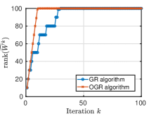
Figure 1: Rank of the matrix $\widehat{W}^{k}$ corresponding to the GR algorithm (blue curve) and OGR algorithm (red curve) for a fully observable system. Both algorithms make use of a basis constructed as in (30).

The rank increases monotonically during the iterations and becomes full after about 30 iterations. However, the curve is not strictly monotonically increasing since the rank does not increase at each iteration. If we repeat the same experiment (with the same matrices) using the OGR Algorithm 3, we obtain the red curve in Figure 1. This curve is strictly monotonically increasing in the first part and becomes constant only once the rank has become full. In particular, at each iteration the rank increases by 10 and the OGR algorithm could be in principle stopped much earlier than the original GR algorithm, and much less control functions (hence laboratory experiments) are needed to fully reconstruct the unknown operator $B^{\star}$. This experiment clearly shows the high potential of the OGR algorithm, which is capable to choose among the elements $B_{1},\dots,B_{K}$ in an optimized fashion.

Let us conclude this section with two important observations. First, the improvement proposed in Algorithm 3 allows one to even enrich the set $(B_{j})_{j=1}^{K}$ used as input in Algorithm 3 with other new elements that can be linearly dependent on $B_{1},\ldots,B_{K}$. In this case, if we denote by $(B_{j})_{j=1}^{\widetilde{K}}$, for $\widetilde{K}>K$, the enriched set, then Theorem 6.1 guarantees that the OGR algorithm will automatically pick some elements of the enriched set $(B_{j})_{j=1}^{\widetilde{K}}$, such that $\mathcal{O}_{N}(C,A)B_{j}$ are linearly independent for all selected $B_{j}$. Hence, the corresponding discriminatory cost-function values will be strictly positive. Second, the OGR Algorithm can be extended to more general nonlinear reconstruction problems, and we propose in Section 6.2 an efficient extension for the Hamiltonian reconstruction problem described in Section 3 at the beginning of this paper.

6.2 Optimized greedy reconstruction for non-linear problems

The extension of the OGR Algorithm 3 to the nonlinear Hamiltonian reconstruction problem of Section 3 is formally rather straightforward and given by Algorithm 4.

Algorithm 4 Optimized Greedy Reconstruction Algorithm (Hamiltonian case)

0:  A set of $K$ matrices $\mathcal{B}_{\mu}=(\mu_{\ell})_{\ell=1,\dots,K}$ and a tolerance tol$>0$.

1:  Solve the initialization problem

(36) $$\max_{n\in\{1,\ldots,K\}}\max_{\epsilon\in L^{2}}|\varphi(\mu_{n},\epsilon)-\varphi(0,0)|^{2}.$$

which gives the field $\epsilon^{1}$ and the index $\ell_{1}$.

2:  if $|\varphi(\mu_{\ell_{1}},\epsilon^{1})-\varphi(0,0)|^{2}<{\rm tol}$ then

3:     stop.

4:  end if

5:  Switch $\mu_{1}$ and $\mu_{\ell_{1}}$ in $\mathcal{B}_{\mu}$ and set $k=1$.

6:  while  $k\leq K-1$  do

7:     for $\ell=k+1,\ldots,K$ do

8:        Fitting step: Find $(\boldsymbol{\alpha}^{\ell}_{j})_{j=1,\dots,k}$ that solve the problem

(37) $$\min\limits_{\boldsymbol{\alpha}\in\mathbb{R}^{k}}\sum_{m=1}^{k}|\varphi(\mu_{k+1},\epsilon^{m})-\varphi(\mu^{k}(\boldsymbol{\alpha}),\epsilon^{m})|^{2}.$$

9:     end for

10:     Extended discriminatory step: Find $\epsilon^{k+1}$ and $\ell_{k+1}$ that solve the problem

(38) $$\max_{\ell\in\{k+1,\ldots,K\}}\max\limits_{\epsilon\in L^{2}}|\varphi(\mu_{k+1},\epsilon)-\varphi(\mu^{k}(\boldsymbol{\alpha}^{k}),\epsilon)|^{2}.$$

11:     if $|\varphi(\mu_{\ell_{k+1}},\epsilon^{k+1})-\varphi(\mu^{k}(\boldsymbol{\alpha}^{\ell_{k}}),\epsilon^{k+1})|^{2}<{\rm tol}$ then

12:        stop and return the selected $(\mu_{j})_{j=1}^{k}$ and the computed $(\epsilon^{m})_{m=1}^{k}$.

13:     end if

14:     Switch $\mu_{k+1}$ and $\mu_{\ell_{k+1}}$ in $\mathcal{B}_{\mu}$ and update $k\leftarrow k+1$.

15:  end while

However, a few more computational aspects must be discussed. First, the maximization problems characterizing the initialization step and the discriminatory steps are nonlinear optimal control problems that we solve numerically by the monotonic scheme discussed in [14]; see also [16, 13, 4, 14] and references therein. Second, the fitting step problems are highly nonlinear minimization problems having generally several local minima. Since not all local minima correspond to an effective defect (rank deficiency in the linear-quadratic case) to be compensated, every fitting-step problem is solved multiple times using different randomly chosen initializations. The solution corresponding to the smallest functional value is then chosen. Each fitting-step problem is solved by a BFGS descent-direction method. Third, all optimization problems that are solved in the fitting steps and in the discriminatory steps are independent one from another. Therefore, they can be solved in parallel as in the linear case.

Let us now show the efficiency of the OGR Algorithm 4 by direct numerical experiments. We consider the same test case as in [13], where the internal Hamiltonian and the unknown (randomly generated) dipole moment matrix are

$$H=10^{-2}\footnotesize\begin{bmatrix}1&0&0\\ 0&2&0\\ 0&0&4\end{bmatrix},\;\mu^{\star}=\footnotesize\begin{bmatrix}3.3617&3.4347&0.8416\\ 3.4347&3.7763&4.7552\\ 0.8416&4.7552&4.4226\\ \end{bmatrix}.$$

The final time is $T=4000\pi$. The states $\psi_{0}$ and $\psi_{1}$ are

$$\psi_{0}=\begin{bmatrix}1&0&0\end{bmatrix}^{\top},\quad\psi_{1}=\begin{bmatrix}0&0&1\end{bmatrix}^{\top}.$$

Now, we perform the following experiment. Since the unknown $\mu^{\star}$ is a $3\times 3$ symmetric matrix, we choose for the set $\mathcal{B}_{\mu}$ the following $K=6$ linearly independent canonical matrices

$$\small\begin{bmatrix}1&0&0\\ 0&0&0\\ 0&0&0\\ \end{bmatrix},\begin{bmatrix}0&0&0\\ 0&1&0\\ 0&0&0\\ \end{bmatrix},\begin{bmatrix}0&0&0\\ 0&0&0\\ 0&0&1\\ \end{bmatrix},\begin{bmatrix}0&1&0\\ 1&0&0\\ 0&0&0\\ \end{bmatrix},\begin{bmatrix}0&0&1\\ 0&0&0\\ 1&0&0\\ \end{bmatrix},\begin{bmatrix}0&0&0\\ 0&0&1\\ 0&1&0\\ \end{bmatrix},$$

which form a basis for ${\rm Sym}(3)$, and compute 6 control functions by the OGR Algorithm 4. Once these functions are obtained, one must reconstruct the unknown true dipole matrix by solving the online nonlinear least-squares problem (2). To do so, we use the standard MATLAB function fminunc (a BFGS descent-direction minimization algorithm) initialized by a randomly chosen vector. To test the robustness of the control functions computed by the OGR Algorithm 4, we consider a six-dimensional hypercube centered in the global minimum point $\boldsymbol{\alpha}^{\star}$ and given radius $r$, and repeat the minimization for 1000 initialization vectors randomly chosen in this hypercube. We then count the number of times that the optimization algorithm converges to the global solution $\mu^{\star}=\mu(\boldsymbol{\alpha}^{\star})$ up to a tolerance of 0.005 (half of the smallest considered radius). Repeating this experiment for different values of the radius $r$ of the hypercube, we obtain the results reported in the first row of Table 1.

Hypercube radius $r$	0.01	0.10	0.25	0.50	0.75	1.00
GR (canonical basis)	23	0	0	0	0	0
GR (random basis)	431	43	15	8	1	0
OGR (extended random basis)	939	923	884	735	627	541

Table 1: Numbers of runs (over 1000) that converged to the true solution $\boldsymbol{\alpha}^{\star}$.

These results show clearly the lack of robustness of the controls generated by the GR algorithm: in only 23 cases over the 1000 runs the minimization converged to the true solution, and this happens only for the smallest radius $r=0.01$ of the hypercube.

Next, to test the effect of the chosen basis $\mathcal{B}_{\mu}$, we repeat the same experiment using 6 randomly chosen linearly independent symmetric matrices $\mu_{\ell}$, $\ell=1,\dots,6$. The obtained results of this second test are shown in the second row of Table 1. These are clearly better, but still very unsatisfactory.

Finally, we repeat the experiment using the OGR Algorithm 4 with a set of 12 matrices, namely the 6 unit basis elements shown above and the 6 linearly independent random matrices chosen for the second experiment. We obtain the results shown in the third row of Table 1. These are now very satisfactory. Even though, the number of times that the optimization algorithm converged to the true solution decays as the radius $r$ increases, in the worst case for $r=1.00$ more than 500 of runs converged to $\boldsymbol{\alpha}^{\star}$. These results show clearly the efficiency of the new proposed OGR algorithm.

7 Conclusions

In this work we provided a novel and detailed convergence analysis for the greedy reconstruction algorithm introduced in [13] for Hamiltonian reconstruction problems in the field of quantum mechanics. The presented convergence analysis has considered linear-quadratic (optimization, least-squares) problems and revealed the strong dependence of the performance of the greedy reconstruction algorithm on the observability properties of the system and on the ansatz of the basis elements used to reconstruct the unknown operator. This allowed us to introduce a precise (and in some sense optimal) choice of the basis elements for the linear case and led to the introduction of an optimized greedy reconstruction algorithm applicable also to the nonlinear Hamiltonian reconstruction problem. Numerical experiments demonstrated the efficiency of the new proposed numerical algorithm.

References

• [1] M. Barrault, Y. Maday, N. C. Nguyen, and A. T. Patera. An “empirical interpolation” method: application to efficient reduced-basis discretization of partial differential equations. Comptes Rendus Mathematique, 339(9):667–672, 2004.
• [2] L. Baudouin and A. Mercado. An inverse problem for Schrödinger equations with discontinuous main coefficient. Appl. Anal., 87(10-11):1145–1165, 2008.
• [3] S. Bonnabel, M. Mirrahimi, and P. Rouchon. Observer-based Hamiltonian identification for quantum systems. Automatica, 45(5):1144 – 1155, 2009.
• [4] A. Borzì, G. Ciaramella, and M. Sprengel. Formulation and Numerical Solution of Quantum Control Problems. SIAM, Philadelphia, PA, 2017.
• [5] J. Coron. Control and Nonlinearity. Mathematical surveys and monographs. American Mathematical Society, 2007.
• [6] A. Donovan and H. Rabitz. Exploring the Hamiltonian inversion landscape. Phys. Chem., 16:15615–15622, 2014.
• [7] Y. Fu and G. Turinici. Quantum Hamiltonian and dipole moment identification in presence of large control perturbations. ESAIM: Contr. Optim. Ca., 23(3):1129–1143, 2017.
• [8] J. M. Geremia and H. Rabitz. Global, nonlinear algorithm for inverting quantum-mechanical observations. Phys. Rev. A, 64:022710, 2001.
• [9] J. M. Geremia and H. Rabitz. Optimal Hamiltonian identification: The synthesis of quantum optimal control and quantum inversion. J. Chem. Phys., 118(12):5369–5382, 2003.
• [10] J. M. Geremia, W. Zhu, and H. Rabitz. Incorporating physical implementation concerns into closed loop quantum control experiments. J. Chem. Phys., 113(24):10841–10848, 2000.
• [11] R. A. Horn and C. R. Johnson. Matrix Analysis. Cambridge University Press, USA, 2nd edition, 2012.
• [12] C. Le Bris, M. Mirrahimi, H. Rabitz, and G. Turinici. Hamiltonian identification for quantum systems: Well posedness and numerical approaches. ESAIM: Contr. Optim. Ca., 13(2):378–395, 2007.
• [13] Y. Maday and J. Salomon. A greedy algorithm for the identification of quantum systems. In Proceedings of the 48th IEEE Conference on Decision and Control, 2009, Held jointly whit the 28th Chinese Control Conference (CDC/CCC 2009), IEEE Conference on Decision and Control, pages 375–379, 2009.
• [14] Y. Maday, J. Salomon, and G. Turinici. Monotonic time-discretized schemes in quantum control. Numer. Math., 103(2):323–338, 2006.
• [15] W. Rudin. Real and Complex Analysis, 3rd Ed. McGraw-Hill, Inc., USA, international edition, 1987.
• [16] Salomon, J. Convergence of the time-discretized monotonic schemes. ESAIM: M2AN, 41(1):77–93, 2007.
• [17] E. D. Sontag. Mathematical Control Theory: Deterministic Finite Dimensional Systems (2Nd Ed.). Springer-Verlag, Berlin, Heidelberg, 1998.
• [18] M. Tadi and H. Rabitz. Explicit method for parameter identification. J. Guid. Control Dyn., 20(3):486–491, 1997.
• [19] L. N. Trefethen and D. Bau. Numerical Linear Algebra. SIAM, 1997.
• [20] Y. Wang, D. Dong, B. Qi, J. Zhang, I. R. Petersen, and H. Yonezawa. A quantum Hamiltonian identification algorithm: Computational complexity and error analysis. IEEE Trans. Autom. Control, 63(5):1388–1403, 2018.
• [21] S. Xue, R. Wu, D. Li, and M. Jiang. A gradient algorithm for Hamiltonian identification of open quantum systems. arXiv preprint - arXiv:1905.09990, 2019.
• [22] J. Zhang and M. Sarovar. Quantum Hamiltonian identification from measurement time traces. Phys. Rev. Lett., 113:080401, 2014.
• [23] W. Zhou, S. Schirmer, E. Gong, H. Xie, and M. Zhang. Identification of markovian open system dynamics for qubit systems. Chinese Sci. Bull., 57(18):2242–2246, 2012.
• [24] W. Zhu and H. Rabitz. Potential surfaces from the inversion of time dependent probability density data. J. Chem. Phys., 111(2):472–480, 1999.