Emergence of Charge Loop Current in Geometrically Frustrated Hubbard Model:
Functional Renormalization Group Study

Abstract

Spontaneous current orders due to odd-parity order parameters attract increasing attention in various strongly correlated metals. Here, we discover a novel spin-fluctuation-driven charge loop current (cLC) mechanism based on the functional renormalization group (fRG) theory. The present mechanism leads to the ferro-cLC order in a simple frustrated chain Hubbard model. The cLC appears between the antiferromagnetic and $d$-wave superconducting ($d$SC) phases. While the microscopic origin of the cLC has a close similarity to that of the $d$SC, the cLC transition temperature $T_{\rm cLC}$ can be higher than the $d$SC one for wide parameter range. Furthermore, we reveal that the ferro cLC order is driven by the strong enhancement of the forward scatterings $g_{2}$ and $g_{4}$ owing to the two dimensionality based on the $g$-ology language. The present study indicates that the cLC can emerge in metals near the magnetic criticality with geometrical frustration

Various exotic symmetry-breaking phenomena are recent central issues in strongly correlated metals. For instance, violation of rotational symmetry, so called the nematic order, has been intensively studied in Fe-based Fernandes ; Fernandes2 ; Chubukov-rev ; Chubukov-AL ; Onari-SCVC ; Onari-FeSe ; Yamakawa-FeSe and cuprate Schultz ; Sachdev ; Sachdev2 ; DHLee-PNAS ; Kivelson-NJP ; Yamakawa-Cu ; Kawaguchi-Cu ; Tsuchiizu-Cu1 ; Tsuchiizu-Cu2 ; Chubukov-Cu superconductors in addition to heavy fermion compounds Ikeda-URu2Si2 ; Tazai-CeB6 . Many kinds of even-parity and time-reversal invariant unconventional order, such as the orbital order Onari-SCVC ; Onari-FeSe ; Yamakawa-FeSe , the $d$-wave bond order Schultz ; Sachdev ; Sachdev2 ; DHLee-PNAS ; Kivelson-NJP ; Yamakawa-Cu ; Kawaguchi-Cu ; Tsuchiizu-Cu1 ; Tsuchiizu-Cu2 and the spin-nematic order Fernandes ; Fernandes2 ; Chubukov-rev ; Chubukov-AL , have been proposed as the candidate for the nematic order. (Bond order is the symmetry breaking in correlated hopping integrals.) Although the microscopic mechanism of the nematicity is still under debate, it is believed that many-body effects beyond the mean-field theory are significant Fernandes ; Fernandes2 ; Chubukov-rev ; Chubukov-AL ; Onari-SCVC ; Onari-FeSe ; Yamakawa-FeSe ; Schultz ; Sachdev ; Sachdev2 ; DHLee-PNAS ; Kivelson-NJP ; Yamakawa-Cu ; Kawaguchi-Cu ; Tsuchiizu-Cu1 ; Tsuchiizu-Cu2 ; Chubukov-Cu ; Ikeda-URu2Si2 ; Tazai-CeB6 .

When the unconventional order violates the parity and/or time-reversal symmetries, more exotic phenomena emerge. For example, the parity-violating bond order induces the spontaneous spin current Nersesyan ; Kontani-sLC . Also, the time-reversal violating order causes the static charge current, which accompanies the internal magnetic field that is measurable experimentally. Various charge-loop-currents (cLCs), like the intra-unit cell cLC Varma1 ; Varma2 and antiferro-cLC Affleck ; Bulut-cLC ; Yokoyama ; TKLee ; Ogata ; FCZhang ; 2leg-gia , have been discussed. In square lattice models, the cLC due to nonzero spin chirality has been studied based on SU(2) gauge theory conical ; orbcurrent . In addition to that, the generalized Hubbard ladder system has been studied by fRG and bosonization gene-ladder1 ; gene-ladder2 .

Recently, a number of experimental evidences for the cLC order have been reported. For instance, in quasi 1D two-leg ladder cuprates, the polarized neutron diffraction (PND) reveal the broken time-reversal symmetry cLC-2leg and conclude that the cLC appears. The cLCs are also reported in cuprates TRSB-neutron1 ; TRSB-neutron2 and iridates TRSB-iridate by PND studies, and their existences are supported by the optical second harmonic generation (SHG) SHG-cuprate ; SHG-iridate , Kerr effect Kerr-cuprate and magnetic torque torque-iridate measurements.

These observations indicate the existence of a universal mechanism of the cLC that is closely related to the magnetic criticality. However, its microscopic origin is still unknown. Based on a simple Hubbard model with on-site Coulomb interaction $U$, mean-field theories fail to explain the cLC. Therefore, off-site Coulomb and Heisenberg interactions have been analyzed Nersesyan ; Bulut-cLC . However, off-site bare interaction is much smaller than $U$ in usual metals. Then, we encounter essential questions; What is the minimum model to understand the cLC ? What is the relation between cLC and magnetic criticality?

In this paper, we propose a novel spin-fluctuation-driven cLC mechanism based on the functional renormalization group (fRG) theory Metzner ; Metzner2 ; Metzner3 ; Honnerkamp ; Honnerkamp2 ; Honnerkamp3 ; Tsuchiizu-RG ; Tsuchiizu2015 ; Tazai-RG ; fRG-lect . Here, we optimize the form factor, which characterizes the essence of the unconventional order, unbiasedly based on the Lagrange multipliers method. By virtue of this method, the ferro-cLC order is obtained without bias in a simple frustrated chain Hubbard model given in Fig. 1(a). We discover that the cLC appears between the antiferromagnetic (AFM) phase and $d$-wave superconducting ($d$SC) phase as schematically shown in Fig. 1(b). The present theory indicates that cLC can emerge in strongly correlated electron systems with geometrical frustration.

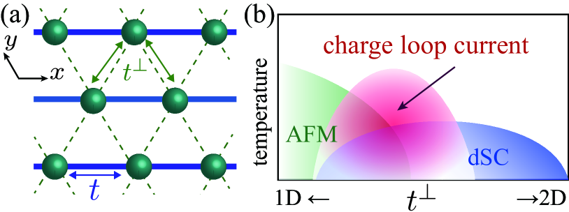
Figure 1: (a) Lattice structure with intra- ($t$) and inter- ($t^{\perp}$) chain hoppings. (b) Schematic phase diagram. The cLC phase appears between AFM and $d$SC phase.

The dimensional crossover in the coupled chain model has been studied intensively for years Emery ; Bourbonnais ; Kishine1 ; Kishine4 ; Suzumura ; Suzumura2 . For $T\gg t^{\perp}$, each Hubbard chain is essentially independent because the thermal de Broglie wavelength is extremely short. For $T\ll t^{\perp}$, inter-chain coherence is established, and therefore quasi two-dimensional Fermi liquid (FL) state with finite quasi-particle weight is realized. In the latter case, one-loop fRG method is very useful since the incommensurate nesting vector of the Fermi surface (FS) is accurately incorporated into the theory. In the $g$-ology language Emery ; Bourbonnais ; Kishine1 ; Kishine4 ; Suzumura ; Suzumura2 ; Solyom , the cLC order in the present theory is caused by the strong renormalization of the forward scatterings $g_{2}$ and $g_{4}$ owing to the two dimensionality.

Here, we study quasi-one-dimensional (q1D) electron systems described by $\hat{H}=\hat{H}_{0}+\hat{H}^{\prime}$. The kinetic term is $\hat{H}_{0}=\sum_{{{\bm{k}}}\sigma}\epsilon_{{{\bm{k}}}}c^{\dagger}_{{{\bm{k}}}\sigma}c_{{{\bm{k}}}\sigma}$ where $c^{\dagger}$ is a creation operator for the electron with the momentum ${{\bm{k}}}$ and spin $\sigma$. The energy dispersion is simply given by $\epsilon_{{{\bm{k}}}}=-2t\cos k_{x}-2t^{\perp}\{\cos k_{y}+\cos(k_{x}+k_{y})\}-\mu$ with $t=1$ and the chemical potential $\mu$. The inter-chain hopping $t^{\perp}(\ll 1)$ controls the dimensionality; $t^{\perp}\rightarrow 0$ corresponds to complete 1D system. We also introduce on-site Coulomb interaction $\hat{H}^{\prime}=\sum_{i}Un_{i\uparrow}n_{i\downarrow}$ where $i$ is the site index.

Now, we perform the fRG method to derive effective low-energy interaction. In the present numerical study, we divide each left-Brillouin zone (BZ) and right-BZ into $24$ patches. The center points of the patches $\bm{p}_{i}$ are shown in Fig. 2(a) and the Supplemental Materials A (SM.A) SM . Here, we introduce logarithmic energy scaling parameter $\Lambda_{l}=\Lambda_{0}e^{-l}(0\leq l\leq l_{c})$ for $\Lambda_{0}=3$, which is slightly larger than $\max_{{{\bm{k}}}}{|\epsilon_{{{\bm{k}}}}|}\simeq 2.8$. In the following numerical study, we consider the half-filling case and put $l_{c}=8.7$ ($\Lambda_{l_{c}}=T/100$) and $U=2.01$ in the unit $t=1$. Also, we fix $(t^{\perp},T)=(0.2,0.05)$ except for the phase diagram in Fig. 3. During the fRG analysis, the low-energy effective interaction changes with the cut off $\Lambda_{l}$. It is represented on the patches as

$$\hat{H}^{\prime}_{\rm{eff}}=\frac{1}{4}{\sum}_{\{p_{i}\}}g_{p_{1}p_{2}p_{3}p_{4}}c^{\dagger}_{p_{1}}c_{p_{2}}c_{p_{3}}c_{p_{4}}^{\dagger},$$ (1)

where $\hat{g}$ is antisymmetric 4-point vertex function with patch ${{\bm{p}}}_{i}$ and spin index where $p_{i}\equiv({{\bm{p}}}_{i},\sigma_{i})$. $\hat{g}$ is defined in Fig. 2(b), and its initial condition is $g_{p_{1}p_{2}p_{3}p_{4}}=U\delta_{{{\bm{p}}}_{1}+{{\bm{p}}}_{4},{{\bm{p}}}_{2}+{{\bm{p}}}_{3}}(\delta_{\sigma_{1},\sigma_{3}}\delta_{\sigma_{2},\sigma_{4}}-\delta_{\sigma_{1},\sigma_{2}}\delta_{\sigma_{3},\sigma_{4}})$. Then, $\hat{g}$ is calculated by solving the 1-loop RG equation,

$$\frac{d}{d\Lambda_{l}}g_{p_{1}p_{2}p_{3}p_{4}} = \sum_{pp^{\prime}}\Bigl{[}\frac{1}{2}\frac{dW_{p,p^{\prime}}^{-}}{d\Lambda_{l}}g_{p_{1}pp^{\prime}p_{4}}g_{pp_{2}p_{3}p^{\prime}}$$ (2)

$$+ \frac{dW_{p,p^{\prime}}^{+}}{d\Lambda_{l}}\Bigl{(}g_{p_{1}p_{3}pp^{\prime}}g_{pp^{\prime}p_{2}p_{4}}-g_{p_{1}p_{2}pp^{\prime}}g_{pp^{\prime}p_{3}p_{4}}\Bigr{)}\Bigr{]},$$

where $W_{p,p^{\prime}}^{\pm}=T\sum_{\bm{k}\bm{k}^{\prime}n}G_{\bm{{{\bm{k}}}}n}G_{\bm{{{\bm{k}}}}^{\prime}\pm n}\Omega_{\bm{p}}(\bm{k})\Omega_{\bm{p}^{\prime}}(\bm{k}^{\prime})$. Here, $G_{\bm{k}n}\equiv(i\epsilon_{n}-\epsilon_{\bm{k}})^{-1}\theta(\Lambda_{l}-|\epsilon_{{{\bm{k}}}}|)$, and $\Omega_{\bm{p}}(\bm{k})=1\ (0)$ only if the momentum $\bm{k}$ is inside (outside) the $\bm{p}$-patch. Here, $\epsilon_{n}$ is fermion Matsubara frequency. The 1st term of r.h.s of the Eq. (2) is the particle-particle loop (=Cooper-channel (ch)), and the 2nd and 3rd terms are the particle-hole loops (=Peierls-ch). Their diagrammatic expressions are in SM.A SM .

Here, we calculate the particle-hole susceptibilities, which are essentially given by the 4-point vertex function in Fig. 2(c). The static charge (spin)-ch susceptibilities with the form factor $f_{{{\bm{k}}}}^{{{\bm{q}}}}$ is defined by

$$\chi^{c(s)}({{\bm{q}}}) = \int^{T^{-1}}_{0}d\tau\frac{1}{2}\left\langle A^{c(s)}({\bm{q}},\tau)A^{c(s)}({\bm{-}{{\bm{q}}}},0)\right\rangle,$$

$$A^{c(s)}({\bm{q}},\tau) \equiv \sum_{\bm{k}\sigma\sigma^{\prime}}\sigma^{0(z)}_{\sigma\sigma^{\prime}}f_{{{\bm{k}}}}^{{{\bm{q}}}}c^{\dagger}_{{{{\bm{k}}}+{{\bm{q}}}}\sigma}(\tau)c_{{{{\bm{k}}}}\sigma^{\prime}}(\tau),$$ (3)

where $\tau$ is imaginary-time. $\hat{\sigma}^{0}$ is identity matrix and $\hat{\sigma}^{z}$ is the Pauli matrix. Here, we optimize the form factor $f_{{{\bm{k}}}}^{{{\bm{q}}}}$ unbiasedly to maximize $\chi^{c}({{\bm{q}}})$ at each ${{\bm{q}}}$-point using the Lagrange multipliers method; see the SM.A SM .

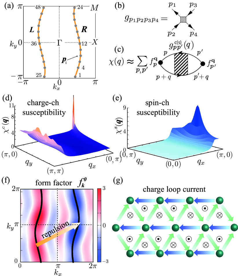
Figure 2: (a) FS with center positions of the patches. (b) 4-point vertex function $\hat{g}$. (c) Susceptibility with the form factor $f^{{{\bm{q}}}}_{{{\bm{p}}}}$. (d) Development of $\chi^{c}({{\bm{q}}})$ at ${{\bm{q}}}=\bm{0}$, which leads to the ferro-cLC. (e) Spin susceptibility with the peak at ${{\bm{q}}}=(\pi,\pi/2)$. (f) Obtained charge-channel form factor $f_{{{\bm{k}}}}^{{{\bm{q}}}=\bm{0}}(\propto\sin k_{x}+b\sin 3k_{x})$. (g) Schematic picture of the cLC.

The form factor corresponds to the modulation of the correlated hopping integral from $j$ to $i$-site, $\delta t_{ij}(i\neq j)$. It is given as $\delta t_{ij}=\Delta t\sum_{{{\bm{k}}}}f_{{{\bm{k}}}}^{{{\bm{q}}}=\bm{0}}e^{i{{\bm{k}}}(\bm{r}_{i}-\bm{r}_{j})}$ for the uniform modulation. Here, both the bond order ($\delta t_{ij}=\delta t_{ji}$) and the cLC ($\delta t_{ij}=-\delta t_{ji}$) are described. Due to the Hermite condition, $\delta t_{ij}$ for the cLC order is pure imaginary. In Figs. 2(d) and (e), we plot the ${{\bm{q}}}$-dependence of the charge- and spin-ch susceptibilities, respectively. The strong charge-ch fluctuations develop at ${{\bm{q}}}=\bm{0}$, while the spin fluctuations remain small even at the peak ${{\bm{q}}}=(\pi,\pi/2)\equiv\bm{Q}_{\rm{AFM}}$. Figure 2(f) shows the charge-ch form factor at ${{\bm{q}}}=\bm{0}$. For a fixed $k_{y}$, the relation $f^{\bm{0}}_{k_{x}}\simeq-f^{\bm{0}}_{-k_{x}}(\propto\sin k_{x}+b\sin 3k_{x})$ holds. Then, the real-space order parameter is $\delta t_{ij}=-\delta t_{ji}$ that leads to the emergence of ferro-cLC order. The third-nearest-intra-chain form factor derived from the present fRG is significant for realizing the cLC SM . In Fig. 2(g), we show the schematic picture of the cLC, which is a magnetic-octupole-toroidal order. The detailed explanation of the numerical results are shown in Fig. S4 in SM.B SM .

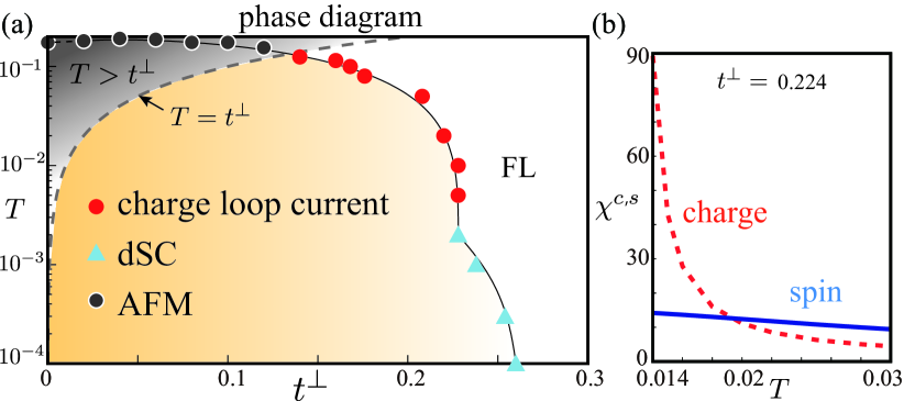
Figure 3: (a) Obtained phase diagram. The cLC appears in the FL regime. (b) Temperature dependence of the susceptibilities for the charge-ch (dotted line) and spin-ch (solid line).

In Fig. 3(a), obtained phase diagram in the $T$-$t^{\perp}$ space is plotted. We reveal that the cLC phase appears around $t^{\perp}\simeq 0.2$ as an intertwined order between AFM and $d$SC states. Note that the dark shaded area is 1D Mott insulating phase that is beyond the scope of the present study Kishine1 ; Kishine4 . In addition, Fig. 3(b) shows the $T$-dependence of the $\chi^{c}(\bm{0})$ and $\chi^{s}(\bm{Q}_{\rm{AFM}})$. $\chi^{c}(\bm{0})$ drastically develops at low temperatures. The transition temperatures in Fig. 3(a) are determined under the condition that the largest susceptibility (spin, charge, $d$SC) exceeds $\chi_{\rm{max}}=30$, while the phase diagram is insensitive to $\chi_{\rm{max}}\ (\gg 10)$, as recognized in Fig. 3(b). As a result, the cLC phase is stabilized in the FL region around $t_{\perp}\gg T$.

To understand the origin of the cLC, we analyze the charge (spin)-ch 4-point vertex function defined by

$$g^{c(s)}_{{{\bm{p}}}{{\bm{p}}}^{\prime}}({{\bm{q}}})\equiv g_{{{\bm{p}}}\uparrow{{\bm{p}}}+{{\bm{q}}}\uparrow{{\bm{p}}}^{\prime}\uparrow{{\bm{p}}}^{\prime}+{{\bm{q}}}\uparrow}+(-)g_{{{\bm{p}}}\uparrow{{\bm{p}}}+{{\bm{q}}}\uparrow{{\bm{p}}}^{\prime}\downarrow{{\bm{p}}}^{\prime}+{{\bm{q}}}\downarrow}.$$ (4)

In Fig. 4(a), we plot the patch-dependence of the charge-ch 4-point vertex $g^{c}_{\bm{pp^{\prime}}}(\bm{0})$. The relation $g^{c}_{\bm{RR^{\prime}}}(\bm{0})\approx-g^{c}_{\bm{LR}}(\bm{0})$ holds, where $\bm{R}=1\sim 24\ (\bm{L}=25\sim 48)$ is patch index in the right (left) branch. We also plot the flow ($l$-dependence) of the 4-point vertex in Fig. 4(b). $g_{\bm{RR^{\prime}}}^{c}(\bm{0})$ comes to be large negative value, while $g_{\bm{LR}}^{c}(\bm{0})$ takes large positive value.

In order to explain why odd-parity form factor is obtained, we introduce $\bar{g}^{c(s)}_{RR}({{\bm{q}}})$, $\bar{g}^{c(s)}_{LR}({{\bm{q}}})$, $\bar{f}^{\bm{0}}_{{R}}$, $\bar{f}^{\bm{0}}_{{L}}$ as their maximum values in the patch space. In this case, the charge-ch susceptibility is

$$\chi^{c}(\bm{0})\propto-(\bar{f}^{\bm{0}}_{{R}})^{2}\bar{g}^{c}_{{RR}}(\bm{0})-\bar{f}^{\bm{0}}_{{L}}\bar{f}^{\bm{0}}_{{R}}\bar{g}^{c}_{{LR}}(\bm{0})$$ (5)

as shown in Fig. 2(c). Since $\bar{g}^{c}_{{RR}}(\bm{0})$ is negative and $\bar{g}^{c}_{{LR}}(\bm{0})$ is positive, the relation $\bar{f}^{\bm{0}}_{{R}}=-\bar{f}^{\bm{0}}_{{L}}$ is required to maximize the susceptibility. In conclusion, the odd-parity cLC appears due the sign reversal between $\bar{g}^{c}_{{RR}}(\bm{0})$ and $\bar{g}^{c}_{{LR}}(\bm{0})$ in the FL region. As for the spin-ch susceptibilities, both $g_{{RR}}^{s}(\bm{Q}_{\rm{AFM}})$ and $g_{{LR}}^{s}(\bm{Q}_{\rm{AFM}})$ are negative, and therefore the spin-ch form factor, does not have any sign reversal on the FS as shown in Fig. S3 in SM.A SM . Thus, ordinal AFM phase is realized in the 1D regime.

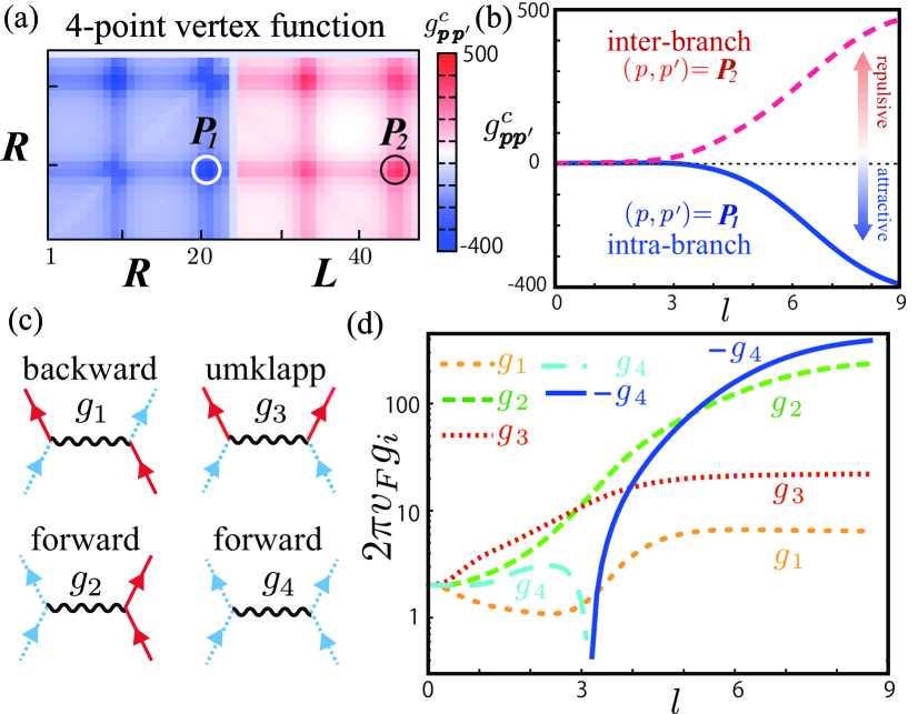
Figure 4: (a) Patch-dependence of four-point vertex at ${{\bm{q}}}=\bm{0}$. The obtained relation $g^{c}_{\bm{RR}}(\bm{0})\approx-g^{c}_{\bm{LR}}(\bm{0})$ gives the ferro-cLC. (b) Flow of $g^{c}_{{{\bm{p}}}{{\bm{p}}}^{\prime}}(\bm{0})$. $g^{c}_{\bm{RR(LR)}}(\bm{0})$ takes large negative (positive) value as the cutoff energy decreases. (c) Definition of the $g_{i}$ in the $g$-ology theory. Dotted (solid) line gives electron on the right (left) branch. (d) Obtained flow of $g_{i}$.

Here, we discuss the present result in terms of the 1D $g$-ology theory Bourbonnais , in which the 4-point vertex function is classified into 4-types; backward ($g_{1}$), forward ($g_{2},g_{4}$) and umklapp ($g_{3}$) scatterings as defined in Fig. 4(c). As an approximation, there is one-to-one correspondence between $\bar{g}_{pp^{\prime}}^{c(s)}({{\bm{q}}})$ and $g_{i}(i=1-4)$ as

$$\!\!\!\!\!\!\bar{g}^{c}_{RR}(\bm{0})\approx 2\pi v_{F}g_{4},\hskip 3.0pt \!\!\!\bar{g}^{c}_{LR}(\bm{0})\approx 2\pi v_{F}(2g_{2}-g_{1}),$$ (6)

$$\!\!\!\!\!\!\bar{g}^{s}_{RR}(\bm{Q}_{\rm{AFM}})\approx-2\pi v_{F}g_{2},\hskip 3.0pt \!\!\!\bar{g}^{s}_{LR}(\bm{Q}_{\rm{AFM}})\approx-2\pi v_{F}g_{3},$$

where $v_{F}$ is the Fermi velocity.

Based on the Eq.(6), we plot the flow of $g_{i}$ in Fig. 4(d). We find that $g_{4}$ ($g_{2}$) has large negative (positive) value as the $l$ increases. The present result is understood by using the knowledge of the $g$-ology theory as we discuss in SM.D SM : At half filling, $g_{2}$ is relevant due to the Peierls-ch scattering Bourbonnais . In the present q1D model, the frustrated hopping $t^{\perp}$ violate the perfect nesting condition, and therefore $g_{2}$ (or AFM fluctuation) is relatively suppressed at $\Lambda_{l}<t^{\perp}$ compared with pure 1D systems Emery ; Bourbonnais ; Kishine1 ; Kishine4 ; Suzumura ; Suzumura2 . On the other hand, surprisingly, $g_{4}$ takes large negative values due to the Landau-ch scattering that is important at low energies ($\Lambda_{l}<T$). As a result, 1D AFM instability is suppressed by $t^{\perp}$, and the cLC due to the Landau-ch instead appears. (Importance of the $g_{4}$ on $\chi^{s}(\bm{0})$ was discussed in Ref. fuseya_g4 .) Thus, the geometrical frustration is essential for realizing the cLC order.

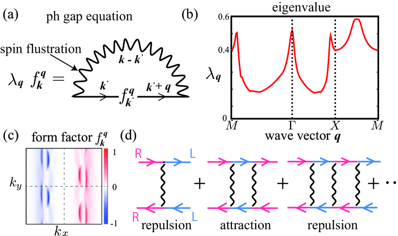
Figure 5: (a) The ph gap equation. Wavy line is spin fluctuations given by the RPA. (b) Obtained eigenvalue of the gap equation at $(T,U)=(0.03,1.65)$. The peak around $\Gamma$-point corresponds to the cLC. (c) Obtained charge-ch form factor at ${{\bm{q}}}=\bm{0}$, which is essentially the same as the fRG results. (d) Dominant contribution for stabilizing the cLC order.

Also, the cLC is naturally understood by the spin-fluctuation-driven mechanism based on 2D FL concept Kontani-rev ; Moriya ; Yamada . To show this, we solve the ”particle-hole (ph) gap equation” for charge-ch form factor $f^{{{\bm{q}}}}_{{{\bm{k}}}}$ ;

$$\lambda_{{{\bm{q}}}}f^{{{\bm{q}}}}_{{{\bm{k}}}}=\sum_{{{\bm{k}}}^{\prime}}f^{{{\bm{q}}}}_{{{\bm{k}}}^{\prime}}L({{\bm{k}}}^{\prime},{{\bm{q}}})\left(-\frac{3}{2}V^{s}_{{{\bm{k}}}-{{\bm{k}}}^{\prime}}-\frac{1}{2}V^{c}_{{{\bm{k}}}-{{\bm{k}}}^{\prime}}\right),$$ (7)

where $\lambda_{{{\bm{q}}}}$ is the eigenvalue. Here, we define $V^{c(s)}_{{{\bm{q}}}}\equiv-(+)U+U^{2}\chi^{c(s)}({{\bm{q}}})$ in the random-phase approximation (RPA), and $L({{\bm{k}}},{{\bm{q}}})\equiv(n_{{{\bm{k}}}-\frac{{{\bm{q}}}}{2}}-n_{{{\bm{k}}}+\frac{{{\bm{q}}}}{2}})/(\epsilon_{{{\bm{k}}}+\frac{{{\bm{q}}}}{2}}-\epsilon_{{{\bm{k}}}-\frac{{{\bm{q}}}}{2}})>0$ with Fermi distribution function $n_{{{\bm{k}}}}$. The diagrammatic expression of the ph gap equation in Fig. 5(a) is given by the 1st order spin fluctuation exchange term ($=$MT-type process). Figure 5(b) shows the largest eigenvalue $\lambda_{{{\bm{q}}}}$ for general ${{\bm{q}}}$. The 2nd largest peak at $\Gamma$-point corresponds to the cLC since the obtained odd-parity form factor in Fig. 5(c) is essentially the same as the results by the fRG. (Obviously, the fRG method is superior to RPA in that loop cancellation in 1D system is taken into account.) Figure 5(d) shows the scattering processes generated by solving the ph gap equation. The even (odd)-order processes with respect to $\chi^{s}(\bm{Q}_{\rm AFM})$ work as inter-branch repulsion (intra-branch attraction), and it corresponds to $\bar{g}^{c}_{{RR}}<0\ (\bar{g}^{c}_{{LR}}>0)$ in Fig.4 (a). Thus, the cLC is naturally explained in terms of the FL concept, and this mechanism is found to be similar to that for the $d$SC near the AFM phase Kishine1 ; Kishine4 ; Suzumura ; Suzumura2 ; Kino .

Furthermore, we perform the fRG without Cooper-ch processes and confirm that the cLC is obtained even if we neglect the Cooper-ch as shown in Fig. S5 in SM.C SM . Thus, we conclude that the cLC emerges due to the spin-fluctuation-driven mechanism.

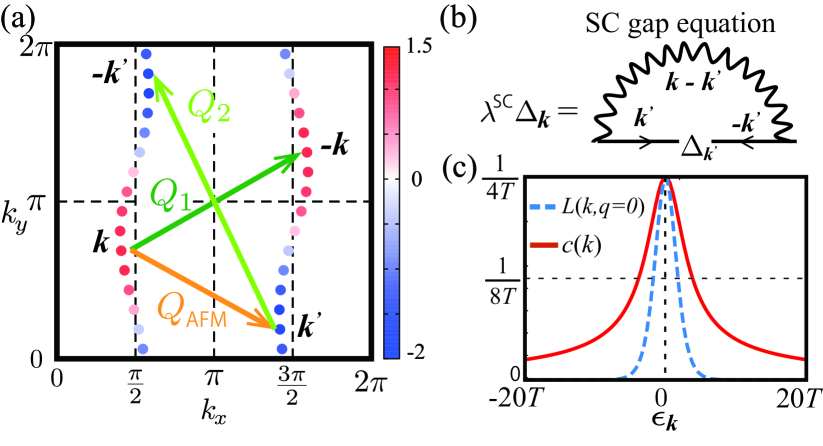
Figure 6: (a) $d$SC gap function obtained by the fRG. (b) SC gap equation. (c) $\epsilon_{{{\bm{k}}}}$-dependence of $L({{\bm{k}}},{{\bm{q}}}=0)$ and $C({{\bm{k}}})$.

Next, we discuss the $d$SC phase. Figure 6(a) shows the optimized SC gap given by the fRG Tsuchiizu-Cu1 . This $d$SC gap is well understood in terms of the singlet SC gap equation with the MT-process Kino ;

$$\lambda^{SC}\Delta_{{{\bm{k}}}}=\sum_{{{\bm{k}}}^{\prime}}\Delta_{{{\bm{k}}}^{\prime}}C({{\bm{k}}}^{\prime})\left(-\frac{3}{2}V^{s}_{{{\bm{k}}}-{{\bm{k}}}^{\prime}}+\frac{1}{2}V^{c}_{{{\bm{k}}}-{{\bm{k}}}^{\prime}}\right),$$ (8)

where $C({{\bm{k}}})=(2n_{{{\bm{k}}}}-1)/(2\epsilon_{{{\bm{k}}}})>0$ and its diagrammatic expression is in Fig. 6(b). Since $\Delta_{{{\bm{k}}}}$ is even-parity, the inter-branch repulsion by $V^{s}_{\bm{Q}_{\rm{AFM}}}$ induce the nodal $d$SC.

Furthermore, we discuss the reason why the cLC phase dominates over the SC phase. As shown in Fig. 6(c), $C({{\bm{k}}})$ in Eq. (8) is always larger than $L({{\bm{k}}},{{\bm{q}}}=\bm{0})$ in Eq. (7) except at $\epsilon_{{{\bm{k}}}}=0$, reflecting the logarithmic Cooper-ch singularity Bourbonnais . On the other hand, the Cooper instability is reduced by the intra-branch sign reversal in the $d$SC gap. By considering the dominant contribution of the gap function at $({{\bm{k}}},{{\bm{k}}}^{\prime},-{{\bm{k}}},-{{\bm{k}}}^{\prime})$ in Fig. 6 (a), the effective pairing interaction for the $d$-wave gap is

$$V_{dSC}\propto\{2\chi^{s}(\bm{Q}_{\rm AFM})-\chi^{s}(\bm{Q}_{1})-\chi^{s}(\bm{Q}_{2})\}\propto(t^{\perp}/t)^{2}.$$ (9)

Thus, the $d$-wave Cooper instability is suppressed by the factor $(t^{\perp}/t)^{2}\ll 1$ due to the 1D nature.

If we consider off-site Coulomb interaction $V$ in addition to $U$, the cLC instability should be enhanced. In fact, the Fock term $-2V\cos({{\bm{k}}}-{{\bm{k}}}^{\prime})$ is added to $V^{c}_{{{\bm{k}}}-{{\bm{k}}}^{\prime}}$ in Eq. (7), and it gives the inter-branch repulsive and intra-branch attractive interactions Varma1 ; Varma2 ; Bulut-cLC ; Nersesyan . Thus, both the spin fluctuation and finite off-site Coulomb $V$ will cooperatively stabilize the cLC phase.

In summary, we proposed the spin-fluctuation-driven cLC mechanism based on the fRG theory. We derived the optimized form factor, which is the key essence of the unconventional order, without any assumptions. By virtue of this method, the ferro-cLC order is obtained without any bias in a simple frustrated chain Hubbard model. For the microscopic origin of the cLC, strong renormalization of the forward scatterings ($g_{2}$,$g_{4}$) due to spin fluctuations plays an important role. We stress that the cLC phase in the FL regions is replaced with the AFM phase if we remove the frustration as shown in Fig. S9 in SM. E. The role of geometrical frustration is to realize strong short-range spin fluctuations that mediate the cLC order. Thus, it will be useful to verify the theoretically predicted correlation between the cLC order and spin fluctuation strength in future experiments.

We are grateful to S. Onari and M. Tsuchiizu for useful discussions. This work is supported by Grants-in-Aid for Scientific Research (KAKENHI) Research (No. JP20K22328, No. JP20K03858, No. JP19H05825, No. JP18H01175) from MEXT of Japan.

[Supplementary Material]
Emergence of Charge Loop Current in Geometrically Frustrated Hubbard Model:
Functional Renormalization Group Study

Rina Tazai, Youichi Yamakawa and Hiroshi Kontani

Department of Physics, Nagoya University, Nagoya 464-8602, Japan

I.1 A. fRG analysis, Optimization of form factor

Here, we present the detailed explanation of the present fRG method. In the framework of the patch-fRG, the ${{\bm{k}}}$-space in the 1st BZ is divided into $N_{p}$-patches. In the present model, we set $N_{p}=48$, and the boundary lines at $\Lambda_{l}=\pm 1$ are shown in Fig. S1. Each patch is rectangular along $k_{x}$-axis.

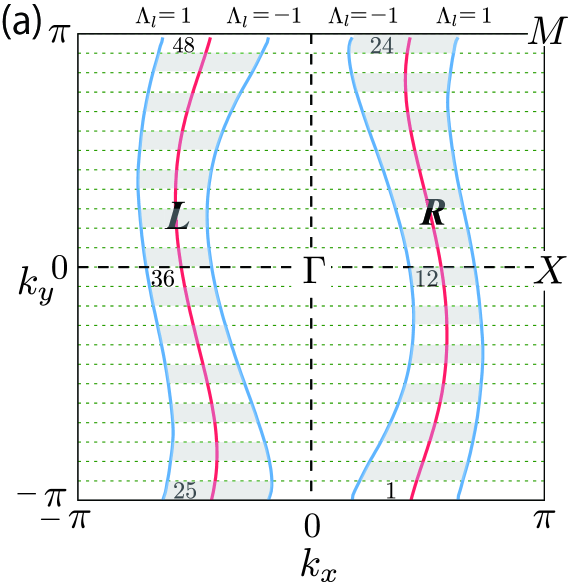
Figure S1: The 48-patches in the 1st BZ. The red (blue) line shows the Fermi surface (boundary line at $\Lambda_{l}=\pm 1$).

Then, we solve the RG equation for the 4-point vertex function $\hat{g}$, which is given in Eq. (2) in the main text. Its diagrammatic expression is in Fig. S2(a). The 1st (2nd and 3rd) term of the r.h.s correspond to the Cooper (Peierls)-ch scattering. After that, the particle-hole susceptibilities are obtained by solving the RG equation,

$$\frac{d\chi^{c(s)}({{\bm{q}}})}{d\Lambda_{l}}=T\sum_{{{\bm{p}}}}\frac{dW^{+}_{{{\bm{p}}},{{\bm{p}}}+{{\bm{q}}}}}{d\Lambda_{l}}R^{c(s)}_{{{\bm{q}}},{{\bm{p}}}}R^{c(s)}_{-{{\bm{q}}},{{\bm{p}}}},$$ (S1)

where $R^{c(s)}$ is the charge (spin)-ch 3-point vertex function and obtained by

$$\frac{dR^{c(s)}_{{{\bm{q}}},{{\bm{p}}}}}{d\Lambda_{l}}=-T\sum_{{{\bm{p}}}^{\prime}}\frac{dW^{+}_{{{\bm{p}}}^{\prime},{{\bm{p}}}^{\prime}+{{\bm{q}}}}}{d\Lambda_{l}}R^{c(s)}_{{{\bm{q}}},{{\bm{p}}}^{\prime}}g^{c(s)}_{{{\bm{p}}}^{\prime}+{{\bm{q}}},{{\bm{p}}}}({{\bm{q}}}),$$ (S2)

where $R^{c(s)}_{{{\bm{q}}},{{\bm{p}}}}$ includes the form factor and $W^{+}_{{{\bm{p}}},{{\bm{p}}}+{{\bm{q}}}}$ is introduced in the main text. The diagrammatic expression of Eqs. (S1) and (S2) are given in Figs. S2(b) and (c), respectively. Thus, the ph susceptibilities are essentially derived from the 4-point vertex function as shown in Fig. 2(c) in the main text.

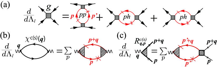
Figure S2: (a) RG equation for the 4-point vertex $\hat{g}$ and that for the (b) charge (spin)-ch susceptibility $\chi^{c(s)}({{\bm{q}}})$ and (c) the 3-point vertex $R^{c(s)}_{{{\bm{q}}},{{\bm{p}}}}$.

Here, we optimize the form factor $f_{{{\bm{k}}}}^{{{\bm{q}}}}$ so as to maximize the ph susceptibility under the constraint $\sum_{{{\bm{k}}}}|f^{{{\bm{q}}}}_{{{\bm{k}}}}|^{2}=1$ at each ${{\bm{q}}}$-point. For this purpose, we introduce the Fourier expansion form of $f^{{{\bm{q}}}}_{{{\bm{k}}}}$ as

$$f_{{{\bm{k}}}}^{{{\bm{q}}}}=\sum_{n,m=1}^{7}a_{nm}^{{{\bm{q}}}}h_{n}(k_{x})h_{m}(k_{y}),$$ (S3)

where $\frac{h_{n}(k)}{\sqrt{2}}=\{\frac{1}{\sqrt{2}},\cos k,\cos 2k,\cos 3k,\sin k,\sin 2k,\sin 3k\}$ for $n=1,2,3,4,5,6,7$, respectively.

Based on the Lagrange multipliers method, the coefficient $a_{M}^{{{\bm{q}}}}$ is optimized under the condition $\frac{1}{N}\sum_{{\bm{k}}}|f_{{{\bm{k}}}}^{{{\bm{q}}}}|^{2}=1$ by solving the following eigen equation,

$$\sum_{M}\chi_{LM}^{c(s)}({{\bm{q}}})a^{{{\bm{q}}}}_{M}=\lambda a_{L}^{{{\bm{q}}}},$$ (S4)

where the index $L\equiv(n,m)$ takes $1-49$. The eigenvale $\lambda$ corresponds to the undetermined multiplier in the Lagrange multipliers method. $\chi_{LM}^{c(s)}({{\bm{q}}})$ is the $(L,M)$ component of the charge-ch (spin-ch) susceptbility calculated by the fRG method:

$$\chi^{c(s)}_{LM}({{\bm{q}}}) \equiv \int^{\beta}_{0}d\tau\frac{1}{2}\left\langle B^{c(s)}_{L}({\bm{q}},\tau)B^{c(s)}_{M}({\bm{-}{{\bm{q}}}},0)\right\rangle,$$

$$B^{c(s)}_{nm}({\bm{q}},\tau) \equiv \sum_{\bm{k}\sigma\sigma^{\prime}}\sigma^{0(z)}_{\sigma\sigma^{\prime}}h_{n}(k_{x})h_{m}(k_{y})c^{\dagger}_{{{{\bm{k}}}+{{\bm{q}}}}\sigma}(\tau)c_{{{{\bm{k}}}}\sigma^{\prime}}(\tau).$$

Note that conventional charge (spin) susceptibility with $f_{{\bm{k}}}^{{\bm{q}}}=1$ is given by $L=M=(1,1)$.

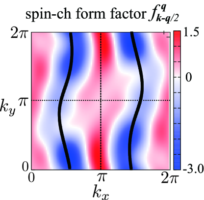
Figure S3: ${{\bm{k}}}$-dependence of the spin-ch form factor, which corresponds to the conventional AFM fluctuation.

In the main text, we show the optimized susceptibilities and its form factor only for the charge-ch. Here, we show the results for the spin-ch. In Fig. S3, we plot spin-ch form factor $f^{{{\bm{q}}}}_{{{\bm{k}}}-{{\bm{q}}}/2}$ for ${{\bm{q}}}=\bm{Q}_{\rm{AFM}}$. It does not have any sign reversal on the FS and the conventional AFM fluctuations develop. Thus, the obtained phase diagram in Fig. 3(a) will be changed only slightly even if we consider the ${{\bm{k}}}$-dependent spin-ch form factor, although the AFM phase will be slightly enhanced.

I.2 B. Charge currents in real space

Now, we show the detailed results of the cLC from $0$-site to $i$-site ($\bm{r}=\bm{0}$), which is defined by SKontani-sLC ,

$$j_{i}\equiv 2ie\left\{(t_{i0}+\delta t_{i0})G(-\bm{r}_{i})-(t_{0i}+\delta t_{0i})G(\bm{r}_{i})\right\},$$ (S5)

where $-e$ is the charge of electron and $\delta t_{i0}$ is obtained by Fourier transformation of charge-ch $f^{{{\bm{q}}}}_{{{\bm{k}}}}$ multiplied by the energy scale $\Delta t$. Note that $\delta t_{i0}$ is pure imaginary and $\delta t_{i0}=-\delta t_{0i}$ holds. Here, equal-time Green function $G(\bm{r}_{i})$ in real space is defined by

$$G(\bm{r}_{i})=T\sum_{n,{{\bm{k}}}}\frac{1}{i\epsilon_{n}-\epsilon_{{{\bm{k}}}}-\Delta tf_{{{\bm{k}}}}^{\bm{0}}}e^{i{{\bm{k}}}\bm{r}_{i}}.$$ (S6)

Figures S4(a) and (b) show the obtained values of the intra- and inter-chain components of the cLC, respectively. Here, we put $e=1$ and $\Delta t=0.05$. The total intra-chain current is $j_{intra}=\sum_{x\geq 1}j(x,0)\times|x|\sim-7\times 10^{-3}$. The schematic current pattern between the nearest sites is given in Fig. 2(g). The cLC-induced magnetic field can be detected by experiments such as NMR. We verified that the macroscopic current is zero due to the cancellation between intra- and inter-chain current. These results are consistent with the ”Bloch’s theory” that proved the absence of the macroscopic currents in the infinite periodic systems SBohm .

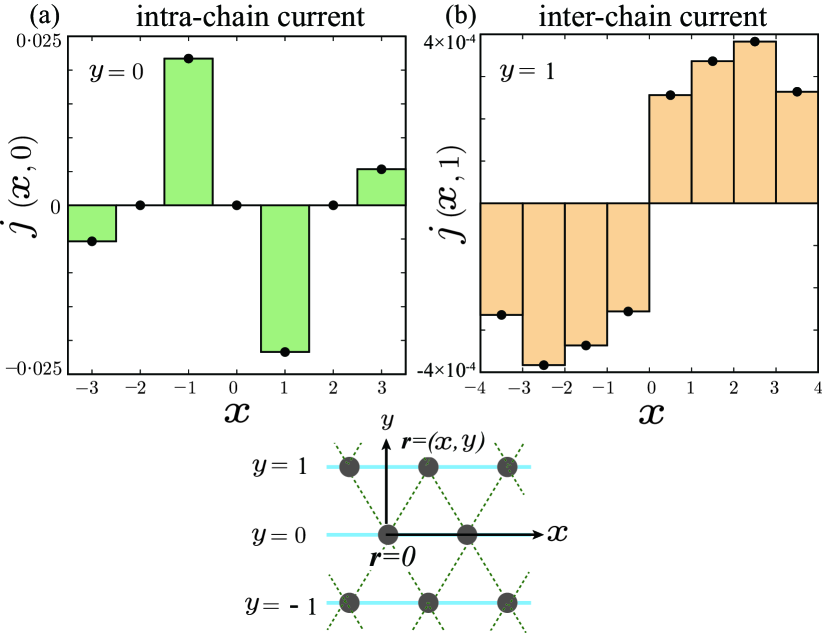
Figure S4: (a) Site-dependence of the intra-chain current $j_{x,y=0}$ and (b) that of inter-chain current $j_{x,y=1}$.

I.3 C. Analysis of the fRG without Cooper-ch

In the main text, we explain that the Peierls-ch scatterings give the dominant contribution to the cLC, while both Peierls- and Cooper-ch scatterings are taken into account on an equal footing in the fRG method. To verify the important of the Peierls-ch for the cLC, we solve the RG equation without Cooper-ch, which is given by

$$\frac{dg_{p_{1}p_{2}p_{3}p_{4}}}{d\Lambda_{l}}=\sum_{pp^{\prime}}\frac{dW_{\bm{p,p^{\prime}}}^{+}}{d\Lambda_{l}}\Bigl{(}g_{p_{1}p_{3}pp^{\prime}}g_{pp^{\prime}p_{2}p_{4}}-g_{p_{1}p_{2}pp^{\prime}}g_{pp^{\prime}p_{3}p_{4}}\Bigr{)}.$$

In Fig. S5, we plot the maximum value of the charge (spin)-ch susceptibilities $\chi^{c(s)}(\equiv\max_{{{\bm{q}}}}\chi^{c(s)}({{\bm{q}}}))$ without Cooper-ch contribution. The charge-ch fluctuations develop at ${{\bm{q}}}=\bm{0}$ even if we drop the Cooper-ch. The obtained result is quite similar as the one in the main text with Cooper-ch as shown in Fig.3 (b). Therefore, we conclude that particle-hole (AFM) fluctuations play a significant role on the microscopic mechanism of the cLC, while the $d$SC fluctuations are irrelevant.

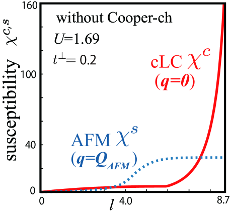
Figure S5: Flows of the charge- and spin-ch susceptibilities without contribution from the Cooper-ch scattering. here, $U=1.69,t^{\perp}$ and $T=0.05$.

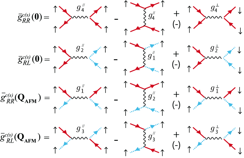
Figure S6: One-to-one correspondence between $\bar{g}_{pp^{\prime}}^{c(s)}({{\bm{q}}})$ and $g_{i}$.

I.4 D. $g$-ology theory at finite temperatures

Here, we summarize the $g$-ology analysis for the cLC on the present q1D Hubbard model with linear energy dispersion.

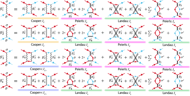
Figure S7: The RG equation for the 4-point vertex $g_{i}$ in the 1-loop approximation.

In the $g$-ology theory SEmery ; SBourbonnais ; SKishine1 ; SKishine4 ; SSuzumura ; SSuzumura2 ; SSolyom , the 4-point vertex function is classified into 4-types; backward ($g_{1}$), forward ($g_{2},g_{4}$) and umklapp ($g_{3}$) scatterings, which are defined in Fig. 4(c) in the main text. By using the $g_{i}(i=1-4)$, the charge- (spin-) ch 4-point vertex $\bar{g}^{c}_{p,p^{\prime}}(\bm{0})$ in the q1D model is given by

$$\!\!\!\!\!\!\bar{g}^{c}_{RR}(\bm{0})\approx 2\pi v_{F}g_{4},\hskip 3.0pt \!\!\!\bar{g}^{c}_{LR}(\bm{0})\approx 2\pi v_{F}(2g_{2}-g_{1})$$ (S7)

$$\!\!\!\!\!\!\bar{g}^{s}_{RR}(\bm{Q}_{\rm{AFM}})\approx-2\pi v_{F}g_{2},\hskip 3.0pt \!\!\!\bar{g}^{s}_{LR}(\bm{Q}_{\rm{AFM}})\approx-2\pi v_{F}g_{3},$$

where its derivation is given in Fig. S6. Based on these relations, we discuss the origin of the cLC in terms of the $g$-ology theory in the main text. The results of the present study are given in the TABLE I.

$\hat{g}$ in q1D	$g$-ology	initial	present study
$\bar{g}^{c}_{{RR}}(\bm{0})$	$2\pi v_{F}\cdot g_{4}$	$U$	large negative
$\bar{g}^{c}_{{LR}}(\bm{0})$	$2\pi v_{F}(2g_{2}-g_{1})$	$U$	large positive
$-\bar{g}^{s}_{{RR}}(\bm{Q}_{\rm AFM})$	$2\pi v_{F}\cdot g_{2}$	$U$	large positive
$-\bar{g}^{s}_{{LR}}(\bm{Q}_{\rm AFM})$	$2\pi v_{F}\cdot g_{3}$	$U$	positive

Table 1: (1st column) The charge- and spin-ch 4-point vertexes, (2nd column) $g_{i}$ in the $g$-ology theory, (3rd column) initial value, (4th column) the present results.

The most important fact is that $g_{2}$ ($g_{4}$) is renormalized to large positive (negative) value in the present q1D model as given in Fig. 4(d) in the main text. To understand the large positive (negative) value of $g_{2}\ (g_{4})$, we consider the 1-loop RG equation for $g_{i}$. We note that $g_{i}$ has spin dependence and is classified into 2-ch in the spin-conserving system: $g_{i}^{\perp}$ and $g_{i}^{\parallel}$. $g_{i}^{\perp}$ is the interaction between fermions with the anti-parallel spin, while $g_{i}^{\parallel}$ is that with the same spin. By using the $g_{i}^{\perp}$ and $g_{i}^{\parallel}$, the RG equation is given by

$$\frac{dg_{1}^{\perp}}{dl} = 2g_{1}^{\perp}g_{2}^{\perp}I_{C}+2g_{1}^{\perp}(g_{2}^{\parallel}-g_{1}^{\parallel})I_{P}+2g_{1}^{\perp}g_{4}^{\perp}I_{L},$$

$$\frac{dg_{2}^{\perp}}{dl} = (g_{2}^{\perp}g_{2}^{\perp}+g_{1}^{\perp}g_{1}^{\perp})I_{C}+2g_{4}^{\perp}(g_{1}^{\parallel}-g_{2}^{\parallel})I_{L}$$

$$+ (g_{2}^{\perp}g_{2}^{\perp}+g_{3}^{\perp}g_{3}^{\perp})I_{P},$$

$$\frac{dg_{3}^{\perp}}{dl} = 2g_{3}^{\perp}g_{4}^{\perp}I_{C+}+2g_{3}^{\perp}(g_{2}^{\parallel}-g_{1}^{\parallel})I_{P}+2g_{3}^{\perp}g_{2}^{\perp}I_{P},$$

$$\frac{dg_{4}^{\perp}}{dl} = (g_{4}^{\perp}g_{4}^{\perp}+g_{3}^{\perp}g_{3}^{\perp})I_{C+}$$ (S8)

$$+ 2g_{2}^{\perp}(g_{1}^{\parallel}-g_{2}^{\parallel})I_{L}+(g_{4}^{\perp}g_{4}^{\perp}+g_{1}^{\perp}g_{1}^{\perp})I_{L}.$$

Their diagrammatic expressions are given in Fig. S7.

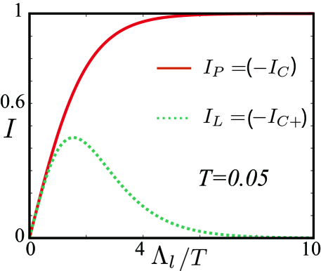
Figure S8: $\Lambda_{l}$-dependence of the $I_{P}=-I_{C}=\tanh(\Lambda_{l}/2T)$ (red solid line) and $I_{L}=-I_{C+}=(\Lambda_{l}/2T)\cosh^{-2}(\Lambda_{l}/2T)$ (green dotted line).

Here, $I_{P}\ (I_{L})$ corresponds to the Peierls (Landau) ch scatterings defined by $I_{P}\ (I_{L})\equiv 2\pi v_{F}\cdot dW_{\bm{R},\bm{L}(\bm{R},\bm{R})}^{+}/dl$. On the other hand, $I_{C(C+)}$ is the Cooper (Cooper+) ch ones where $I_{C}\ (I_{C+})\equiv 2\pi v_{F}\cdot dW_{\bm{R},\bm{L}(\bm{R},\bm{R})}^{-}/dl$.

At finite temperatures, The $\Lambda_{l}/T$-dependence of $I_{P}=-I_{C}$ and $I_{L}=-I_{C+}$ in the linear dispersion model are shown in Fig. S8. (At $T=0$, $I_{P}=-I_{C}=1$ and $I_{L}=I_{C+}=0$.) The Landau-ch scattering plays important roles in the lower energy region comparable to Cooper-ch (Peierls-ch) scattering Sfuseya_g4 . Note that $I_{L}=2\Lambda_{l}[L({{\bm{k}}},{{\bm{q}}}=\bm{0})]_{{\epsilon}_{{\bm{k}}}=\Lambda_{l}}$ and $I_{C}=-2\Lambda_{l}[C({{\bm{k}}})]_{{\epsilon}_{{\bm{k}}}=\Lambda_{l}}$ in Fig. 6(c) in the main text. We comment that the Landau and Cooper+ channels are completely dropped if we set $T=0$ before solving the RG equation. In this case, $g_{4}$ is marginal since $dg_{4}/dl=0$. Therefore, we have to solve the RG equation at finite $T$, and then we can take the $T\rightarrow 0$ limit at the final stage.

By using the SU(2)-symmetry in the spin space, the relation $g_{1}^{\perp}-g_{2}^{\perp}=g_{1}^{\parallel}-g_{2}^{\parallel}$ holds. Thus, all of the $g^{\parallel}$ terms in Eq.(S8) are replaced by $g^{\perp}$. Note that the $g^{\parallel}_{3}$ and $g^{\parallel}_{4}$ does not affect the physical quantity due to the anti-commutation relation of the fermion. Thus, the expression $g_{i}$ in the main text stands for $g_{i}^{\perp}$. In addition, the Cooper-ch scattering is negligible as discussed in SM. C. Then, the RG equations for $g_{2}$ and $g_{4}$ are simply rewritten as

$$\frac{dg_{2}}{dl} = (g^{2}_{2}+g^{2}_{3})I_{P}+(-2g_{2}g_{4}+2g_{1}g_{4})I_{L},$$

$$\frac{dg_{4}}{dl} = (g^{2}_{4}+g^{2}_{1}-2g^{2}_{2}+2g_{1}g_{2})I_{L},$$ (S9)

where we put $g_{i}\equiv g_{i}^{\perp}$. Therefore, $g_{2}$ is enhanced by the Peierls-ch scattering by $(g^{2}_{2}+g^{2}_{3})I_{P}$, while it is suppressed by $-2g_{2}g_{4}I_{L}$. (Note that $g_{1}$ is marginally irrelevant.) On the other hand, $g_{4}$ is renormalized by the Landau-ch scattering. In particular, $g_{4}$ becomes negative value due to the factor $-2g^{2}_{2}I_{L}$. Therefore, we conclude that the cLC is understood by the important roles of $g_{2}$ and $g_{4}$, which are renormalized by Peierls- and Landau-ch scatterings, respectively.

I.5 E. Analysis of the fRG without frustration

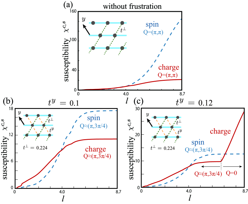
Figure S9: (a) Flows of the maximum values for the charge- and spin-ch susceptibilities without the geometrical frustration at $t^{y}=0$, $U=1.56$ and $\bm{Q}=(\pi,\pi)$. We also show the flows with the weak geometrical frustration at (b) $t^{y}=0.1$ and (c) $t^{y}=0.12$.

Here, we discuss the importance of the magnetic frustration for the emergence of the cLC. For this purpose, we perform the fRG on a coupled Hubbard chain model without frustration, which is realized by cutting the hopping along the $y$-axis; $t^{y}$. Figure S9 (a) shows the obtained charge- and spin-ch susceptibilities at $U=1.56,t^{y}=0,t^{\perp}=0.224$. The value of $U$ is slightly smaller than that in the main text by reflecting the absence of the magnetic frustration. Only spin-ch fluctuations develop at $\bm{Q}=(\pi,\pi)$ while the charge-ch fluctuations remain small. Here, the charge-ch fluctuations correspond to the bond-order at $\bm{Q}=(\pi,\pi)$. The present AFM phase is located in the FL region, since the magnetic transition temperature is $T=0.05\ll t^{\perp}$.

Therefore, the cLC does not appear without the magnetic frustration even in the FL region. We verified that the cLC order can overcome the AFM order for $t^{y}/t^{\perp}\gtrsim 0.5$ for $t^{\perp}=0.224$ at $T=0.05$ as shown in Figs. S9 (b) and (c).

In summary, the geometry frustration strongly suppresses the AFM susceptibility. On the other hand, the AFM fluctuation is important in the present cLC mechanism. Thus, it is useful to verify the correlation between the cLC order and spin fluctuation strength experimentally in order to discriminate the present cLC mechanism from the other cLC ones. Thus, it is possible to discriminate the true cLC mechanism by performing careful multiple experiments. This fact brings a change to develop the Landau-ch scattering that is the origin of the cLC. Therefore, we conclude that the magnetic frustrations are essential ingredient to obtain the cLC in the main text.

References

- (1) R. M. Fernandes, L. H. VanBebber, S. Bhattacharya, P. Chandra, V. Keppens, D. Mandrus, M. A. McGuire, B. C. Sales, A. S. Sefat, and J. Schmalian, Phys. Rev. Lett. 105, 157003 (2010).
- (2) R. M. Fernandes, A. V. Chubukov, J. Knolle, I. Eremin, and J. Schmalian, Phys. Rev. B 85, 024534 (2012)
- (3) A. V. Chubukov, M. Khodas, and R. M. Fernandes, Phys. Rev. X 6, 041045 (2016).
- (4) R.-Q. Xing, L. Classen, and A. V. Chubukov, Phys. Rev. B 98, 041108(R) (2018).
- (5) S. Onari and H. Kontani, Phys. Rev. Lett. 109, 137001 (2012).
- (6) S. Onari, Y. Yamakawa, and H. Kontani, Phys. Rev. Lett. 116, 227001 (2016).
- (7) Y. Yamakawa, S. Onari, and H. Kontani, Phys. Rev. X 6, 021032 (2016).
- (8) H. J. Schulz, Phys. Rev. B 39, 2940(R) (1989).
- (9) M.A. Metlitski and S. Sachdev, New J. Phys. 12, 105007 (2010).
- (10) S. Sachdev and R. La Placa, Phys. Rev. Lett. 111, 027202 (2013).
- (11) J. C. S. Davis and D.-H. Lee, Proc. Natl. Acad. Sci. USA, 110, 17623 (2013).
- (12) E. Berg, E. Fradkin, S. A. Kivelson, and J. M. Tranquada, New J. Phys. 11, 115004 (2009).
- (13) Y. Yamakawa, and H. Kontani, Phys. Rev. Lett. 114, 257001 (2015).
- (14) K. Kawaguchi, Y. Yamakawa, M. Tsuchiizu, and H. Kontani, J. Phys. Soc. Jpn. 86, 063707 (2017).
- (15) M. Tsuchiizu, Y. Yamakawa, and H. Kontani, Phys. Rev. B 93, 155148 (2016).
- (16) M. Tsuchiizu, K. Kawaguchi, Y. Yamakawa, and H. Kontani, Phys. Rev. B 97, 165131 (2018).
- (17) Y. Wang and A.V. Chubukov, Phys. Rev. B 90, 035149 (2014).
- (18) H. Ikeda, M.-T. Suzuki, R. Arita, T. Takimoto, T. Shibauchi, and Y. Matsuda, Nat. Phys. 8, 528 (2012).
- (19) R. Tazai and H. Kontani, Phys. Rev. B 100, 241103(R) (2019).
- (20) A. A. Nersesyan, G. I. Japaridze, and I. G. Kimeridze, J. Phys.: Condens. Matter 3, 3353 (1991).
- (21) H. Kontani, Y. Yamakawa, R. Tazai, and S. Onari, arXiv:2003.07556
- (22) C. M. Varma, Phys. Rev. B 55, 14554 (1997).
- (23) C. Weber, T. Giamarchi, and C. M. Varma, Phys. Rev. Lett. 112, 117001 (2014).
- (24) I. Affleck and J. B. Marston, Phys. Rev. B 37, 3774(R) (1988).
- (25) S. Bulut, A. P. Kampf, and W. A. Atkinson, Phys. Rev. B 92, 195140 (2015).
- (26) H. Yokoyama, S. Tamura, and M. Ogata, J. Phys. Soc. Jpn. 85, 124707 (2016).
- (27) T. K. Lee, and L. N. Chang, Phys. Rev. B 42, 8720 (1990).
- (28) M. Ogata, B. Doucot, and T. M. Rice, Phys. Rev. B 43, 5582 (1991).
- (29) F. C. Zhang, Phys. Rev. Lett. 64, 974 (1990).
- (30) P. Chudzinski, M. Gabay, and T. Giamarchi. Phys. Rev. B 78, 075124 (2008).
- (31) D. Bounoua, L. Mangin-Thro, J. Jeong, R. Saint-Martin, L. Pinsard-Gaudart, Y. Sidis, P. Bourges, Communications Physics 3, 123 (2020).
- (32) S. Chatterjee, S. Sachdev, and M. S. Scheurer, Phys. Rev. Lett. 119, 227002 (2017).
- (33) M. S. Scheurer and S. Sachdev, Phys. Rev. B 98, 235126 (2018).
- (34) J.O. Fjrestad, J.B. Marston and U. Schollwöck, Annals of Physics. 321, 894 (2006).
- (35) M. Tsuchiizu and A. Furusaki, Phys. Rev. B 66, 245106 (2002).
- (36) L. Mangin-Thro, Y. Sidis, A. Wildes, and P. Bourges, Nature Comm. 6, 7705 (2015).
- (37) L. Mangin-Thro, Y. Sidis, P. Bourges, S. De Almeida-Didry, F. Giovannelli and I. Laffez-Monot, Phys. Rev. B 89, 094523 (2014).
- (38) J. Jeong, Y. Sidis, A. Louat, V. Brouet and P. Bourges, Nature Comm. 8, 15119 (2017).
- (39) L. Zhao, C. A. Belvin, R. Liang, D. A. Bonn, W. N. Hardy, N. P. Armitage, and D. Hsieh, Nat. Phys. 13, 250 (2017).
- (40) L. Zhao, D. H. Torchinsky, H. Chu, V. Ivanov, R. Lifshitz, R. Flint, T. Qi, G. Cao, and D. Hsieh,
- (41) V. M. Yakovenko, Physica B-Condensed Matter 460, 159 (2015).
- (42) H. Murayama, K. Ishida, R. Kurihara, T. Ono, Y. Sato, Y. Kasahara, H. Watanabe, Y. Yanase, G. Cao, Y. Mizukami, T. Shibauchi, Y. Matsuda, S. Kasahara
- (43) W. Metzner, M. Salmhofer, C. Honerkamp, V. Meden, and K. Schönhammer, Rev. Mod. Phys. 84, 299 (2012),
- (44) C. Husemann and W. Metzner, Phys. Rev. B 86, 085113 (2012).
- (45) T. Holder and W. Metzner, Phys. Rev. B 85, 165130 (2012).
- (46) M. Salmhofer and C. Honerkamp, Prog. Theor. Phys. 105, 1 (2001).
- (47) C. Honerkamp and M. Salmhofer, Phys. Rev. B 64, 184516 (2001).
- (48) C. Honerkamp, Phys. Rev. B 72, 115103 (2005).
- (49) M. Tsuchiizu, Y. Ohno, S. Onari and H. Kontani Phys. Rev. lett. 111, 057003 (2013). ¡
- (50) M. Tsuchiizu, Y. Yamakawa, S. Onari, Y. Ohno, and H. Kontani, Phys. Rev. B 91, 155103 (2015).
- (51) R. Tazai, Y. Yamakawa, M. Tsuchiizu, and H. Kontani, Phys. Rev. B 94, 115155 (2016).
- (52) P. Kopietz, L. Bartosch, and F. Schtz, Lect. Notes. Phys. 798, 1 (2010).
- (53) V. J. Emery, R. Bruinsma, and S. Barisic, Phys. Rev. Lett. 48 (1982) 1039.
- (54) C. Bourbonnais and L.G. Caron, Int. J. Mod. Phys. B 5, 1033 (1991).
- (55) J. Kishine and K. Yonemitsu, J. Phys. Soc. Jpn. 67, 2590 (1998).
- (56) J. Kishine and K. Yonemitsu, Int. J. Mod. Phys. B 16, 711 (2002).
- (57) M. Tsuchiizu and Y. Suzumura, Phys. Rev. B 59, 12326 (1999).
- (58) K. Kajiwara, M. Tsuchiizu and Y. Suzumura, and C. Bourbonnais, J. Phys. Soc. Jpn. 78, 104702 (2009).
- (59) J. Solyom, Adv. Phys. 28, 201 (1979).
- (60) Supplemental Materials.
- (61) Y. Fuseya, M. Tsuchiizu, Y. Suzumura, and C. Bourbonnais, J. Phys. Soc. Jpn. 76, 014709 (2007).
- (62) H. Kontani, Rep. Prog. Phys. 71, 026501 (2008).
- (63) T. Moriya and K. Ueda, Adv. Phys. 49, 555 (2000).
- (64) K. Yamada, Electron Correlation in Metals, (Cambridge University Press, Cambridge, 2004)
- (65) H. Kino and H. Kontani, J. Phys. Soc. Jpn. 68, 1481 (1999).

References

- (1) H. Kontani, Y. Yamakawa, R. Tazai, and S. Onari, arXiv:2003.07556
- (2) D. Bohm, Phys. Rev. 75, 502 (1949).
- (3) V. J. Emery, R. Bruinsma, and S. Barisic, Phys. Rev. Lett. 48 (1982) 1039.
- (4) C. Bourbonnais and L.G. Caron, Int. J. Mod. Phys. B 5, 1033 (1991).
- (5) J. Kishine and K. Yonemitsu, J. Phys. Soc. Jpn. 67, 2590 (1998).
- (6) J. Kishine and K. Yonemitsu, Int. J. Mod. Phys. B 16, 711 (2002).
- (7) M. Tsuchiizu and Y. Suzumura, Phys. Rev. B 59, 12326 (1999).
- (8) K. Kajiwara, M. Tsuchiizu and Y. Suzumura, and C. Bourbonnais, J. Phys. Soc. Jpn. 78, 104702 (2009).
- (9) J. Solyom, Adv. Phys. 28, 201 (1979).
- (10) Y. Fuseya, M. Tsuchiizu, Y. Suzumura, and C. Bourbonnais, J. Phys. Soc. Jpn. 76, 014709 (2007).