Using Phase Dynamics to Study Partial Synchrony: Three Examples

Abstract

Partial synchronous states appear between full synchrony and asynchrony and exhibit many interesting properties. Most frequently, these states are studied within the framework of phase approximation. The latter is used ubiquitously to analyze coupled oscillatory systems. Typically, the phase dynamics description is obtained in the weak coupling limit, i.e., in the first-order in the coupling strength. The extension beyond the first-order represents an unsolved problem and is an active area of research. In this paper, three partially synchronous states are investigated and presented in order of increasing complexity. First, the usage of the phase response curve for the description of macroscopic oscillators is analyzed. To achieve this, the response of the mean-field oscillations in a model of all-to-all coupled limit-cycle oscillators to pulse stimulation is measured. The next part treats a two-group Kuramoto model, where the interaction of one attractive and one repulsive group results in an interesting solitary state, situated between full synchrony and self-consistent partial synchrony. In the last part, the phase dynamics of a relatively simple system of three Stuart-Landau oscillators are extended beyond the weak coupling limit. The resulting model contains triplet terms in the high-order phase approximation, though the structural connections are only pairwise. Finally, the scaling of the new terms with the coupling is analyzed.

1 Introduction

Some of the first observations of the phenomenon of synchronization have been made in the late 17th century. The Dutch physician Kaempfer observed a swarm of fireflies in Asia and noted their rhythmic flashing; their lights appeared in a regular interval all over the whole swarm kaempfer1906history . Some years earlier, the Dutch physicist Huygens already noted that two pendulum clocks, fastened to the same beam, always swung in opposite directions, regardless of where and how he released them pikovsky2003synchronization .

Despite essential progress, synchronization remains a topic of active research. In particular, many studies are devoted to the investigation of different partially synchronous states. Partial synchrony describes the state between full synchrony and asynchrony, where not all phases or frequencies are equal. In most systems, partial synchrony exists in the biggest part of the parameter space, making it an important topic to study. Some interesting realizations of partial synchronous states are the chimera kuramoto2002coexistence , Bellerophon qiu2016synchronization , traveling wave hooper1988travelling , or solitary state maistrenko2014solitary .

The study of self-sustained oscillations has become an important tool to describe phenomenons as diverse as the common movement of pedestrians on a bridge strogatz2005theoretical , the heart beat pol1928heartbeat or the motion of a fish swarm ashraf2016synchronization and their synchronization properties. The application to neuroscience, where oscillatory behavior determines the dynamics in the brain breakspear2010generative ; cumin2007generalising ; tateno2007phase , is of special interest.

Self-sustained oscillators are well understood, but a quantitative analysis of systems of coupled oscillators is generally hard. The description of oscillatory systems can consist of numerous coupled differential equations containing nonlinear terms and only allows for approximate or qualitative analysis in most cases. One way to reduce the complexity is phase reduction, which describes every single oscillatory unit with one one-dimensional variable, thereby reducing the problem’s dimensionality.

The phase reduction of a single oscillator is known analytically only for a few types. Even for these types of oscillators, coupled units’ dynamics are typically only available in the weak coupling limit, i.e., in the first order of the coupling strength. Methods for finding the phase dynamics for stronger couplings are either restricted to coupling functions with a specific property kurebayashi2013phase or to specific systems leon2019phase .

While the first-order phase approximation of pairwise coupled oscillators yields only terms depending on two phases, beyond the weak coupling limit, generally terms depending on several phases appear. Some of these new terms are triplet terms or non-structural terms, i.e., connections not present in the coupling scheme matheny2019exotic ; leon2019phase . These are often reconstructed numerically but are seen as spurious terms or correlations.

In this minireview, I summarize the current state of research for my Ph.D. thesis by analyzing three cases of partial synchrony with the help of phase dynamics in increasing levels of complexity. In the first level in section 2.1, the macroscopic phase dynamics of a complex mean-field oscillator, generated by the collective dynamics of the single units, is investigated. The novel results about the direct extension of the phase from a single oscillator to an ensemble of oscillators are shown via the collective phase response curve (PRC) for the mean-field. It measures the mean-field’s reaction to a perturbation of the oscillators in the first order of the perturbation strength and is applied to coupled Rayleigh oscillators. In the second level, a more sophisticated approach, the weak coupling limit, is used to describe the phases of the units in the first order of the coupling strength. In the Kuramoto model kuramoto1984chemical , this approach is used widely to investigate synchronization. Here it is applied to two groups of oscillators, one attractive and one repulsive, to investigate an interesting solitary state in section 3.1, and summarizes the paper teichmann2019solitary . Finally, in section 3.2, the phase reduction is expanded past the weak coupling limit, as the third level of complexity, in a system of Stuart-Landau oscillators using a perturbation method, as described in gengel2020high . This approach reveals additional terms in the phase model. For example, triplet terms appear for pairwise coupled oscillators.

2 Phase Dynamics

Phase dynamics are defined for an oscillatory dynamical system of arbitrary dimension

$$\frac{d\boldsymbol{y}}{dt}=\boldsymbol{f}(\boldsymbol{y})$$ (1)

with a stable limit cycle of period $T$ in the state space ${\boldsymbol{Y}(t+T)=\boldsymbol{Y}(t)}$. On this limit cycle, and in its basin of attraction, a phase ${\varphi=\Phi(\boldsymbol{y})}$ can be defined that identifies the state uniquely and grows uniformly in time by

$$\dot{\varphi}=\omega=\frac{\partial\Phi}{\partial\boldsymbol{y}}\boldsymbol{f}(\boldsymbol{y})$$ (2)

with a frequency of ${\omega=\frac{2\pi}{T}}$ pikovsky2003synchronization . This phase reduces the dimensionality of the dynamics to just one. For most types of oscillators the phase dynamics are not known analytically and have to be reconstructed numerically.

In Eq. (2) only the autonomous dynamics are considered. In the case of a weak perturbation the phase instead evolves according to the Winfree equation winfree1980geometry in the first order of the perturbation strength $P$. With the PRC $\Delta$ and the perturbation $p$ it reads

$$\dot{\varphi}=\omega+\Delta(\varphi)p(t)+\mathcal{O}(P^{2})\;.$$ (3)

The PRC $\Delta$ describes the phase change depending on the current phase. It is also an important tool in describing the system beyond the phase dynamics, as its form gives information about the stability and synchronization properties of the system achuthan2009phasea .

2.1 Phase Dynamics of a Macroscopic Oscillator - Rayleigh Model

A natural extension of the PRC in the case of multiple oscillators is the collective PRC, which describes the reaction of a whole ensemble of $N$ oscillators to a perturbation. Their dynamics are measured by their average, the mean-field ${\boldsymbol{Z}=1/N\sum_{j}\boldsymbol{y}_{j}}$. For a strong enough coupling, the mean-field will also move on a limit cycle, and a perturbation of the oscillators will lead to a deviation from its stable trajectory. This means the mean-field can be seen as a complex oscillator, as demonstrated for the brain rhythm in experiments with rats velazquez2015epileptic . From the reaction of the mean-field oscillator, it is even possible to gain information about the PRC of single oscillators wilson2015determining .

Whereas the PRC $\Delta$ describes the complete reaction to a perturbation, the collective PRC can be split into two parts. The prompt PRC $\Delta_{0}$ is the immediate reaction of the mean-field and the relaxation PRC $\Delta_{r}$ the part that describes the relaxation of the oscillators after the perturbation and the resulting change in their distribution. Together these form the final PRC $\Delta_{f}$ levnajic2010phase ; hannay2015collective . Formally this can be written as

$$\Delta_{0}(\varphi_{0}) =\bar{\varphi}_{0}-\varphi_{0}\;,$$ (4)

$$\Delta_{f}(\varphi_{0}) =\lim_{t\to\infty}(\bar{\varphi}(t-\tau)-\varphi(t-\tau))=\Delta_{0}(\varphi_{0})+\lim_{t\to\infty}\Delta_{r}(\varphi_{0},t-\tau)\;,$$ (5)

where $\tau$ is the time of the perturbation, $\varphi_{0}$ is the phase at the time of perturbation of the unperturbed system and $\bar{\varphi}$ the phase in the perturbed system. Because there does not exist a general way to describe the dynamics of the mean-field, the collective PRC and its parts have to be calculated numerically.

Numerically the collective PRC is found by measuring the change in the $k$-th period of the mean-field after the perturbation $\bar{T}_{k}$ and the unperturbed period $T$ as

$$\Delta_{N}(\varphi_{0})=2\pi\sum_{j=1}^{N}\frac{T-\bar{T}_{k}}{T}\;.$$ (6)

After a sufficiently long time this will approach the final PRC in Eq. (5).

Consider a system of $N$ coupled Rayleigh oscillators rayleigh1945theory with the dynamics

$$\ddot{x}_{k}-\eta(1-\dot{x}_{k}^{2})\dot{x}_{k}+\omega_{k}^{2}x_{k}=\varepsilon(\dot{X}-\dot{x}_{k})\;.$$ (7)

The $\eta$ is a nonlinearity parameter, $\varepsilon$ the coupling strength and ${\dot{X}=1/N\sum_{j}\dot{x}_{j}}$. The natural frequencies $\omega_{k}$ are distributed according to a Gaussian distribution with mean $1$ and standard deviation $0.01$. For $\eta=6$ and ${N=500}$ this system has a stable limit cycle of the mean-field for ${\varepsilon\gtrapprox 0.134}$ and is in the partial synchronous regime.

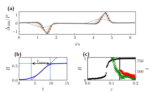
Figure 1: The collective PRC $\Delta_{100}$ for the Rayleigh model in Eq. (7) with perturbation strength $P$ is shown in (a). The black dots mark the PRC of the single oscillator and the lines the numerically measured values for $\varepsilon\in\{0.134,0.336,0.538,0.74,0.942\}$, where the collective PRC approaches the single oscillator PRC with increasing $\varepsilon$. In (b) the method for the calculation of the synchronization time $t_{sync}$ is visualized. The timescales for the synchronization and the relaxation are shown in (c). The black dots denote the magnitude of the limit cycle at the crossing of the positive $\dot{x}$-axis, the green crosses $t_{sync}$ and the red triangles $t_{relax}$. The necessary $\varepsilon$ for a stable limit cycle is marked with a black line.

The oscillators are perturbed simultaneously in the $\dot{x}$-direction with a small enough strength $P$, such that the collective PRC scales linearly with $P$ and Eq. (3) is valid. The resulting response of the mean-field is shown in Fig. 1(a). While the collective PRC is flat for small $\varepsilon$, it approaches the PRC of a single oscillator with increasing coupling strength. The approach to the PRC of a single oscillator is the expected outcome, as in the case of $\varepsilon\to\infty$, the oscillators will be fully synchronized and behave like a single unit.

An important property of the collective PRC is the needed relaxation time $t_{relax}$, as the application to real-world noisy systems becomes impossible if it is too long. When the oscillators are perturbed strongly before they fully relax, then the mean-field will not reach its limit cycle, and the phase dynamics in Eq. (3) are not applicable. To have a comparable timescale consider the synchronization time $t_{sync}$ in Fig. 1(b). It is measured as a linear approximation of the time needed to reach the stable distribution of oscillators, given by $R=\left|\boldsymbol{Z}\right|\approx const$, from a splay state, where all oscillators are distributed uniformly in the phase. The slope for the linear approximation is chosen as the value at the inflection point, i.e., the biggest $\dot{R}$. A comparison of the time scales in Fig. 1(c) shows that $t_{relax}$ (at about $40T$) is longer than $t_{sync}$. This suggests a very weak attraction to the stable distribution. The collective PRC can thus be only applied in an approximate sense.

3 Phase Dynamics of Coupled Oscillators

After investigating the phase dynamics under the influence of a perturbation, the next step of abstraction is the application of phase dynamics to coupled oscillators. Instead of the mean-field, the interest lies now on the single oscillatory units and their phases. The dynamics of coupled oscillators with coupling function $\boldsymbol{G}_{k}$ for oscillator $k$ and coupling strength $\varepsilon$ are

$$\frac{d\boldsymbol{y}_{k}}{dt}=\boldsymbol{f}_{k}(\boldsymbol{y}_{k})+\varepsilon\boldsymbol{G}_{k}(\boldsymbol{y}_{1},\boldsymbol{y}_{2},\ldots)\;.$$ (8)

The phase dynamics for such a system are given analogous to Eq. (2) with ${\varphi_{k}=\Phi_{k}(\boldsymbol{y}_{k})}$ as

$$\dot{\varphi}_{k}=\omega_{k}+\varepsilon\frac{\partial\Phi_{k}}{\partial\boldsymbol{y}_{k}}\boldsymbol{G}_{k}(\boldsymbol{y}_{1},\boldsymbol{y}_{2},\ldots)\;.$$ (9)

In this case, the phase does not grow uniformly. While it could be found on the limit cycle by virtue of the period, now the phases of all points in the state space have to be known to solve the coupling term. With the approximation of weak coupling, the dynamics stay close to the limit cycle of the uncoupled unit and the phases in this region are known, so the coupling function can be written in terms of these phases

$$\dot{\varphi}_{k}=\omega_{k}+\varepsilon G_{k}(\varphi_{k},\varphi_{1},\varphi_{2},\ldots)+\mathcal{O}(\varepsilon^{2})\;.$$ (10)

Higher-order approximations have to be considered to extend the phase dynamics farther past the limit cycle, for example, when considering higher coupling strengths.

Some methods for analytical phase reduction of higher-order consider systems with a separation of timescales kurebayashi2013phase ; pyragas2015phase or use isostable coordinates wilson2016isostable . A general method that only works for systems with a known phase in the autonomous systems uses a perturbation Ansatz on the isochrones leon2019phase . To reconstruct the phase dynamics numerically, one typically uses a Fourier series to represent the coupling function and then fits the coefficients using, e.g., a multiple shot tokuda2007inferring or Bayesian methods stankovski2016alterations . Other numerical reductions include reconstruction of the phase from a polar phase that is determined by a Hilbert transformation kralemann2008phase ; kralemann2011reconstructing or directly with an iterative Hilbert transform gengel2019phase . Some improvements can be made by using absolute phases in the coupling function instead of phase differences blaha2011reconstruction or considering triplets of oscillators to find structural connectivity kralemann2014reconstructing .

3.1 Weakly Coupled Oscillators - Kuramoto Model

The Kuramoto model acebron2005kuramoto ; pikovsky2015dynamics describes a weakly pairwise all-to-all coupled system of oscillators. The first order approximation in Eq. (10) is valid and the dynamics can be written as

$$\dot{\varphi}_{k}=\omega_{k}+\frac{\varepsilon}{N}\sum_{j=1}^{N}\sin(\varphi_{j}-\varphi_{k}+\alpha_{k})\;.$$ (11)

The $\omega_{k}$ are the natural frequencies and the $\alpha_{k}$ the phase shift parameters.

By using the complex mean-field $Z=Re^{i\theta}=1/N\sum_{j}e^{i\varphi_{j}}$ the system can be reduced to

$$\dot{\varphi}_{k}=\omega_{k}+\varepsilon R\sin(\theta-\varphi_{k}+\alpha_{k})\;.$$ (12)

The order parameter $R$ describes the degree of synchronization, $R=1$ denotes full synchrony and $R=0$ is an indicator for incoherence or antisymmetry.

One of the most important properties of this model is the analytical solvability. In the case of identical oscillators, the powerful Watanabe-Strogatz (WS) theory can be used watanabe1993integrability ; watanabe1994constants . It allows for the reduction of the dynamics from $N$ dimensions to just $3$ and $N-3$ constants of motion. The remaining degrees of freedom are three variables $\rho$, $\Psi$ and $\Theta$. Between them and the mean-field exists a correspondence, although they are not equal. Generally, $\rho$ and $\Theta$ are close to $R$ and $\theta$, while the final variable $\Psi$ can be seen as a measure of the system’s clustering. The correspondence between the degrees of freedom and the mean-field becomes even bigger in the thermodynamic limit when the dynamics move on the Ott-Antonsen manifold ott2008low ; ott2009long and reduced to just the mean-field variables, $R$ and $\theta$. The Ott-Antonsen manifold can only be seen as an asymptotic solution, as the transients can be very long pikovsky2011dynamics ; mirollo2012asymptotic .

When investigating multiple ($M$) groups of oscillators, the Kuramoto model can be extended to the M-Kuramoto model. The groups interact with different coupling strength and may have phase shifts,

$$\dot{\varphi}_{k}^{\sigma}=\omega_{k}^{\sigma}+\sum_{\sigma^{\prime}=1}^{M}\frac{\varepsilon_{\sigma,\sigma^{\prime}}}{N}\sum_{j=1}^{N_{\sigma^{\prime}}}\sin(\varphi_{j}^{\sigma^{\prime}}-\varphi_{k}^{\sigma}+\alpha_{\sigma,\sigma^{\prime}})\;.$$ (13)

Here $\sigma$ and $\sigma^{\prime}$ denote the different groups and $\varepsilon_{\sigma,\sigma^{\prime}}$ and $\alpha_{\sigma,\sigma^{\prime}}$ are the coupling strengths and phase shifts between groups $\sigma$ and $\sigma^{\prime}$, respectively.

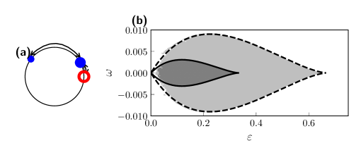
Figure 2: The solitary state in an M-Kuramoto model is visualized in (a). The red ring shows the attractive cluster, the big blue circle the repulsive cluster and the small blue circle the solitary oscillator. In (b) the existence of the solitary state is plotted. The dashed black line shows the analytical prediction for $N_{a}=N_{r}=5$ and the light gray area the numerical observation. The solid black line and dark gray area show the same, but for $N_{a}=N_{r}=8$.

Consider the system with ${\varepsilon_{\sigma,\sigma^{\prime}}=\varepsilon_{\sigma^{\prime}}}$ and ${\alpha_{\sigma,\sigma^{\prime}}=\alpha_{\sigma^{\prime}}}$ and two groups of identical oscillators, one attractive $\varphi^{a}$ and one repulsive $\varphi^{r}$

$$\dot{\varphi}_{k}^{a} =\omega_{a}+\frac{1}{N}\sum_{j=1}^{N_{a}}\sin(\varphi_{j}^{a}-\varphi_{k}^{a}+\alpha_{a})-\frac{1+\varepsilon}{N}\sum_{j=1}^{N_{r}}\sin(\varphi_{j}^{r}-\varphi_{k}^{a}+\alpha_{r})$$ (14)

$$\dot{\varphi}_{k}^{r} =\omega_{r}+\frac{1}{N}\sum_{j=1}^{N_{a}}\sin(\varphi_{j}^{a}-\varphi_{k}^{r}+\alpha_{a})-\frac{1+\varepsilon}{N}\sum_{j=1}^{N_{r}}\sin(\varphi_{j}^{r}-\varphi_{k}^{r}+\alpha_{r})\;,$$

where the time was rescaled such that the attractive group has coupling strength $1$ and the repulsive ${-(1+\varepsilon)}$. Then $\varepsilon$ no longer measures the coupling strength, but the excess of repulsive coupling. These equations can be reduced further by introducing the mean-fields of the groups ${Z_{a,r}=1/N_{a,r}\sum e^{i\varphi_{a,r}}}$, as before, and a common forcing

$$H=\frac{N_{a}}{N}e^{i\alpha_{a}}Z_{a}-\frac{N_{r}}{N}(1+\varepsilon)e^{i\alpha_{r}}Z_{r}\;.$$ (15)

The reduced equations are

$$\dot{\varphi}_{a} =\omega_{a}+{\rm Im}\left[He^{-i\varphi_{a}}\right]$$ (16)

$$\dot{\varphi}_{r} =\omega_{r}+{\rm Im}\left[He^{-i\varphi_{r}}\right]$$

and allow for the application of the WS theory to the system pikovsky2008partially .

In the system without natural frequencies ${\omega_{k}^{\sigma}=0}$ there exists a peculiar solitary state maistrenko2014solitary , see Fig. 2(a). When both groups have the same size ${N_{a}=N_{r}}$, the attractive group, and all the repulsive oscillators, except for one, will cluster at the same point. The remaining repulsive oscillator will be phase-shifted by $\pi$. In the case of ${\alpha_{\sigma^{\prime}}=0}$, the state exists for all values of $N$ in some region of $\varepsilon$ (which shrinks for increasing $N$), but it does not have full measure, i.e., some initial conditions may lead to a different state. For ${\alpha_{\sigma^{\prime}}\neq 0}$, the state only exists up to a critical system size and without full measure. The state’s existence is also predicted by the WS theory and is the only allowed clustered state, except for full synchrony.

Since the solitary state is a rather new discovery, there are slightly different definitions of it. The most popular one is that in a system with a natural order of the oscillators, e.g., ordered by their natural frequency, some single oscillators behave differently than the rest of the population and, more importantly, than their immediate neighbors. This is the main difference to a chimera state, where a whole subpopulation exhibits a different behavior. Kapitaniak et al. observed such a state in Ref. kapitaniak2014imperfect with metronomes coupled in a ring to their nearest neighbor and second nearest neighbor. In such a configuration, some single oscillators’ phases will differ from the rest of their synchronized neighbors. Another observation was made in Ref. hizanidis2016chimera , where superconducting quantum interference devices were placed in a one-dimensional array and coupled magnetically. In this case, the solitary oscillators exhibit a higher amplitude than the rest of the population.

The solitary state has also been found numerically in simulations of coupled Lorenz oscillators shepelev2018chimera and in a ring of coupled Stuart-Landau oscillators with symmetry breaking attractive and repulsive long-range coupling sathiyadevi2019long . The observation of the existence in multiplex networks of FitzHugh-Nagumo oscillators coupled in rings with a small mismatch in the intra-layer couplings mikhaylenko2019weak , allows even for controlling strategies to tune the dynamics in, e.g., neural networks.

While the existence has been shown in many different systems, there are only a few results in investigating its emergence and stability. In a Kuramoto model with inertia, the solitary state arises from a homoclinic bifurcation and persists even in the thermodynamic limit jaros2018solitary , in contrast to it being a finite size effect in the M-Kuramoto model with attractive and repulsive interaction. Aside from differential equations, the solitary state has also been found in coupled maps. Multiplex network of non-locally coupled maps with a singular hyperbolic attractor exhibit solitary states in their transition from coherence to incoherence rybalova2017transition ; semenova2017coherenceincoherence . During the transition, more and more solitary oscillators appear, growing almost linearly with the decrease in the coupling strength. This is the result of an increase of the size of the basin of attraction of the solitary set with a decrease in the coupling, as more random initial conditions lie in this basin semenova2018mechanism . To also induce solitary states in maps with nonhyperbolic attractors, a multiplicative noise can be added to the coupling constant, thus also showing the existence of the solitary state in a noisy system rybalova2018mechanism .

These solitary state can consist of multiple solitary oscillators, but from here on, a solitary state is defined more narrowly, such that a single oscillator shows a different behavior than the rest of the population.

In Ref. teichmann2019solitary we extend the M-Kuramoto model from Ref. maistrenko2014solitary to consider non-identical groups without phase shift ${\alpha_{a}=\alpha_{r}=0}$. The oscillators in each group are identical, but there exists a difference in the natural frequencies $\omega$, i.e., in Eqs. (14) ${\omega_{a}=0}$ and ${\omega_{r}=\omega}$. In this case the solitary state changes: the cluster of the repulsive oscillator has a small phase-shift in relation to the cluster of the attractive oscillators and the phase-shift between the repulsive cluster (or the attractive cluster) and the solitary oscillator is no longer $\pi$. The solitary state also has full measure, it will always be reached, regardless of the initial condition. The region of existence of the solitary state, as well as the phase shifts between the clusters and the solitary oscillator can be calculated and fits well to numerical observations, see Fig. 2(b). The state is also not stationary, but rotates with a constant frequency

$$\nu=\frac{1+\varepsilon}{\varepsilon}\omega\;.$$ (17)

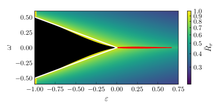
Figure 3: Parameter space of the M-Kuramoto model in Eqs. (14) with non-identical groups. The color shows the average order parameter of the repulsive group $\bar{R}_{r}$. Full synchrony is denoted by the black region, the solitary state by the red region and the white lines show the condition of existence for the fully synchronous state.

Aside from the solitary, there exist two other states in the system (Fig. 3), a fully synchronous state and a self-consistent partial synchronous state. In the fully synchronous state both clusters are fully synchronized, have a constant phase shift, and rotate with a uniform frequency. The region of existence and the stability of the state can be calculated directly from Eqs. (14). The results show that the region of stability with

$$\omega=\pm\sqrt{-\frac{\varepsilon^{3}}{2}-\frac{\varepsilon^{4}}{4}}$$ (18)

is slightly smaller than the region of existence, which fits the numerical results in Fig. 3. The frequency has the same relation as the solitary state in Eq. (17). We also find numerically that the attractive group always fully synchronizes, even outside the fully synchronous state, although there is no analytical proof for this. A simple check of the stability for the attractive cluster yields the inequality

$$R_{r}\cos(\theta_{r}-\theta_{a})<(1+\varepsilon)^{-1}\;.$$ (19)

The exact dynamics of the mean-field quantities are unknown, so this cannot be solved analytically, but simulations show that ${\theta_{r}-\theta_{a}}$ is quite small and $R_{r}$ falls off very quickly with $\varepsilon$ so that this equality is always fulfilled, and the attractive group fully synchronizes.

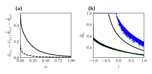
Figure 4: Goodness of fit for the WS theory in the M-Kuramoto model from Eqs. (14). In (a) the difference between the numerical ($\bar{\nu}_{n,r}$) and analytical ($\bar{\nu}_{a,r}$) average frequency for the single oscillators (dashed black line) and the mean-field (solid black line, $\bar{\dot{\theta}}_{r}$) of the repulsive group is shown. The frequencies were averaged over 100 different initial conditions for $N_{a}=N_{r}=5$ and $\varepsilon=0.5$. In (b) the average order parameter is plotted, where the blue crosses (black dots) show different initial conditions for $\omega=0.02$ ($\omega=0.6$) and their analytical value as a solid black line (green dashed line).

The final state, self-consistent partial synchrony, is defined by the difference in average frequencies between the single oscillators and their mean-field clusella2016minimal . The oscillators of the repulsive group move at a frequency that is generally faster than their mean-field. The WS theory cannot be applied to the whole system at once to explain this behavior, but on each group separately pikovsky2008partially . Making the crude approximation of the thermodynamic limit as well as stationarity (numerically we find that the average frequencies of both mean-fields coincide), allows for the calculation of the mean-field variables on the Ott-Antonsen manifold. As expected, they do not fit well for small $\omega$ or $\varepsilon$, but give a surprisingly good approximation for big $\omega$ and $\varepsilon$, even for a small system of ${N_{a}=N_{r}=5}$, see Fig. 4. With the now known average values of $R_{r}$ and $\dot{\theta}_{r}$ it is possible to calculate the average frequency of the oscillators in the WS theory baibolatov2009periodically as (bars denote the time-average)

$$\bar{\nu}_{r}=\frac{1-\bar{R}_{r}^{2}}{1+\bar{R}_{r}^{2}}\omega+\frac{2\bar{R}_{r}^{2}}{1+\bar{R}_{r}^{2}}\bar{\dot{\theta}}_{r}\;,$$ (20)

which shows clearly the expected difference between the average frequency of the mean-field and the single oscillators.

Even in a simple model of phase coupled oscillators in the weak coupling limit, it is possible to find interesting dynamical states. This can be extended further by considering more complex coupling schemes than simple all-to-all coupling. For even richer dynamics, higher-order coupling terms need to be considered.

3.2 Higher Order Phase Dynamics - Stuart-Landau Model

Extending the first order phase approximation for coupled oscillators in Eq. (10) to higher orders needs knowledge of the phase dynamics of the uncoupled units. One of the oscillators with a known analytical phase is the Stuart-Landau oscillator pikovsky2003synchronization ; landau1944problem . Its dimensionless dynamics in a coupled system are

$$\frac{dA}{dt}=(1+i\omega)A-\left|A\right|^{2}A-i\gamma A(\left|A\right|^{2}-1)+\varepsilon G(A_{1},A_{2},\ldots)\;,$$ (21)

where $A$ is a complex amplitude, $\omega$ is the frequency and $\gamma$ is the non-isochronicity parameter and determines $\Phi(A)$. Using ${A=Re^{i\theta}}$ leads to

$$\dot{R} =R-R^{3}+\varepsilon{\rm Re}\left[e^{-i\theta}G\right]$$ (22)

$$\dot{\theta} =\omega-\gamma(R^{2}-1)+\varepsilon R^{-1}{\rm Im}\left[e^{-i\theta}G\right]\;.$$

From there it follows for the phase of the uncoupled system ${\varphi=\theta-\gamma\ln(R)}$ and

$$\dot{R} =R-R^{3}+\varepsilon{\rm Re}\left[e^{-i(\varphi+\gamma\ln R)}G\right]$$ (23)

$$\dot{\varphi} =\omega+\varepsilon R^{-1}\left({\rm Im}\left[e^{-i(\varphi+\gamma\ln R)}G\right]-\gamma{\rm Re}\left[e^{-i(\varphi+\gamma\ln R)}G\right]\right)\;.$$

In Ref. matheny2019exotic , eight nanomechanical systems (NEMS) with dynamical equations resembling the Stuart-Landau oscillator were coupled in a circle. The oscillators were connected with their two neighbors, and the coupling term consisted of the average of them. The resulting phase reduction up to the second order in the coupling strength contained terms not present as physical links in the coupling scheme, such as ${\sin(\varphi_{k+2}-\varphi_{k})}$, ${\sin(\varphi_{k+2}-2\varphi_{k+1}+\varphi_{k})}$ and similar terms in the opposite direction. These non-structural terms only appear in the second-order approximation and would not be recovered in the typical first-order phase reduction. The observed system exhibits many dynamical states, such as traveling waves or weak chimeras, which would not necessarily be expected in the first-order phase approximation. Numerical simulations of the phase model show good agreement with the experimental results, pointing to the importance of the non-structural coupling terms in complex synchronization behavior.

Similarly, in Ref. leon2019phase a system of coupled Stuart-Landau oscillators was investigated numerically. The oscillators were coupled all-to-all to their mean-field. In the phase reduction up to the second-order in $\varepsilon$ appeared terms of the form ${\sin(\varphi_{m}+\varphi_{n}-2\varphi_{k})}$, where $m$, $n$ and $k$ are all possible combinations, coupling three oscillators. They determined that these terms are necessary to explain the system’s full dynamics but are again not present in the first-order phase dynamics, which only contains the existing pairwise connections.

In both Refs leon2019phase ; matheny2019exotic with coupled Stuart-Landau-like oscillators, the first-order approximation of the phase dynamics yields a Kuramoto-like model. This allows the novel terms to be seen as an extension of the Kuramoto model in Eq. (11) to higher coupling strength.

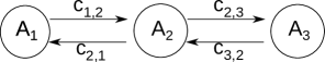
Figure 5: A system of three Stuart-Landau oscillators coupled in a line. The $A_{k}$ denote the complex amplitudes and the $c_{j,k}$ the coupling terms between the oscillators.

Based on the observations for the NEMS we investigated the higher order phase reduction for a system of three coupled nonidentical Stuart-Landau oscillators in Ref. gengel2020high . In difference to Ref. leon2019phase one pairwise connection is missing. The coupling scheme is a line, as can be seen in Fig. 5 and is given by

$$G_{k}(A_{k},A_{k-1},A_{k+1})=c_{k-1,k}e^{i\beta_{k-1,k}}A_{k-1}+c_{k+1,k}e^{i\beta_{k+1,k}}A_{k+1}\;,$$ (24)

where the $c_{j,k}$ are of ${\mathcal{O}(1)}$ and the $\beta_{j,k}$ are phase shifts between the two oscillators. To extend the phase reduction beyond the first order in $\varepsilon$ we use a perturbation method, where the $R$ and $\dot{\varphi}$ are functions of the phases and expand them as a power series

$$R =1+\varepsilon r^{(1)}(\varphi,\varphi_{1},\varphi_{2},\ldots)+\varepsilon^{2}r^{(2)}(\varphi,\varphi_{1},\varphi_{2},\ldots)+\ldots$$ (25)

$$\dot{\varphi} =\omega+\varepsilon\psi^{(1)}(\varphi,\varphi_{1},\varphi_{2},\ldots)+\varepsilon^{2}\psi^{(2)}(\varphi,\varphi_{1},\varphi_{2},\ldots)+\ldots\;.$$

In the dimensionless form the limit cycle of the uncoupled oscillator has the amplitude ${R_{0}=1}$, as can be easily checked in Eq. (22). Inserting these assumptions in Eqs. (23), the dynamics of $r^{(1)}$, $r^{(2)}$, $\psi^{(1)}$, $\psi^{(2)}$ and so on can be found by gathering the powers of $\varepsilon$. The full calculation is rather long, so please see Ref. gengel2020high for a detailed explanation. Here it will suffice to say that to find the phase dynamics in the second order in $\varepsilon$, a partial differential equation has to be solved using a Fourier series to represent the coupling function $G_{k}$. This representation is motivated by the fact that $G_{k}$ has to be $2\pi$-periodic for all the phases. The resulting reduction for the first oscillator up to the second order in $\varepsilon$ is

$$\dot{\varphi}_{1} =\omega_{1}+\varepsilon c_{2,1}[\sin(\varphi_{2}-\varphi_{1}+\beta_{2,1})-\gamma\cos(\varphi_{2}-\varphi_{1}+\beta_{2,1})]$$ (26)

$$+\varepsilon^{2}\left[a_{1;0,0,0}^{(2)}+a_{1;-2,2,0}^{(2)}\cos(2\varphi_{2}-2\varphi_{1})+b_{1;-2,2,0}^{(2)}\sin(2\varphi_{2}-2\varphi_{1})\right.$$

$$\left.+a_{1;-1,2,-1}^{(2)}\cos(2\varphi_{2}-\varphi_{1}-\varphi_{3})+b_{1;-1,2,-1}^{(2)}\sin(2\varphi_{2}-\varphi_{1}-\varphi_{3})\right.$$

$$\left.+a_{1;-1,0,1}^{(2)}\cos(\varphi_{3}-\varphi_{1})+b_{1;-1,0,1}^{(2)}\sin(\varphi_{3}-\varphi_{1})\right]\;,$$

with $a_{k;\boldsymbol{l}}^{(j)}$ and $b_{k;\boldsymbol{l}}^{(j)}$ denoting the coefficients for cosine and sine terms respectively and $k$ being the index of the oscillator. A vector of integers $\boldsymbol{l}$ contains the coefficients before the phases and $j$ the power in $\varepsilon$.

Using the perturbation method up to the second order in $\varepsilon$ yields again non-structural terms in Eq. (26), e.g. terms of the form ${\sin(\varphi_{3}-\varphi_{1})}$. Aside from these, there exist additional terms coupling all three oscillators ${\sin(2\varphi_{2}-\varphi_{1}-\varphi_{3})}$ and second harmonics ${\sin(2\varphi_{2}-2\varphi_{1})}$. The coefficients of the second order also contain the frequency difference between the oscillators, whereas the first order terms do not.

A Fourier Ansatz is used to measure the coupling terms numerically and verify the analytical results. The phase dynamics are ${2\pi}$-periodic, so they can be written as a multidimensional Fourier series

$$\dot{\varphi}_{k}=a_{k;\boldsymbol{0}}+\sum_{\boldsymbol{l}\neq 0}\left[a_{k;\boldsymbol{l}}\cos(\boldsymbol{\varphi}\cdot\boldsymbol{l})+b_{k;\boldsymbol{l}}\sin(\boldsymbol{\varphi}\cdot\boldsymbol{l})\right]\;,$$ (27)

where ${\boldsymbol{\varphi}=(\varphi_{1},\varphi_{2},\ldots,\varphi_{N})}$ is a vector of all the phases, $\boldsymbol{l}$ an N-dimensional vector of integers and ${\boldsymbol{\varphi}\cdot\boldsymbol{l}=\sum_{j}\varphi_{j}l_{j}}$ the scalar product. The $a_{k,\boldsymbol{l}}$ and $b_{k,\boldsymbol{l}}$ are Fourier coefficients. This form resembles the analytical results in Eq. (26) and finding the relevant coupling terms is reduced to fitting the Fourier coefficients $a_{k;\boldsymbol{l}}$ and $b_{k;\boldsymbol{l}}$ up to some maximum value with ${\left|l_{j}\right|\leq m}$. Because the coupling function is real, ${a_{k;-\boldsymbol{l}}=-a_{k;\boldsymbol{l}}}$ and the number of coefficients to consider halves. Still, the number of terms that need to be fitted scales like $m^{3}$, which increases the necessary number of data points for a good fit very rapidly with $m$ and leads to the curse of dimensionality.

In the case of partial synchrony, the Fourier coefficients can be fitted onto one long time series, although some initial transient has to be integrated over before the dynamics reach the torus spanned by the phases. For a good fit, the trajectory should be long enough to cover the whole torus. However, this is not the case in the synchronous regime; instead, the dynamics will settle on a single synchronized trajectory. The integration has to be stopped before reaching this synchronous trajectory and restarted with different initial conditions until the torus is sufficiently filled.

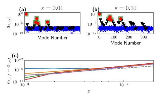
Figure 6: Comparison of analytical and numerically fitted modes for the Stuart-Landau oscillators with coupling function Eq. (24) in the partial synchronous regime. The modes shown are the cosine terms for the first oscillator in Eq. (26). In (a) and (b) the red circles denote numerically fitted values for terms appearing in Eq. (26), while their analytical values are shown as green boxes. Black triangles denote terms ${\sum_{j}l_{j}=0}$, which are the only allowed terms, because of rotational symmetry. The blue crosses are all other modes up to ${\boldsymbol{l}=(4,4,4)}$. In (c) the difference between the analytical and numerically fitted modes are shown. The gray dashed line is a polynomial $\varepsilon^{3}$, so the error scales stronger than $\varepsilon^{3}$.

Fitting the coefficients for different coupling strengths $\varepsilon$ yields the power series

$$a_{k;\boldsymbol{l}}=a_{k;\boldsymbol{l}}^{(0)}+\varepsilon a_{k;\boldsymbol{l}}^{(1)}+\varepsilon^{2}a_{k;\boldsymbol{l}}^{(2)}+\ldots$$ (28)

and a similar series for $b_{k;\boldsymbol{l}}$. The coupling function is then reconstructed by comparing these series and Eq. (27). The results of this method fit very well to the analytical prediction, as can be seen in Fig. 6.

The numerical method to reconstruct the phase can also be used in cases where the phase is unknown, but then the phases and their derivatives have to be calculated numerically. For finding the phase, an autonomous copy of each oscillator is integrated. It evolves for a number of its autonomous periods $T$ until it reaches its limit cycle. The phase after the relaxation is then also the phase of the point before the relaxation. To find the derivative, one observes the infinitesimal time step $dt$ of the perturbed system and sets it in relation to a different time step $\overline{dt}$ on the limit cycle. This time difference $\overline{dt}$ is determined by the motion on the limit cycle and the derivative $\boldsymbol{f}$ in Eq. (1). Using the relation of $dt$ and $\overline{dt}$ allows the calculation of the phase derivative, even if the oscillator is perturbed far from its limit cycle. For a full explanation and the resulting equation, see Ref. gengel2020high .

4 Summary

Phase dynamics are an important tool to analyze dynamical systems. In the case of a simple perturbation of an ensemble of oscillators, this reduces, in the first order, to the collective PRC. The PRC has been investigated for a system of coupled Rayleigh oscillators, where it took a long time to fully relax back onto the limit cycle after the perturbation, even in comparison to the time needed for synchronization. This makes the collective PRC only usable as an approximate description in noisy environments, where it is perturbed again before it can fully settle.

In the paradigmatical Kuramoto model with two groups, one attractive and one repulsive, an interesting solitary state is observed that does not appear in a model with just one group. A single solitary oscillator leaves its otherwise fully synchronized group in this state and gets phase-shifted by $\pi$. The use of groups with different natural frequencies leads to a stabilization of this state.

In the case of phase dynamics for the description of a coupled system, most of the current works use the first-order phase approximation. The first-order reduction for pairwise coupled units yields only pairwise terms in the phase model. When extending the phase reduction beyond the first-order, new connections arise that are necessary to describe more complicated dynamics. Even in a simple model of three Stuart-Landau oscillators, coupled in a line, the second-order approximation consists only of higher-order or non-structural terms. The analytical derivation of the additional terms follows from a simple perturbation Ansatz. A numerical verification shows good agreement and supports the analytical findings.

- (1) E. Kaempfer, The history of Japan: together with a description of the kingdom of Siam, 1690-92, vol. 3. AMS Press, 1906.
- (2) A. Pikovsky, M. Rosenblum, and J. Kurths, Synchronization: a universal concept in nonlinear sciences, vol. 12. Cambridge university press, 2003.
- (3) Y. Kuramoto and D. Battogtokh, “Coexistence of coherence and incoherence in nonlocally coupled phase oscillators.,” Nonlinear Phenomena in Complex Systems, vol. 5, no. 4, pp. 380–385, 2002.
- (4) T. Qiu, S. Boccaletti, I. Bonamassa, Y. Zou, J. Zhou, Z. Liu, and S. Guan, “Synchronization and bellerophon states in conformist and contrarian oscillators,” Scientific reports, vol. 6, 2016.
- (5) A. Hooper and R. Grimshaw, “Travelling wave solutions of the Kuramoto-Sivashinsky equation,” Wave Motion, vol. 10, pp. 405–420, oct 1988.
- (6) Y. Maistrenko, B. Penkovsky, and M. Rosenblum, “Solitary state at the edge of synchrony in ensembles with attractive and repulsive interactions,” Phys. Rev. E, vol. 89, p. 060901, Jun 2014.
- (7) S. H. Strogatz, D. M. Abrams, A. McRobie, B. Eckhardt, and E. Ott, “Theoretical mechanics: Crowd synchrony on the Millennium Bridge,” Nature, vol. 438, no. 7064, pp. 43–44, 2005.
- (8) B. van der Pol and J. van der Mark, “The heartbeat considered as a relaxation oscillation, and an electrical model of the heart,” The London, Edinburgh, and Dublin Philosophical Magazine and Journal of Science, vol. 6, no. 38, pp. 763–775, 1928.
- (9) I. Ashraf, R. Godoy-Diana, J. Halloy, B. Collignon, and B. Thiria, “Synchronization and collective swimming patterns in fish ( hemigrammus bleheri ),” Journal of The Royal Society Interface, vol. 13, p. 20160734, oct 2016.
- (10) M. Breakspear, S. Heitmann, and A. Daffertshofer, “Generative models of cortical oscillations: Neurobiological implications of the Kuramoto model,” Frontiers in Human Neuroscience, vol. 4, p. 190, 2010.
- (11) D. Cumin and C. Unsworth, “Generalising the kuramoto model for the study of neuronal synchronisation in the brain,” Physica D: Nonlinear Phenomena, vol. 226, no. 2, pp. 181–196, 2007.
- (12) T. Tateno and H. Robinson, “Phase resetting curves and oscillatory stability in interneurons of rat somatosensory cortex,” Biophysical Journal, vol. 92, no. 2, pp. 683 – 695, 2007.
- (13) W. Kurebayashi, S. Shirasaka, and H. Nakao, “Phase reduction method for strongly perturbed limit cycle oscillators,” Physical Review Letters, vol. 111, nov 2013.
- (14) I. León and D. Pazó, “Phase reduction beyond the first order: The case of the mean-field complex ginzburg-landau equation,” Physical Review E, vol. 100, jul 2019.
- (15) M. H. Matheny, J. Emenheiser, W. Fon, A. Chapman, A. Salova, M. Rohden, J. Li, M. H. de Badyn, M. Pósfai, L. Duenas-Osorio, M. Mesbahi, J. P. Crutchfield, M. C. Cross, R. M. D’Souza, and M. L. Roukes, “Exotic states in a simple network of nanoelectromechanical oscillators,” Science, vol. 363, p. eaav7932, mar 2019.
- (16) Y. Kuramoto, Chemical oscillations, turbulence and waves. Springer, Berlin, 1984.
- (17) E. Teichmann and M. Rosenblum, “Solitary states and partial synchrony in oscillatory ensembles with attractive and repulsive interactions,” Chaos: An Interdisciplinary Journal of Nonlinear Science, vol. 29, p. 093124, sep 2019.
- (18) E. Gengel, E. Teichmann, M. Rosenblum, and A. S. Pikovsky, “High-order phase reduction for coupled oscillators,” Journal of Physics: Complexity, oct 2020.
- (19) A. Winfree, The geometry of biological time. Berlin New York: Springer-Verlag, 1980.
- (20) S. Achuthan and C. C. Canavier, “Phase-resetting curves determine synchronization, phase locking, and clustering in networks of neural oscillators,” Journal of Neuroscience, vol. 29, no. 16, pp. 5218–5233, 2009.
- (21) J. L. P. Velazquez, R. G. Erra, and M. Rosenblum, “The epileptic thalamocortical network is a macroscopic self-sustained oscillator: Evidence from frequency-locking experiments in rat brains,” Scientific Reports, vol. 5, feb 2015.
- (22) D. Wilson and J. Moehlis, “Determining individual phase response curves from aggregate population data,” Physical Review E, vol. 92, aug 2015.
- (23) Z. Levnajić and A. Pikovsky, “Phase resetting of collective rhythm in ensembles of oscillators,” Physical Review E, vol. 82, p. 056202, Nov. 2010.
- (24) K. M. Hannay, V. Booth, and D. B. Forger, “Collective phase response curves for heterogeneous coupled oscillators,” Phys. Rev. E, vol. 92, p. 022923, Aug 2015.
- (25) J. Rayleigh and R. Lindsay, The Theory of Sound. No. v. 1 in Dover Books on Physics Series, Dover, 1945.
- (26) K. Pyragas and V. Novičenko, “Phase reduction of a limit cycle oscillator perturbed by a strong amplitude-modulated high-frequency force,” Physical Review E, vol. 92, jul 2015.
- (27) D. Wilson and J. Moehlis, “Isostable reduction of periodic orbits,” Physical Review E, vol. 94, nov 2016.
- (28) I. T. Tokuda, S. Jain, I. Z. Kiss, and J. L. Hudson, “Inferring phase equations from multivariate time series,” Physical Review Letters, vol. 99, aug 2007.
- (29) T. Stankovski, S. Petkoski, J. Raeder, A. F. Smith, P. V. E. McClintock, and A. Stefanovska, “Alterations in the coupling functions between cortical and cardio-respiratory oscillations due to anaesthesia with propofol and sevoflurane,” Philosophical Transactions of the Royal Society A: Mathematical, Physical and Engineering Sciences, vol. 374, p. 20150186, may 2016.
- (30) B. Kralemann, L. Cimponeriu, M. Rosenblum, A. Pikovsky, and R. Mrowka, “Phase dynamics of coupled oscillators reconstructed from data,” Physical Review E, vol. 77, jun 2008.
- (31) B. Kralemann, A. Pikovsky, and M. Rosenblum, “Reconstructing phase dynamics of oscillator networks,” Chaos: An Interdisciplinary Journal of Nonlinear Science, vol. 21, no. 2, p. 025104, 2011.
- (32) E. Gengel and A. Pikovsky, “Phase demodulation with iterative hilbert transform embeddings,” Signal Processing, vol. 165, pp. 115–127, dec 2019.
- (33) K. A. Blaha, A. Pikovsky, M. Rosenblum, M. T. Clark, C. G. Rusin, and J. L. Hudson, “Reconstruction of two-dimensional phase dynamics from experiments on coupled oscillators,” Physical Review E, vol. 84, oct 2011.
- (34) B. Kralemann, A. Pikovsky, and M. Rosenblum, “Reconstructing effective phase connectivity of oscillator networks from observations,” New Journal of Physics, vol. 16, p. 085013, aug 2014.
- (35) J. A. Acebrón, L. L. Bonilla, C. J. P. Vicente, F. Ritort, and R. Spigler, “The Kuramoto model: A simple paradigm for synchronization phenomena,” Reviews of modern physics, vol. 77, no. 1, p. 137, 2005.
- (36) A. Pikovsky and M. Rosenblum, “Dynamics of globally coupled oscillators: Progress and perspectives,” Chaos: An Interdisciplinary Journal of Nonlinear Science, vol. 25, no. 9, p. 097616, 2015.
- (37) S. Watanabe and S. H. Strogatz, “Integrability of a globally coupled oscillator array,” Phys. Rev. Lett., vol. 70, pp. 2391–2394, Apr 1993.
- (38) S. Watanabe and S. H. Strogatz, “Constants of motion for superconducting Josephson arrays,” Physica D: Nonlinear Phenomena, vol. 74, no. 3, pp. 197 – 253, 1994.
- (39) E. Ott and T. M. Antonsen, “Low dimensional behavior of large systems of globally coupled oscillators,” Chaos: An Interdisciplinary Journal of Nonlinear Science, vol. 18, p. 037113, Sept. 2008.
- (40) E. Ott and T. M. Antonsen, “Long time evolution of phase oscillator systems,” Chaos: An Interdisciplinary Journal of Nonlinear Science, vol. 19, no. 2, p. 023117, 2009.
- (41) A. Pikovsky and M. Rosenblum, “Dynamics of heterogeneous oscillator ensembles in terms of collective variables,” Physica D: Nonlinear Phenomena, vol. 240, no. 9, pp. 872–881, 2011.
- (42) R. E. Mirollo, “The asymptotic behavior of the order parameter for the infinite-n kuramoto model,” Chaos: An Interdisciplinary Journal of Nonlinear Science, vol. 22, no. 4, p. 043118, 2012.
- (43) A. Pikovsky and M. Rosenblum, “Partially integrable dynamics of hierarchical populations of coupled oscillators,” Phys. Rev. Lett., vol. 101, p. 264103, Dec 2008.
- (44) T. Kapitaniak, P. Kuzma, J. Wojewoda, K. Czolczynski, and Y. Maistrenko, “Imperfect chimera states for coupled pendula,” Scientific Reports, vol. 4, sep 2014.
- (45) J. Hizanidis, N. Lazarides, G. Neofotistos, and G. Tsironis, “Chimera states and synchronization in magnetically driven SQUID metamaterials,” The European Physical Journal Special Topics, vol. 225, pp. 1231–1243, sep 2016.
- (46) I. A. Shepelev, G. I. Strelkova, and V. S. Anishchenko, “Chimera states and intermittency in an ensemble of nonlocally coupled Lorenz systems,” Chaos: An Interdisciplinary Journal of Nonlinear Science, vol. 28, p. 063119, jun 2018.
- (47) K. Sathiyadevi, V. K. Chandrasekar, D. V. Senthilkumar, and M. Lakshmanan, “Long-range interaction induced collective dynamical behaviors,” Journal of Physics A: Mathematical and Theoretical, vol. 52, p. 184001, apr 2019.
- (48) M. Mikhaylenko, L. Ramlow, S. Jalan, and A. Zakharova, “Weak multiplexing in neural networks: Switching between chimera and solitary states,” Chaos: An Interdisciplinary Journal of Nonlinear Science, vol. 29, p. 023122, feb 2019.
- (49) P. Jaros, S. Brezetsky, R. Levchenko, D. Dudkowski, T. Kapitaniak, and Y. Maistrenko, “Solitary states for coupled oscillators with inertia,” Chaos: An Interdisciplinary Journal of Nonlinear Science, vol. 28, no. 1, p. 011103, 2018.
- (50) E. Rybalova, N. Semenova, G. Strelkova, and V. Anishchenko, “Transition from complete synchronization to spatio-temporal chaos in coupled chaotic systems with nonhyperbolic and hyperbolic attractors,” The European Physical Journal Special Topics, vol. 226, pp. 1857–1866, jun 2017.
- (51) N. I. Semenova, E. V. Rybalova, G. I. Strelkova, and V. S. Anishchenko, “’Coherence–incoherence’ transition in ensembles of nonlocally coupled chaotic oscillators with nonhyperbolic and hyperbolic attractors,” Regular and Chaotic Dynamics, vol. 22, pp. 148–162, mar 2017.
- (52) N. Semenova, T. Vadivasova, and V. Anishchenko, “Mechanism of solitary state appearance in an ensemble of nonlocally coupled Lozi maps,” The European Physical Journal Special Topics, vol. 227, pp. 1173–1183, nov 2018.
- (53) E. Rybalova, G. Strelkova, and V. Anishchenko, “Mechanism of realizing a solitary state chimera in a ring of nonlocally coupled chaotic maps,” Chaos, Solitons & Fractals, vol. 115, pp. 300–305, oct 2018.
- (54) P. Clusella, A. Politi, and M. Rosenblum, “A minimal model of self-consistent partial synchrony,” New Journal of Physics, vol. 18, no. 9, p. 093037, 2016.
- (55) Y. Baibolatov, M. Rosenblum, Z. Z. Zhanabaev, M. Kyzgarina, and A. Pikovsky, “Periodically forced ensemble of nonlinearly coupled oscillators: From partial to full synchrony,” Phys. Rev. E, vol. 80, p. 046211, Oct 2009.
- (56) L. D. Landau, “On the problem of turbulence,” in Dokl. Akad. Nauk USSR, vol. 44, p. 311, 1944.