Mixed platoon control of automated and human-driven vehicles at a signalized intersection: dynamical analysis and optimal control

Abstract

The emergence of Connected and Automated Vehicles (CAVs) promises better traffic mobility for future transportation systems. Existing research mostly focused on fully-autonomous scenarios, while the potential of CAV control at a mixed traffic intersection where human-driven vehicles (HDVs) also exist has been less explored. This paper proposes a notion of “$1+n$” mixed platoon, consisting of one leading CAV and $n$ following HDVs, and formulates a platoon-based optimal control framework for CAV control at a signalized intersection. Based on the linearized dynamics model of the “$1+n$” mixed platoon, fundamental properties including stability and controllability are under rigorous theoretical analysis. Then, a constrained optimal control framework is established, aiming at improving the global traffic efficiency and fuel consumption at the intersection via direct control of the CAV. A hierarchical event-triggered algorithm is also designed for practical implementation of the optimal control method between adjacent mixed platoons when approaching the intersection. Extensive numerical simulations at multiple traffic volumes and market penetration rates validate the greater benefits of the mixed platoon based method, compared with traditional trajectory optimization methods for one single CAV.

1 Introduction

As planned points of conflict in urban traffic networks, intersections play a critical role in traffic mobility optimization. Existing research has shown that the frequent stop-and-go and idling behavior of individual vehicles when approaching the intersection is the main cause of traffic congestion and casualties Lee & Park [2012], Rakha et al. [2001]. Accordingly, trajectory optimization for individual vehicles at the intersection has attracted significant attention. In particular, the emergence of Connected and Automated Vehicles (CAVs) has provided new opportunities for improving the traffic performance at intersections. Compared to traditional human-driven vehicles (HDVs), CAVs can acquire accurate information of surrounding traffic participants and traffic signal phase and timing (SPAT) through vehicle-to-vehicle and vehicle-to-infrastructure communication Contreras-Castillo et al. [2017], and their velocity trajectories in approaching intersections can be directly optimized in the pursuit of higher traffic efficiency and lower fuel consumption. Multiple methods have been applied to CAV control at signalized intersections, including model predictive control Asadi & Vahidi [2011], Yang et al. [2017], fuzzy logic Milanés et al. [2010], Onieva et al. [2015] and optimal control Li et al. [2015], Jiang et al. [2017]. Moreover, the potential of cooperative control of traffic signals and CAVs has also been recently discussed Xu et al. [2018a].

The aforementioned research mainly considered a fully-autonomous scenario—the market penetration rate (MPR) of CAVs is 100%. In practice, however, it might take decades for all the HDVs in current transportation systems to be transformed into CAVs. Instead, a more practical scenario in the near future is a mixed traffic system where CAVs and HDVs coexist Zheng et al. [2020]. Existing research on mixed traffic intersections mostly focused on the estimation of traffic states and optimization of traffic signals Priemer & Friedrich [2009], Salman et al. [2017], Zheng & Liu [2017], Feng et al. [2015]. For example, Priemer et al. utilized dynamic programming to estimate the queuing length in the mixed traffic environment and then optimized the traffic phase time based on the estimated results Priemer & Friedrich [2009]. Some other methods, including fuzzy logic Salman et al. [2017], expectation maximization Zheng & Liu [2017] and dynamic programming Feng et al. [2018], have also been exploited to achieve a similar goal. To improve the estimation accuracy, the celebrated results on microscopic car-following models have been recently employed to describe the behaviors of HDVs, including Gipps Model Gipps [1981], Optimal Velocity Model (OVM) Helbing & Tilch [1998] and Intelligent Driver Model (IDM) Treiber & Kesting [2013]; see, e.g., Du et al. [2017], Fang et al. [2020].

Despite these existing works, the topic of CAV control, i.e., trajectory optimization of CAVs, in mixed traffic intersections has not been fully discussed. To tackle this problem, several works regarded HDVs as disturbances in the control of CAVs Du et al. [2017], Ala et al. [2016], or focused on the task of collision avoidance based on the prediction of HDVs’ behaviors Jiang et al. [2017], Ma et al. [2017]. It is worth noting that most of these methods were limited to improving the performance of CAVs themselves in their optimization frameworks, instead of optimizing the global traffic flow consisting of both HDVs and CAVs at the intersection. Two notable exceptions are in Zhao et al. [2018], Liang et al. [2019], which attempted to improve the performance at the signalized intersection from the perspective of the so-called mixed platoon. They enumerated several possible formations consisting of HDVs and CAVs, and investigated their effectiveness through small-scale simulation experiments. However, a general and explicit definition of the mixed platoon has not been clarified, and fundamental properties of the mixed platoon at intersections have been less explored. Moreover, a specific optimal control framework for the mixed platoon at intersections with global consideration of improving the entire traffic performance is still lacking.

In fact, considering the interaction between adjacent vehicles on the same lane, it is easy to understand that velocity trajectories of CAVs could have a certain influence on those of surrounding vehicles, especially the vehicles following behind them. Accordingly, the driving strategies of CAVs could have a direct impact on the performance of the entire mixed traffic intersection; such impact might even be negative when inappropriate CAV strategies are adopted Ala et al. [2016]. By contrast, when taking the performance of entire mixed traffic into explicit consideration, the optimization of CAVs’ trajectories could bring further benefits to traffic mobility. Such idea of improving the global traffic performance via controlling CAVs has been recently proposed as Lagrangian Control of traffic flow Stern et al. [2018], which has been discussed in various traffic scenarios, including closed ring road Zheng et al. [2020], open straight road Wang et al. [2020a], traffic bottleneck Vinitsky et al. [2018], and non-signalized intersection Wu et al. [2017]. Regarding signalized intersections, the potential of this notion has not been well understood.

In this paper, we focus on the scenario of a signalized intersection where HDVs and CAVs coexist and aim at improving the performance of the entire mixed traffic intersection through direct control of CAVs. To address this problem, we propose a novel framework which separates the traffic flow into “$1+n$” microstructures consisting of one leading CAV and $n$ following HDVs. Such microstructure is particularly common in the near future when the MPR is relatively low, which is named as “$1+n$” mixed platoon. We discuss the possibility of letting the first CAV lead the motion of following $n$ HDVs in approaching intersections, and show how to enable the CAV to benefit the global traffic mobility in the proposed structure of mixed platoon. First, we present the dynamics model of “$1+n$” mixed platoon systems based on linearized car-following models and investigate its fundamental properties, including open-loop stability and controllability. Then, we establish the optimal control framework for the mixed platoon and design a hierarchical algorithm to improve the global traffic mobility performance at a signalized intersection. Specifically, our contributions are as follows:

1. The notion of the “$1+n$” mixed platoon is proposed for trajectory optimization of CAVs at signalized intersections in the mixed traffic environment. Rather than enumerating the mixed platoon formations Zhao et al. [2018], Liang et al. [2019], we provide an explicit definition of the mixed platoon. Based on the linearized dynamics model, we perform a rigorous theoretical analysis of its fundamental properties, including open-loop stability and controllability. Our theoretical results reveal that the “$1+n$” mixed platoon is always controllable under a very mild condition, regardless of the platoon size $n$.

2. An optimal control framework is established for the “$1+n$” mixed platoon at a constant traffic SPAT intersection scenario. Instead of being limited to optimizing the performance of the CAVs only Asadi & Vahidi [2011], Yang et al. [2017], Milanés et al. [2010], Onieva et al. [2015], Li et al. [2015], Jiang et al. [2017], Du et al. [2017], Fang et al. [2020], Ala et al. [2016], Ma et al. [2017], our optimal control formulation aims at improving the global performance of the entire mixed traffic intersection. Precisely, the velocity deviations and fuel consumption of all the vehicles in the mixed platoon are under explicit consideration. Moreover, unlike Zhao et al. [2018], Liang et al. [2019], we optimize the terminal velocity setting to maximize the traffic throughput.

3. Finally, a hierarchical algorithm is proposed to accomplish the optimal control framework of “$1+n$” mixed platoons, which can be applied in any MPR of mixed traffic environments. An event-triggered mechanism is designed to avoid potential collisions of adjacent mixed platoons. Large-scale traffic simulations are conducted at multiple traffic volumes and MPRs, and it is observed that the proposed mixed platoon based control method surpasses the traditional intersection control method for single CAV Asadi & Vahidi [2011], Yang et al. [2017] in both traffic efficiency and fuel consumption.

The rest of this paper is organized as follows. Section 2 introduces the problem of the system modeling for the proposed“$1+n$” mixed platoon. Section 3 presents the system dynamics analysis, optimal control framework and algorithm design. The simulation results are shown in Section LABEL:Section:SimulationResult, and Section LABEL:Section:Conclusion concludes this paper.

2 Problem Statement

In this section, we firstly introduce the scenario setup, then present the dynamical modeling of individual vehicles and the mixed platoon systems.

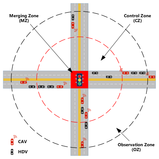
Figure 1: Illustration for the mixed traffic intersection. Red vehicles represent CAVs, which can transmit and receive vehicle information and the vehicle is fully autonomous driving. Black vehicles represent HDVs, which can only transmit ego vehicle information to other vehicles and are controlled by car following model.

2.1 Scenario Setup

In this paper, we consider a typical signalized intersection scenario in the mixed traffic environment, where HDVs and CAVs coexist; see Fig. 1 for illustration. A traffic light is deployed in the center to guide individual vehicles to drive through the intersection. Note that CAVs follow the instructions from a central cloud coordinator, which collects information from all the involved vehicles around the intersection and calculates the optimal velocity trajectories for each CAV. The design of the control strategies for the central cloud coordinator is presented in Section 3.

Motivated by previous works on signalized intersections Feng et al. [2015], Malikopoulos et al. [2018], Bian et al. [2019], we separate the intersection into three zones, as illustrated in Fig. 1. The red square area in the center is named as the Merging Zone (MZ), which is the area of potential lateral collision of the involved vehicles. The ring area between two dashed lines is called the Observation Zone (OZ), where the CAVs and HDVs are allowed to perform lane-changing behaviors. The area between OZ and MZ is the Control Zone (CZ), where the CAVs are under direct control from the central cloud coordinator. The specific range of each zone is discussed in Section LABEL:Section:SimulationResult.

Similar to existing research Zhao et al. [2018], Liang et al. [2019], the following assumptions are needed to facilitate the control design for signalized intersection controls, as well as the system modeling and dynamics analysis.

1. All the vehicles are connected vehicles, which means that both the CAVs and the HDVs are able to transmit their velocity and position to the central cloud coordinator through wireless communication, e.g., V2I communication Gerla et al. [2014]. An ideal communication condition without communication delay or packet loss is under consideration.

2. All the CAVs are capable of fully autonomous driving, which follow the velocity trajectories assigned from the central cloud coordinator after they enter CZ. Regarding the HDVs, they are controlled by human drivers, for which we assume a general car-following model to describe their driving behavior (see Section 2.2 for details).

3. Lane changing is not permitted in CZ. As shown in Ala et al. [2016], Xu et al. [2018b], unexpected lane changing behaviors might worsen the traffic efficiency, especially near the intersection. Therefore, lane changing is only allowed in OZ, while In CZ, we only need to focus on the longitudinal behavior of each vehicle.

2.2 Dynamical Modeling of Mixed Platoon Systems

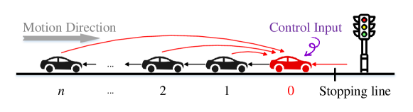
Figure 2: Schematic for the “$1+n$” mixed platoon. Red arrows denote the information flow of the leading CAV (colored in red), which collects information from the following HDVs as well as the traffic light and has an external control input. Black arrows represent the information flow of the HDVs (colored in black), which are under control by human drivers and only acquire information from the preceding vehicle, as shown in (1). Note that the coordinate origin is set at the stopping line, where the vehicle position is $x=0$.

In this paper, we propose the notion of “$1+n$” mixed platoon as shown in Fig. 2. It consists of one leading CAV and $n$ following HDVs. Specifically, each CAV is designed as the leading vehicle of the mixed platoon, which leads the motion of the following $n$ HDVs with the aim of improving the performance of the entire mixed platoon when passing the intersection.

Consider the $n$ following HDVs in the mixed platoon illustrated in Fig. 2. We denote the position and velocity of vehicle $i$ at time $t$ as $x_{i}(t)$ and $v_{i}(t)$, respectively. The headway distance of vehicle $i$ from vehicle $i-1$ is defined as ${d}_{i}(t):=x_{i-1}(t)-x_{i}(t)$. Then, $\dot{v}_{i}(t)$ and $\dot{d}_{i}(t)=v_{i-1}(t)-v_{i}(t)$ represents the acceleration of vehicle $i$, and the relative velocity of vehicle $i$ from vehicle $i-1$, respectively.

A great many efforts have been made in previous works to describe the HDVs’ car-following dynamics, with several significant models developed, e.g., OVM Helbing & Tilch [1998] and IDM Treiber & Kesting [2013]. As shown in the literature Zheng et al. [2020], Wilson & Ward [2011], most of them can be expressed as the following general form ($i=1,\ldots,n$)

$$\dot{v}_{i}(t)=F\left(d_{i}(t),\dot{d}_{i}(t),v_{i}(t)\right),$$ (1)

which means that the acceleration of vehicle $i$ is determined by its headway distance, relative velocity and its own velocity.

In this paper, we require that the mixed platoon passes the intersection at a pre-specified equilibrium velocity $v^{\ast}$. In equilibrium traffic state, we have $\dot{d}_{i}(t)=0$ for $i=1,\ldots,n$, and thus each vehicle has a corresponding equilibrium headway distance $d^{\ast}$, where it holds that

$$F\left(d^{\ast},0,v^{\ast}\right)=0.$$ (2)

Then we employ the deviation of the current state $(d_{i}(t),v_{i}(t))$ of vehicle $i$ from the equilibrium state $(d^{\ast},v^{\ast})$ as its state variable, given by

$$\begin{cases}\tilde{d}_{i}(t)=d_{i}(t)-d^{*},\\ \tilde{v}_{i}(t)=v_{i}(t)-v^{*}.\end{cases}$$ (3)

Applying the first-order Taylor expansion to (1) leads to the linearized dynamics of HDVs around the equilibrium state $(d^{\ast},v^{\ast})$, given as follows ($i=1,\ldots,n$)

$$\begin{cases}\dot{\tilde{d}}_{i}(t)=v_{i-1}(t)-v_{i}(t),\\ \dot{\tilde{v}}_{i}(t)=\alpha_{1}\tilde{d}_{i}(t)-\alpha_{2}\tilde{v}_{i}(t)+\alpha_{3}\tilde{v}_{i-1}(t),\end{cases}$$ (4)

with $\alpha_{1}=\frac{{\partial}F}{{\partial}d},\,\alpha_{2}=\frac{{\partial}F}{{\partial}\dot{d}}-\frac{{\partial}F}{{\partial}v},\,\alpha_{3}=\frac{{\partial}F}{{\partial}\dot{d}},$ evaluated at the equilibrium state $(d^{\ast},v^{\ast})$. For trade-off between model fidelity and computational tractability, we consider the OVM model Helbing & Tilch [1998] as the specific car-following model in our optimal control formulation in Section 3.3. Note that other HDV models, e.g., IDM Treiber & Kesting [2013], can also be applied to derive the specific expression for (4). In OVM, the general expression (1) of HDVs’ car-following dynamics becomes

$$\dot{v}_{i}=\kappa[V_{\mathrm{des}}({d}_{i})-v_{i}],$$ (5)

where $V_{\mathrm{des}}$ is the driver’s desired velocity at headway distance ${d}_{i}$, given by

$$V_{\mathrm{des}}({d}_{i})=V_{1}+V_{2}{\tanh}[C_{1}({d}_{i}-L_{\mathrm{veh}})-C_{2}],$$ (6)

with $L_{\mathrm{veh}}$ denoting the vehicle length and the rest of the symbols are constants. In this case, the specific value of the coefficients in (4) can be calculated by

$$\alpha_{1}={\kappa}V_{2}C_{1}\left\{1-{\tanh}^{2}[C_{1}({d}_{i}-L_{\mathrm{veh}})-C_{2}]\right\},\alpha_{2}=\kappa,\alpha_{3}=0.$$ (7)

Regarding the leading CAV, indexed as vehicle $0$, its acceleration signal is utilized as the control input $u(t)$. Then, the longitudinal dynamics of the leading vehicle can be expressed as the following second-order form

$$\begin{cases}\dot{x}_{0}(t)=v_{0}(t),\\ \dot{v}_{0}(t)=u(t).\end{cases}$$ (8)

It is worth noting the acceleration signal of the leading CAV is also the only external control input of the entire system of the mixed platoon illustrated in Fig. 2. Lumping the state of both the leading CAV and the following HDVs yields the state vector of the entire mixed platoon system, given as follows

$${X}(t)=\left[\begin{matrix}x_{0}(t)&v_{0}(t)&\tilde{d}_{1}(t)&\tilde{v}_{1}(t)&\dots&\tilde{d}_{n}(t)&\tilde{v}_{n}(t)\end{matrix}\right]^{\rm T}.$$ (9)

Based on (4) and (8), the state-space model of the mixed platoon system is obtained

$$\dot{{X}}(t)={A}{X}(t)+{B}{u}(t),$$ (10)

where (${A}\in\mathbb{R}^{(2n+2)\times(2n+2)},\,{B}\in\mathbb{R}^{(2n+2)\times 1}$)

$${A}=\left[\begin{array}[]{cccccc}{{C}_{1}}&{0}&{\cdots}&{\cdots}&{0}&0\\ {{A}_{2}}&{{A}_{1}}&{0}&{\cdots}&{\cdots}&{0}\\ {0}&{{A}_{2}}&{{A}_{1}}&{0}&{\cdots}&{0}\\ {\vdots}&{\ddots}&{\ddots}&{\ddots}&{\ddots}&{\vdots}\\ {0}&{\cdots}&{0}&{{A}_{2}}&{{A}_{1}}&{0}\\ {0}&{\cdots}&{\cdots}&{0}&{{A}_{2}}&{{A}_{1}}\end{array}\right],\;{B}=\left[\begin{array}[]{c}B_{1}\\ B_{2}\\ B_{2}\\ \vdots\\ B_{2}\\ B_{2}\end{array}\right],$$

with

$${A}_{1}=\left[\begin{array}[]{cc}{0}&{-1}\\ {\alpha_{1}}&{-\alpha_{2}}\end{array}\right],\,{A}_{2}=\left[\begin{array}[]{cc}{0}&{1}\\ {0}&{\alpha_{3}}\end{array}\right],\,{B}_{1}=\left[\begin{array}[]{c}{0}\\ 1\end{array}\right],\,{B}_{2}=\left[\begin{array}[]{c}{0}\\ 0\end{array}\right],\,{C}_{1}=\left[\begin{array}[]{cc}{0}&{1}\\ {0}&{0}\end{array}\right].$$

Remark 1

Previous work on control of individual vehicles at signalized intersections mostly focused on the dynamics (8) of CAVs only; see, e.g., Yang et al. [2017], Li et al. [2015], Jiang et al. [2017]. Considering the interaction between neighboring vehicles, in this paper we focus on the dynamics (10) of the entire mixed platoon system consisting of both the CAV and its following HDVs, and seek to improve the overall performance via controlling the CAV only. A similar idea has been recently proposed by Stern et al. Stern et al. [2018], known as Lagrangian Control of traffic flow, where CAVs are utilized as mobile actuators to control the entire mixed traffic system. The effectiveness of this notion has been validated in various scenarios, including closed ring road Zheng et al. [2020], open straight road Wang et al. [2020a], traffic bottleneck Vinitsky et al. [2018], and nonsignalized intersection Wu et al. [2017]. To the best of our knowledge, the feasibility of this notion has not been explicitly discussed in the scenario of signalized intersections.

3 Methodology

Firstly we analyze the open-loop stability and controllability of the proposed “$1+n$” mixed platoon systems. Based on the derived stability and controllability conditions, an optimal control framework is proposed to optimize the CAVs’ driving strategy in a single mixed platoon. Finally, an event-triggered algorithm is established to solve the collision problem of different mixed platoons.

3.1 Open-Loop Stability Analysis

Based on the model (9) of the mixed platoon system, we first consider its open-loop stability as shown in Definition 1, when the leading CAV has no external control input, i.e., $u(t)=0$.

Definition 1 (Lyapunov Stability Skogestad & Postlethwaite [2007])

For a general dynamical system $\dot{x}=f(x(t))$, the equilibrium $x_{e}$ is said to be Lyapunov stable, if $\forall\epsilon>0$, there exists a $\delta>0$ such that, if $\|x(0)-x_{e}\|<\delta$, then for every $t\geq 0$ we have $\|x(t)-x_{e}\|<\epsilon$.

Typically, the stability of a nonlinear system $\dot{x}=f(x(t))$ around an equilibrium point is analyzed after system linearization, and the linearized system $\dot{x}=Ax(t)$ is (asymptotically) stable if and only if all the eigenvalues of $A$ have negative real parts. Existing research have revealed the stability criterion of the linearized car-following model (4) of one single HDV, shown in Lemma 1.

Lemma 1 (Wilson & Ward [2011])

The linearized car-following model (4) is stable if and only if $\alpha_{1}>0,\alpha_{2}>0$.

Regarding the “$1+n$” mixed platoon system, where there exist $n$ following HDVs, we have the following result.

Theorem 1

The “$1+n$” mixed platoon system (10) is open-loop stable if and only if $\alpha_{1}>0,\alpha_{2}>0$, which is irrelevant to the platoon size $n$.

The proof of Theorem 1 is shown in A. Note that there always exist two zero eigenvalues in $A$, as shown in (40), and thus the mixed platoon system (10) is Lyapunov stable, but not asymptotically stable. It can be easily seen that the zero eigenvalues are brought by the states of the leading CAV in the open-loop case. Indeed, when $\alpha_{1}>0,\alpha_{2}>0$, the subsystem consisting of the states of the following HDVs is strictly asymptotically stable, while the mixed platoon system is Lyapunov stable.

Recall that the specific value of the linear coefficients $\alpha_{i}\,(i=1,2,3)$ under the OVM model (5) has been derived in (7). According to Theorem 1, it is straightforward to obtain the stability condition for the OVM model after linearization: ${\kappa}>0,V_{2}C_{1}>0$. Note that string stability is also an important topic for CAV’s longitudinal control, which describes the propagation of the perturbations in a string of vehicles. Existing research for string stability of mixed platoons mostly focuses on one special case where one CAV is following at the tail behind a string of HDVs; see, i.e., Wu et al. [2018], Jin & Orosz [2014]. Interested readers are referred to Wang et al. [2020b] for further analysis on the proposed “$1+n$” mixed platoon system and more general cases.

3.2 Controllability Analysis

One goal of the control of the mixed platoon is to pass the intersection with a pre-specified equilibrium velocity, and controllability is a fundamental property to depict the feasibility of this goal. Particularly, if controllability holds for the mixed platoon, then the mixed platoon system can be moved to any desired state under the control input of the CAV. The formal definition and one useful criterion of controllability are shown as follows.

Definition 2 (Controllability Skogestad & Postlethwaite [2007])

The dynamical system $\dot{x}(t)=Ax(t)+Bu(t)$, or the pair $(A,B)$, is controllable if and only if, for any initial state $x(0)=x_{0}$, any time $t_{f}>0$ and any final state $x_{f}$, there exists an input $u(t)$ such that $x(t_{f})=x_{f}$.

Lemma 2 (Popov-Belevitch-Hautus criterion Skogestad & Postlethwaite [2007])

In a continuous-time LTI system $({A},{B})$ of size $n$, the system is controllable if and only if for every eigenvalue $\lambda$, ${\rm rank}\left({\lambda}{I}-{A},{B}\right)=n$. System $({A},{B})$ is uncontrollable if and only if there exists ${\rho}\neq 0$, such that ${\rho}^{\top}{A}=\lambda{\rho}^{\top}$, ${\rho}^{\top}{B}=0$.

Our result regarding the controllability of the $1+n$ mixed platoon is as follows.

Theorem 2

The “$1+n$” mixed platoon system (10) is controllable when the following condition holds, which is irrelevant to the platoon size $n$.

$$\alpha_{1}-\alpha_{2}\alpha_{3}+\alpha_{3}^{2}\neq 0.$$ (11)

Proof 1

Assume that the mixed platoon system (10) is uncontrollable. According to Lemma 2, there exists a scalar $\lambda$ and a non-zero vector ${\rho}=[\rho_{01},\rho_{02},\rho_{11},\rho_{12},\dots,\rho_{n1},\rho_{n2}]^{\rm T}$, where $\rho_{ij}\in\mathbb{R}$, which satisfy

$$\rho^{\rm T}({A}-\lambda{I})=0,\;\rho^{\rm T}{B}=0.$$ (12)

From $\rho^{\rm T}{B}=0$, we have $\rho_{02}=0$. From $\rho^{\rm T}({A}-\lambda{I})=0$, it is obtained that

$$\begin{cases}{-\lambda\rho_{01}=0},\\ {\rho_{01}-\lambda\rho_{02}+\rho_{11}+\alpha_{3}\rho_{12}=0},\end{cases}$$ (13)

and

$$-\rho_{n1}-\left(\alpha_{2}+\lambda\right)\rho_{n2}=0,$$ (14)

and for $i=1,\ldots,n$,

$$\begin{cases}{-\lambda\rho_{i1}+\alpha_{1}\rho_{i2}=0},\\ {\rho_{i1}+\left(-\alpha_{2}-\lambda\right)\rho_{i2}+\rho_{(i+1)1}+\alpha_{3}\rho_{(i+1)2}=0}.\end{cases}$$ (15)

According to (15), we have

$$\left(\lambda^{2}+\alpha_{2}\lambda+\alpha_{1}\right)\rho_{i1}=\left(\alpha_{3}\lambda+\alpha_{1}\right)\rho_{(i+1)1},\;i=1,\ldots,n,$$ (16)

and when $i=1$, it holds that $\lambda\rho_{11}=\alpha_{1}\rho_{12}$. Substituting it into (13) yields

$$\left(\alpha_{3}\lambda+\alpha_{1}\right)\rho_{11}=0.$$ (17)

From (14), we have

$$\left(\lambda^{2}+\alpha_{2}\lambda+\alpha_{1}\right)\rho_{n1}=0.$$ (18)

It can be easily examined that when $\alpha_{1}-\alpha_{2}\alpha_{3}+\alpha_{3}^{2}\neq 0$, the two equations $\lambda^{2}+\alpha_{2}\lambda+\alpha_{1}=0$ and $\alpha_{3}{\lambda}+\alpha_{1}=0$ cannot be satisfied simultaneously. Therefore, we consider the following three cases: (1)${\lambda}^{2}+\alpha_{2}\lambda+\alpha_{1}=0$, $\alpha_{3}{\lambda}+\alpha_{1}\neq 0$; (2)${\lambda}^{2}+\alpha_{2}\lambda+\alpha_{1}\neq 0$, $\alpha_{3}{\lambda}+\alpha_{1}=0$; (3)${\lambda}^{2}+\alpha_{2}\lambda+\alpha_{1}\neq 0$, $\alpha_{3}{\lambda}+\alpha_{1}\neq 0$. In each case, it can be obtained that $\rho_{i1}=\rho_{i2}=0$, $i=0,1,\ldots,n$ by combing $\rho_{02}=0$ and equations (16), (17), (18). This contradicts the requirement that $\rho\neq 0$, which indicates that the assumption does not hold. Therefore, the system $({A},{B})$ is controllable when condition (11) holds.

Remark 2

Theorem 2 indicates that the “$1+n$” mixed platoon is controllable with regard to the control input of the leading CAV when condition (11) holds. This result indicates that through controlling the leading CAV directly, one has complete control of the motion of the following $n$ HDVs without changing their natural driving behaviors. This property allows for the feasibility of designing the control input of the single CAV with the aim of improving the performance of the entire “$1+n$” mixed platoon. Note that condition (11) is consistent with previous controllability analysis in Zheng et al. [2020], Cui et al. [2017], which focused on mixed platoons in a closed ring-road traffic system. Interested readers are referred to Wang et al. [2020c] to make further investigations on the controllability property of the “$1+n$” mixed platoon when the following $n$ HDVs have heterogeneous dynamics in (1).

3.3 Optimal Control Framework

After the dynamical analysis of the fundamental properties of the proposed “$1+n$” mixed platoon, in the following section, we proceed to establish an optimal control framework for the mixed platoon at the signalized intersection.

3.3.1 Cost Function

In our optimal control framework of the “$1+n$” mixed platoon, the main control objective is to let the CAV reach the stopping line of the intersection when the traffic signal turns green, and meanwhile the following HDVs are stabilized at a desired equilibrium velocity $v^{\ast}$, as discussed in (2). Moreover, we also aim at minimizing the fuel consumption of the entire mixed platoon during its process of approaching the intersection. Accordingly, we define the following cost function in the Bolza form

$$J=\varphi({X}(t_{\mathrm{f}}))+\int_{t_{0}}^{t_{\mathrm{f}}}L({X}(t),{u}(t))\mathrm{d}t,$$ (19)

where $t_{0}$ is the time when CAV enters CZ, i.e., reaches the boundary of CZ and OZ as shown in Fig. LABEL:fig:Algorithm. And $t_{\mathrm{f}}$ denote the time when CAV enters CZ, i.e., reaches the stopping line, which will be discussed later in Section LABEL:Section:Algorithm:MixedPlatoon.

As the terminal cost function in (19), $\varphi({X}(t_{f}))$ measures the deviation of the system final state from the desired state, which is defined as

$$\varphi\big{(}{X}(t_{\mathrm{f}})\big{)}=\omega_{1}\big{(}x_{0}(t_{\mathrm{f}}\big{)}-x_{\mathrm{tar}})^{2}+\omega_{2}\sum_{i=0}^{n}\big{(}v_{i}(t_{\mathrm{f}})-v^{\ast}\big{)}^{2},$$ (20)

where $\omega_{1}$ and $\omega_{2}$ denote the weight coefficients for penalty of the position deviation of the leading CAV and the velocity deviation of all the vehicles in the mixed platoon, respectively. $x_{0}(t_{\mathrm{f}})$ denotes the position of the leading CAV at $t=t_{\mathrm{f}}$. $x_{\mathrm{tar}}$ is the target final position of the leading CAV, which refers to the position of the stopping line at the intersection. The specific choice of the desired equilibrium velocity $v^{\ast}$ and the target position $x_{\mathrm{tar}}$ of the CAV will be discussed in Sections LABEL:Sec:Terminal_Speed and LABEL:Sec:Constraints, respectively.

In (19), $L\big{(}{X}(t),{u}(t)\big{)}$ denotes the transient fuel consumption of the mixed platoon at time $t$, which is defined as

$$L\big{(}{X}(t),{u(t)}\big{)}=G_{0}(t)+\sum_{i=1}^{n}G_{i}(t),$$ (21)

where $G_{0}(t)$ and $G_{i}(t)$, $i=1,\ldots,n$ represent the transient fuel consumption of the leading CAV and the following HDVs, respectively. Similar to recent work Zhao et al. [2018], Jiang et al. [2017], we utilize the Akcelik’s fuel consumption model for the specific model to calculate transient fuel consumption Akcelik [1989]

$$G_{i}(t)=\alpha+\beta_{1}P_{T}(t)+\left(\beta_{2}ma_{i}(t)^{2}v_{i}(t)\right)_{a_{i}(t)>0},$$ (22)

where $m$ is the vehicle mass, and the term $\left(\beta_{2}ma_{i}(t)^{2}v_{i}(t)\right)_{a_{i}(t)>0}$ represents the extra inertial (engine/internal) drag power in vehicle acceleration. $\alpha$ is the idle fuel consumption rate and $P_{T}$ denotes the total power to drive the vehicle, which contains the engine dragging power, moment of inertia, air friction and other energy loss; it can be computed by

$$P_{T}(t)=\max\left\{0,d_{1}v_{i}(t)+d_{2}v_{i}(t)^{2}+d_{3}v_{i}(t)^{3}+ma_{i}(t)v_{i}(t)\right\}.$$ (23)

As suggested in Akcelik [1989], we consider a typical setup for parameter values in the Akcelik’s fuel consumption model (22) and (23), as shown in Table 3.3.1.

Remark 3

Note that the minimization of fuel consumption is one typical control objective for control of individual vehicles at the intersection, which is known as the eco-approaching behavior Yang et al. [2017], Li et al. [2015], Jiang et al. [2017]. However, existing research mostly focused on the behaviors of the CAVs themselves; such consideration might limit the potential of CAVs in improving traffic performance, especially in mixed traffic flow where HDVs also exist. One of the major distinctions in our optimal control framework from previous results Yang et al. [2017], Li et al. [2015], Jiang et al. [2017] lies in the explicit consideration of the fuel consumption of both CAVs and HDVs. This framework allows one to improve the fuel economy of the entire mixed traffic intersection via direct control of only CAVs.

Parameter	$\bm{\alpha}$ ($\bm{\mathrm{ml/s}}$)	$\bm{\beta_{1}}$	$\bm{\beta_{2}}$	$\bm{m}$ ($\bm{\mathrm{kg}}$)	$\bm{d_{1}}$	$\bm{d_{2}}$	$\bm{d_{3}}$
Value	0.666	0.072	0.0344	1680	0.269	0.0171	0.000672

Table 1: Parameter setup in the fuel consumption model (22) and (23)

2018YFE0204302, the National Natural Science Foundation of China under Grant 52072212, the Key-Area Research and Development Program of Guangdong Province under Grant 2019B090912001, Institute of China Intelligent and Connect Vehicles (CICV) and Tsinghua University-Didi Joint Research Center for Future Mobility.

Appendix A Proof of Theorem 1

We consider the “$1+n$” mixed platoon stability consists of $1$ leading CAV and $n$ following HDVs. Firstly, we consider the initial case of $n=1$, i.e., there is only one HDV following the leading CAV. To obtain the eigenvalue $\lambda$ of $A_{n=1}$, we need to solve $\left|\lambda I-A_{n=1}\right|=0$, leading to ${\lambda}^{4}+{\alpha_{2}}{\lambda}^{3}+{\alpha_{1}}{\lambda}^{2}=0,$ whose solutions are

$$\begin{gathered}\lambda_{1}=0,\;\lambda_{2}=0,\\ \lambda_{3}=-\frac{\alpha_{2}}{2}-\frac{\sqrt{\alpha_{2}^{2}-4\alpha_{1}}}{2},\;\lambda_{4}=-\frac{\alpha_{2}}{2}+\frac{\sqrt{\alpha_{2}^{2}-4\alpha_{1}}}{2}.\end{gathered}$$ (40)

The two zero eigenvalues indicate that the system is not asymptotically stable, but can be made critically stable. According to Definition 1, we have the stability criterion as $\alpha_{1}>0,\alpha_{2}>0$.

Then, we assume the system is stable when $n=k$, i.e., all the eigenvalues of $A_{n=k}$ have negative real parts, and focus on the case where $n=k+1$. The system matrix can be expressed as

$$A_{n=k+1}=\left[\begin{array}[]{ccc}{{A}_{n=k}}&{0}&{0}\\ {1}&{0}&{-1}\\ {\alpha_{3}}&{\alpha_{1}}&{-\alpha_{2}}\end{array}\right].$$ (41)

Given a block matrix P = [ ABCD], if $D$ is invertible, it holds thatGreub [2012] —P— = — ABCD— = —A-BD^-1C——D— . According to the initial state assumption, we have that [λ 1-α1λ+ α2] is invertible, and thus it is obtained that

$$\left|\lambda I-{A}_{n=k+1}\right|=\left|\lambda I-{A}_{n=k}\right|\left|\begin{array}[]{cc}{\lambda}&{1}\\ {-\alpha_{1}}&{\lambda+\alpha_{2}}\end{array}\right|=\left|\lambda I-{A}_{n=k}\right|(\lambda^{2}+\alpha_{2}\lambda+\alpha_{1}).$$ (42)

According to the assumption, we only need to consider the solutions of $\lambda^{2}+\alpha_{2}\lambda+\alpha_{1}=0$, which are stable if and only if $\alpha_{1}>0,\alpha_{2}>0$. Hence, we have that ${A}_{n=k+1}$ is stable if and only if $\alpha_{1}>0,\alpha_{2}>0$, which completes the proof of Theorem 1 according to the method of mathematical induction.

Appendix B Performance Indexes of Simulations under Different Traffic Volumes and MPRs

In this section, we present the specific data of performance indexes under MP control at different traffic volumes and MPRs in Section LABEL:sec:FinalSimulation.

	$\mathbf{600}$	$\mathbf{700}$	$\mathbf{800}$	$\mathbf{900}$	$\mathbf{1000}$	$\mathbf{1100}$	$\mathbf{1200}$
$\mathbf{0\%}$	$92.54$	$114.86$	$132.10$	$151.22$	$163.67$	$178.98$	$178.92$
$\mathbf{20\%}$	$92.43$	$98.51$	$130.26$	$137.99$	$153.73$	$162.17$	$169.13$
$\mathbf{40\%}$	$92.31$	$93.12$	$128.53$	$139.12$	$154.69$	$175.66$	$156.51$
$\mathbf{60\%}$	$92.11$	$104.69$	$122.42$	$144.64$	$155.61$	$167.25$	$168.55$
$\mathbf{80\%}$	$92.27$	$101.41$	$100.20$	$122.91$	$148.48$	$158.63$	$165.96$
$\mathbf{100\%}$	$92.27$	$97.75$	$107.10$	$136.39$	$158.79$	$156.97$	$159.95$

Table 6: Average travel time delay (s) simulation results of $0\%$ and $100\%$ MPR under $600\,\mathrm{to}\,1200\,\mathrm{veh/(hour\cdot lane)}$ traffic volume.

	$\mathbf{600}$	$\mathbf{700}$	$\mathbf{800}$	$\mathbf{900}$	$\mathbf{1000}$	$\mathbf{1100}$	$\mathbf{1200}$
$\mathbf{0\%}$	$3.81$	$12.2$	$21.66$	$35.29$	$45.68$	$59.64$	$58.23$
$\mathbf{20\%}$	$3.78$	$6.28$	$19.17$	$23.57$	$34.37$	$40.31$	$48.12$
$\mathbf{40\%}$	$4.06$	$4.18$	$17.59$	$24.94$	$35.25$	$51.31$	$37.42$
$\mathbf{60\%}$	$3.76$	$8.45$	$16.19$	$28.80$	$36.78$	$46.57$	$42.07$
$\mathbf{80\%}$	$4.04$	$7.20$	$6.47$	$15.61$	$33.20$	$36.47$	$44.87$
$\mathbf{100\%}$	$4.08$	$5.79$	$9.07$	$23.32$	$37.32$	$38.60$	$39.12$

Table 7: Fuel consumption ($\mathrm{L}/100\mathrm{km}$) simulation results of $0\%$ and $100\%$ MPR under $600\,\mathrm{to}\,1200\,\mathrm{veh/(hour\cdot lane)}$ traffic volume.

References

- Akcelik [1989] Akcelik, R. (1989). Efficiency and drag in the power-based model of fuel consumption. Transportation Research Part B: Methodological, 23, 376–385.
- Ala et al. [2016] Ala, M. V., Yang, H., & Rakha, H. (2016). Modeling evaluation of eco–cooperative adaptive cruise control in vicinity of signalized intersections. Transportation Research Record, 2559, 108–119.
- Asadi & Vahidi [2011] Asadi, B., & Vahidi, A. (2011). Predictive cruise control: Utilizing upcoming traffic signal information for improving fuel economy and reducing trip time. IEEE Transactions on Control Systems Technology, 19, 707–714.
- Bian et al. [2019] Bian, Y., Li, S. E., Ren, W., Wang, J., Li, K., & Liu, H. (2019). Cooperation of multiple connected vehicles at unsignalized intersections: Distributed observation, optimization, and control. IEEE Transactions on Industrial Electronics, 67, 10744–10754.
- Contreras-Castillo et al. [2017] Contreras-Castillo, J., Zeadally, S., & Guerrero-Ibañez, J. A. (2017). Internet of vehicles: architecture, protocols, and security. IEEE Internet of Things Journal, 5, 3701–3709.
- Cui et al. [2017] Cui, S., Seibold, B., Stern, R., & Work, D. B. (2017). Stabilizing traffic flow via a single autonomous vehicle: Possibilities and limitations. In 2017 IEEE Intelligent Vehicles Symposium (IV) (pp. 1336–1341). IEEE.
- Du et al. [2017] Du, Z., HomChaudhuri, B., & Pisu, P. (2017). Coordination strategy for vehicles passing multiple signalized intersections: A connected vehicle penetration rate study. In 2017 American control conference (ACC) (pp. 4952–4957). IEEE.
- Elnagar et al. [1995] Elnagar, G., Kazemi, M. A., & Razzaghi, M. (1995). The pseudospectral Legendre method for discretizing optimal control problems. IEEE Transactions on Automatic Control, 40, 1793–1796.
- Fang et al. [2020] Fang, S., Yang, L., Wang, T., & Jing, S. (2020). Trajectory planning method for mixed vehicles considering traffic stability and fuel consumption at the signalized intersection. Journal of Advanced Transportation, 2020.
- Feng et al. [2015] Feng, Y., Head, K. L., Khoshmagham, S., & Zamanipour, M. (2015). A real-time adaptive signal control in a connected vehicle environment. Transportation Research Part C: Emerging Technologies, 55, 460–473.
- Feng et al. [2018] Feng, Y., Yu, C., & Liu, H. X. (2018). Spatiotemporal intersection control in a connected and automated vehicle environment. Transportation Research Part C: Emerging Technologies, 89, 364–383.
- Gerla et al. [2014] Gerla, M., Lee, E.-K., Pau, G., & Lee, U. (2014). Internet of vehicles: From intelligent grid to autonomous cars and vehicular clouds. In 2014 IEEE world forum on internet of things (WF-IoT) (pp. 241–246). IEEE.
- Gipps [1981] Gipps, P. G. (1981). A behavioural car-following model for computer simulation. Transportation Research Part B: Methodological, 15, 105–111.
- Greub [2012] Greub, W. H. (2012). Linear algebra volume 23. Springer Science & Business Media.
- Helbing & Tilch [1998] Helbing, D., & Tilch, B. (1998). Generalized force model of traffic dynamics. Physical Review E, 58, 133.
- Jiang et al. [2017] Jiang, H., Hu, J., An, S., Wang, M., & Park, B. B. (2017). Eco approaching at an isolated signalized intersection under partially connected and automated vehicles environment. Transportation Research Part C: Emerging Technologies, 79, 290–307.
- Jin & Orosz [2014] Jin, I. G., & Orosz, G. (2014). Dynamics of connected vehicle systems with delayed acceleration feedback. Transportation Research Part C: Emerging Technologies, 46, 46–64.
- Lee & Park [2012] Lee, J., & Park, B. (2012). Development and evaluation of a cooperative vehicle intersection control algorithm under the connected vehicles environment. IEEE Transactions on Intelligent Transportation Systems, 13, 81–90.
- Li et al. [2015] Li, S. E., Xu, S., Huang, X., Cheng, B., & Peng, H. (2015). Eco-departure of connected vehicles with V2X communication at signalized intersections. IEEE Transactions on Vehicular Technology, 64, 5439–5449.
- Liang et al. [2019] Liang, X., Guler, S. I., & Gayah, V. V. (2019). Joint optimization of signal phasing and timing and vehicle speed guidance in a connected and autonomous vehicle environment. Transportation Research Record, 2673, 70–83.
- Lighthill & Whitham [1955] Lighthill, M. J., & Whitham, G. B. (1955). On kinematic waves II. a theory of traffic flow on long crowded roads. Proceedings of the Royal Society of London. Series A. Mathematical and Physical Sciences, 229, 317–345.
- Lopez et al. [2018] Lopez, P. A., Behrisch, M., Bieker-Walz, L., Erdmann, J., Flötteröd, Y.-P., Hilbrich, R., Lücken, L., Rummel, J., Wagner, P., & WieBner, E. (2018). Microscopic traffic simulation using sumo. In 2018 21st International Conference on Intelligent Transportation Systems (ITSC) (pp. 2575–2582). IEEE.
- Ma et al. [2017] Ma, J., Li, X., Zhou, F., Hu, J., & Park, B. B. (2017). Parsimonious shooting heuristic for trajectory design of connected automated traffic part II: computational issues and optimization. Transportation Research Part B: Methodological, 95, 421–441.
- Maciejowski [2002] Maciejowski, J. M. (2002). Predictive control: with constraints. Pearson education.
- Malikopoulos et al. [2018] Malikopoulos, A. A., Cassandras, C. G., & Zhang, Y. J. (2018). A decentralized energy-optimal control framework for connected automated vehicles at signal-free intersections. Automatica, 93, 244–256.
- Milanés et al. [2010] Milanés, V., Pérez, J., Onieva, E., & González, C. (2010). Controller for urban intersections based on wireless communications and fuzzy logic. IEEE Transactions on Intelligent Transportation Systems, 11, 243–248.
- Onieva et al. [2015] Onieva, E., Hernández-Jayo, U., Osaba, E., Perallos, A., & Zhang, X. (2015). A multi-objective evolutionary algorithm for the tuning of fuzzy rule bases for uncoordinated intersections in autonomous driving. Information Sciences, 321, 14–30.
- Patterson & Rao [2014] Patterson, M. A., & Rao, A. V. (2014). Gpops-II: A MATLAB software for solving multiple-phase optimal control problems using hp-adaptive Gaussian quadrature collocation methods and sparse nonlinear programming. ACM Transactions on Mathematical Software (TOMS), 41, 1.
- Priemer & Friedrich [2009] Priemer, C., & Friedrich, B. (2009). A decentralized adaptive traffic signal control using V2I communication data. In 2009 12th International IEEE Conference on Intelligent Transportation Systems (pp. 1–6). St. Louis, MO, USA: IEEE.
- Rakha et al. [2001] Rakha, H., Kang, Y.-S., & Dion, F. (2001). Estimating vehicle stops at undersaturated and oversaturated fixed-time signalized intersections. Transportation Research Record, 1776, 128–137.
- Salman et al. [2017] Salman, M. A., Ozdemir, S., & Celebi, F. V. (2017). Fuzzy logic based traffic surveillance system using cooperative V2X protocols with low penetration rate. In 2017 International Symposium on Networks, Computers and Communications (ISNCC) (pp. 1–6). Marrakech, Morocco: IEEE.
- Skogestad & Postlethwaite [2007] Skogestad, S., & Postlethwaite, I. (2007). Multivariable feedback control: analysis and design volume 2. Wiley New York.
- Stern et al. [2018] Stern, R. E., Cui, S., Delle Monache, M. L., Bhadani, R. et al. (2018). Dissipation of stop-and-go waves via control of autonomous vehicles: Field experiments. Transportation Research Part C: Emerging Technologies, 89, 205–221.
- Treiber & Kesting [2013] Treiber, M., & Kesting, A. (2013). Traffic flow dynamics. Traffic Flow Dynamics: Data, Models and Simulation, Springer-Verlag Berlin Heidelberg, .
- Vinitsky et al. [2018] Vinitsky, E., Parvate, K., Kreidieh, A., Wu, C., & Bayen, A. (2018). Lagrangian control through deep-RL: Applications to bottleneck decongestion. In 2018 21st International Conference on Intelligent Transportation Systems (ITSC) (pp. 759–765). IEEE.
- Wang et al. [2020a] Wang, J., Zheng, Y., Chen, C., Xu, Q., & Li, K. (2020a). Leading cruise control in mixed traffic flow. In Conference on Decision and Control (CDC) (pp. 1–7). IEEE.
- Wang et al. [2020b] Wang, J., Zheng, Y., Chen, C., Xu, Q., & Li, K. (2020b). Leading cruise control in mixed traffic flow: System modeling, controllability, and string stability. arXiv preprint arXiv:2012.04313, .
- Wang et al. [2020c] Wang, J., Zheng, Y., Xu, Q., Wang, J., & Li, K. (2020c). Controllability analysis and optimal control of mixed traffic flow with human-driven and autonomous vehicles. IEEE Transactions on Intelligent Transportation Systems, (pp. 1–15).
- Wilson & Ward [2011] Wilson, R. E., & Ward, J. A. (2011). Car-following models: fifty years of linear stability analysis–a mathematical perspective. Transportation Planning and Technology, 34, 3–18.
- Wu et al. [2018] Wu, C., Bayen, A. M., & Mehta, A. (2018). Stabilizing traffic with autonomous vehicles. In 2018 IEEE International Conference on Robotics and Automation (ICRA) (pp. 1–7). IEEE.
- Wu et al. [2017] Wu, C., Kreidieh, A., Vinitsky, E., & Bayen, A. M. (2017). Emergent behaviors in mixed-autonomy traffic. In Conference on Robot Learning (pp. 398–407).
- Xu et al. [2018a] Xu, B., Ban, X. J., Bian, Y., Li, W., Wang, J., Li, S. E., & Li, K. (2018a). Cooperative method of traffic signal optimization and speed control of connected vehicles at isolated intersections. IEEE Transactions on Intelligent Transportation Systems, 20, 1390–1403.
- Xu et al. [2018b] Xu, B., Li, S. E., Bian, Y., Li, S., Ban, X. J., Wang, J., & Li, K. (2018b). Distributed conflict-free cooperation for multiple connected vehicles at unsignalized intersections. Transportation Research Part C: Emerging Technologies, 93, 322–334.
- Yang et al. [2017] Yang, H., Rakha, H., & Ala, M. V. (2017). Eco-cooperative adaptive cruise control at signalized intersections considering queue effects. IEEE Transactions on Intelligent Transportation Systems, 18, 1575–1585.
- Zhao et al. [2018] Zhao, W., Ngoduy, D., Shepherd, S., Liu, R., & Papageorgiou, M. (2018). A platoon based cooperative eco-driving model for mixed automated and human-driven vehicles at a signalised intersection. Transportation Research Part C: Emerging Technologies, 95, 802–821.
- Zheng & Liu [2017] Zheng, J., & Liu, H. X. (2017). Estimating traffic volumes for signalized intersections using connected vehicle data. Transportation Research Part C: Emerging Technologies, 79, 347–362.
- Zheng et al. [2020] Zheng, Y., Wang, J., & Li, K. (2020). Smoothing traffic flow via control of autonomous vehicles. IEEE Internet of Things Journal, 7, 3882–3896.