Disorder-induced superconductor to insulator transition and finite phase stiffness in two-dimensional phase-glass models.

Abstract

We study numerically the superconductor to insulator transition in two-dimensional phase-glass (or chiral-glass) models with varying degree of disorder. These models describe the effects of gauge disorder in superconductors due to random negative Josephson-junction couplings, or $\pi$ junctions. Two different models are considered, with binary and Gaussian distribution of quenched disorder, having nonzero mean. Monte Carlo simulations in the path-integral representation are used to determine the phase diagram and critical exponents. In addition to the usual superconducting and insulating phases, a chiral-glass phase occurs for sufficiently large disorder, with random local circulating currents of different chiralities. A transition from superconductor to insulator can take place via the intermediate chiral-glass phase. We find, however, that the chiral-glass state has a finite phase stiffness, being still a superconductor, instead of the Bose metal, which has been suggested by mean-field theory.

I Introduction

Random gauge models of disordered superconductors, such as the gauge-glass model, have been widely used to study the vortex glass transition of disordered type II superconductors Fisher (1989); Huse and Seung (1990). Gauge disorder in this case arises from the combined effect of geometrical disorder and the applied magnetic field, leading to random phase shifts in the Josephson junctions coupling local superconducting regions. However, phase shifts can also arise from the presence of negative Josephson couplings or $\pi$ junctions Bulaevskii et al. (1977); Spivak and Kivelson (1991); Sigrist and Rice (1995), even in the absence of an applied magnetic field, and they can lead to different phase transitions and changes in the transport and magnetic propertiesKusmartsev (1992); Kawamura (1995); Kawamura and Li (1997); Granato (2004a). The phase glass considered in this work is a random gauge model, which has been introduced by Dalidovich and PhillipsDalidovich and Phillips (2002); Phillips and Dalidovich (2003a, b) in an attempt to explain a metallic phase intervening between the superconductor and insulator phases in the zero-temperature limit, observed experimentally in many disordered superconducting films Yazdani and Kapitulnik (1995); Chervenak and Valles Jr (2000), even without an external magnetic field Jaeger et al. (1989); Christiansen et al. (2002). It incorporates the effects of quantum fluctuations due to the charging energy $E_{c}$ of local superconducting regions and disorder in the Josephson-junction coupling $E_{J}$ between them, allowing for negative $E_{J}$. The metallic phase, called a Bose metal Das and Doniach (1999), would be a physical realization of the glassy state in such a model, for a sufficiently larger degree of disorder. Alternatively, the phase-glass model could also be regarded as a quantum version of the chiral glass model Kawamura (1995); Kawamura and Li (1997); Granato (1998); Lee and Young (2003), or XY spin glass Villain (1977), with varying degree of disorder, studied in the context of spin glasses and high-$T_{c}$ superconductors containing $\pi$ junctions. The chiral order parameter arises from the directions of the local circulating currents (Josephson vortices) introduced by the frustration effects of negative junctions. A chiral-glass phase occurs in the ground state of such models for sufficiently large disorder. Although such a glass phase is unstable against thermal fluctuations in two dimensions Kawamura and Tanemura (1991); Granato (1998); Kosterlitz and Akino (1999), it remains stable to quantum fluctuations at zero temperature Granato (2017), below a critical value of the ratio $E_{c}/E_{J}$.

Phase-glass models should also be relevant for recent experiments on superconducting thin films, nanostructured with a periodic pattern of nanoholes and doped with magnetic impurities Zhang et al. (2019). A simple model for phase coherence in these systems consists of a Josephson-junction array, with the nanoholes corresponding to the dual lattice Granato (2016a, b). Since the magnetic impurities can introduce $\pi$ junctions Bulaevskii et al. (1977) distributed randomly, the transition to the insulating phase as a function of doping can be described by a chiral-glass model with varying degree of disorder.

The phase-glass model with a Gaussian distribution of disorder with nonzero mean has been studied in detail analytically, and the glass state found for larger disorder was shown to correspond to a Bose metal, within a mean-field theory approach Dalidovich and Phillips (2002); Phillips and Dalidovich (2003a, b). This result and its extension to the magnetic field-tuned transition Wu and Phillips (2006), provide a compelling description of experiments showing metallic behavior in superconducting thin films Jaeger et al. (1989); Yazdani and Kapitulnik (1995); Chervenak and Valles Jr (2000); Tsen et al. (2016), in terms of a minimum model with glassy behavior Phillips (2016). However, although results from mean-field theory tend to agree with those for models with infinite range interactions or in high dimensions, they are usually not reliable for low-dimensional systems with short-range interactions. Thus, for the phase-glass model in two dimensions, further investigation by numerical simulation is required to verify the phase diagram, determine the critical behavior, and test the prediction of a Bose metal phase.

In this work, we study numerically the phase diagram and critical behavior of two-dimensional phase-glass models with varying degree of disorder, at zero temperature. Two different models are considered, with a binary and a Gaussian distribution of quenched disorder, both with nonzero mean. Monte Carlo simulations in the path-integral representation are used to determine the phase diagram and the critical behavior from the finite-size scaling behavior of correlation lengths and phase stiffness. In addition to the usual superconducting and insulating phases, a chiral-glass phase (phase glass) occurs for sufficiently large disorder (Fig. 1). The transitions to the insulating phase across the lines AB and BD are in different universality classes, with significantly different critical exponents and universal conductivity at the transitions. As sketched in Fig. 1b, the transition from superconductor to insulator can take place as a single phase transition (path 1) or via the intermediate chiral-glass phase (path 2). We find, however, that the chiral-glass phase has a finite phase stiffness, being still a superconductor, instead of the Bose metal, which has been predicted by mean-field theory Dalidovich and Phillips (2002); Phillips and Dalidovich (2003a, b) . This indicates that the simplest two-dimensional phase-glass model with short-range interactions does not provide a consistent theoretical framework for the Bose metal state in the zero temperature limit, as observed in recent experiments.

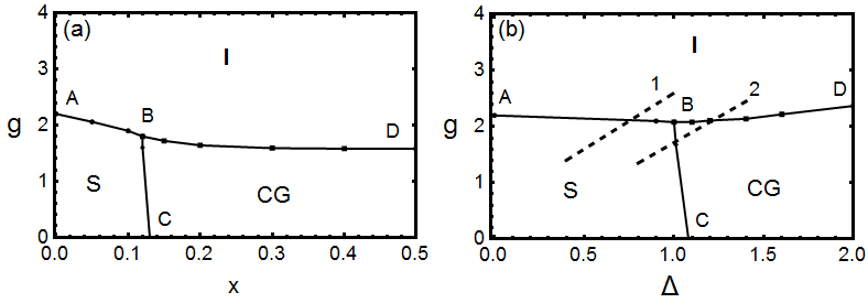
Figure 1: Phase diagrams as a function of $g=(E_{c}/E_{J})^{1/2}$ and disorder strengths $x$ or $\Delta$, showing the superconducting (S), insulating (I) and chiral-glass (CG) phases. $E_{c}$ and $E_{J}$ are the charging and Josephson-coupling energies, respectively. (a) Binary phase-glass model, where $x$ is the fraction of negative random Josephson couplings $\pm E_{J}$. (b) Gaussian phase-glass model, where $\Delta$ is the width of the Gaussian distribution of Josephson couplings with average value $E_{J}$. The dotted lines $1$ and $2$ indicate two different possible paths for the superconductor to insulator transition.

II Phase-glass models

We consider disordered superconductors described as a two-dimensional (2D) array of Josephson junctions, allowing for charging effects and gauge disorder, defined by the Hamiltonian Bradley and Doniach (1984); Fazio and van der Zant (2001); Phillips and Dalidovich (2003b); Granato (2017)

$${\cal H}={{E_{C}}\over 2}\sum_{i}n_{i}^{2}-\sum_{<ij>}E_{ij}\cos(\theta_{i}-\theta_{j}).$$ (1)

The first term in Eq. (1) describes quantum fluctuations induced by the charging energy, $E_{C}n_{i}^{2}/2$, of a non-neutral superconducting ”grain”, or ”island”, located at site $i$ of a reference square lattice, where $E_{C}=4e^{2}/C$, $e$ is the electronic charge, and $n_{i}=-i\partial/\partial\theta_{i}$ is the operator, canonically conjugate to the phase operator $\theta_{i}$, representing the deviation of the number of Cooper pairs from a constant integer value. The effective capacitance to the ground of each grain $C$ is assumed to be spatially uniform, for simplicity. The second term in (1) is the Josephson-junction coupling between nearest-neighbor grains described by phase variables $\theta_{i}$. For a spatially uniform Josephson coupling, $E_{ij}=E_{J}>0$. Equation (1) is also known as the quantum rotor model Cha et al. (1991); Sachdev (2000), with additional effects of disorder in $E_{ij}$.

The phase-glass model, as introduced by Dalidovich and PhillipsDalidovich and Phillips (2002); Phillips and Dalidovich (2003a, b) to explain the Bose metal phase of superconducting films, incorporates the effects of disorder of $E_{ij}$ in Eq. (1) due to the random location of negative Josephson coupling ($E_{ij}<0$). Assuming an asymmetric Gaussian distribution of $E_{ij}$ with nonzero zero mean, this model has been studied in detail analytically, within a mean field theory approach.

The phase-glass model can also be regarded as a quantum version of the 2D chiral glass model Kawamura and Tanemura (1991); Kawamura and Li (1997); Granato (1998), or XY spin glass Villain (1977), with varying degree of disorder, studied in the context of spin glasses and high-$T_{c}$ superconductors containing $\pi$ junctions. In the classical limit $E_{c}\rightarrow 0$, the chiral order parameter arises from the directions of the local circulating currents (Josephson vortices) introduced by the frustration effects of negative junctions. The chiral variable can be defined as

$$\chi_{p}=\frac{1}{\chi_{0}}\sum^{\prime}_{<ij>}E_{ij}\sin(\theta_{i}-\theta_{j}),$$ (2)

where the summation $\sum^{\prime}_{<ij>}$ is a direct sum around the plaquette $p$ of the lattice and $\chi_{0}$ is a normalization factor. For sufficiently large disorder, a chiral-glass phase occurs with random local circulating currents of different chiralities $\chi$. Although such a glass phase is unstable against thermal fluctuations in two dimensions Kawamura and Tanemura (1991); Granato (1998); Kosterlitz and Akino (1999), it remains stable to quantum fluctuations at zero temperature Granato (2017), below some critical value of $E_{c}$.

Since $E_{ij}<0$ is equivalent to a positive Josephson coupling $|E_{ij}|$ with a phase shift $A_{ij}=\pi$ to the phase difference $\theta_{i}-\theta_{j}$ in Eq. (1), the phase-glass model is a particular case of random gauge models Granato (2017), with a binary distribution of phase shifts $A_{ij}=0$ or $\pi$, in contrast to the gauge-glass model Kim and Stroud (2008); Tang and Chen (2008), where $A_{ij}$ has a continuous distribution.

We consider two different phase-glass models, given by asymmetric probability distributions of $E_{ij}$:

1. $P(E_{ij})=x\delta(E_{ij}+E_{J})+(1-x)\delta(E_{ij}-E_{J})$ (binary)

2. $P(E_{ij})=e^{-(E_{ij}-E_{J})^{2}/2\Delta^{2}}/\Delta\sqrt{2\pi}$ (Gaussian)

The above binary and Gaussian disorder distributions are parameterized by $x$ and $\Delta$, respectively, with an average value of the Josephson coupling $<E_{ij}>\neq 0$, except in the limit $x=0.5$ for the binary model, where $x$ corresponds to the fraction of negative Josephson junctions. Only the Gaussian phase-glass model has been studied in detail analytically, using a mean-field theory approach Dalidovich and Phillips (2002); Phillips and Dalidovich (2003a, b).

III Path-integral representation and Monte Carlo simulation

The quantum phase transition at zero temperature can be conveniently studied in the framework of the imaginary-time path-integral formulation of the model Sondhi et al. (1997); Sachdev (2000). In this representation, the 2D quantum model of Eq. (1) maps into a (2+1)D classical statistical mechanics problem. The extra dimension corresponds to the imaginary-time direction. Dividing the time axis $\tau$ into slices $\Delta\tau$, the ground state energy corresponds to the reduced free energy $F$ of the classical model per time slice. The reduced classical Hamiltonian can be written as Bradley and Doniach (1984); Wallin et al. (1994); Sondhi et al. (1997)

$$H= -\frac{1}{g}[\sum_{\tau,i}\cos(\theta_{\tau,i}-\theta_{\tau+1,i})$$ (4)

$$+\sum_{<ij>,\tau}e_{ij}\cos(\theta_{\tau,i}-\theta_{\tau,j}],$$

where $e_{ij}=E_{ij}/E_{J}$ and $\tau$ labels the sites in the discrete time direction. The ratio $g=(E_{C}/E_{J})^{1/2}$, which drives the quantum phase transition for the model of Eq. (1), corresponds to an effective ”temperature” in the (2+1)D classical model of Eq. (4). The coupling of the phases $\theta_{\tau,j}$ in the time direction results from a Villain approximation, used to obtain the phase representation of the first term in Eq. (1), but it should preserve the universal aspects of the critical behavior Sondhi et al. (1997). The classical Hamiltonian of Eq. (4) can be viewed as a 3D layered XY model, where frustration effects exist only in the 2D layers. Randomness in $e_{ij}$ corresponds to disorder completely correlated in the time direction.

Equilibrium Monte Carlo (MC) simulations are carried out using the 3D classical Hamiltonian in Eq. (4) regarding $g$ as a ”temperature”-like parameter for different values of the disorder strength $x$ or $\Delta$. The parallel tempering method Hukushima and Nemoto (1996) is used in the simulations with periodic boundary conditions, as in previous works Granato (2016a, b, 2017). Since the correlation lengths in the spatial and imaginary-time directions are related by dynamical scaling as $\xi_{\tau}\propto\xi^{z}$, the finite-size scaling analysis is performed for different linear sizes $L$ of the square lattice with the constraint $L_{\tau}=aL^{z}$, where $a$ is a constant aspect ratio. This choice simplifies the scaling analysis, otherwise an additional scaling variable $L_{\tau}/L^{z}$ would be required to describe the scaling functions. The value of $a$ is chosen to minimize the deviations of $aL^{z}$ from integer numbers. We used typically $10^{4}$ MC passes for equilibration and for calculations of average quantities. Averages over disorder used $100$ to $1000$ samples for system sizes ranging from $L=16$ to $L=30$. Equilibration was checked with the methods described in Refs. Hukushima and Nemoto, 1996; Bhatt and Young, 1988.

The MC simulations described above employing periodic boundary conditions, do not allow a direct determination of the phase stiffness of the system in the spatial direction, $\gamma_{x}$, for large disorder. The dominant effect of the gauge disorder introduces additional phase shifts, which lead to negative values of phase stiffness depending on the disorder configurations. To probe the phase stiffness in this regime, we have also employed a driven MC method with fluctuating boundary conditions Granato (2004b). For that, the layered classical model of Eq. (4) is viewed as a 3D superconductor. In the presence of an external driving perturbation $J_{x}$ (”current density”) that couples to the phase difference $\theta_{\tau,i+\hat{x}}-\theta_{\tau,i}$ along the $\hat{x}$ direction, the classical Hamiltonian of Eq. (4) is modified to

$$H_{J}=H-\sum_{i,\tau}\frac{J_{x}}{g}(\theta_{\tau,i+\hat{x}}-\theta_{\tau,i}).$$ (5)

MC simulations are carried out using the Metropolis algorithm and the time dependence is obtained from the MC time $t_{mc}$. When $J_{x}\neq 0$, the system is out of equilibrium since the total energy is unbounded. The lower-energy minima occur at phase differences $\theta_{\tau,i+\hat{x}}-\theta_{\tau,i}$, which increase with time $t_{mc}$, leading to a net phase slippage rate proportional to $V_{x}=<d(\theta_{\tau,i+\hat{x}}-\theta_{\tau,i})/dt_{mc}>$, corresponding to the average ”voltage” per unit length. The measurable quantity of interest is the phase slippage response (”nonlinear resistivity”) defined as $R_{x}=V_{x}/J_{x}$. Similarly, we define $R_{\tau}$ as the phase slippage response to the applied perturbation $J_{\tau}$ in the layered (imaginary-time) direction. One then expects that $R_{x}$ should approach a nonzero value when $J_{x}\rightarrow 0$ above the phase-coherence transition while below the transition it should approach zero if the phase stiffness is finite. From the nonlinear ”current-voltage” scaling near the transition, one can extract the critical coupling $g_{c}$, and the critical exponents Wengel and Young (1997); Granato (2004b); Lee et al. (1993); Granato (2016b, 2017).

IV Numerical results and discussion

The phase diagrams in Fig. 1, were obtained by locating the S-I and CG-I transitions from the behavior of the correlation length and phase stiffness as a function of $g$ for various fixed values of disorder strength, $x$ or $\Delta$. The S-CG transition was studied from the behavior of the correlation length as a function of disorder $x$ or $\Delta$ at fixed values of $g$. In the following subsections, we described the results for the critical behavior across the transition lines AB, BC and BD at particular values of $x$ or $\Delta$, obtained by scaling analysis of extensive MC simulations. These results are summarized in Table I. The errorbars for the critical exponents are estimated from deviations of the results obtained from different quantities.

IV.1 Superconductor to insulator transition

To locate the phase-coherence transition for a small degree of disorder, we first consider the behavior of the finite-size correlation length $\xi$, which can be defined as Ballesteros et al. (2000)

$$\xi(L,g)=\frac{1}{2\sin(k_{0}/2)}[S(0)/S(k_{0})-1]^{1/2}.$$ (6)

Here $S(k)$ is the Fourier transform of the correlation function $C(r)$ and $k_{0}$ is the smallest nonzero wave vector. For $g>g_{c}$, this definition corresponds to a finite-difference approximation to the infinite system correlation length $\xi(g)^{2}=-\frac{1}{S(k)}\frac{\partial S(k)}{\partial k^{2}}|_{k=0}$, taking into account the lattice periodicity. The correlation function in the spatial direction is obtained as

$$C(r)=\frac{1}{L^{2}L_{\tau}}\sum_{\tau,j}<\psi_{\tau,j}\psi_{\tau,j+r}>,$$ (7)

where $\psi_{\tau,j}=\exp(i\theta_{\tau,j})$ is the order parameter. Analogous expressions are used for the correlation function $C_{\tau}(r)$ and correlation length $\xi_{\tau}(L,g)$ in the time direction. For a continuous transition, $\xi(L,g)$ should satisfy the scaling form

$$\xi/L=F(L^{1/\nu}\delta g),$$ (8)

where $F(x)$ is a scaling function, $\delta g=g-g_{c}$ and $\nu$ is the correlation-length critical exponent. This scaling form implies that data for the ratio $\xi(L,g)/L$ as a function of $g$, for different system sizes $L$, should cross at the critical coupling $g_{c}$. Moreover, a scaling plot in the form $\xi/L\times L^{1/\nu}\delta g$ sufficiently close to $g_{c}$ should collapse the data on to the same curve.

Figure 2a shows the behavior of the correlation lengths $\xi_{\tau}$ and $\xi$ in the time and spatial directions, for the binary phase-glass model with the dynamic exponent set to $z=1.1$. The curves for $\xi_{\tau}/L$ as a function of $g$ at a fixed value of disorder $x=0.05$ for different system sizes cross approximately at the same point, providing evidence of a continuous transition. In Fig. 2b, a scaling plot according to Eq. (8) is shown, obtained by adjusting the parameters $g_{c}$ and $\nu$ to obtain the best data collapse. Figs. 2c and 2d show the corresponding behavior for the correlation length in the spatial direction. The estimate $z=1.1$ was obtained by repeating the calculations for different values of $z$ larger than $z=1$ and choosing the one that gives the best data collapse. Similar results are obtained for the Gaussian phase-glass model as shown in Fig. 3.

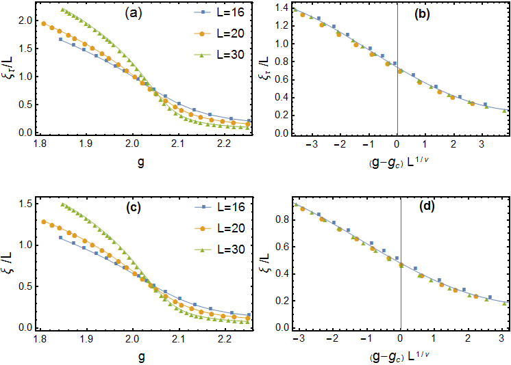
Figure 2: (a) Correlation length in the imaginary time direction $\xi_{\tau}$ of the binary phase-glass model near the S-I transition at $x=0.05$ for different system sizes $L$ and (b) corresponding scaling plot of the data near the transition with $g_{c}=2.048$, $\nu=0.85$. (c) Correlation length in the spatial direction $\xi$ and (d) corresponding scaling plot with $g_{c}=2.05$, $\nu=0.89$. $L_{\tau}=aL^{z}$, with aspect ratio $a=0.641$ and $z=1.1$

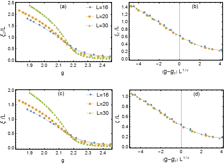
Figure 3: (a) Same as Fig. 2a but for the Gaussian phase-glass model at $\Delta=0.5$ and (b) corresponding scaling plot with $g_{c}=2.177$, $\nu=0.86$. (c) Correlation length in the spatial direction $\xi$ and (d) corresponding scaling plot with $g_{c}=2.18$, $\nu=0.86$.

The phase-coherence transition described above can be identified as a superconductor-insulator transition from the behavior of the phase stiffness $\gamma$, which measures the free energy cost to impose an infinitesimal phase twist along a certain direction. In the imaginary time direction, $\gamma_{\tau}$, which corresponds to the compressibility of the bosonic system, is given by Cha and Girvin (1994); Wallin et al. (1994)

$$\gamma_{\tau}=\frac{1}{L^{2}L_{\tau}g^{2}}[g<\epsilon_{\tau}>-<I_{\tau}^{2}>+<I_{\tau}>^{2}]_{d},$$ (9)

where $\epsilon_{\tau}=\sum_{\tau,i}\cos(\theta_{\tau,i}-\theta_{\tau+1,i})$ and $I_{\tau}=\sum_{\tau,i}\sin(\theta_{\tau,i}-\theta_{\tau+1,i})$. In Eq. (9), $<\ldots>$ represents a MC average for a fixed disorder configuration, and $[\ldots]_{d}$ represents an average over different disorder configurations. Similarly, the phase stiffness in the spatial direction, $\gamma_{x}$, which corresponds to the superfluid density, is given by the analogous expression in the $\hat{x}$-direction. In the superconducting phase, $\gamma$ should be finite, reflecting the existence of phase coherence, while in the insulating phase it should vanish in the thermodynamic limit. For a continuous phase transition, $\gamma_{\tau}$ should satisfy the finite-size scaling form Wallin et al. (1994)

$$\gamma_{\tau}L^{2-z}=F(L^{1/\nu}\delta g),$$ (10)

where $F(x)$ is a scaling function and $\delta g=g-g_{c}$. This scaling form implies that data for $\gamma_{\tau}L^{2-z}$ as a function of $g$, for different system sizes $L$, should cross at the critical coupling $g_{c}$. Fig. 4a shows this crossing behavior and Fig. 4b shows the corresponding scaling plot of the data according to the scaling form of Eq. (10). The same behavior is found for the Gaussian phase-glass model as shown in Fig. 5.

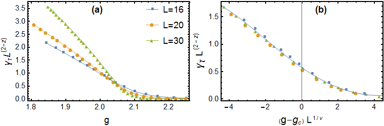
Figure 4: (a) Phase stiffness in the imaginary time direction $\gamma_{\tau}$ of the binary phase-glass model near the S-I transition at $x=0.05$ for different system sizes $L$ and (b) corresponding scaling plot with $g_{c}=2.05$ and $\nu=0.82$.

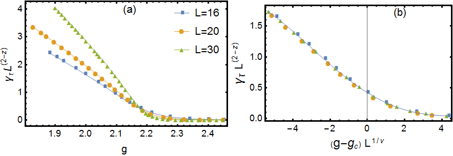
Figure 5: (a) Same as Fig. 4a but for the Gaussian phase-glass model at $\Delta=0.5$ and (b) corresponding scaling plot with $g_{c}=2.178$ and $\nu=0.84$.

Another quantity characterizing the superconductor to insulator transition is the electrical conductivity at the transition. Its value should be universal, it does not depend on the parameters of the model, but it can depend on the universality class of the transition Fisher et al. (1990). Following the scaling method described by Cha et al. Cha and Girvin (1994); Cha et al. (1991), the universal conductivity can be determined from the frequency and finite-size dependence of the phase stiffness $\gamma(w)$ in the spatial direction. The conductivity is given by the Kubo formula

$$\sigma=2\pi\sigma_{Q}\lim_{w_{n}\rightarrow 0}\frac{\gamma(iw_{n})}{w_{n}},$$ (11)

where $\sigma_{Q}=(2e)^{2}/h$ is the quantum of conductance and $\gamma(iw_{n})$ is a frequency dependent phase stiffness evaluated at the finite frequency $w_{n}=2\pi n/L_{\tau}$, with $n$ an integer. The frequency dependent phase stiffness in the $\hat{x}$ direction is given by

$$\gamma(i\omega_{n})=\frac{1}{L^{2}L_{\tau}g^{2}}[ g <\epsilon_{x}>-<|I(iw_{n})|^{2}>$$ (12)

$$+ <|I(iw_{n})|>^{2}]_{d},$$ (13)

where

$$\epsilon_{x} = \sum_{\tau,j}e_{j,j+\hat{x}}\cos(\Delta_{x}\theta_{\tau,j}),$$ (14)

$$I(iw_{n}) = \sum_{\tau,j}e_{j,j+\hat{x}}\sin(\Delta_{x}\theta_{\tau,j})e^{iw_{n}\tau},$$ (15)

and $\Delta_{x}\theta_{\tau,j}=\theta_{\tau,j}-\theta_{\tau,j+\hat{x}}$. At the transition, $\gamma(iw_{n})$ vanishes linearly with frequency and $\sigma$ assumes a universal value $\sigma^{*}$, which can be extracted from its frequency and finite-size dependence as Cha and Girvin (1994)

$$\frac{\sigma(iw_{n})}{\sigma_{Q}}=\frac{\sigma*}{\sigma_{Q}}-c(\frac{w_{n}}{2\pi}-\alpha\frac{2\pi}{w_{n}L_{\tau}})\cdots$$ (16)

The parameter $\alpha$ is determined from the best data collapse of the frequency dependent curves for different systems sizes in a plot of $\frac{\sigma(iw_{n})}{\sigma_{Q}}$ versus $x_{o}=(\frac{w_{n}}{2\pi}-\alpha\frac{2\pi}{w_{n}L_{\tau}})$. The universal conductivity is obtained from the intercept of these curves with the line $x_{o}=0$. From this scaling behavior, shown in Fig. 6a for the binary phase glass model and Fig. 6b for the Gaussian phase-glass model, we obtain at the S-I transition $\sigma^{*}/\sigma_{Q}=0.32(3)$ and $\sigma^{*}/\sigma_{Q}=0.31(3)$, respectively.

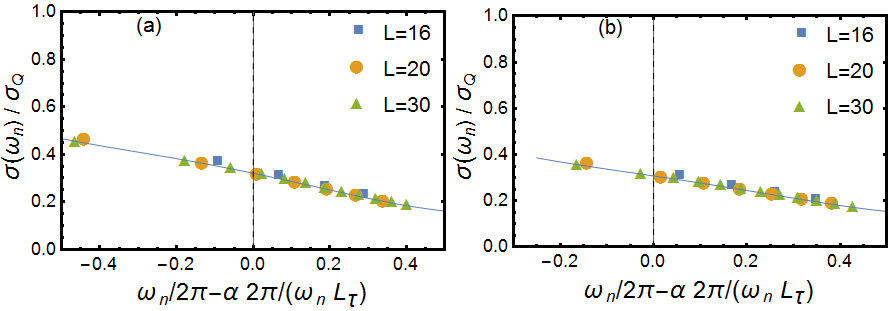
Figure 6: Scaling plot of conductivity $\sigma(iw_{n})$ at the critical coupling $g_{c}$ for (a) the binary phase-glass model at $x=0.05$, $g_{c}=2.058$ with $\alpha=0.5$ and (b) the Gaussian phase-glass model at $\Delta=0.5$, $g_{c}=2.187$ with $\alpha=0.2$. The universal conductivity is given by the intercept with the $x_{o}=0$ dashed line, leading to the corresponding estimates (a) $\frac{\sigma^{*}}{\sigma_{Q}}=0.32(3)$ and (b) $\frac{\sigma^{*}}{\sigma_{Q}}=0.31(3)$.

IV.2 Superconductor to chiral-glass transition

Above a disorder-strength threshold $x_{B}$, the finite-size correlation length $\xi(L,g)$ defined in Eq. (6) no longer displays a crossing behavior at some critical $g_{c}$, indicating the absence of long-range or quasi-long range order in terms of the order parameter $\psi_{\tau,j}=\exp(i\theta_{\tau,j})$. From this change of behavior, we estimate the location of the multicritical point B at $(g_{B},x_{B})$ for the binary phase-glass model in the phase diagram of Fig. 1a and, similarly, for the Gaussian phase-glass model at $(g_{B},\Delta_{B})$ in Fig. 1b.

The superconductor to chiral glass transition can be determined from the behavior of the correlation length as a function of disorder at a fixed value of $g<g_{B}$. Figure 7a shows the behavior of the correlation length $\xi(x,L)$ for increasing disorder $x$ at $g=1.6$, for the binary phase-glass model. The curves of $\xi(x,L)/L$ for different system sizes cross approximately at the same point $x_{c}$, providing evidence of a continuous S-CG transition. In Fig.7b, a scaling plot according to Eq. (8) is shown, obtained by adjusting the parameters $x_{c}$ and $\nu$ to obtain the best data collapse. The dynamic exponent $z=1.1$ was obtained by repeating the calculations for different values larger than $z=1$ and choosing the one that gives the best data collapse. Similar results are obtained for the Gaussian phase-glass model as shown in Fig. 8.

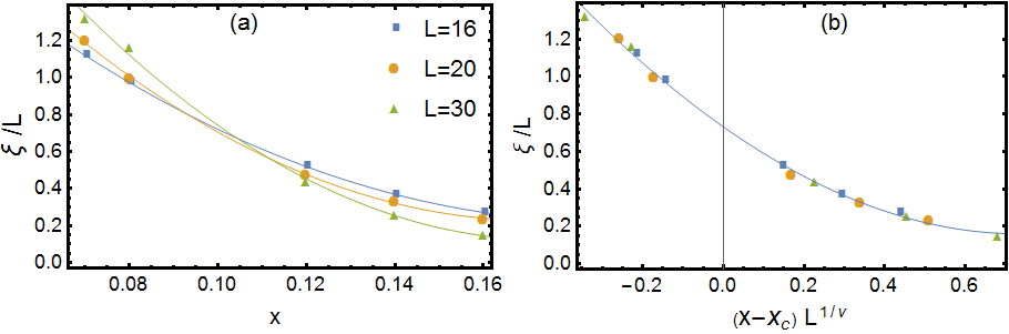
Figure 7: (a) Correlation length in the spatial direction $\xi$ of the binary phase-glass model near the S-CG transition at fixed $g=1.6$ for different system sizes $L$ and (b) corresponding scaling plot of the data near the transition with $x_{c}=0.1$, $\nu=1.4$.

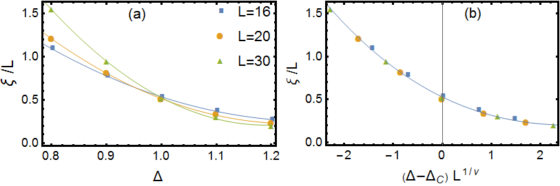
Figure 8: (a) Same as Fig. 7a but for the Gaussian phase-glass model near the S-CG transition at fixed $g=1.68$ for different system sizes $L$ and (b) corresponding scaling plot of the data near the transition with $\Delta_{c}=1.0$, $\nu=1.4$.

Point C in the phase diagrams of Fig. 1 corresponds to the superconductor to chiral-glass threshold in the limit $g\rightarrow 0$. It can be estimated from the finite-size behavior of the domain wall energy Bray and Moore (1984); Benakli et al. (1998) in the ground-state of the 3D classical model of Eq. (4). A domain wall in the finite system can be introduced by imposing antiperiodic boundary conditions in one of the spatial directions. The domain-wall energy $E_{W}(L)$ is a measure of phase coherence, and is related to the renormalized stiffness constant $\gamma_{x}(L)=E_{W}(L)/(2\pi^{2}L_{\tau})$. Although $E_{W}(L)$ fluctuates between samples with different disorder configurations, stability of the ground state with long-range order in $\psi_{\tau,j}=\exp(i\theta_{\tau,j})$ requires that the disorder average $[E_{W}]_{d}$ increases with $L$ or remains constant. We have determined numerically the change $E_{W}(L)$ in the ground-state energy of small systems by MC simulated annealing for a large number of samples. Figure 9 shows the behavior of the $[E_{W}]_{d}$ for different system sizes and increasing disorder, for both phase-glass models. For small disorder strength, it increases with $L$, indicating the existence of long-range phase coherence. For sufficiently large disorder it clearly decreases for increasing $L$, indicating a disordered glass phase. The change in the behavior yields the estimates of the chiral-glass disorder thresholds $x_{C}=0.11(2)$ and $\Delta_{C}=1.1(2)$, for the binary and Gaussian phase-glass models, respectively.

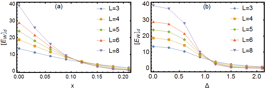
Figure 9: Domain-wall energy $[E_{W}]_{d}$ for the (a) binary and (b) Gaussian phase-glass models in the limit $g\rightarrow 0$ for increasing disorder ($x$ or $\Delta$) and different systems sizes $L$. The common crossing point of the curves gives an estimate of the chiral-glass disorder threshold $x_{C}$ and $\Delta_{C}$ in the phase diagrams of Fig. 1.

IV.3 Chiral glass to insulator transition

In the chiral-glass phase for $x>x_{B}$ or $\Delta>\Delta_{B}$ in Fig. 1, there is no long-range order in terms of the order parameter $\psi_{\tau,j}=\exp(i\theta_{\tau,j})$. It is then convenient to define a glass correlation function in terms of the overlap order parameter Bhatt and Young (1988); Rieger and Young (1994) of phase variables $q_{\tau,j}=\exp(i(\theta^{1}_{\tau,j}-\theta^{2}_{\tau,j}))$, where $1$ and $2$ label two different copies of the system with the same coupling parameters. The glass correlation function in the spatial direction is then obtained as

$$C(r)=\frac{1}{L^{2}L_{\tau}}\sum_{\tau,j}<q_{\tau,j}q_{\tau,j+r}>,$$ (17)

with the corresponding phase correlation length $\xi_{G}$ defined as in Eq. (6). Analogous expressions are used for the correlation length in the time direction $\xi_{G,\tau}$. Similarly, we can also define a chiral correlation length $\xi^{c}_{G}$ in terms of the overlap of the chiral variables of Eq. (2), $q^{c}_{\tau,p}=\chi^{1}_{\tau,p}\ \chi^{2}_{\tau,p}$.

Figure 10 shows the behavior of the correlation length $\xi_{G,\tau}$ and $\xi_{G}$ in the time and spatial directions, for the binary phase-glass model at $x=0.2$. The dynamic exponent is set to $z=1.2$, the same value estimated for the symmetric models Granato (2017). We find that this value gives consistent results for the scaling behavior and also agrees with independent estimates of $z$ using large systems, as will be described further ahead. As shown in Fig. 10a, the curves for $\xi_{G,\tau}/L$ as a function of $g$ for different system sizes cross approximately at the same point $g_{c}$, providing evidence of a continuous CG-I transition. Fig. 10b, shows the scaling plot according to Eq. (8) providing estimates for $g_{c}$ and $\nu$. Figs. 10c and 10d shows the corresponding behavior for the correlation length in the spatial direction. The results for the chiral correlation length $\xi^{c}_{G}$ are shown in Figure 11. The behavior is essentially the same but the data are much noisier. Similar results are obtained for the Gaussian phase-glass model as shown in Fig. 12 and 13.

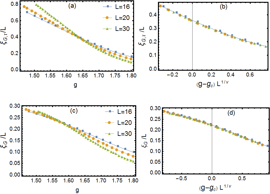
Figure 10: (a) Correlation length in the imaginary time direction $\xi_{G,\tau}$ of the binary phase-glass model near the CG-I transition at $x=0.2$ for different system sizes $L$ and (b) corresponding scaling plot of the data near the transition with $g_{c}=1.655$, $\nu=1.6$. (c) Correlation length in the spatial direction $\xi_{G}$ and (d) corresponding scaling plot with $g_{c}=1.59$, $\nu=1.6$. $L_{\tau}=aL^{z}$, with aspect ratio $a=0.642$ and $z=1.2$

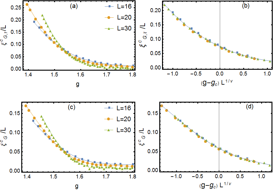
Figure 11: (a) Chiral correlation length in the imaginary time direction $\xi^{c}_{G,\tau}$ of the binary phase-glass model near the CG-I transition at $x=0.2$ for different system sizes $L$ and (b) corresponding scaling plot of the data near the transition with $g_{c}=1.54$, $\nu=1.3$. (c) Correlation length in the spatial direction $\xi^{c}_{G}$ and (d) corresponding scaling plot with $g_{c}=1.53$, $\nu=1.3$. $L_{\tau}=aL^{z}$, with aspect ratio $a=0.642$ and $z=1.2$

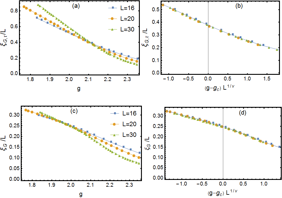
Figure 12: (a) Same as Fig. 10 but for the Gaussian phase-glass model at $\Delta=1.6$ and (b) corresponding scaling plot of the data near the transition with $g_{c}=2.123$, $\nu=1.36$. (c) Correlation length in the spatial direction $\xi_{G}$ and (d) corresponding scaling plot with $g_{c}=2.0$, $\nu=1.7$.

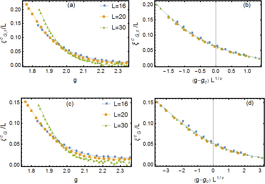
Figure 13: (a) Same as Fig. 11 but for the Gaussian phase-glass model at $\Delta=1.6$ and (b) corresponding scaling plot of the data near the transition with $g_{c}=1.978$, $\nu=1.3$. (c) Correlation length in the spatial direction $\xi^{c}_{G}$ and (d) corresponding scaling plot with $g_{c}=1.963$, $\nu=1.03$.

In Fig. 14, we show the behavior of the phase stiffness in the time direction. Curves for different system sizes cross approximately at the same critical coupling $g_{c}$ and the corresponding scaling plot of the data according to the scaling form of Eq. 10 provide alternative estimates of $g_{c}$ and $\nu$. The same behavior is found for the Gaussian phase-glass model as shown in Figs. 15.

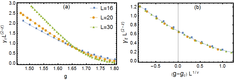
Figure 14: (a) Phase stiffness in the imaginary time direction $\gamma_{\tau}$ for the binary phase-glass model near the CG-I transition at $x=0.2$ for different system sizes $L$ and (b) corresponding scaling plot with $g_{c}=1.675$ and $\nu=1.2$.

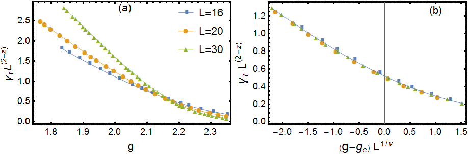
Figure 15: (a) Same as Fig. 14 but for the Gaussian phase-glass at $\Delta=1.6$ and (b) corresponding scaling plot with $g_{c}=2.176$ and $\nu=1.21$.

It should be noted that there are significant discrepancies in the critical couplings obtained from the scaling behavior of the correlations lengths $\xi_{G}$, $\xi^{c}_{G}$ and phase stiffness $\gamma_{\tau}$, for both models. They are likely to result from different corrections to finite-size scaling and we thus assume they represent estimates of the same CG-I transition, where the phase-coherence transition is accompanied by a chiral transition and described by a single divergent length scale.

The scaling behavior described above for the correlation $\xi_{G}$ and phase stiffness $\gamma_{\tau}$ already indicates phase coherence below the CG-I transition and, therefore, the chiral-glass phase is expected to be superconducting. To further investigate the superconducting properties of this phase, we need to look at the phase stiffness in the spatial direction. Unfortunately, the dominant effect of the gauge disorder leads to negative values for the phase stiffness Huse and Seung (1990); Kosterlitz and Akino (1999) when obtained directly, as in Eq. (9), depending on the disorder configurations. It turns out, however, that the frequency-dependent phase stiffness $\gamma(i\omega)$ defined in Eq. (13) is well behaved for nonzero frequencies $\omega$. Its scaling behavior at small frequencies determines the electrical conductivity from the Kubo formula (Eq. 11). If $\gamma(i\omega)$ is finite when $\omega\rightarrow 0$ in the chiral-glass phase then $\sigma$ diverges and this phase is superconducting. Near the CG-I transition, it should therefore satisfy the scaling relation Cha et al. (1991); Wallin et al. (1994)

$$\gamma(i\omega_{n})/\omega_{n}=F_{\pm}(\omega_{n}\xi^{z}),$$ (18)

in the absence of finite size effects. The + and - signs correspond to $g>g_{c}$ and $g<g_{c}$. Indeed, as shown in Fig. 16 for the binary and in Fig. 17 for the Gaussian phase-glass models, the phase stiffness $\gamma(i\omega_{n})$ at low frequencies and different couplings $g$ for a large system where finite-size effects are small satisfy the above scaling form, providing evidence for a phase transition from a superconducting chiral glass to insulator transition.

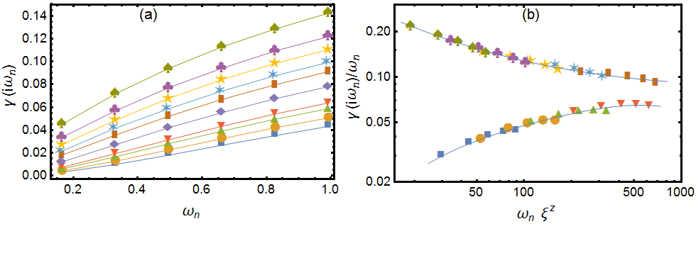
Figure 16: (a) Phase stiffness $\gamma(i\omega)$ for the binary phase-glass model near the CG-I transition at $x=0.2$, for different couplings $g$ with $L=30$. From the top bottom: $g=1.50,1.55,1.58,1.61,1.63,1.67,1.71,1.73,1.76$ and $1.80$. (b) Scaling plot with $\xi=|g/g_{c}-1|^{-\nu}$ for $g_{c}=1.672$ and $z\nu=1.75$.

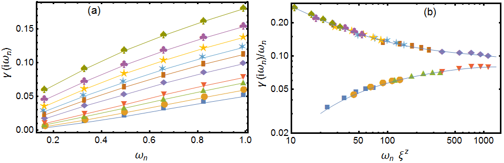
Figure 17: (a) Same as Fig. 16 but for the Gaussian phase-glass model at $\Delta=1.6$. From the top bottom: $g=1.84,1.92,1.97,2.02,2.06,2.11,2.19,2.23,2.29$ and $2.35$. (b) Scaling plot with $\xi=|g/g_{c}-1|^{-\nu}$ for $g_{c}=2.15$ and $z\nu=1.8$.

To further verify the finite phase stiffness of the chiral-glass phase and obtain an independent estimate of $z$, we have also studied the scaling behavior of the phase slippage response (”nonlinear resistivity”) $R_{x}=V_{x}/J_{x}$, obtained by driven MC dynamics Granato (2004b, 2017) as described in Sec. III. As shown in the Appendix, the scaling analysis is consistent with the above results obtained from $\xi_{G}$ and $\gamma(i\omega)$ scaling and therefore provide further support for the finite phase stiffness and a superconducting chiral-glass phase.

Since we have found that the chiral-glass phase is superconducting, it is interesting to obtain an estimate of the conductivity $\sigma^{*}$ at the CG-I transition. Following the scaling method of Cha et al. Cha and Girvin (1994); Cha et al. (1991) described in Sec. IV.1, $\sigma^{*}$ can be determined from a scaling plot according to Eq. (16). Fig. 18a shows this scaling plot for the binary phase glass model and Fig. 18b for the Gaussian phase-glass model, from which we estimate at the CG-I transition $\sigma^{*}/\sigma_{Q}=0.55(3)$ and $\sigma^{*}/\sigma_{Q}=0.59(3)$, respectively.

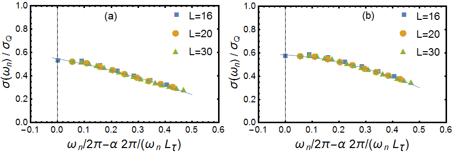
Figure 18: Scaling plot of conductivity $\sigma(iw_{n})$ at the critical coupling $g_{c}$ for (a) the binary phase-glass model at $x=0.2$, $g_{c}=1.672$ and (b) the Gaussian phase-glass model at $\Delta=1.6$, $g_{c}=2.15$ with $\alpha=0.06$. The universal conductivity is given by the intercept with the $x_{o}=0$ dashed line, leading to the corresponding estimates (a) $\frac{\sigma^{*}}{\sigma_{Q}}=0.55(3)$ and (b) $\frac{\sigma^{*}}{\sigma_{Q}}=0.59(3)$.

	binary model
	S-I	CG-I	S-CG
$x_{c},g_{c}$	$0.05,2.049(1)$	$0.2,1.64(4)$	$0.10(2),1.6$
$z$	$1.10(5)$	$1.2(1)$	$1.1(1)$
$\nu$	$0.85(2)$	$1.5(2)$	$1.5(3)$
$\sigma^{*}/\sigma_{Q}$	$0.32(3)$	$0.55(3)$	-

	Gaussian model
	S-I	CG-I	S-CG
$\Delta_{c},g_{c}$	$0.5,2.178(1))$	$1.6,2.10(5)$	$1.00(2),1.68$
$z$	$1.10(5)$	$1.2(1)$	$1.1(1)$
$\nu$	$0.85(2)$	$1.4(2)$	$1.4(3)$
$\sigma^{*}/\sigma_{Q}$	$0.31(3)$	$0.59(3)$	-

Table 1: Critical couplings $(x_{c},g_{c})$ or $(\Delta_{c},g_{c})$, exponents $z,\nu$ and conductivity $\sigma^{*}$ at the transition of the S-I, CG-I and S-CG transitions in the phase diagrams of Fig. 1, for the binary and Gaussian phase-glass models. At the S-CG transition $\sigma$ remains infinity.

V Summary and Conclusions

We have studied the superconductor to insulator transition in two-dimensional phase-glass (or chiral-glass) models with varying degree of disorder by path-integral MC simulations and finite-size scaling. Two different models were considered, with binary and Gaussian distribution of quenched disorder, having nonzero mean. Both models display the same topology of the phase diagram (Fig. 1) with critical exponents that agree within the estimated errorbars (Table I). In addition to the usual superconducting and insulating phases, a chiral-glass phase occurs for sufficiently large disorder. The chiral-glass to insulator transition is in a different universality class, with critical exponents and universal conductivity at the transition significantly different from those of the superconductor-insulator transition for small disorder.

The transition from superconductor to insulator can take place via the intermediate chiral-glass phase, depending on the parameters of the models. We find, however, that the chiral-glass phase has a finite phase stiffness, being still a superconductor, instead of the Bose metal, which has been suggested by the mean-field theory approach Dalidovich and Phillips (2002); Phillips and Dalidovich (2003a, b). This indicates that the 2D phase-glass model does not provide a theoretical framework for the Bose metal state in the zero temperature limit observed experimentally Jaeger et al. (1989); Yazdani and Kapitulnik (1995); Chervenak and Valles Jr (2000); Christiansen et al. (2002); Tsen et al. (2016), at least in its simplest form with onsite charging energy, short-range Josephson interactions, and an absence of magnetic screening effects.

Our results are also relevant for superconducting thin films nanostructured with a periodic pattern of nanoholes and doped with magnetic impurities Zhang et al. (2019). Assuming that these magnetic impurities introduce $\pi$ junctions Bulaevskii et al. (1977) distributed randomly, the transition to the insulating phase for sufficient large impurity doping should be in the universality class of the chiral-glass to insulator transition studied here. The disappearance of magnetic frustration effects for the activation energy in the insulating phase at large doping Zhang et al. (2019), is in fact consistent with such a chiral-glass regime.

VI Appendix

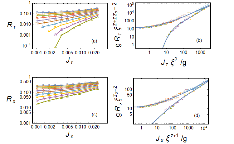
Figure 19: Scaling behavior of the phase slippage response for the binary phase-glass model near the CG-I transition at $x=0.2$ for $L=60$ in (a) the imaginary-time direction $R_{\tau}$ and (c) spatial direction $R_{x}$ near the CG-I transition. From the top down, the couplings are $g=1.80,1.78,1.76,1.74,1.72,1.70,1.68,1.66,1.64$ and $1.62$. (b) and (d) Scaling plots corresponding to (a) and (c), respectively, for data near the transition with $\xi=|g/g_{c}-1|^{-\nu}$ using the same parameters $g_{c}=1.67$, $z_{o}=2.3$, $z=1.25$, and $\nu=1.2$.

Here we consider the scaling behavior of the phase slippage response (”nonlinear resistivity”) $R_{x}=V_{x}/J_{x}$ near the CG-I transition, obtained by driven MC dynamics Granato (2004b, 2017) as described in Sec. III. If the phase stiffness is finite in the chiral-glass phase, we then expects that $R_{x}$ should approach a nonzero value when $J_{x}\rightarrow 0$ above the transition, $g>g_{c}$, while below the transition it should approach zero. From the nonlinear scaling behavior near the transition Granato (2017); Lee et al. (1993) of a sufficiently large system, one can also extract the critical coupling $g_{c}$, and the critical exponents $\nu$ and $z$. Figs. 19 shows the behavior of the nonlinear phase slippage response $R_{x}$ and $R_{\tau}$ for the binary phase-glass model as a function of the applied perturbation $J_{x}$ and $J_{\tau}$, respectively. The behavior for different values of $g$ is consistent with a phase-coherence transition at an apparent critical coupling in the range $g_{c}\sim 1.68-1.66$. For $g>g_{c}$, both $R_{x}$ and $R_{\tau}$ tend to a finite value while for $g<g_{c}$, they extrapolate to low values. Assuming the transition is continuous, the nonlinear response behavior sufficiently close to the transition should satisfy a scaling form in terms of $J_{x}$, $J_{\tau}$ and $g$. The critical coupling $g_{c}$ and critical exponents $\nu$ and $z$ can then be obtained from the best data collapse satisfying the scaling behavior close to the transition. $R_{x}$ and $R_{\tau}$ should satisfy the scaling forms Lee et al. (1993),

$$gR_{x}\xi^{z_{0}-z} = F_{\pm}(J_{x}\xi^{z+1}/g),$$ (19)

$$gR_{\tau}\xi^{z+z_{0}z-2} = H_{\pm}(J_{\tau}\xi^{2}/g),$$ (20)

where $z_{o}$ is an additional critical exponent describing the MC relaxation times, $t^{r}_{mc,x}\sim\xi^{z_{o}}$ and $t^{r}_{mc,\tau}\sim\xi_{\tau}^{z_{o}}$, in the spatial and imaginary-time directions, respectively, and $\xi=|g/g_{c}-1|^{-\nu}$. The + and - signs correspond to $g>g_{c}$ and $g<g_{c}$. The joint scaling plots according to Eqs. (20) are shown in Figs. 19b and 19d, obtained by adjusting the unknown parameters. This scaling analysis gives the estimates $g_{c}=1.670(5)$, $\nu=1.10(5)$ and $z=1.25(5)$, which are consistent with the results from the correlation-length scaling described in Sec. IV.3 and therefore provide further support for the finite phase stiffness of the chiral glass phase.

References

- Fisher (1989) M. P. A. Fisher, Phys. Rev. Lett. 62, 1415 (1989).
- Huse and Seung (1990) D. A. Huse and H. S. Seung, Phys. Rev. B 42, 1059 (1990).
- Bulaevskii et al. (1977) L. Bulaevskii, V. Kuzii, and A. Sobyanin, JETP lett 25, 290 (1977).
- Spivak and Kivelson (1991) B. I. Spivak and S. A. Kivelson, Phys. Rev. B 43, 3740 (1991).
- Sigrist and Rice (1995) M. Sigrist and T. M. Rice, Rev. Mod. Phys. 67, 503 (1995).
- Kusmartsev (1992) F. V. Kusmartsev, Phys. Rev. Lett. 69, 2268 (1992).
- Kawamura (1995) H. Kawamura, Journal of the Physical Society of Japan 64, 711 (1995).
- Kawamura and Li (1997) H. Kawamura and M. Li, Phys. Rev. Lett. 78, 1556 (1997).
- Granato (2004a) E. Granato, Phys. Rev. B 69, 012503 (2004a).
- Dalidovich and Phillips (2002) D. Dalidovich and P. Phillips, Physical Review Letters 89, 027001 (2002).
- Phillips and Dalidovich (2003a) P. Phillips and D. Dalidovich, Physical Review B 68, 104427 (2003a).
- Phillips and Dalidovich (2003b) P. Phillips and D. Dalidovich, Science 302, 243 (2003b).
- Yazdani and Kapitulnik (1995) A. Yazdani and A. Kapitulnik, Physical review letters 74, 3037 (1995).
- Chervenak and Valles Jr (2000) J. Chervenak and J. Valles Jr, Physical Review B 61, R9245 (2000).
- Jaeger et al. (1989) H. Jaeger, D. Haviland, B. Orr, and A. Goldman, Physical Review B 40, 182 (1989).
- Christiansen et al. (2002) C. Christiansen, L. Hernandez, and A. Goldman, Physical Review Letters 88, 037004 (2002).
- Das and Doniach (1999) D. Das and S. Doniach, Physical Review B 60, 1261 (1999).
- Granato (1998) E. Granato, Phys. Rev. B 58, 11161 (1998).
- Lee and Young (2003) L. W. Lee and A. P. Young, Phys. Rev. Lett. 90, 227203 (2003).
- Villain (1977) J. Villain, Journal of Physics C: Solid State Physics 10, 4793 (1977).
- Kawamura and Tanemura (1991) H. Kawamura and M. Tanemura, J. Phys. Soc. Jpn. 60, 608 (1991).
- Kosterlitz and Akino (1999) J. M. Kosterlitz and N. Akino, Phys. Rev. Lett. 82, 4094 (1999).
- Granato (2017) E. Granato, Phys. Rev. B 96, 184510 (2017).
- Zhang et al. (2019) X. Zhang, J. C. Joy, C. Wu, J. H. Kim, J. Xu, and J. M. Valles Jr, Physical Review Letters 122, 157002 (2019).
- Granato (2016a) E. Granato, Eur. Phys. J. B 89, 68 (2016a).
- Granato (2016b) E. Granato, Phys. Rev. B 94, 060504(R) (2016b).
- Wu and Phillips (2006) J. Wu and P. Phillips, Physical Review B 73, 214507 (2006).
- Tsen et al. (2016) A. Tsen, B. Hunt, Y. Kim, Z. Yuan, S. Jia, R. Cava, J. Hone, P. Kim, C. Dean, and A. Pasupathy, Nature Physics 12, 208 (2016).
- Phillips (2016) P. W. Phillips, Nature Physics 12, 206 (2016).
- Bradley and Doniach (1984) R. M. Bradley and S. Doniach, Phys. Rev. B 30, 1138 (1984).
- Fazio and van der Zant (2001) R. Fazio and H. van der Zant, Phys. Rep. 355, 235 (2001).
- Cha et al. (1991) M.-C. Cha, M. P. A. Fisher, S. M. Girvin, M. Wallin, and A. P. Young, Phys. Rev. B 44, 6883 (1991).
- Sachdev (2000) S. Sachdev, Quantum Phase Transitions (Cambridge University Press, 2000).
- Kim and Stroud (2008) K. Kim and D. Stroud, Phys. Rev. B 78, 174517 (2008).
- Tang and Chen (2008) L.-H. Tang and Q.-H. Chen, Journal of Statistical Mechanics: Theory and Experiment 2008, P04003 (2008).
- Sondhi et al. (1997) S. L. Sondhi, M. Girvin, J. Carini, and D. Sahar, Rev. Mod. Phys. 69, 315 (1997).
- Wallin et al. (1994) M. Wallin, E. S. Sorensen, S. M. Girvin, and A. P. Young, Phys. Rev. B 49, 12115 (1994).
- Hukushima and Nemoto (1996) K. Hukushima and K. Nemoto, J. Phys. Soc. Jpn. 65, 1604 (1996).
- Granato (2004b) E. Granato, Phys. Rev. B 69, 144203 (2004b).
- Wengel and Young (1997) C. Wengel and A. P. Young, Phys. Rev. B 56, 5918 (1997).
- Lee et al. (1993) K. H. Lee, D. Stroud, and S. Girvin, Phys. Rev. B 48, 1233 (1993).
- Ballesteros et al. (2000) H. G. Ballesteros, A. Cruz, L. A. Fenández, V. Martin-Mayor, J. Pech, J. J. Ruiz-Lorenzo, A. Tarancón, P. Téllez, C. L. Ullod, and C. Ungil, Phys. Rev. B 62, 14237 (2000).
- Cha and Girvin (1994) M.-C. Cha and S. M. Girvin, Phys. Rev. B 49, 9794 (1994).
- Fisher et al. (1990) M. P. A. Fisher, G. Grinstein, and S. M. Girvin, Phys. Rev. Lett. 64, 587 (1990).
- Bray and Moore (1984) A. Bray and M. Moore, Journal of Physics C: Solid State Physics 17, L463 (1984).
- Benakli et al. (1998) M. Benakli, E. Granato, S. R. Shenoy, and M. Gabay, Phys. Rev. B 57, 10314 (1998).
- Bhatt and Young (1988) R. N. Bhatt and A. P. Young, Phys. Rev. B 37, 5606 (1988).
- Rieger and Young (1994) H. Rieger and A. P. Young, Physical Review Letters 72, 4141 (1994).