Unsupervised Embedding of Hierarchical Structure
in Euclidean Space

Abstract

Deep embedding methods have influenced many areas of unsupervised learning. However, the best methods for learning hierarchical structure use non-Euclidean representations, whereas Euclidean geometry underlies the theory behind many hierarchical clustering algorithms. To bridge the gap between these two areas, we consider learning a non-linear embedding of data into Euclidean space as a way to improve the hierarchical clustering produced by agglomerative algorithms. To learn the embedding, we revisit using a variational autoencoder with a Gaussian mixture prior, and we show that rescaling the latent space embedding and then applying Ward’s linkage-based algorithm leads to improved results for both dendrogram purity and the Moseley-Wang cost function. Finally, we complement our empirical results with a theoretical explanation of the success of this approach. We study a synthetic model of the embedded vectors and prove that Ward’s method exactly recovers the planted hierarchical clustering with high probability.

1 Introduction

Hierarchical clustering aims to find an iterative grouping of increasingly large subsets of data, terminating when one cluster contains all of the data. This results in a tree structure, where each level determines a partition of the data. Organizing the data in such a way has many applications, including automated taxonomy construction and phylogeny reconstruction balaban2019treecluster ; friedman2001elements ; manning2008introduction ; shang2020nettaxo ; zhang2018taxogen . Motivated by these applications, we address the simultaneous goals of recovering an underlying clustering and building a hierarchical tree of the entire dataset. We imagine that we have access to many samples from each individual cluster (e.g., images of plants and animals), while we lack labels or any direct information about the hierarchical relationships. In this scenario, our objective is to correctly cluster the samples in each group and also build a dendrogram within and on top of the clusters that matches the natural supergroups.

Despite significant effort, hierarchical clustering remains a challenging task, theoretically and empirically. Many objectives are NP-Hard (charikar2017approximate, ; charikar2018hierarchical, ; dasgupta2002performance, ; dasgupta2016cost, ; heller2005bayesian, ; MoseleyWang, ), and many theoretical algorithms may not be practical because they require solving a hard subproblem (e.g., sparsest cut) at each step (ackermann2014analysis, ; ahmadian2019bisect, ; charikar2017approximate, ; charikar2018hierarchical, ; dasgupta2016cost, ; lin2010general, ). The most popular hierarchical clustering algorithms are linkage-based methods king1967step ; lance1967general ; sneath1973numerical ; ward1963hierarchical . These algorithms first partition the dataset into singleton clusters. Then, at each step, the pair of most similar clusters is merged. There are many variants depending on how the cluster similarity is computed. While these heuristics are widely used, they do not always work well in practice. At present, there is only a superficial understanding of theoretical guarantees, and the central guiding principle is that linkage-based methods recover the underlying hierarchy as long as the dataset satisfies certain strong separability assumptions (abboud2019subquadratic, ; balcan2019learning, ; Cohen-Addad, ; emamjomeh2018adaptive, ; ghoshdastidar2019foundations, ; grosswendt2019analysis, ; kpotufepruning, ; reynolds2006clustering, ; roux2018comparative, ; sharma2019comparative, ; szekely2005hierarchical, ; tokuda2020revisiting, ).

We consider embedding the data in Euclidean space and then clustering with a linkage-based method. Prior work has shown that a variational autoencoder (VAE) with Gaussian mixture model (GMM) prior leads to separated clusters via the latent space embedding dilokthanakul2016deep ; nalisnick2016approximate ; jiang2017variational ; uugur2020variational ; xie2016unsupervised . We focus on one of the best models, Variational Deep Embedding (VaDE) jiang2017variational , in the context of hierarchical clustering. Surprisingly, the VaDE embedding seems to capture hierarchical structure. Clusters that contain semantically similar data end up closer in Euclidean distance, and this pairwise distance structure occurs at multiple scales. This phenomenon motivates our empirical and theoretical investigation of enhancing hierarchical clustering quality with unsupervised embeddings into Euclidean space.

Our experiments demonstrate that applying Ward’s method after embedding with VaDE produces state-of-the-art results for two hierarchical clustering objectives: (i) dendrogram purity for classification datasets heller2005bayesian and (ii) Moseley-Wang’s cost function MoseleyWang , which is a maximization variant of Dasgupta’s cost dasgupta2016cost . Both measures reward clusterings for merging more similar data points before merging different ones. For brevity, we restrict our attention to these two measures, while our qualitative analysis suggests that the VaDE embedding would also improve other objectives.

As another contribution, we propose an extension of the VaDE embedding that rescales the means of the learned clusters (attempting to increase cluster separation). On many real datasets, this rescaling improves both clustering objectives, which is consistent with the general principle that linkage-based methods perform better with more separated clusters. The baselines for our embedding evaluation involve both a standard VAE with isotropic Gaussian prior kingma2014auto ; rezende2014stochastic and principle component analysis (PCA). In general, PCA provides a worse embedding than VAE/VaDE, which is expected because it cannot learn a non-linear transformation. The VaDE embedding leads to better hierarchical clustering results than VAE, indicating that the GMM prior offers more flexibility in the latent space.

Our focus on Euclidean geometry lends itself to a synthetic distribution for hierarchical data. It will serve both as a challenging evaluation distribution and as a model of the VaDE embedding. We emphasize that we implicitly represent the hierarchy with pairwise Euclidean distances, bypassing the assumption that the algorithm has access to actual similarities. Extending our model further, we demonstrate a shifted version, where using a non-linear embedding of the data improves the clustering quality. Figure 1 depicts the original and shifted synthetic data with 8 clusters forming a 3-level hierarchy. The 3D plot of the original data in Figure 1(a) has ground truth pairwise distances in Figure 1(b). In Figure 1(c), we see the effect of shifting four of the means by a cyclic rotation, e.g., $(4,2,1,0,0,0)\mapsto(0,0,0,4,2,1)$. This non-linear transformation increases the distances between pairs of clusters while preserving hierarchical structure. PCA in Figure 1(d) can only distinguish between two levels of the hierarchy, whereas VaDE in Figure 1(e) leads to concentrated clusters and identifies multiple levels.

To improve the theoretical understanding of Ward’s method, we prove that it exactly recovers both the underlying clustering and the planted hierarchy when the cluster means are hierarchically separated. The proof strategy involves bounding the distance between points sampled from spherical Gaussians and extending recent results on Ward’s method for separated data grosswendt2019analysis ; grosswendt_2020 . We posit that the rescaled VaDE embedding produces vectors that resemble our planted hierarchical model, and this enables Ward’s method to recover the clusters and the hierarchy after the embedding.

1.1 Related Work

For flat clustering objectives (e.g., $k$-means or clustering accuracy), there is a lot of research on using embeddings to obtain better results by increasing cluster separation aljalbout2018clustering ; dilokthanakul2016deep ; fard2018deep ; figueroa2017simple ; guo2017deep ; jiang2017variational ; li2018discriminatively ; li2018learning ; min2018survey ; tzoreff2018deep ; xie2016unsupervised ; yang2017towards . However, we are unaware of prior work on learning unsupervised embeddings to improve hierarchical clustering. Studies on hierarchical representation learning instead focus on metric learning or maximizing data likelihood, without evaluating downstream unsupervised hierarchical clustering algorithms ganea2018hyperbolic ; goldberger2005hierarchical ; goyal2017nonparametric ; heller2005bayesian ; klushyn2019learning ; nalisnick2017stick ; shin2019hierarchically ; sonthalia2020tree ; teh2008bayesian ; tomczak2018vae ; vasconcelos1999learning . Our aim is to embed the data into Euclidean space so that linkage-based algorithms produce high-quality clusterings.

Researchers have recently identified the benefits of hyperbolic space for representing hierarchical structure (chami2020trees, ; de2018representation, ; gu2018learning, ; linial1995geometry, ; mathieu2019continuous, ; monath2019gradient, ; nickel2017poincare, ; tifrea2018poincar, ). Their motivation is that hyperbolic space can better represent tree-like metric spaces due to its negative curvature (sarkar2011low, ). We offer an alternative perspective. If we commit to using a linkage-based method to recover the hierarchy, then it suffices to study Euclidean geometry. Indeed, we do not need to approximate all pairwise distances — we only need to ensure that the clustering method produces a good approximation to the true hierarchical structure. Our approach facilitates the use of off-the-shelf algorithms designed for Euclidean geometry, whereas other methods, such as hyperbolic embeddings, require new tools for downstream tasks.

Regarding our synthetic model, prior work has studied analogous models that sample pairwise similarities from separated Gaussians balakrishnan2011noise ; Cohen-Addad ; ghoshdastidar2019foundations . Due to this key difference, previous techniques for similarity-based planted hierarchies do not apply to our data model. We extend the prior results to analyze Ward’s method directly in Euclidean space (consistent with the embeddings).

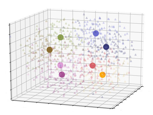
(a) 3D plot of three-level hierarchy (8 clusters)

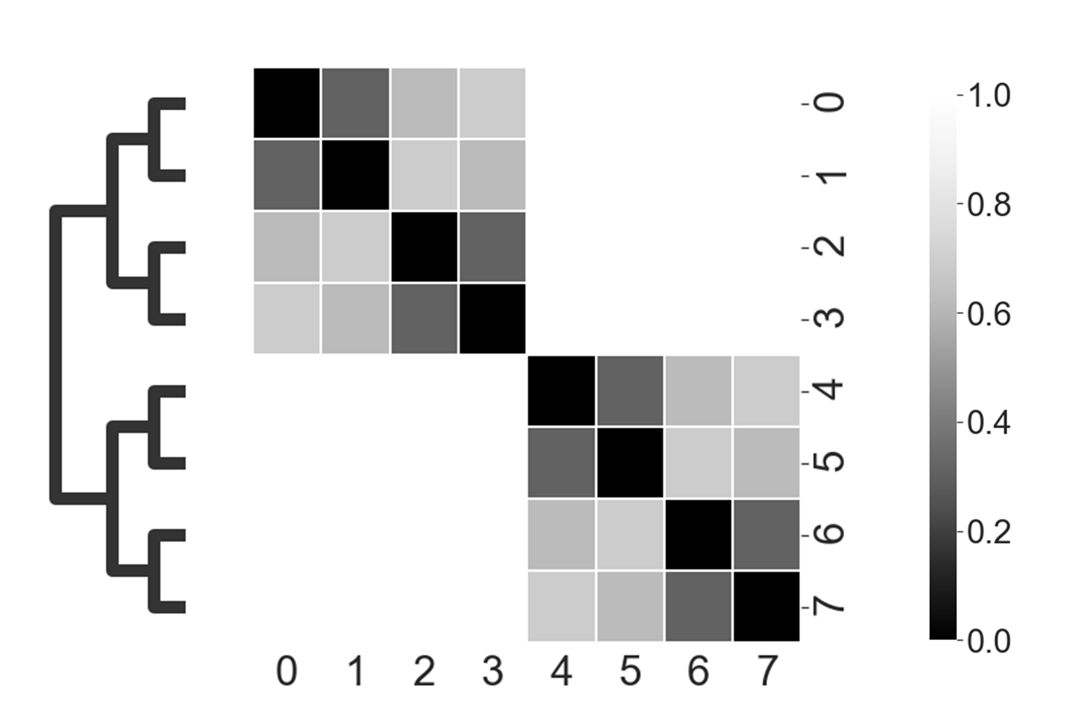
(b) Ground truth dendrogram & distance matrix

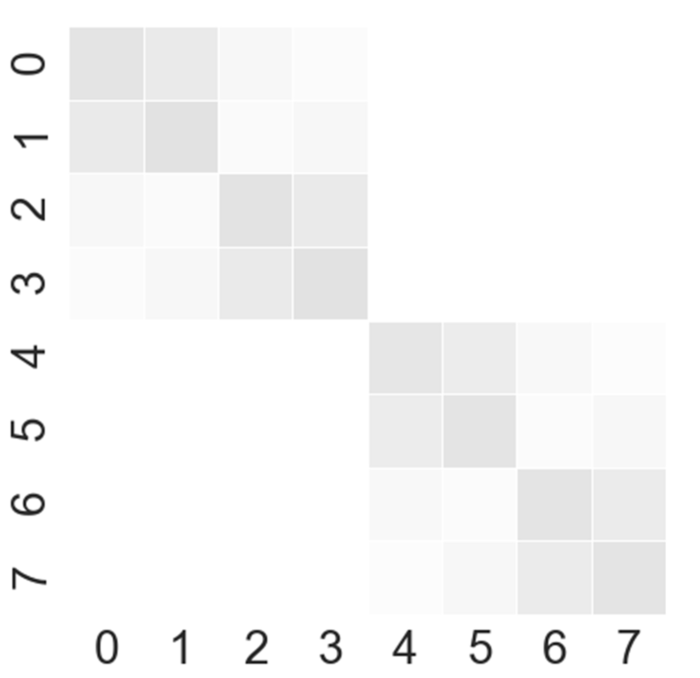
(c) Dataset with shifted means

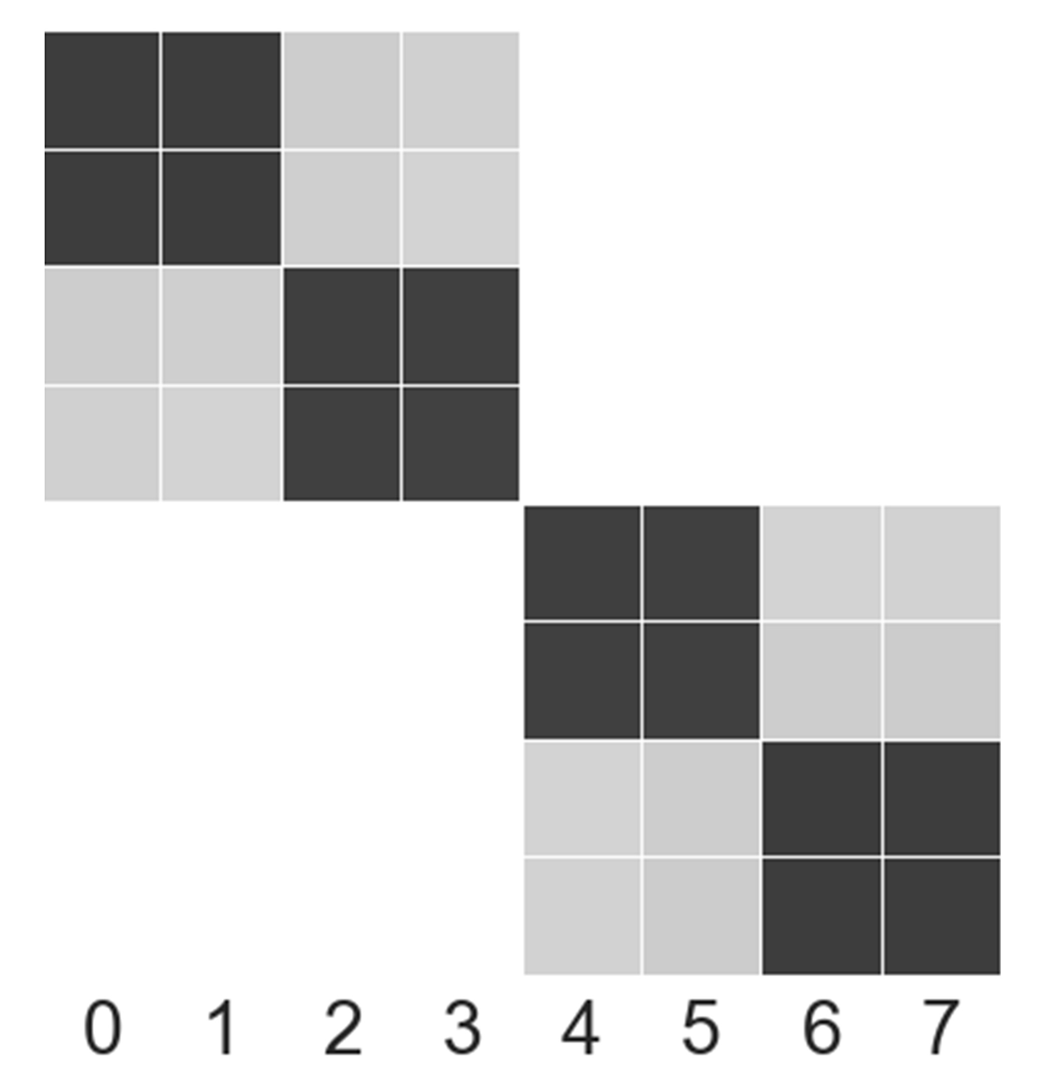
(d) PCA on shifted dataset

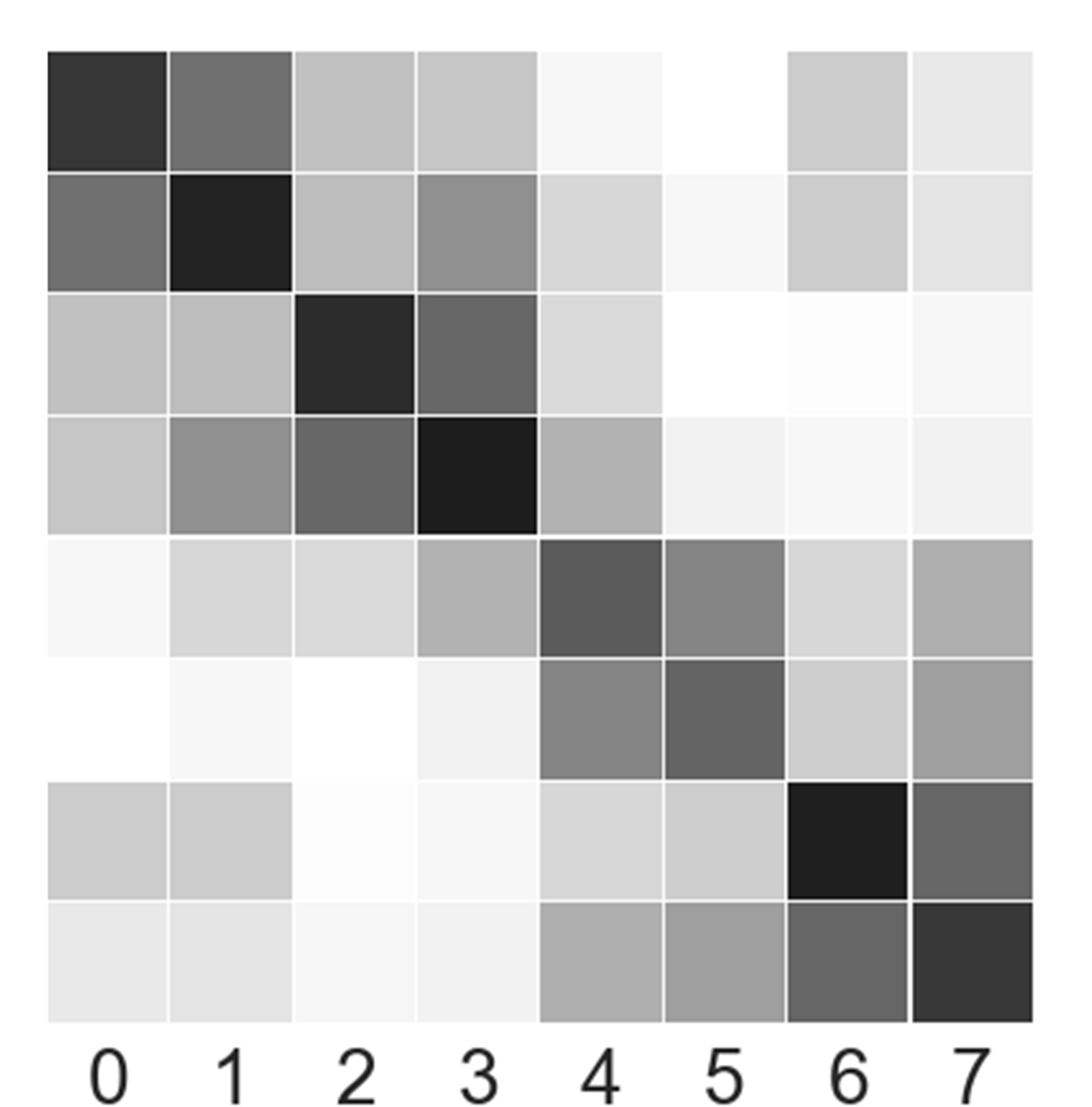
(e) VaDE on shifted dataset

Figure 1: Top row: Synthetic data demonstrating a three-level hierarchy encoded via the pairwise Euclidean distances between eight clusters. Bottom row: Effect of shifting half of the means by cyclically rotating the vectors, e.g., $(4,2,1,0,0,0)\mapsto(0,0,0,4,2,1)$. Comparing PCA and VaDE shows that a non-linear embedding can increase cluster separation and roughly preserve the hierarchy.

2 Clustering Models and Objectives

Planted Hierarchies with Noise.   We introduce a simple heuristic of constructing a mixture of Gaussians that also encodes hierarchical structure via Euclidean distances. In particular, the resulting new construction (i) approximately models the latent space of VaDE, and (ii) allows us to test the effectiveness of VaDE in increasing the separation among clusters.

We shall refer to our model as BTGM, Binary Tree Gaussian Mixture, formed by a uniform mixture of spherical Gaussians with shared variance and different means. The model is determined by four parameters: height $h$, margin $m$, and dimension $d$, and expansion ratio $\alpha$, a constant satisfying $\alpha>1$. Specifically, in a BTGM with height $h$ and margin $m$, we construct $2^{h}$ spherical Gaussian distributions with unit variance $I_{d}$ and mean vectors $\mu_{i}\in\mathbb{R}^{d}$, whose $j^{th}$ coordinate $\mu_{i}[j]$ is specified by the following equation.

$$\mu_{i}[j]=\begin{cases}(-1)^{p_{i,j}}\cdot m\cdot\alpha^{h-j},\textrm{ for }\\ \hskip 20.00003ptp_{i,j}\equiv i\!\!\!\!\pmod{2^{h-i}}\textrm{ and }j\leq h\\ 0,\ \textrm{if }h<j\leq d.\end{cases}$$ (1)

At a high level, we constructed a complete binary tree of height $h$, with each leaf corresponding to a spherical Gaussian distribution. A crucial structural property is that the distance between any two means, $\mu_{i}$ and $\mu_{j}$, is positively related to their distance in the binary tree. More precisely,

$$\left\lVert\mu_{i}-\mu_{j}\right\rVert_{2}\geq m\cdot\alpha^{\mathsf{ht}(\mathsf{LCA}(\mu_{i},\mu_{j}))},$$

where $\mathsf{ht}(v)$ denotes the height of node $v$ in the tree, and $\mathsf{LCA}$ is the least common ancestor of two nodes. Figure 1 depicts an instance of the BTGM model with parameters $m=4$, $h=3$, $\alpha=2$, and $d=100$. Figure 1(a) presents the 3D tSNE visualization of the data, and Figure 1(b) shows the pairwise distance matrix (normalized to $[0,1]$) of the clusters and the ground-truth hierarchy. We also define a non-linear shifting operation on the BTGM, which increases the difficultly of recovering the structure and allows more flexibility in experiments. Specifically, we shift the nonzero mean-vector entries of the first $\frac{k}{2}$ BTGM components to arbitrary new locations, e.g., we may shift $\mu_{1}$ from $(4,2,1,0,0,0)$ to $(0,0,0,4,2,1)$ via rotation in a BTGM with $k=8,h=3$, $\alpha=2$, and $m=2$. After the operation, the model’s hierarchical structure is less clear from the mean distances in the $h$-dimensional Euclidean subspace. Other non-linear operations can be applied to model different data types.

Data Separability.   Our synthetic model and our theoretical results assume that the dataset satisfies certain separability requirements. Such properties do not hold for real datasets before applying the embedding. Fortunately, the assumptions are not about the original data, but about the transformed dataset. We observe that VaDE increases the separation between different clusters, and we also see that it preserves some of the hierarchical information as well. Therefore, in the rest of the paper, we consider separation assumptions that are justified by the fact that we apply a learned embedding to the dataset before running any clustering algorithm. For more details, see Figure 8 in Appendix C, which shows the separation on MNIST.

2.1 Hierarchical Clustering Objectives

Index the dataset as $\mathcal{X}=\{x_{1},\ldots,x_{n}\}$. Let $\mathsf{leaves}(\mathsf{T}[i\vee j])\subseteq\mathcal{X}$ denote the set of leaves of the subtree in $\mathsf{T}$ rooted at $\mathsf{LCA}(x_{i},x_{j})$, the least common ancestor of $x_{i}$ and $x_{j}$. Given pairwise similarities $w_{ij}$ between $x_{i}$ and $x_{j}$, Dasgupta’s cost dasgupta2016cost minimizes $\mathsf{cost}(\mathsf{T})=\sum_{i,j\in[n]}w_{ij}\cdot|\mathsf{leaves}(\mathsf{T}[i\vee j])|.$ Moseley-Wang’s objective MoseleyWang is a dual formulation, based on maximizing

$$\mathsf{MW}(\mathsf{T})=n\sum_{i,j\in[n]}w_{ij}-\mathsf{cost}(\mathsf{T}).$$ (2)

Dendrogram purity heller2005bayesian uses ground truth clusters $\mathcal{C}=\{C^{*}_{1},\ldots,C^{*}_{k}\}$. Let $\mathcal{P}^{*}$ be the set of pairs in the same cluster: $\mathcal{P}^{*}=\{(x^{i},x^{j})\mid\mathcal{C}(x^{i})=\mathcal{C}(x^{j})\}$. Then,

$$\mathsf{DP}(\mathsf{T})\!=\frac{1}{|\mathcal{P}^{*}|}\sum_{\ell=1}^{k}\sum_{x^{i},x^{j}\in C^{*}_{\ell}}\!\!\mathsf{pur}(\mathsf{leaves}(\mathsf{T}[i\vee j]),C^{*}_{\ell}),$$ (3)

where $\mathsf{pur}(A,B)=|A\cap B|/|A|.$

Ward’s Method.   Let $C_{1},\ldots,C_{k}$ be a $k$-clustering. Let $\mu(C)=\frac{1}{|C|}\sum_{x\in C}x$ denote the mean of cluster $C$. Ward’s method ward1963hierarchical ; grosswendt2019analysis merges two clusters to minimize the increase in sum of squared distances:

$$\min_{i,j}\sum_{x\in C_{i}\cup C_{j}}\|x-\mu(C_{i}\cup C_{j})\|_{2}^{2}-\sum_{x\in C_{i}}\|x-\mu(C_{i})\|_{2}^{2}-\sum_{x\in C_{j}}\|x-\mu(C_{j})\|_{2}^{2}.$$

3 Embedding with VaDE

VaDE jiang2017variational considers the following generative model specified by $p(x,z,c)=p(x\mid z)p(z\mid c)p(c)$. We use $\mathsf{Cat}(.)$ to denote a categorical distribution, $\mathcal{N}(.)$ is a normal distribution, and $k$ is the predefined number of clusters. In the following, $\mu_{c}$ and $\sigma^{2}_{c}$ are parameters for the latent distribution, and $\hat{\mu}_{z}$ and $\hat{\sigma}^{2}_{z}$ are outputs of $f(z;\theta)$, parametrized by a neural network. And the generative process for the observed data is

$$c\sim\mathsf{Cat}(1/k),\ z\sim\mathcal{N}(\mu_{c},\sigma^{2}_{c}\cdot I),\ x\sim\mathcal{N}(\hat{\mu}_{z},\hat{\sigma}^{2}_{z}\cdot I).$$ (4)

The VaDE maximizes the likelihood of the data, which is bounded by the evidence lower bound,

$$\begin{split}L_{\text{\tiny ELBO}}&=E_{q(z,c|x)}[\log p(x\!\mid\!c)]\\ &\hskip 50.00008pt-D_{\text{KL}}(q(z,c\!\mid\!x)\ \|\ p(z,c)),\end{split}$$ (5)

where $q(z,c\mid x)$ is a variational posterior to approximate the true posterior $p(z,c\mid x)$. We use a neural network $g(x;\phi)$ to parametrize the model $q(z\mid x)$. We refer to the original paper for the derivation of Eq. (5) and for the connection of $L_{\text{ELBO}}$ to the gradient formulation of the objective jiang2017variational .

3.1 Improving separation by rescaling means

The VaDE landscape is a mixture of multiple Gaussian distributions. As we will see in Section 4, the separation of Gaussian distributions is crucial for Ward’s method to recover the underlying clusters. Since Ward’s method is a local heuristic, data points that lie in the middle area of two Gaussians are likely to form a larger cluster before merging into one of the true clusters. This “problematic” cluster will further degrade the purity of the dendrogram. However, the objective that VaDE optimizes does not encourage a larger separation. As a result, we apply a transformation to the VaDE latent space to enlarge the separation between each Gaussians. Let $x^{\prime}_{i}$ be the embedded value of the data point $x_{i}$, and define

$$\mathcal{C}(x^{\prime}_{i})=\mathrm{argmax}_{j}[p(x^{\prime}_{i}\mid\mu_{c=j},\ \sigma^{2}_{c=j}\cdot I)]$$

to be the cluster label assigned by the learned GMM model. Then, we compute the transformation

$$x^{\prime\prime}_{i}=x^{\prime}_{i}+s\cdot\mu_{i}\text{ with }\mu_{i}=\mu_{c=\mathcal{C}(x_{i})},$$

where $s$ is a positive rescaling factor. The transformation has the following properties: (i) for points assigned to the same Gaussian by the VaDE method, the transformation preserves their pairwise distances; (ii) if $x_{i}$’s assigned to the same $\mu$ by $\mathcal{C}$ are i.i.d. random variables with expectation $\mu$ (which coincides with the intuition behind VaDE), then the transformation preserves the ratio between the distances of the expected point locations associated with different mean values.

Appendix C illustrates how to choose $s$ in detail. To improve both DP and MW, the rule of thumb is to choose a scaling factor $s$ large enough. We set $s=3$ for all datasets. In summary, we propose the following hierarchical clustering procedure:

1. Train VaDE on the unlabeled dataset $\{x_{1},\ldots,x_{n}\}$.

2. Embed $x_{i}$ using the value mapping $x_{i}^{\prime}=\hat{\mu}_{\hat{z}}$ where $(\hat{\mu}_{\hat{z}},\log\hat{\sigma}_{\hat{z}}^{2})=f(\hat{z};\ \theta)$ and $\hat{z}=g(x_{i}\ ;\ \phi)$.

3. Choose a rescaling factor $s$ and apply the rescaling transformation on each $x^{\prime}_{i}$ to get $x^{\prime\prime}_{i}$.

4. Run Ward’s method on $\{x^{\prime\prime}_{i}\}_{i=1}^{n}$ to produce a hierarchical clustering.

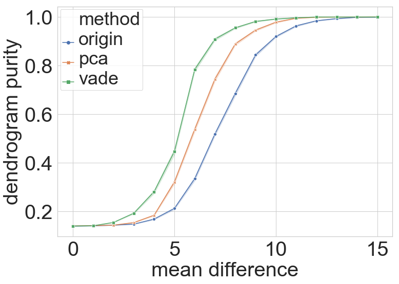
(a) Dendrogram Purity

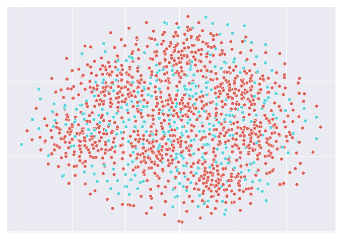
(b) Original + Ward

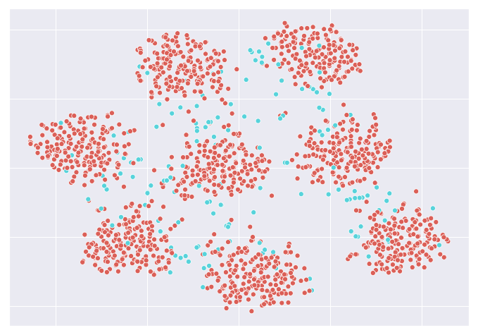
(c) PCA + Ward

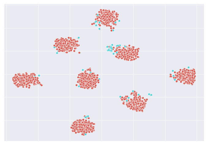
(d) VaDE + Ward

Figure 2: (a) DP of Ward’s method on original, PCA, and VaDE space, varying mean separation. (b)(c)(d) show 8 clusters recovered by running Ward’s method on original, PCA and VaDE latent space (Ward’s method terminates when there are 8 clusters). Data drawn from 8 spherical Gaussians in $\mathbb{R}^{100}$ with pairwise mean separation 8. Point clouds generated by tSNE; Red colors indicate correct cluster labels assigned by Ward’s method, and blue indicates wrong cluster.

4 Theoretical Analysis

We provide theoretical guarantees for Ward’s method on separated data, providing justification for using VaDE (proofs in Appendix A). Here, we focus on the mixture model of spherical Gaussians. We are given a sample of size $n$, say $X_{1},\ldots,X_{n}$, where each point $X_{i}\in\mathbb{R}^{d}$ is independently drawn from one of $k$ Gaussian components according to mixing weights $w_{1},\ldots,w_{k}$, with the $j$-th component having mean $\mu_{j}\in\mathbb{R}^{d}$ and covariance matrix $\Sigma_{j}\in\mathbb{R}^{d\times d}$. Specifically, for any component index $j$, we assume that the covariance $\Sigma_{j}$ satisfies $\Sigma_{j}=\sigma_{j}^{2}\cdot I_{d}$, where $\sigma_{j}>0$ and $I_{d}\in\mathbb{R}^{d\times d}$ is the identity matrix. Under this assumption, the model is fully determined by the set of parameters $\{(w_{i},\mu_{i},\sigma_{i}):\forall i\in[k]\}$. The goal is to cluster the sample points by their associated components.

The theorem below presents sufficient conditions for Ward’s method to recover the underlying $k$-component clustering when points are drawn from a $k$-mixture of spherical Gaussians. To recover a $k$-clustering, we terminate when there are $k$ clusters.

Theorem 1.

Let $c,c_{0}>0$ be absolute constants. Suppose we have $n$ samples from a $k$-mixture of spherical Gaussians with parameters $\{(w_{i},\mu_{i},\sigma_{i}):w_{i}>0,\forall i\in[k]\}$ satisfying

$$\forall i\not=j\in[k],\left\lVert\mu_{i}-\mu_{j}\right\rVert_{2}\geq c\sqrt{\nu}(\sigma_{i}+\sigma_{j})(\sqrt{d}+\sqrt{\log n}),$$

where $\nu:=\max_{\ell\not=t}w_{\ell}/w_{t}$, and suppose $n\geq\frac{c_{0}}{w_{\text{\tiny min}}}\log k$, where $w_{\text{\tiny min}}\!:=\!\min_{t}w_{t}$. Ward’s method will recover the underlying $k$-clustering with probability at least $1-2/k$.

As a recap, Ward’s method starts with singleton clusters, and repeatedly selects a pair of clusters and merges them into a new cluster, where the selection is based on the optimal value of the error sum of squares. In particular, recovering the underlying $k$-component clustering means that every cluster contains only points from the same Gaussian component when the algorithm produces a $k$-clustering.

4.1 Intuition and Optimality

On a high level, the mean separation conditions in Theorem 1 guarantee that with high probability, the radiuses of the clusters will be larger than the inter-cluster distances, and the sample lower bound ensures that we observe at least constant many sample points from every Gaussian, with high probability. In Appendix B, we illustrate the hardness of improving the theorem without pre-processing the data, e.g., applying an embedding method to the sample points, such as VaDE or PCA. In particular, we show that (i) without further complicating the algorithm, the separation conditions in Theorem 1 have the right dependence on $d$ and $n$; (ii) for exact recovery, the sample-size lower bound in Theorem 1 is also tight up to logarithmic factors of $k$.

These results and arguments indeed justify our motivation for combining VaDE with Ward’s method. To further demonstrate our approach’s power, we experimentally evaluate the clustering performance of three methods on high-dimensional equally separated Gaussian mixtures – the vanilla Ward’s method, the PCA-Ward combination, and the VaDE-Ward combination. As shown in Figure 2(a), in terms of the dendrogram purity, Ward’s method with VaDE pre-processing tops the other two, for nearly every mean-separation level. In terms of the final clustering result in the (projected) space, Figures 2(b) to 2(d) clearly shows the advantage of the VaDE-Ward method as it significantly enlarges the separation among different clusters while making much fewer mistakes in the clustering accuracy.

Next, we show that given the exact recovery in Theorem 1 and mild cluster separation conditions, Ward’s method recovers the exact underlying hierarchy.

For any index set $I\subseteq[k]$ and corresponding Gaussian components $\mathcal{G}_{i},i\in I$, denote by $w_{I}$ the total weight $\sum_{i\in I}w_{i}$, and by $C_{I}$ the union of sample points from these components. We say that a collection $\mathcal{H}$ of nonempty subsets of $[k]$ form a hierarchy of order $\tau$ over $[k]$ if there exists a index set sequence $T_{\ell}$ for $\ell=1,\ldots,\tau$ such that i) for every $\ell$, the set $\mathcal{H}_{\ell}$ partitions $[k]$; ii) $\mathcal{H}_{k}$ is the union of $\mathcal{H}_{\ell}:=\{I_{\ell t}:t\in T_{\ell}\}$; iii) for every $\ell<\tau$ and $t\in T_{\ell}$, we have $I_{\ell t}\subseteq I_{(\ell+1)t^{\prime}}$ for some $t^{\prime}\in T_{\ell+1}$.

For any sample size $n$ and Gaussian component $\mathcal{G}_{i}$, denote by $S_{i}:=\sigma_{i}(\sqrt{d}+2\sqrt{\log n})$, which upper bounds the radius of the corresponding sample cluster, with high probability. The triangle inequality then implies that for any $i\not=j\in[k]$, the distance between a point in the sample cluster of $\mathcal{G}_{i}$ and that of $\mathcal{G}_{j}$ is at most $D_{ij}^{+}:=\left\lVert\mu_{i}-\mu_{j}\right\rVert_{2}+S_{i}+S_{j}$, and at least $D_{ij}^{-}:=\left\lVert\mu_{i}-\mu_{j}\right\rVert_{2}-S_{i}-S_{j}$. Naturally, we also define $D_{I,J}^{+}:=\max_{i\in I,j\in J}D_{ij}^{+}$ and $D_{I,J}^{-}:=\min_{i\in I,j\in J}D_{ij}^{-}$ for any $I,J\subseteq[k]$, serving as upper and lower bounds on the cluster-level inter-point distances. These compact notations give our theoretical claim a simple form.

Theorem 2.

There exists an absolute constant $c_{1}<8$ such that the following holds. Suppose we have $n$ samples from a $k$-mixture of spherical Gaussians that satisfy the conditions and sample size bound in Theorem 1, and suppose there is an underlying hierarchy of the Gaussian components $\mathcal{H}$ satisfying

$$\forall\ell\in[s],\ \ I\not=J\in\mathcal{H}_{\ell},\ \ D_{I,J}^{-}\geq c_{1}\sqrt{\nu_{\ell}}\max\{D_{I,I}^{+},D_{J,J}^{+}\},$$

where $\nu_{\ell}:=\max_{I\not=J\in\mathcal{H}_{\ell}}w_{I}/w_{J}$. Then, Ward’s method recovers the underlying hierarchy $\mathcal{H}$ with probability at least $1-2/k$.

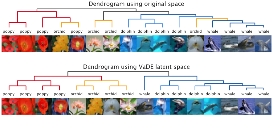
Figure 3: In the original space, Ward’s method makes several mistakes: three orchids merge into the aquatic animals cluster before the flowers cluster. Using the VaDE embedding, Ward’s method produces a near optimal dendrogram on this subset of data for both lower and higher level structures.

Table 1: Dendrogram Purity and Moseley-Wang’s objective on BTGM synthetic dataset with $\alpha=2$. We evaluate Ward’s method using different embeddings, while varying parameters: $k$ denotes the number of pure clusters, $h$ denotes both the dimension of the PCA and VaDE latent spaces and the tree height.

	$k$ = 8 ($h$ = 3)	$k$ = 16 ($h$ = 4)	$k$ = 32 ($h$ = 5)
Original	0.798 $\pm$ .020	0.789 $\pm$ .017	0.775 $\pm$ .016
PCA	0.518 $\pm$ .002	0.404 $\pm$ .003	0.299 $\pm$ .003
VAE	0.619 $\pm$ .030	0.755 $\pm$ .019	0.667 $\pm$ .012
VaDE	0.943 $\pm$ .011	0.945 $\pm$ .001	0.869 $\pm$ .013

(a)

$k=8\ (h=3)$	$k=16\ (h=4)$	$k=32\ (h=5)$
0.960 $\pm$ 0.004	0.980 $\pm$ 0.002	0.989 $\pm$ 0.001
0.909 $\pm$ 0.001	0.913 $\pm$ 0.004	0.936 $\pm$ 0.001
0.791 $\pm$ 0.028	0.898 $\pm$ 0.017	0.969 $\pm$ 0.011
0.990 $\pm$ 0.020	0.994 $\pm$ 0.001	0.991 $\pm$ 0.001

(b)

Table 2: DP on four real datasets for different embedding methods.

	Reuters	MNIST	CIFAR-25	20 Newsgroups
Original	0.535	0.478	0.110	0.225
PCA	0.587	0.472	0.108	0.203
VAE	0.468	0.495	0.082	0.196
VaDE	0.650	0.803	0.120	0.248
VaDE + Trans.	0.672	0.886	0.128	0.251

Table 3: MW (ratio vs. opt) on four real datasets for different embedding methods.

	Reuters	MNIST	CIFAR-25	20 Newsgroups
Original	0.654	0.663	0.423	0.557
PCA	0.679	0.650	0.435	0.575
VAE	0.613	0.630	0.393	0.548
VaDE	0.745	0.915	0.455	0.595
VaDE + Trans.	0.768	0.955	0.472	0.605

The above theorem resembles Theorem 1, with separation conditions comparing the cluster radiuses with the inter-cluster distances at different hierarchy levels. Informally, the theorem states that if the clusters in each level of the hierarchy are well-separated, Ward’s method will be able to recover the correct clustering of that level, and hence also the entire hierarchy.

Recall from Section 2 that a BTGM, Binary Tree Gaussian Mixture, is a mixture of Gaussians that encode the hierarchy. For the BTGM in Eq. (1), the shared variance implies that $S:=S_{i}=\sqrt{d}+2\sqrt{\log n}$ is a constant for any $i\in[k]$, yielding $D_{I,I}^{+}=\max_{i,j\in I}\left\lVert\mu_{i}-\mu_{j}\right\rVert_{2}+2S$ for any $I\subseteq[k]$. Then by symmetry, we see that $\nu_{\ell}=1$, $\max_{i,j\in I}\left\lVert\mu_{i}-\mu_{j}\right\rVert_{2}+2S$, and $D_{I,J}^{-}+2S\geq\alpha(D_{I,I}^{+}-2S)\geq\alpha m$ for any level $\ell$ and $I\not=J\in\mathcal{H}_{\ell}$. Consolidating Theorem 1 and 2 with these simplifications yields the following result.

Corollary 1.

Consider the BTGM in Equation 1 and let $k:=2^{h}$ be the component number. Let $c,c_{0}$, and $c_{1}$ be the absolute constants in Theorem 1 and 2, and define a constant $c_{2}:=2(2c_{1}+1)/(\alpha-c_{1})$. If the sample size satisfies $n\geq c_{0}\cdot k\log k$ and the model is well-separated with $\alpha>c_{1}$ and $m\geq 2\max\{c,c_{2}\}\cdot(\sqrt{d}+\sqrt{\log n})$, then Ward’s method recovers the underlying hierarchy $\mathcal{H}$ with probability at least $1-2/k$.

5 Experiments

Our main experimental goal is to determine which embedding method produces the best results for dendrogram purity and Moseley-Wang’s objective. In this section, we focus on Ward’s method for clustering after embedding (Appendix C has other algorithms).

Set-up and methods.   We compare VaDE against PCA (linear baseline) and a standard VAE (non-linear baseline). We run Ward’s method on the embedded or original data to get dendrograms. We test on four real datasets: Reuters and MNIST with flat clustering labels (i.e., 1-level hierarchy); 20 Newsgroups (3-level hierarchy) and CIFAR-25 (2-level hierarchy). We only use 25 classes from CIFAR-100 that fall into one of the five superclasses “aquatic animals”, “flowers”, “fruits and vegetables”, “large natural outdoor scenes” and “vehicle1”. We call it CIFAR-25. For 20 Newsgroups and CIFAR-25, we use the full dataset, but for MNSIT and Reuters, we average results over 100 runs, each with 10,000 random samples. Embedding methods are trained on the whole dataset. Details in Appendix C. We set the margin $m$ of the BTGM to be 8 while varying the depth, so the closest distance between the means of any two Gaussian distributions is 8.

Synthetic Data (BTGM).   We vary the depth and margin of BTGM to evaluation various hierarchy depths and cluster separations. After generating $k$ means for the BTGM, we shift all non-zero entries of the first $\frac{k}{2}$ means to an arbitrary location. We show that this simple non-linear transformation is challenging for linear embedding methods (i.e., PCA), even though it preserves hierarchical structure. To generate $k$ clusters with shifted means, we sample 2000 points from each Gaussian distribution of the BTGM of height $h$ such that $2^{h}=k$ for $h=3,4,5$. Then, $h$ is the embedding dimension of PCA, VAE, and VaDE.

Dendrogram Purity (DP).   We compute the DP of various methods using Eq. (3). We construct ground truth clusters either from class labels of real datasets or from the leaf clusters of the BTGM model.

Moseley-Wang’s Objective (MW).   To evaluate the MW objective in Eq. (2), we need pairwise similarities $w_{ij}$. We define the similarities based on the ground truth labels and hierarchy. Let $h$ denote the depth of the hierarchy (which ranges between 1 and 5 in our experiments). We use $w_{ij}=2^{l-1}\cdot\mathbbm{1}_{\mathcal{C}^{l}(x^{i})=\mathcal{C}^{l}(x^{j})}$, $l\in[h]$, where $\mathcal{C}^{l}(x^{i})$ denotes the label for point $x^{i}$ at the $l^{th}$ level of the hierarchical tree from top to bottom. We report the ratio achieved by various methods to the optimal MW value opt that we compute as follows. When there are hierarchical labels, we compare against the optimal tree with ground truth levels. Otherwise, for flat clusters, opt is obtained by merging points in the same clusters, then building a binary tree on top.

5.1 Results

Results on Synthetic Data.   Table 3(b) presents the results of the synthetic experiments. Embedding with VaDE and then clustering with Ward’s method leads to the best DP and MW results in all settings. For DP, we see that PCA performs the worst, while the original (non-embedded) data has the second-best results, and the difference between the results is larger than the empirical standard deviation. For MW, the results are more similar to each other, and perhaps surprisingly, the relative performance changes with the depth. The latent distributions learned by VaDE are already well-separated, so the rescaling is not necessary in this case.

Results on Real Data.   Tables 2 and 3 report DP and MW objectives on real datasets. We observe that for MNIST, using the VaDE embedding improves DP and MW significantly compared to other embeddings, and applying the transformation further leads to an increased value of both objectives. The results on the Reuters and 20 Newsgroups datasets show that VaDE plus the rescaling transformation is also suitable for text data, where it leads to the best performance. In the CIFAR-25 experiments, we see only a modest improvement with VaDE when evaluating with all 25 classes. We also observe from the table that these two objectives are positively correlated for most of the cases. The only exception occurs when we apply PCA to CIFAR-25 and 20 Newsgroups. PCA embedding increases the MW objective but decreases the DP comparing to the original data. Note that we utilize the hierarchical labels while computing the MW objective for CIFAR-25 and 20 Newsgroups. One possible reason is that PCA can only separate super-clusters in the higher level, but it fails to separate clusters in the lower level of the hierarchical tree. Therefore it results in worse DP but better MW performance.

5.2 Discussion

In Theorems 1 and 2, and Corollary 1, we studied the performance of Ward’s method on the fundamental Gaussian mixture model. We showed that with high probability, Ward’s method perfectly recovers the underlying hierarchy under mild and near-optimal separability assumptions in Euclidean distance. Since VaDE uses a GMM prior, this is a natural metric for the embedded space. As the rescaling increases the separation, we suppose that the embedded vectors behave as if they are approximately sampled from a distribution satisfying the conditions of the theorems. Consequently, our theoretical results justify the success of the embedding in practice, where we see that VaDE+Transformation performs the best on many datasets. We hypothesize that VaDE generates a latent space that encodes more of the high level structure for the CIFAR-25 images. This hypothesis can be partially verified by the qualitative evaluation in Figure 3. A trend consistent with the synthetic experiments is that PCA and VAE are not always helpful embeddings for hierarchical clustering with Ward’s method. Overall, VaDE discovers an appropriate embedding into Euclidean space based on its GMM prior that improves the clustering results.

The synthetic results in Table 3(b) exhibit the success of the VaDE+Transformation method to recover the underlying clusters and the planted hierarchy. This trend holds while varying the number of clusters and depth of the hierarchy. Qualitatively, we find that VaDE can “denoise” the sampled points when the margin does not suffice to guarantee non-overlapping clusters. This enables Ward’s method to achieve a higher value of DP and MW than running the algorithm on the original data. In many cases, embedding with PCA or VAE is actually detrimental to the two objectives compared to the original data. We conjecture that the difference in performance arises because VaDE fully utilizes the $h$-dimensional latent space, but PCA fails to resolve the non-linear shifting of the underlying means. In general, using a linear embedding method will likely lead to a drop in both DP and MW for this distribution. Similarly, VAE does not provide sufficient separation between clusters. The BTGM experiments showed (i) the necessity of using non-linear embedding methods and (ii) VaDE’s ability to increase the separation between clusters.

The rescaling transformation leads to consistently better results for both DP and MW on multiple real datasets. In practice, the data distributions are correlated and overlapping, without clear cluster structure in high-dimensional space. The VaDE embedding leads to more concentrated clusters, and the rescaling transformation enlarges the separation enough for Ward’s method to recover what is learned by VaDE.

6 Conclusion

We investigated the effectiveness of embedding data in Euclidean space to improve unsupervised hierarchical clustering methods. Motivated by unsupervised tasks such as taxonomy construction and phylogeny reconstruction, we studied the improvement gained by combining embedding methods with linkage-based clustering algorithms. We saw that rescaling the VaDE latent space embedding, and then applying Ward’s linkage-based method, leads to the best results for dendrogram purity and the Moseley-Wang objective on many datasets. To better understand the VaDE embedding, we proposed a planted hierarchical model using Gaussians with separated means. We proved that Ward’s method recovers both the clustering and the hierarchy with high probability in this model. Compared to methods that use hyperbolic embeddings gu2018learning ; mathieu2019continuous ; nickel2017poincare or ultrametrics chierchia2019ultrametric , we believe that our approach will be easier to integrate into existing systems.

While we focus on embedding using variational autoencoders, an open direction for could involve embedding hierarchical structure using other representation learning methods agarwal2007generalized ; borg2005modern ; caron2018deep ; chierchia2019ultrametric ; mishne2019diffusion ; nina2019decoder ; salakhutdinov2012one ; tsai2017learning ; yadav2019supervised . Another direction is to better understand the similarities and differences between learned embeddings, comparison-based methods, and ordinal relations emamjomeh2018adaptive ; ghoshdastidar2019foundations ; jamieson2011low ; kazemi2018comparison . Finally, a large number of clusters may be a limitation of the VaDE embedding, and this deserves attention.

Appendix A Proof of the Theorems

The next two lemmas provide tight tail bounds for binomial distributions and spherical Gaussians.

Lemma 1 (Concentration of binomial random variables).

[16] Let $X$ be a binomial random variable with mean $\mu$, then for any $\delta>0$,

$$\Pr(X\geq{(1+\delta)\mu})\leq{e^{-(\max\{\delta^{2},\delta\})\mu/3}},$$

and for any $\delta\in{(0,1)}$,

$$\Pr(X\leq{(1-\delta)\mu})\leq{e^{-\delta^{2}\mu/2}}.$$

Lemma 2 (Concentration of spherical Gaussians).

[36] For a random $X$ distributed according to a spherical Gaussian in $d$ dimensions (mean $\mu$ and variance $\sigma^{2}$ in each direction), and any $\delta\in(0,1)$,

$$\Pr\left(\left\lVert X-\mu\right\rVert_{2}^{2}\leq\sigma^{2}d\left(1+2\sqrt{\frac{\log(1/\delta)}{d}}+\frac{2\log(1/\delta)}{d}\right)\right)\geq 1-\delta.$$

Lemma 3 (Optimal clustering through Ward’s method).

[31, 32] Let $P\subseteq\mathbb{R}^{d}$ be a collection of points with underlying clustering $C_{1}^{*},\ldots,C_{k}^{*}$, such that the corresponding cluster mean values $\mu_{1}^{*},\ldots,\mu_{k}^{*}$ satisfy $\left\lVert\mu_{i}^{*}-\mu_{j}^{*}\right\rVert_{2}>(2+2\sqrt{2\nu})\max_{x\in C_{i}^{*}}\left\lVert x-\mu_{i}^{*}\right\rVert_{2}$ for all $i\not=j$, where $\nu:=\max_{\ell,t\in[k]}\frac{|C_{\ell}^{*}|}{|C_{t}^{*}|}$ is the maximum ratio between cluster sizes. Then Ward’s method recovers the underlying clustering.

Now we are ready to prove Theorem 1 1.

Proof of Theorem 1.

First, for each component in the mixture, we determine the associated number of sample points. This is equivalent to drawing a size-$n$ sample from the weighting distribution that assigns $w_{i}>0$ to each $i\in[k]$. The number of times each symbol $i\in[k]$ appearing in the sample, which we refer to as the (sample) multiplicity of the symbol, follows a binomial distribution with mean $nw_{i}$. By Lemma 1, the probability that an arbitrary multiplicity is within a factor of $2$ from its mean value is at least $1-2e^{-nw_{i}/8}$. Hence, for $n\geq 16(\log k)/w_{i}$, the union bound yields that this deviation bound holds for all symbols with probability at least $1-k\cdot k^{-2}=1-k^{-1}$.

Second, given the symbol multiplicities, we draw sample points from each component correspondingly. Consider the $i$-th component with mean $\mu_{i}$. Then, by Lemma 2, every sample point from this component deviates (under Euclidean distance) from $\mu_{i}$ by at most $S_{i}:=\sigma_{i}(\sqrt{d}+2\sqrt{\log n})$, with probability at least $1-n^{-2}$. Again, the union bound yields that this deviation bound holds for all components and all sample points with probability at least $1-n\cdot n^{-2}=1-n^{-1}$.

Third, by the above reasoning and $n>k$, with probability at least $1-2/k$ and for all $i\in[k]$,

1. the sample size associated with the $i$-th component is between $nw_{i}/2$ and $2nw_{i}$;

2. every sample point from the $i$-th component deviates from $\mu_{i}$ by at most $S_{i}$.

Therefore, if further $\left\lVert\mu_{i}-\mu_{j}\right\rVert_{2}\geq(5+12\max_{\ell,t\in[k]}\sqrt{w_{\ell}/w_{t}})(S_{i}+S_{j})$ for all $i\not=j$, the sample points will form well-separated clusters according to the underlying components. In addition, the first assumption ensures that the maximum ratio between cluster sizes is at most $4\max_{\ell,t\in[k]}\sqrt{w_{\ell}/w_{t}}$, and the second assumption implies that for any $i\not=j\in[k]$,

1. the $i$-th cluster the distance between the mean to any point in it is at most $2S_{i}$;

2. the empirical means of the $i$-th and $j$-th clusters are separated by at least

   $$16(S_{i}+S_{j})>\left(2+2\sqrt{2\cdot 4}\cdot\max_{\ell,t\in[k]}\sqrt{\frac{w_{\ell}}{w_{t}}}\right)\max\{2S_{i},2S_{j}\}.$$

Finally, applying Lemma 3 completes the proof of the theorem. ∎

Next, we move to the proof of Theorem 2. Let us first recap what the theorem states.

Theorem 2.

There exists an absolute constant $c_{1}>0$ such that the following holds. Suppose we are given a sample of size $n$ from a $k$-mixture of spherical Gaussians that satisfy the separation conditions and the sample size lower bound in Theorem 1, and suppose that there is an underlying hierarchy of the Gaussian components $\mathcal{H}$ satisfying

$$\forall\ell\in[s],\quad I\not=J\in\mathcal{H}_{\ell},\quad D_{I,J}^{-}\geq c_{1}\sqrt{\nu_{\ell}}\ (D_{I,I}^{+}+D_{J,J}^{+}),$$

where $\nu_{\ell}:=\max_{I\not=J\in\mathcal{H}_{\ell}}w_{I}/w_{J}$. Then, Ward’s method recovers the underlying hierarchy $\mathcal{H}$ with probability at least $1-2/k$.

Proof of Theorem 2.

By the proof of Theorem 1 1, for any sample size $n$ and Gaussian component $\mathcal{G}_{i}$, the quantity $S_{i}:=\sigma_{i}(\sqrt{d}+2\sqrt{\log n})$ upper bounds the radius of the corresponding sample cluster, with high probability. Here, the term “radius” is defined with respect to the actual center $\mu_{i}$.

The triangle inequality then implies that for any $i\neq j\in[k]$, the distance between a point in the sample cluster of $\mathcal{G}_{i}$ and that of $\mathcal{G}_{j}$ is at most $D_{ij}^{+}:=\left\lVert\mu_{i}-\mu_{j}\right\rVert_{2}+S_{i}+S_{j}$, i.e., the sum of the distance between the two centers and the radiuses of the two clusters, and at least $D_{ij}^{-}:=\left\lVert\mu_{i}-\mu_{j}\right\rVert_{2}-S_{i}-S_{j}$.

More generally, for any non-singleton clusters represented by $I,J\subset[k]$, the distance between two points $x\in I$ and $y\in J$ is at most $D_{I,J}^{+}:=\max_{i\in I,j\in J}D_{ij}^{+}$, and at least $D_{I,J}^{-}:=\min_{i\in I,j\in J}D_{ij}^{-}$. In particular, for $I=J$, quantity $D_{I,I}^{+}$ upper bounds the diameter of cluster $I$.

Furthermore, by the proof of Theorem 1, given the exact recovery of the $k$ Gaussian components, the ratio between the sizes of any two clusters (at any level), say $C_{I}$ and $C_{J}$, differs from the ratio between their weights, $w_{I}/w_{J}$, by a factor of at most $4$. Hence, the quantity $v_{\ell}$ essentially characterizes the maximum ratio between the sample cluster sizes at level $\ell$ of the hierarchy.

With the above reasoning, Lemma 3 naturally completes the proof of the theorem. Intuitively, this shows that if the clusters in each level of the hierarchy are well-separated, Ward’s method will be able to recover the correct clustering of that level, and hence also the entire hierarchy. ∎

Appendix B Optimally of Theorem 1

Below, we illustrate the hardness of improving the theorem without preprocessing the data, e.g., applying an embedding method to the sample points, such as VaDE or PCA.

Separation conditions.

As many other commonly used linkage methods, the behavior and performance of Ward’s method depend on only the inter-point distances between the observations. For optimal-clustering recovery through Ward’s method, a natural assumption to make is that the distances between points in the same cluster is at most that between disjoint clusters. Consider a simple example where we draw $3$ sample points from a uniform mixture of two standard $d$-dimensional spherical Gaussians $\mathcal{G}_{0}$ and $\mathcal{G}_{1}$ with mean separated by a distance $\Delta$. Then, with a $3/8$ probability, we will draw two sample points from $\mathcal{G}_{0}$, say $X,X_{0}$, and one sample point from $\mathcal{G}_{1}$, say $Y$. Conditioned on this, the reasoning in Section 2.8 of [9] implies that, with high probability,

$$D_{\mathcal{G}_{0}}:=\left\lVert X-X_{0}\right\rVert_{2}^{2}\approx 2d\pm\mathcal{O}(\sqrt{d})\text{ and }D_{\mathcal{G}_{1}}:=\left\lVert X-Y\right\rVert_{2}^{2}\approx\Delta^{2}+2d\pm\mathcal{O}(\sqrt{d}).$$

Hence, the assumption that points are closer inside the clusters translates to

$$D_{\mathcal{G}_{0}}<D_{\mathcal{G}_{1}}\implies 2d\pm\mathcal{O}(\sqrt{d})<\Delta^{2}+2d\pm\mathcal{O}(\sqrt{d})\implies\Delta=\Omega(d^{1/4}).$$

Furthermore, if one requires the inner-cluster distance to be slightly smaller than the inter-cluster distance with high probability, say $(1+\epsilon)D_{\mathcal{G}_{0}}<D_{\mathcal{G}_{1}}$, where $\epsilon>0$ is a small constant,

$$(1+\epsilon)(2d\pm\mathcal{O}(\sqrt{d}))<\Delta^{2}+2d\pm\mathcal{O}(\sqrt{d})\implies\Delta=\Omega(\sqrt{\epsilon d}).$$

Therefore, the mean difference between the two Gaussians should exhibit a linear dependence on $\sqrt{d}$.

In addition, for a standard $d$-dimensional spherical Gaussian, Theorem 2.9 in [9] states that for any $\beta\leq\sqrt{d}$, all but at most $3\exp(-\Omega(\beta^{2}))$ of its probability mass lies within $\sqrt{d}-\beta\leq|x|\leq\sqrt{d}+\beta$. Hence, if we increase the sample size from $3$ to $n$, correctly separating the points by their associated components requires an extra $\mathcal{O}(\sqrt{\log n})$ term in the mean difference.

Sample-size lower bound.

In terms of the sample size $n$, Theorem 1 requires $n\geq c_{0}\log k/w_{\text{\tiny min}}$. For Ward’s method to recover the underlying $k$-component clustering with high probability, we must observe at least one sample point from every component of the Gaussian mixture. Clearly, this means that the expected size of the smallest cluster should be at least $1$, implying $n\geq 1/w_{\text{\tiny min}}$. If we have $\nu=\mathcal{O}(1)$, this reduces to a weighted version of the coupon collector problem, which calls for a sample size in the order of $k\log k=\Theta((\log k)/w_{\text{\tiny min}})$ by the standard results [24].

Appendix C More Experimental Details

Network Architecture.   The architecture for the encoder and decoder for both VaDE and VAE are fully-connected layers with size $d$-2000-500-500-$h$ and $h$-500-500-2000-$d$, where $h$ is the hidden dimension for the latent space $\mathbb{R}^{h}$, and $d$ is the input dimension of the data in $\mathbb{R}^{d}$. These settings follow the original paper of VaDE [38]. We use Adam optimizer on mini-batched data of size 800 with learning rate 5e-4 on all three real datasets. The choices of the hyper-parameters such as $h$ and $k$ will be discussed in the Sensitivity Analysis.

Computing Dendrogram Purity.   For every set of $N$ points sampled from the dataset (e.g. we use $N=2048$ for MNIST, CIFAR-25), we compute the exact dendrogram purity using the formula 3. We then report the mean and standard variance of the results by repeating the experiments 100 times.

Sensitivity Analysis.   We check the sensitivity of VAE and VaDE to its hyperparameters $h$ and $k$ in terms of DP and MW. We also check the sensitivity of rescaling factor $s$ applied after the VaDE embedding. The details are presented in Figure 4, 5, and 6.

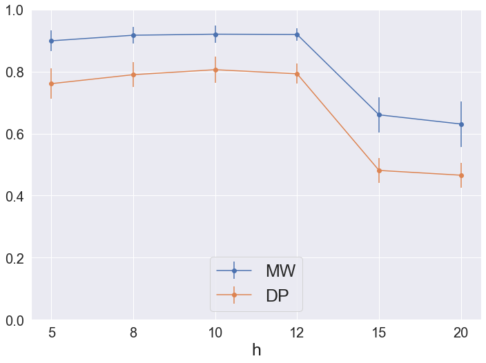
(a) Sensitivity of VaDE to the hidden dimension $h$ while we fix $k=10$

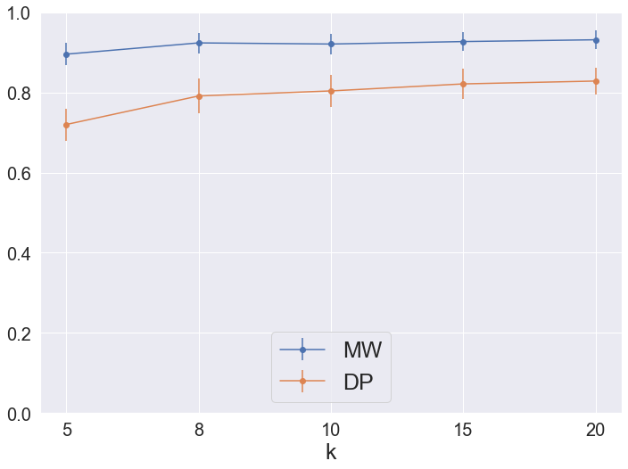
(b) Sensitivity of VaDE to the number of latent clusters $k$ while we fix $h=10$

Figure 4: Evaluating the sensitivity of VaDE on MNIST to its hyper-parameters $h$, which denotes the dimensionality of the latent space embedding, and $k$, which denotes the number of GMM components used for the latent space. We plot the Moseley-Wang objective (MW) and dendrogram purity (DP) as we vary either $h$ or $k$. Overall, we see that as long as $h$ is between 5 and 12, then the results are stable. Similarly, $k$ just needs to be at least 8. Therefore, while these parameters are important, the VaDE model is not very sensitive. Note that in our experiments for real data we fixed $h=10$ and for synthetic data we set $h$ to be the dimensionality of the BTGM (either $3,4,$ or $5$). For real/synthetic data we set $k$ to be the number of ground truth clusters (i.e., $k=10$ for MNIST).

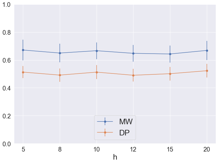
(a) Sensitivity of VAE to the hidden dimension $h$ with the same architecture as VaDE

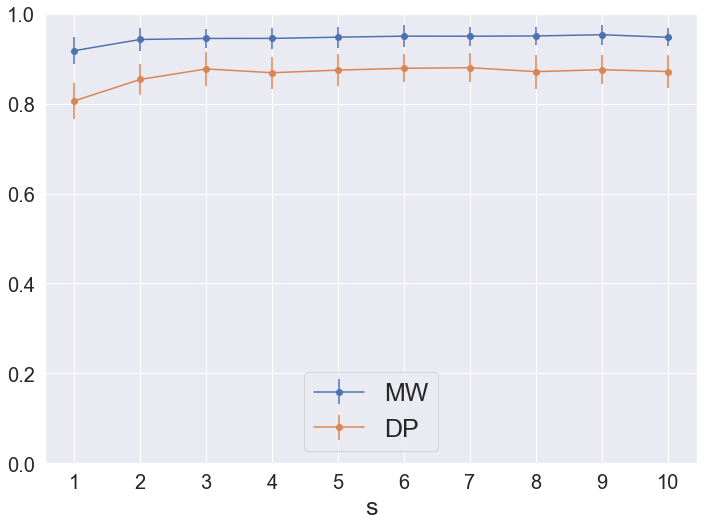
(b) Sensitivity of VaDE to the rescaling factor $s$ while we fix $h=10$ and $k=10$

Figure 5: On the left, we evaluate the sensitivity of VAE on MNIST to its hyper-parameters $h$, which denotes the dimensionality of the latent space embedding. On the right, we evaluate the sensitivity of VaDE + Trans to its hyper-parametere $s$. We plot the Moseley-Wang objective (MW) and dendrogram purity (DP) as we vary either $h$ or $s$. We see that the performance of VAE is not sensitive to its hidden dimension size $h$. But overall, the VAE does not perform well with respect to DP and MW. As for the rescaling experiment, we see that the effect of $s$ becomes stable when $s\geq 3$. Note that in the real dataset experiments we set $s=3$.

Comparing Linkage-Based Methods.   Table 4 shows the DP and MW results for several linkage-based variations, depending on the function used to determine cluster similarity. Overall, we see that Ward’s method performs the best on average. However, in some cases, the other methods do comparably.

Table 4: Dendrogram Purity and Moseley-Wang’s objective using different HAC linkage methods on VaDE + Transformed latent space.

	Dendro. Purity	M-W objective	Dendro. Purity	M-W objective
Single	0.829 $\pm$ 0.038	0.932 $\pm$ 0.023	0.260 $\pm$ 0.005	0.419 $\pm$ 0.006
Complete	0.854 $\pm$ 0.040	0.937 $\pm$ 0.024	0.293 $\pm$ 0.008	0.451 $\pm$ 0.016
Centroid	0.859 $\pm$ 0.035	0.949 $\pm$ 0.019	0.284 $\pm$ 0.008	0.453 $\pm$ 0.009
Average	0.866 $\pm$ 0.035	0.948 $\pm$ 0.023	0.295 $\pm$ 0.005	0.462 $\pm$ 0.006
Ward	0.870 $\pm$ 0.031	0.948 $\pm$ 0.025	0.300 $\pm$ 0.008	0.465 $\pm$ 0.011

MNIST

CIFAR-25-s

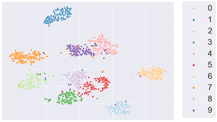
(a) $k=10$

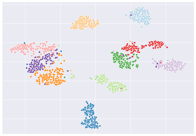
(b) $k=15$

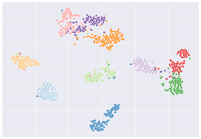
(c) $k=20$

Figure 6: tSNE visualization of the VaDE latent space with different numbers of latent clusters $k$. We can see that the latent space of VaDE becomes more separated as the number of clusters $k$ increases. When $k=20$, many of the original 10 clusters of digit further divide into 2 smaller clusters, which in total, form the 20 clusters learned by VaDE.

Dataset Details.   We conduct the experiments on our synthetic data from BTGM as well as real data benchmarks: Reuters [53], MNIST [48] and CIFAR-100 [45], 20 Newsgroup [47]. In the experiments, we only use 25 classes from CIFAR-100 that fall into one of the five superclasses "aquatic animals", "flowers", "fruits and vegetables", "large natural outdoor scenes" and "vehicle1" , we call it CIFAR-25. Below we also provide further details on the Digits dataset of handwritten digits . More details about the number of clusters and other statistics can be found in Table 5.

Rescaling explained.   The motivation of rescaling transformation can be explained using Figure 7. (a) shows the tSNE visualization of the VaDE embedding before and after the rescaling transformation. As we can see, each cluster becomes more separated. In (b), we visualize the inter-class distance matrices before and after the transformation. We use blue and black bounding boxes to highlight few superclusters revealed in the VaDE embedding. These high level structures remain unchanged after the rescaling, which is a consequence of property (ii) in Section 3.

Separability assumption.   It’s true that such a property does not hold for the real datasets before the embedding. But the assumptions of our theorems are not about the real data themselves, but about the transformed data after the VaDE embedding. We observe that VaDE increases the separation of data from different clusters. Indeed, we verify this for MNIST in Figure 8 below. We provide further justification for using VaDE via two new theorems that relate separability and Ward’s methods.

Table 5: Dataset Details.

	Digits	Reuters	MNIST	20newsgroup	CIFAR-25
# ground truth clusters	10	4	10	20	25
# data for training	6560	680K	60K	18K	15K
# data for evaluation	1000	10k	10k	18k	15k
Dimensionality	64	2000	768	2000	3072
Size of hidden dimension	5	10	10	20	20

C.1 Digits Dataset

There are few experimental results that evaluate dendrogram purity for the Digits dataset in previous papers. First we experiment using the same settings and same test set construction for Digits as in [58]. In this case, VaDE+Ward achieves a DP of 0.941, substantially improving the previous state-of-the-art results for dendrogram purity from existing methods: the DP of [58] is 0.675, the DP of PERCH [43] is 0.614, and the DP of BIRCH [88] is 0.544. In other words, our approach of VaDE+Ward leads to 26.5 point increase in DP for this simple dataset.

Surprisingly, we find that the test data they used is quite easy, as the DP and MW numbers are substantially better compared to using a random subset as the test set. Therefore, we follow the same evaluation settings as in Section 5 and randomly sampled 100 samples of 1000 data points for evaluation. The results are shown in Table 6. The contrast between the previous test data (easier) versus random sampling (harder) further supports our experimental set-up in the main paper.

Table 6: Dendrogram Purity and Moseley-Wang’s objective using different embedding methods in Digits dataset. Overall, VaDE + Trans. only provides a minor improvement in DP. Using Ward on the original space already achieves decent results.

	Dendro. Purity	M-W objective
Original	0.820 $\pm$ 0.031	0.846 $\pm$ 0.029
PCA	0.823 $\pm$ 0.028	0.844 $\pm$ 0.027
VaDE	0.824 $\pm$ 0.026	0.840 $\pm$ 0.024
VaDE + Trans.	0.832 $\pm$ 0.029	0.845 $\pm$ 0.024

(a)

(b)

Figure 7: (a) tSNE visualization of the embedded data for MNIST before and after the rescaling transformation, (b) shows the inter-class distance matrix before and after the rescaling transformation

Figure 8: Cluster separation is measured by $\displaystyle\sum_{x\in\mathcal{C}_{i}}\sum_{y\in\mathcal{C}_{j}}\left\lVert x-y\right\rVert\left(\sum_{x,y\in\mathcal{C}_{i}}\left\lVert x-y\right\rVert\right)^{-1/2}\left(\sum_{x,y\in\mathcal{C}_{j}}\left\lVert x-y\right\rVert\right)^{-1/2}$.

References

- [1] Amir Abboud, Vincent Cohen-Addad, and Hussein Houdrougé. Subquadratic high-dimensional hierarchical clustering. In Advances in Neural Information Processing Systems, pages 11576–11586, 2019.
- [2] Marcel R Ackermann, Johannes Blömer, Daniel Kuntze, and Christian Sohler. Analysis of agglomerative clustering. Algorithmica, 69(1):184–215, 2014.
- [3] Sameer Agarwal, Josh Wills, Lawrence Cayton, Gert Lanckriet, David Kriegman, and Serge Belongie. Generalized non-metric multidimensional scaling. In Artificial Intelligence and Statistics, pages 11–18, 2007.
- [4] Sara Ahmadian, Vaggos Chatziafratis, Alessandro Epasto, Euiwoong Lee, Mohammad Mahdian, Konstantin Makarychev, and Grigory Yaroslavtsev. Bisect and conquer: Hierarchical clustering via max-uncut bisection. arXiv preprint arXiv:1912.06983, 2019.
- [5] Elie Aljalbout, Vladimir Golkov, Yawar Siddiqui, Maximilian Strobel, and Daniel Cremers. Clustering with deep learning: Taxonomy and new methods. arXiv preprint arXiv:1801.07648, 2018.
- [6] Metin Balaban, Niema Moshiri, Uyen Mai, Xingfan Jia, and Siavash Mirarab. Treecluster: Clustering biological sequences using phylogenetic trees. PloS one, 14(8), 2019.
- [7] Sivaraman Balakrishnan, Min Xu, Akshay Krishnamurthy, and Aarti Singh. Noise thresholds for spectral clustering. In Advances in Neural Information Processing Systems, pages 954–962, 2011.
- [8] Maria-Florina Balcan, Travis Dick, and Manuel Lang. Learning to link. arXiv preprint arXiv:1907.00533, 2019.
- [9] Avrim Blum, John Hopcroft, and Ravindran Kannan. Foundations of data science. Cambridge University Press, 2020.
- [10] Ingwer Borg and Patrick JF Groenen. Modern multidimensional scaling: Theory and applications. Springer Science & Business Media, 2005.
- [11] Mathilde Caron, Piotr Bojanowski, Armand Joulin, and Matthijs Douze. Deep clustering for unsupervised learning of visual features. In Proceedings of the European Conference on Computer Vision (ECCV), pages 132–149, 2018.
- [12] Ines Chami, Albert Gu, Vaggos Chatziafratis, and Christopher Ré. From trees to continuous embeddings and back: Hyperbolic hierarchical clustering. arXiv preprint arXiv:2010.00402, 2020.
- [13] Moses Charikar and Vaggos Chatziafratis. Approximate hierarchical clustering via sparsest cut and spreading metrics. In Proceedings of the Twenty-Eighth Annual ACM-SIAM Symposium on Discrete Algorithms, pages 841–854. SIAM, 2017.
- [14] Moses Charikar, Vaggos Chatziafratis, Rad Niazadeh, and Grigory Yaroslavtsev. Hierarchical clustering for euclidean data. arXiv preprint arXiv:1812.10582, 2018.
- [15] Giovanni Chierchia and Benjamin Perret. Ultrametric fitting by gradient descent. In Advances in neural information processing systems, pages 3175–3186, 2019.
- [16] Fan Chung and Linyuan Lu. Complex graphs and networks, volume 107. American Mathematical Soc., 2006.
- [17] Vincent Cohen-Addad, Varun Kanade, and Frederik Mallmann-Trenn. Hierarchical clustering beyond the worst-case. In Advances in Neural Information Processing Systems, pages 6201–6209, 2017.
- [18] Sanjoy Dasgupta. Performance guarantees for hierarchical clustering. In International Conference on Computational Learning Theory, pages 351–363. Springer, 2002.
- [19] Sanjoy Dasgupta. A cost function for similarity-based hierarchical clustering. In Proceedings of the forty-eighth annual ACM symposium on Theory of Computing, pages 118–127, 2016.
- [20] Christopher De Sa, Albert Gu, Christopher Ré, and Frederic Sala. Representation tradeoffs for hyperbolic embeddings. Proceedings of machine learning research, 80:4460, 2018.
- [21] Nat Dilokthanakul, Pedro AM Mediano, Marta Garnelo, Matthew CH Lee, Hugh Salimbeni, Kai Arulkumaran, and Murray Shanahan. Deep unsupervised clustering with gaussian mixture variational autoencoders. arXiv preprint arXiv:1611.02648, 2016.
- [22] Ehsan Emamjomeh-Zadeh and David Kempe. Adaptive hierarchical clustering using ordinal queries. In Proceedings of the Twenty-Ninth Annual ACM-SIAM Symposium on Discrete Algorithms, pages 415–429. SIAM, 2018.
- [23] Maziar Moradi Fard, Thibaut Thonet, and Eric Gaussier. Deep -means: Jointly clustering with -means and learning representations. arXiv preprint arXiv:1806.10069, 2018.
- [24] William Feller. An introduction to probability theory and its applications. Vol. 1. John Wiley & Sons,, 1968.
- [25] Jhosimar Arias Figueroa and Adín Ramírez Rivera. Is simple better?: Revisiting simple generative models for unsupervised clustering. In Second workshop on Bayesian Deep Learning (NIPS), 2017.
- [26] Jerome Friedman, Trevor Hastie, and Robert Tibshirani. The elements of statistical learning, volume 1:10. Springer Series in Statistics, New York, 2001.
- [27] Octavian Ganea, Gary Becigneul, and Thomas Hofmann. Hyperbolic entailment cones for learning hierarchical embeddings. In International Conference on Machine Learning, pages 1646–1655, 2018.
- [28] Debarghya Ghoshdastidar, Michaël Perrot, and Ulrike von Luxburg. Foundations of comparison-based hierarchical clustering. In Advances in Neural Information Processing Systems, pages 7454–7464, 2019.
- [29] Jacob Goldberger and Sam T Roweis. Hierarchical clustering of a mixture model. In Advances in Neural Information Processing Systems, pages 505–512, 2005.
- [30] Prasoon Goyal, Zhiting Hu, Xiaodan Liang, Chenyu Wang, and Eric P Xing. Nonparametric variational auto-encoders for hierarchical representation learning. In Proceedings of the IEEE International Conference on Computer Vision, pages 5094–5102, 2017.
- [31] Anna Großwendt, Heiko Röglin, and Melanie Schmidt. Analysis of ward’s method. In Proceedings of the Thirtieth Annual ACM-SIAM Symposium on Discrete Algorithms, pages 2939–2957. SIAM, 2019.
- [32] Anna-Klara Großwendt. Theoretical Analysis of Hierarchical Clustering and the Shadow Vertex Algorithm. PhD thesis, Universität Bonn, 2020.
- [33] Albert Gu, Frederic Sala, Beliz Gunel, and Christopher Ré. Learning mixed-curvature representations in product spaces. In International Conference on Learning Representations, 2019.
- [34] Xifeng Guo, Xinwang Liu, En Zhu, and Jianping Yin. Deep clustering with convolutional autoencoders. In International conference on neural information processing, pages 373–382. Springer, 2017.
- [35] Katherine A Heller and Zoubin Ghahramani. Bayesian hierarchical clustering. In Proceedings of the 22nd international conference on Machine learning, pages 297–304, 2005.
- [36] Daniel Hsu. Columbia COMS 4772 Fall 2016, Lecture Notes: High-dimensional Gaussians, 2016. URL: https://www.cs.columbia.edu/~djhsu/coms4772-f16/lectures/gaussians.md.handout.pdf. Last visited on 2020/05/22.
- [37] Kevin G Jamieson and Robert D Nowak. Low-dimensional embedding using adaptively selected ordinal data. In 2011 49th Annual Allerton Conference on Communication, Control, and Computing (Allerton), pages 1077–1084. IEEE, 2011.
- [38] Zhuxi Jiang, Yin Zheng, Huachun Tan, Bangsheng Tang, and Hanning Zhou. Variational deep embedding: an unsupervised and generative approach to clustering. In Proceedings of the 26th International Joint Conference on Artificial Intelligence, pages 1965–1972, 2017.
- [39] Ehsan Kazemi, Lin Chen, Sanjoy Dasgupta, and Amin Karbasi. Comparison based learning from weak oracles. In International Conference on Artificial Intelligence and Statistics, pages 1849–1858, 2018.
- [40] Benjamin King. Step-wise clustering procedures. Journal of the American Statistical Association, 62(317):86–101, 1967.
- [41] Diederik P Kingma and Max Welling. Auto-encoding variational bayes. stat, 1050:1, 2014.
- [42] Alexej Klushyn, Nutan Chen, Richard Kurle, Botond Cseke, and Patrick van der Smagt. Learning hierarchical priors in vaes. In Advances in Neural Information Processing Systems, pages 2866–2875, 2019.
- [43] Ari Kobren, Nicholas Monath, Akshay Krishnamurthy, and Andrew McCallum. A hierarchical algorithm for extreme clustering. In Proceedings of the 23rd ACM SIGKDD International Conference on Knowledge Discovery and Data Mining, pages 255–264, 2017.
- [44] Samory Kpotufe and Ulrike von Luxburg. Pruning nearest neighbor cluster trees. In International Conference on Machine Learning (ICML), 2011.
- [45] Alex Krizhevsky. Learning multiple layers of features from tiny images. Technical report, University of Toronto, 2009.
- [46] Godfrey N Lance and William Thomas Williams. A general theory of classificatory sorting strategies: 1. hierarchical systems. The computer journal, 9(4):373–380, 1967.
- [47] Ken Lang. Newsweeder: Learning to filter netnews. In Proceedings of the Twelfth International Conference on Machine Learning, pages 331–339, 1995.
- [48] Y. Lecun, L. Bottou, Y. Bengio, and P. Haffner. Gradient-based learning applied to document recognition. Proceedings of the IEEE, 86(11):2278–2324, 1998.
- [49] Fengfu Li, Hong Qiao, and Bo Zhang. Discriminatively boosted image clustering with fully convolutional auto-encoders. Pattern Recognition, 83:161–173, 2018.
- [50] Xiaopeng Li, Zhourong Chen, Leonard KM Poon, and Nevin L Zhang. Learning latent superstructures in variational autoencoders for deep multidimensional clustering. In International Conference on Learning Representations, 2018.
- [51] Guolong Lin, Chandrashekhar Nagarajan, Rajmohan Rajaraman, and David P Williamson. A general approach for incremental approximation and hierarchical clustering. SIAM Journal on Computing, 39(8):3633–3669, 2010.
- [52] Nathan Linial, Eran London, and Yuri Rabinovich. The geometry of graphs and some of its algorithmic applications. Combinatorica, 15(2):215–245, 1995.
- [53] C. Goutte M.-R. Amini, N. Usunier. Learning from multiple partially observed views - an application to multilingual text categorization. In Advances in Neural Information Processing Systems, pages 28–36, 2009.
- [54] Christopher D Manning, Prabhakar Raghavan, and Hinrich Schütze. Introduction to information retrieval. Cambridge university press, 2008.
- [55] Emile Mathieu, Charline Le Lan, Chris J Maddison, Ryota Tomioka, and Yee Whye Teh. Continuous hierarchical representations with poincaré variational auto-encoders. In Advances in neural information processing systems, pages 12544–12555, 2019.
- [56] Erxue Min, Xifeng Guo, Qiang Liu, Gen Zhang, Jianjing Cui, and Jun Long. A survey of clustering with deep learning: From the perspective of network architecture. IEEE Access, 6:39501–39514, 2018.
- [57] Gal Mishne, Uri Shaham, Alexander Cloninger, and Israel Cohen. Diffusion nets. Applied and Computational Harmonic Analysis, 47(2):259–285, 2019.
- [58] Nicholas Monath, Manzil Zaheer, Daniel Silva, Andrew McCallum, and Amr Ahmed. Gradient-based hierarchical clustering using continuous representations of trees in hyperbolic space. In 25th ACM SIGKDD International Conference on Knowledge Discovery & Data Mining, pages 714–722, 2019.
- [59] Benjamin Moseley and Joshua Wang. Approximation bounds for hierarchical clustering: Average linkage, bisecting k-means, and local search. In Advances in Neural Information Processing Systems, pages 3094–3103, 2017.
- [60] Eric Nalisnick, Lars Hertel, and Padhraic Smyth. Approximate Inference for Deep Latent Gaussian Mixtures. In NIPS Workshop on Bayesian Deep Learning, 2016.
- [61] Eric Nalisnick and Padhraic Smyth. Stick-breaking variational autoencoders. In International Conference on Learning Representations (ICLR), 2017.
- [62] Maximillian Nickel and Douwe Kiela. Poincaré embeddings for learning hierarchical representations. In Advances in neural information processing systems (NIPS), pages 6338–6347, 2017.
- [63] Oliver Nina, Jamison Moody, and Clarissa Milligan. A decoder-free approach for unsupervised clustering and manifold learning with random triplet mining. In Proceedings of the IEEE International Conference on Computer Vision Workshops, pages 0–0, 2019.
- [64] Alan P Reynolds, Graeme Richards, Beatriz de la Iglesia, and Victor J Rayward-Smith. Clustering rules: a comparison of partitioning and hierarchical clustering algorithms. Journal of Mathematical Modelling and Algorithms, 5(4):475–504, 2006.
- [65] Danilo Jimenez Rezende, Shakir Mohamed, and Daan Wierstra. Stochastic backpropagation and approximate inference in deep generative models. In International Conference on Machine Learning (ICML), pages 1278–1286, 2014.
- [66] Maurice Roux. A comparative study of divisive and agglomerative hierarchical clustering algorithms. Journal of Classification, 35(2):345–366, 2018.
- [67] Ruslan Salakhutdinov, Joshua Tenenbaum, and Antonio Torralba. One-shot learning with a hierarchical nonparametric bayesian model. In Proceedings of ICML Workshop on Unsupervised and Transfer Learning, pages 195–206, 2012.
- [68] Rik Sarkar. Low distortion delaunay embedding of trees in hyperbolic plane. In International Symposium on Graph Drawing, pages 355–366. Springer, 2011.
- [69] Jingbo Shang, Xinyang Zhang, Liyuan Liu, Sha Li, and Jiawei Han. Nettaxo: Automated topic taxonomy construction from text-rich network. In Proceedings of The Web Conference 2020, pages 1908–1919, 2020.
- [70] Shweta Sharma, Neha Batra, et al. Comparative study of single linkage, complete linkage, and ward method of agglomerative clustering. In 2019 International Conference on Machine Learning, Big Data, Cloud and Parallel Computing (COMITCon), pages 568–573. IEEE, 2019.
- [71] Su-Jin Shin, Kyungwoo Song, and Il-Chul Moon. Hierarchically clustered representation learning. arXiv preprint arXiv:1901.09906, 2019.
- [72] Peter HA Sneath and Robert R Sokal. Numerical taxonomy. The principles and practice of numerical classification. W.H. Freeman, 1973.
- [73] Rishi Sonthalia and Anna C. Gilbert. Tree! i am no tree! i am a low dimensional hyperbolic embedding, 2020.
- [74] Gabor J Szekely and Maria L Rizzo. Hierarchical clustering via joint between-within distances: Extending ward’s minimum variance method. Journal of classification, 22(2), 2005.
- [75] Yee W Teh, Hal Daume III, and Daniel M Roy. Bayesian agglomerative clustering with coalescents. In Advances in Neural Information Processing Systems, pages 1473–1480, 2008.
- [76] Alexandru Tifrea, Gary Bécigneul, and Octavian-Eugen Ganea. Poincare GloVe: Hyperbolic Word Embeddings. arXiv preprint arXiv:1810.06546, 2018.
- [77] Eric K. Tokuda, Cesar H. Comin, and Luciano da F. Costa. Revisiting agglomerative clustering. arXiv preprint arXiv:2005.07995, 2020.
- [78] Jakub Tomczak and Max Welling. Vae with a vampprior. In International Conference on Artificial Intelligence and Statistics, pages 1214–1223, 2018.
- [79] Yao-Hung Hubert Tsai, Liang-Kang Huang, and Ruslan Salakhutdinov. Learning robust visual-semantic embeddings. In 2017 IEEE International Conference on Computer Vision (ICCV), pages 3591–3600. IEEE, 2017.
- [80] Elad Tzoreff, Olga Kogan, and Yoni Choukroun. Deep discriminative latent space for clustering. arXiv preprint arXiv:1805.10795, 2018.
- [81] Yiğit Uğur and Abdellatif Zaidi. Variational information bottleneck for unsupervised clustering: Deep gaussian mixture embedding. Entropy, 22(2):213, 2020.
- [82] Nuno Vasconcelos and Andrew Lippman. Learning mixture hierarchies. In Advances in Neural Information Processing Systems, pages 606–612, 1999.
- [83] Joe H Ward Jr. Hierarchical grouping to optimize an objective function. Journal of the American statistical association, 58(301):236–244, 1963.
- [84] Junyuan Xie, Ross Girshick, and Ali Farhadi. Unsupervised deep embedding for clustering analysis. In International conference on machine learning, pages 478–487, 2016.
- [85] Nishant Yadav, Ari Kobren, Nicholas Monath, and Andrew McCallum. Supervised hierarchical clustering with exponential linkage. In International Conference on Machine Learning (ICML), 2019.
- [86] Bo Yang, Xiao Fu, Nicholas D Sidiropoulos, and Mingyi Hong. Towards k-means-friendly spaces: Simultaneous deep learning and clustering. In Proceedings of the 34th International Conference on Machine Learning-Volume 70, pages 3861–3870. JMLR. org, 2017.
- [87] Chao Zhang, Fangbo Tao, Xiusi Chen, Jiaming Shen, Meng Jiang, Brian Sadler, Michelle Vanni, and Jiawei Han. Taxogen: Unsupervised topic taxonomy construction by adaptive term embedding and clustering. In Proceedings of the 24th ACM SIGKDD International Conference on Knowledge Discovery & Data Mining, pages 2701–2709, 2018.
- [88] Tian Zhang, Raghu Ramakrishnan, and Miron Livny. Birch: An efficient data clustering method for very large databases. In Proceedings of the 1996 ACM SIGMOD International Conference on Management of Data, SIGMOD ’96, page 103–114, New York, NY, USA, 1996. Association for Computing Machinery.