Constraining primordial black holes as dark matter at JUNO

Abstract

As an attractive candidate for dark matter, the PBH in the mass range ($8\times 10^{14}\sim 10^{16}$) $\mathrm{g}$ could be detected via their Hawking radiation, including neutrinos and antineutrinos of three flavors. In this paper, we investigate the possibility to constrain the PBH as dark matter by measuring (anti)neutrino signals at the large liquid-scintillator detector of Jiangmen Underground Neutrino Observatory (JUNO). Among six available detection channels, the inverse beta decay $\overline{\nu}_{e}+p\to e^{+}+n$ is shown to be most sensitive to the fraction $f_{\rm PBH}$ of PBH contributing to the dark matter abundance. Given the PBH mass $M_{\rm PBH}=10^{15}~{}{\rm g}$, we find that JUNO will be able to place an upper bound $f_{\rm PBH}\lesssim 3\times 10^{-5}$, which is 20 times better than the current best limit $f_{\rm PBH}\lesssim 6\times 10^{-4}$ from Super-Kamiokande. For heavier PBH with a lower Hawking temperature, the (anti)neutrinos become less energetic, leading to a relatively weaker bound.

I Introduction

The observations of gravitational waves by LIGO Abbott et al. (2016) have stimulated very active discussions on the origin of BBH. In particular, great interest in the primordial black holes (PBHs) as the seeds for the formation of BBH has been revived Bird et al. (2016); Wang et al. (2018); Mandic et al. (2016); Clesse and García-Bellido (2017a); Raidal et al. (2017); Cholis (2017); Clesse and García-Bellido (2017b); Cai et al. (2019); Sasaki et al. (2016). Recent studies Sasaki et al. (2016); Ali-Haïmoud et al. (2017); Chen and Huang (2018) have shown that the PBH scenario predicts a merger rate that is very consistent with the local observations. On the other hand, produced in the early Universe, PBH could be a viable candidate for cold dark matter Hawking (1971); Carr and Hawking (1974); Chapline (1975). The fraction of dark matter in the form of PBH is usually defined as $f_{\text{PBH}}=\Omega_{\text{PBH}}/\Omega_{\text{DM}}$, where $\Omega_{\text{PBH}}$ and $\Omega_{\text{DM}}$ denote the energy density fraction of PBH and that of dark matter in the present Universe, respectively. Various constraints on $f_{\text{PBH}}$ within a broad range of PBH masses have been derived in the literature. See recent reviews in Refs. Carr et al. (2020); Carr and Kuhnel (2020) and references therein.

The Hawking radiation Hawking (1975) of the PBH has been suggested for experimental observations and can be used to explore the intrinsic properties of PBH Boudaud and Cirelli (2019); Dasgupta et al. (2020); Arbey et al. (2019); Carr et al. (2009); Laha (2019); Laha et al. (2020); Ballesteros et al. (2020); Lunardini and Perez-Gonzalez (2020). As is well known, the black holes could emit particles near their event horizons, and the black hole evaporates faster as its mass decreases Page (1976); Macgibbon and Webber (1990); Macgibbon (1991). For a PBH, depending on its formation time, it could have a much smaller mass than ordinary stars Hawking (1971); Carr and Hawking (1974). The PBH with masses $M_{\mathrm{PBH}}\lesssim\mathcal{O}(10^{15})~{}\mathrm{g}$ would have evaporated over at the present age of the Universe Hawking (1975). Based on the experimental searches for the Hawking radiation, stringent constraints on $f_{\text{PBH}}$ within a mass range $(10^{14}\sim 10^{17})~{}\mathrm{g}$ have been obtained (see, e.g., Refs. Carr et al. (2020); Carr and Kuhnel (2020), for recent reviews). For example, there exists an upper limit $f_{\text{PBH}}\lesssim 10^{-7}$ for $M_{\mathrm{PBH}}\simeq 10^{15}\text{g}$ through an observation of the $e^{\pm}$ flux from Voyager 1 Boudaud and Cirelli (2019). By observing the $\gamma$-ray lines from the $e^{-}$-$e^{+}$ annihilation and the isotropic diffuse $\gamma$-ray background, respectively, INTEGRAL Siegert et al. (2016) and FERMI-LAT Ackermann et al. (2015) have restricted $f_{\text{PBH}}$ to be less than $10^{-3}$ for $M_{\mathrm{PBH}}=10^{16}\text{g}$ Dasgupta et al. (2020); Arbey et al. (2019). Reference Dasgupta et al. (2020), also shows that an upper limit $f_{\text{PBH}}\lesssim 6\times 10^{-4}$ for $M_{\mathrm{PBH}}\simeq 10^{15}~{}\text{g}$ can be derived via the neutrino observation from Super-K Bays (2012).

As a multipurpose neutrino experiment with a 20 kton liquid-scintillator (LS) detector, JUNO An et al. (2015) will be able to detect low-energy astrophysical neutrinos in addition to reactor electron-antineutrinos. The primary reaction channels for astrophysical neutrinos at JUNO include the inverse beta decay $\overline{\nu}_{e}+p\to e^{+}+n$ (IBD), the elastic neutrino-proton scattering $\nu+p\to\nu+p$ ($p$ES), the elastic neutrino-electron scattering $\nu_{e}+e^{-}\to\nu_{e}+e^{-}$ ($e$ES), and the neutrino-nucleus (i.e., ${{}^{12}}{\rm C}$) reactions $\nu+{{}^{12}}{\rm C}\to\nu+{{}^{12}}{\rm C}^{*}$, $\nu_{e}+{{}^{12}}{\rm C}\to e^{-}+{{}^{12}}{\rm N}$, and $\overline{\nu}_{e}+{{}^{12}}{\rm C}\to e^{+}+{{}^{12}}{\rm B}$. With a perfect neutron-tagging efficiency of the LS detector, JUNO is expected to have a great potential to discover the DSNB An et al. (2015). As mentioned above, the upper limit on the DSNB flux from Super-K has been used to constrain $f_{\text{PBH}}$ for small-mass PBH Dasgupta et al. (2020). Therefore, we are very motivated to investigate how restrictive the bound on $f_{\rm PBH}$ from JUNO will be. Compared to Super-K, we expect that JUNO could improve the constraint on $f_{\mathrm{PBH}}$ due to its more powerful neutron tagging, lower energy threshold, and better energy resolution. A similar analysis can be performed for the future Gadolinium-doping upgrade of Super-K.

The remaining part of this paper is organized as follows. In Sec. II, we calculate the neutrino fluxes from PBH in the Galactic and extragalactic dark matter halos. Then, Sec. III is devoted to the event spectra for all six neutrino detection channels at JUNO and the estimation of the relevant backgrounds. In Sec. IV, by comparing between the signals and backgrounds, we draw the upper limit on $f_{\rm PBH}$ from JUNO. Our main conclusions are finally summarized in Sec. V.

II Neutrino fluxes from PBH

Generally speaking, there are two different contributions, i.e., the primary and secondary components, to the neutrino fluxes from the evaporating PBH. The former arises directly from the Hawking radiation, while the latter stems from the decays of the secondary particles produced in the Hawking radiation Carr et al. (2009); Arbey and Auffinger (2019). For an evaporating PBH, the number of (anti)neutrinos ($N$) in unit energy ($E$) and time ($t$) is given by

$$\frac{{\rm d}^{2}N}{{\rm d}E{\rm d}t}=\frac{{\rm d}^{2}N}{{\rm d}E{\rm d}t}\Bigg{|}_{\text{pri}}+\frac{{\rm d}^{2}N}{{\rm d}E{\rm d}t}\Bigg{|}_{\text{sec}}\;,$$ (1)

where the first and second terms on the right-hand side denote the primary and secondary components, respectively. In our calculations, both components are evaluated by using BLACKHAWK Arbey and Auffinger (2019). It is worthwhile to notice that the spins of PBH in the present work are assumed to be negligible, as predicted by a class of theories for the PBH production Chiba and Yokoyama (2017); Mirbabayi et al. (2020).

Then the differential fluxes of (anti)neutrinos radiated from PBH can be calculated by taking into account the distribution and cosmological evolution. In units of $\text{cm}^{-2}~{}\text{s}^{-1}~{}\text{MeV}^{-1}$, they can be decomposed as follows

$$\frac{{\rm d}F}{{\rm d}E}=\frac{{\rm d}F_{\text{Gal}}}{{\rm d}E}+\frac{{\rm d}F_{\text{EG}}}{{\rm d}E}\;,$$ (2)

where the first and second terms at the right-hand side are contributed by PBH located in the Galactic and extragalactic dark halos, respectively.

For the extragalactic PBH, the differential (anti)neutrino flux can be written as Dasgupta et al. (2020); Carr et al. (2009)

$$\begin{split}\frac{{\rm d}F_{\text{EG}}}{{\rm d}E}=\int_{t_{\text{min}}}^{t_{\text{max}}}&{\rm d}t\ [1+z(t)]\frac{f_{\text{PBH}}\rho_{\text{DM}}}{M_{\text{PBH}}}\\ &\times\frac{{\rm d}^{2}N}{{\rm d}E_{\rm s}{\rm d}t}\bigg{|}_{E_{\rm s}=[1+z(t)]E}\;.\end{split}$$ (3)

According to the Planck 2018 results Aghanim et al. (2018), we set the average energy density of dark matter in the present Universe to be $\rho_{\text{DM}}=2.35\times 10^{-30}~{}\text{g}~{}\text{cm}^{-3}$. The (anti)neutrino energy at the source has been denoted as $E_{\rm s}$, while that in the observer’s frame has been denoted as $E$. The connection between them is given by $E_{\rm s}=[1+z(t)]E$, where the redshift $z(t)$ is a function of the cosmic time $t$ and encodes the cosmological evolution. For the lower and upper limits of the integration over the cosmic time in Eq. (3), we take the following values. First, the (anti)neutrinos emitted from the PBH in the very early time will be significantly redshifted. This causes that these (anti)neutrinos have extremely low energies today and cannot be detected. There is an exception for high-energy (anti)neutrinos, whose fluxes, however, are highly suppressed for the PBH masses of our interest. Therefore, we fix $t_{\text{min}}=10^{11}~{}\text{s}$ close to the epoch of radiation-matter equality and numerically confirm that changing $t_{\rm min}$ to be smaller has essentially no impact on the final results. Second, we choose $t_{\text{max}}=\text{min}\{\tau_{0},\tau_{\text{PBH}}\}$, where $\tau_{0}$ is the age of the Universe, $\tau_{\text{PBH}}$ is the lifetime of PBH, and the function $\text{min}\{x_{1},x_{2}\}$ singles out the smaller one from $x_{1}$ and $x_{2}$.

For the PBH in the Galactic dark halo, the differential (anti)neutrino flux can be calculated as Dasgupta et al. (2020)

$$\frac{{\rm d}F_{\mathrm{Gal}}}{{\rm d}E}=\int\frac{{\rm d}\Omega}{4\pi}\int_{0}^{l_{\text{max}}}{\rm d}l~{}\frac{{\rm d}^{2}N}{{\rm d}E{\rm d}t}\frac{f_{\text{PBH}}~{}\rho_{\text{Gal}}[r(l,\psi)]}{M_{\text{PBH}}}\;,$$ (4)

where $r(l,\psi)\equiv\sqrt{r^{2}_{\odot}-2lr_{\odot}\cos\psi+l^{2}}$ is the galactocentric distance calculated from the distance of the Earth to the Galactic center $r_{\odot}=8.5~{}{\rm kpc}$ and the line-of-sight distance $l$ to the PBH, with $\psi$ being the angle between these two directions. In addition, the angular integration is defined as $\int{\rm d}\Omega=\int_{0}^{2\pi}{\rm d}\phi\int_{0}^{\pi}{\rm d}\psi\sin\psi$ with $\phi$ being the azimuthal angle, and $\rho_{\text{MW}}(r)$ is the local energy density of dark matter. The maximal value of $l$ is determined by $l_{\text{max}}=({r^{2}_{\rm h}-r^{2}_{\odot}\sin^{2}\psi})^{1/2}+r_{\odot}\cos\psi$ with the halo radius $r_{\rm h}=200~{}{\rm kpc}$. For illustration, we implement the NFW profile Ng et al. (2014)

$$\rho_{\text{NFW}}(r)=0.4\times\left(\frac{8.5}{r}\right)\left(\frac{1+{8.5}/{20}}{1+{r}/{20}}\right)^{2}\ ,$$ (5)

which is in units of $\text{GeV}\cdot\text{cm}^{-3}$, and the distance $r$ is in units of kpc.

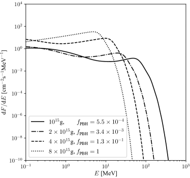
Figure 1: The differential (anti)neutrino flux from PBH for $M_{\rm PBH}=10^{15}~{}{\rm g}$ (solid curve), $2\times 10^{15}~{}{\rm g}$ (dot-dashed curve), $4\times 10^{15}~{}{\rm g}$ (dashed curve) and $8\times 10^{15}~{}{\rm g}$ (dotted curve), where the monochromatic mass function of PBH is assumed and the upper limit on $f_{\rm PBH}$ from Super-K Dasgupta et al. (2020) is input. The horizontal axis represents the (anti)neutrino energy in units of $\mathrm{MeV}$ at the detector, while the vertical one denotes the differential (anti)neutrino flux in units of $\text{cm}^{-2}~{}\text{s}^{-1}~{}\text{MeV}^{-1}$.

In Fig. 1, we show the differential fluxes of $\nu_{e}$ emitted from PBH for four benchmark masses within the range $(10^{15}\sim 10^{16})~{}\mathrm{g}$. The results for neutrinos and antineutrinos of other flavors are quite similar, as a consequence of the thermal Hawking radiation. In the numerical calculations, we have assumed a monochromatic mass function of PBH and taken the existing upper limit of $f_{\rm PBH}$ from Super-K Dasgupta et al. (2020). As one can observe from Fig. 1, neutrinos and antineutrinos from smaller-mass PBH have higher energies, mainly due to the higher Hawking temperature, while the magnitude of the fluxes is limited by the existing bound on $f_{\rm PBH}$.

Note that we have assumed neutrinos to be Majorana particles, and will calculate the event spectra in the next section in this case as well. The difference between the cases of Majorana and Dirac neutrinos will be clarified in Sec. IV.

III Event Spectra and Backgrounds

Given the (anti)neutrino fluxes radiated by PBH, we can figure out the event spectra for six available detection channels in the LS detector of JUNO. In this section, we present the results of the event spectra and estimate the relevant backgrounds at JUNO.

III.1 IBD channel

For the IBD channel $\overline{\nu}_{e}+p\to e^{+}+n$, both the final-state $e^{+}$ and $n$ can be perfectly observed in the LS detector. At JUNO, the event spectrum of IBD is given by Li et al. (2017)

$$\frac{{\rm d}N}{{\rm d}E_{0}}=N_{p}T\int_{E^{\rm thr}_{\rm IBD}}^{\infty}\sigma^{\text{IBD}}_{{\bar{\nu}_{e}}}(E)\frac{\rm dF}{\rm dE}\Big{|}_{\bar{\nu}_{e}}\mathcal{G}(E_{0};E_{\rm v},\delta_{E}){\rm d}E\;,$$ (6)

where the energy threshold for the IBD reaction is $E^{\rm thr}_{\rm IBD}=1.8~{}{\rm MeV}$, $E_{0}$ is the observed energy, $\mathcal{G}(E_{0};E_{\rm v},\delta_{E})$ is a Gaussian function of $E_{0}$ with an expectation value $E_{\rm v}$ and the standard deviation $\delta_{E}=3\%/\sqrt{E_{0}/\text{MeV}}$, i.e., the energy resolution of JUNO An et al. (2015); Li et al. (2017). The visible energy in the detector $E_{\rm v}=m_{e}+E_{e^{+}}$ arises from the annihilation of the final-state positrons with ambient electrons, where $m_{e}=0.511~{}{\rm MeV}$ is the electron mass. The IBD cross section $\sigma^{\text{IBD}}_{{\bar{\nu}_{e}}}$ and the positron energy $E_{e^{+}}$ depend on the antineutrino energy $E$ in the differential flux ${\rm d}F/{\rm d}E$ defined in Eq. (2). We obtain the dependency relation in Table 1 of Ref. Strumia and Vissani (2003). The total number $N_{p}$ of target protons in the LS and the effective running time $T$ in Eq. (6) can be found in Ref. Li et al. (2017).

With the differential fluxes of $\overline{\nu}_{e}$ in Fig. 1, we compute the IBD event spectra by using Eq. (6) and present the final results in Fig. 2, where different curves correspond to four benchmark PBH masses in Fig. 1. In our calculations, the fiducial mass of the JUNO detector is taken to be $20$ kton and the operation time is set to $T=10~{}{\rm yr}$. In Fig. 2, we can observe that the peak of the event spectrum moves toward lower energies as the PBH mass increases. It should be noticed that the peak rate is limited by the existing upper bound on $f_{\text{PBH}}$.

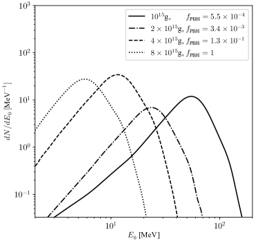
Figure 2: The IBD event spectra for PBH of four benchmark masses as in Fig. 1. For the LS detector, we have assumed the fiducial mass of $20$ kton and the effective running time of $10$ years. The horizontal axis refers to the observed energy in units of MeV, while the vertical one to the event spectrum in units of $\text{MeV}^{-1}$.

The main backgrounds for the IBD channel can be divided into four categories. The first one is the irreducible background from reactor antineutrinos, which dominate over others in the energy range below $12~{}\text{MeV}$ An et al. (2015); Li et al. (2020). From Fig. 2, we notice that when the PBH mass is $8\times 10^{15}~{}\text{g}$ or larger, the peaks of the event spectra shift to the region $E_{0}\lesssim 10~{}\text{MeV}$. Consequently, for $M_{\rm PBH}\gtrsim 8\times 10^{15}\text{g}$, the IBD signal will be severely contaminated by the reactor antineutrino background. For this reason, we mainly focus on the PBH with smaller masses or set an energy cut $E_{0}\gtrsim 12~{}{\rm MeV}$ to get rid of this background. The second one is DSNB, which is one the primary goals of Super-K and JUNO An et al. (2015). For illustration, we take into account the DSNB $\overline{\nu}_{e}$ flux with an average energy $\langle E_{\bar{\nu}_{e}}\rangle=15~{}\text{MeV}$. The third type of background is composed of the atmospheric neutrino charged-current (atm.CC) background and neutral-current (atm.NC) background. The former is caused by the IBDs of atmospheric neutrino $\bar{\nu}_{e}$, while the latter by the NC reactions of high-energy atmospheric (anti)neutrinos in the LS An et al. (2015); Gando et al. (2012). Both kinds of event spectra have been studied in Ref. An et al. (2015). The fourth background is the fast neutrons (FNs), which are produced by the cosmic high-energy muons arriving at the detector and induce the IBD-like events An et al. (2015). For the last two categories of backgrounds, the dedicated method of PSD has to be utilized, as we shall explain below.

$M_{\rm PBH}$[g]	$10^{15}$		$2\times 10^{15}$		$4\times 10^{15}$		$8\times 10^{15}$
$f_{\text{PBH}}$ (Super-K constraints)	$5.5\times 10^{-4}$		$3.4\times 10^{-3}$		$1.3\times 10^{-1}$		$1$
Energy window [MeV]	$[12,130]$		$[12,80]$		$[12,40]$		$[12,20]$
PSD procedure	Before	After	Before	After	Before	After	Before	After
PBH signal	$541.88$	$270.94$	$137.59$	$68.80$	$203.07$	$101.54$	$7.79$	$3.90$
Atm.NC	$1333.34$	$14.67$	$1105.10$	$12.16$	$746.71$	$8.21$	$348.24$	$3.83$
Atm.CC	$33.31$	$16.66$	$17.36$	$8.68$	$3.79$	$1.90$	$0.46$	$0.23$
DSNB	$17.72$	$8.86$	$17.72$	$8.86$	$17.72$	$8.86$	$12.20$	$6.10$
FN	$83.78$	$1.42$	$48.28$	$0.82$	$19.88$	$0.34$	$5.68$	$0.10$
Total backgrounds	$1468.15$	$41.61$	$1188.46$	$30.52$	$788.10$	$19.31$	$366.58$	$10.26$
$f_{\text{PBH}}$ (JUNO constraints)	$2.1\times 10^{-5}$		$4.4\times 10^{-4}$		$9.0\times 10^{-3}$		$1$

Table 1: Summary of the upper limits of the IBD event rates according to the Super-K constrain, the background rates estimation according to the corresponding mass of PBH energy windows from JUNO detector, the comparison of before and after PSD cut application, and the $f_{\text{PBH}}$ constrain estimation from JUNO backgrounds. The event rates are given in units of counts per $10$ year per $20$ kton.

Similar to the DSNB searches in the LS detectors, the PSD approach is critically important to enhance the SNR. Both signals and backgrounds in the LS will be finally converted into light, which can be observed by the photomultiplier tubes. For the light signals generated in different processes, the probability density functions of the photon emission time can be described as Möllenberg et al. (2015)

$$F(t)=\sum_{i}\frac{N_{i}}{\tau_{i}}e^{-t/\tau_{i}}\;,$$ (7)

where $i$ refers to the fast, slow and slower components, and $N_{i}$ and $\tau_{i}$ denote the fraction and time constant of $i$-th component, respectively. Then one can in principle identify different particles by the corresponding distribution functions $F(t)$. To make use of the tail-to-total ratio Möllenberg et al. (2015), we define the working parameter PSD as

$$\text{PSD}=\frac{\displaystyle\int_{t_{\text{cut}}}^{\infty}F(t){\rm d}t}{\displaystyle\int_{0}^{\infty}F(t){\rm d}t}\;,$$ (8)

where $t_{\text{cut}}$ denotes a cutoff time. For the signal and one kind of the relevant backgrounds, one can properly choose the cutoff time in order to reduce the number of background events more than that of the signal events.

For JUNO, Ref. An et al. (2015) has estimated the PSD efficiency, which is the fraction of events surviving the PSD procedure, $\epsilon_{\nu}=0.5$, $\epsilon_{\text{NC}}=0.011$, and $\epsilon_{\text{FN}}=0.017$.

In Table 1, we summarize the total number of IBD events from PBH and that of relevant backgrounds, where both the results before and after applying the PSD approach have been shown for comparison. The IBD events from PBH are calculated as in Fig. 2, and the backgrounds are categorized as in previous discussions. Comparing the total backgrounds before and after applying the PSD approach, we find a significant reduction of the backgrounds. One can notice that the dominant background is due to atm.NC, and for $M_{\rm PBH}>10^{15}~{}\text{g}$, the SNR without the PSD procedure are too small for any realistic observations.

III.2 $e$ES channel

For the $e$ES channel $\nu+e^{-}\to\nu+e^{-}$, all species of neutrinos and antineutrinos could contribute and the event spectrum can be calculated as Li et al. (2017)

$$\begin{split}\frac{{\rm d}N}{{\rm d}E_{0}}=&N_{e}T\sum_{\alpha}\int_{0}^{\infty}{\rm d}T_{e}\mathcal{G}(E_{0};T_{e},\delta_{E})\\ &\times\int_{E_{e}^{\text{min}}}^{\infty}\frac{{\rm d}F}{{\rm d}E}\bigg{|}_{\alpha}\frac{{\rm d}\sigma^{e\text{ES}}_{\nu_{\alpha}}(E)}{{\rm d}T_{e}}{\rm d}E\;,\end{split}$$ (9)

where the $e$ES cross section is $\sigma^{e\text{ES}}_{\nu_{\alpha}}$ with $\alpha$ standing for neutrinos and antineutrinos of three flavors, and $T_{e}$ is the electron kinetic energy. The minimal neutrino energy to produce a recoil electron energy $T_{e}$ is determined by $E_{e}^{\text{min}}\simeq T_{e}/2+\sqrt{T_{e}(T_{e}+2m_{e})}/2$. In addition, we should set $N_{e}=N_{p}$ due to the electric neutrality of the LS materials.

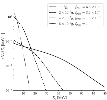
Figure 3: The $e$ES event spectra induced by PBH for four benchmark masses corresponding to those in Fig. 2, where the effective running time of $10$ years and the fiducial LS mass of $20$ kton have been assumed.

The $e$ES event spectra from PBH are shown in Fig. 3, where four benchmark masses for the PBH corresponding to those in Fig. 2 have been taken and the effective running time of 10 years and the fiducial LS mass of 20 kton have been assumed. As one can observe from Fig. 3, the maximal rate reaches $1.5~{}{\rm MeV}^{-1}$ for $M_{\rm PBH}=8\times 10^{15}~{}{\rm g}$ at the low-energy end. However, for the electron recoil events, there are numerous backgrounds from the ⁸B solar neutrino and other three types of cosmogenic isotopes (i.e., ¹¹C, ¹⁰C, and ¹¹Be). According to Ref. An et al. (2015), the total background events are estimated to $10^{4}\ \text{MeV}^{-1}$ per $10$ years per $20$ kton at JUNO. Compared with this background rate, the $e$ES event rates shown in Fig. 3 are much smaller. Therefore, it seems impossible to observe the $e$ES signals from PBH at the LS detectors.

III.3 $p$ES channel

As the advantages of the low energy threshold of the LS detectors, the $p$ES channel $\nu+p\to\nu+p$ can also be used to observe astrophysical neutrinos. The $p$ES event spectrum is computed as follows Li et al. (2017)

$$\begin{split}\frac{{\rm d}N}{{\rm d}E_{0}}=&N_{p}T\int{\rm d}T_{p}^{\prime}\mathcal{G}(E_{0};T_{p}^{\prime},\delta_{E})\\ &\times\sum_{\alpha}\frac{{\rm d}T_{p}}{{\rm d}T_{p}^{\prime}}\int_{E_{p}^{\text{min}}}^{\infty}\frac{{\rm d}F}{{\rm d}E}\bigg{|}_{\alpha}\frac{{\rm d}\sigma^{p\text{ES}}_{\nu_{\alpha}}(E)}{{\rm d}T_{p}}{\rm d}E\;,\end{split}$$ (10)

where ${\rm d}\sigma^{p{\rm ES}}_{\nu_{\alpha}}/{\rm d}T_{p}$ denotes the differential cross section with $T_{p}$ being the proton recoil energy. The minimal neutrino energy required to produce the final-state proton with a recoil energy of $T_{p}$ is approximately determined by $E_{p}^{\text{min}}=(T_{p}m_{p}/2)^{1/2}$ with $m_{p}=938.27~{}{\rm MeV}$ being the proton mass. However, the proton recoil energy will be quenched in the LS and observed as $T_{p}^{\prime}$, which is related to $T_{p}$ by the Birks law Li et al. (2017); Beacom et al. (2002). The quenching effects on recoiled protons in the LS have been shown numerically in Fig. 30 of Ref. An et al. (2015) and will be taken into account in our calculations.

Since the recoil energies of protons are small and the observed energies after quenching effects become even smaller, we consider only the (anti)neutrinos from the PBH with a mass of $M_{\rm PBH}=10^{15}~{}{\rm g}$, for which the (anti)neutrino energies are much higher than those for larger PBH masses. The final result has been presented in Fig. 4, from which one can see that the observed energy turns out to be located in the range of $(0.2\sim 1.8)~{}\text{MeV}$. Below $1~{}\text{MeV}$, the background is mainly caused by the radioactive decays of the LS materials and surroundings, whose rate has been estimated to be about $80$ events per $10$ sec An et al. (2015). In contrast, the $p$ES event rate produced by PBH is small, as one can observe from Fig. 4. It should be noticed that the operation time for the LS in Fig. 4 has been taken to be 10 years, together with the fiducial LS mass of $20$ kton. For the observed energy higher than $1\text{MeV}$, the rate for possible backgrounds has not been given in Ref. An et al. (2015), but the signal rate is highly suppressed, rendering the realistic observation to be difficult.

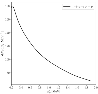
Figure 4: The $p$ES event spectrum induced by the (anti)neutrinos from the PBH of $M_{\rm PBH}=10^{15}~{}\text{g}$, $f_{\rm PBH}=5.5\times 10^{-4}$, where the effective running time of $10$ years and the fiducial LS mass of $20$ kton have been assumed.

III.4 ¹²C channel

There are three different reaction channels for the interaction between astrophysical neutrinos with the ¹²C nuclei in the LS detectors. The first one is the NC reaction $\nu+{{}^{12}}{\rm C}\to\nu+{{}^{12}}{\rm C}^{*}$, where the final-state nucleus resides in the excited state $(15.1~{}\text{MeV},1^{+})$ and its deexcitation leads to a gamma ray of $15.1~{}{\rm MeV}$ that can be registered in the detector. The NC event spectrum is given by

$$\begin{split}\frac{{\rm d}N}{{\rm d}E_{0}}=&N_{\text{C}}T\sum_{\alpha}\int{\rm d}E\sigma^{\text{NC}}_{\nu_{\alpha}}(E)\frac{{\rm d}F}{{\rm d}E}\bigg{|}_{\alpha}\\ &\times\mathcal{G}(E_{0};15.1~{}\text{MeV},\delta_{E})\;,\end{split}$$ (11)

where $N_{\rm C}=3N_{e}/23$ is the total number of ¹²C nuclei in the LS target Jia et al. (2019) and $\sigma^{\text{NC}}_{\nu_{\alpha}}$ denotes the total cross section. The other two are CC reactions, namely, $\nu_{e}+{{}^{12}}\text{C}\to e^{-}+{{}^{12}}\text{N}$ and $\overline{\nu}_{e}+{{}^{12}}\text{C}\to e^{+}+{{}^{12}}\text{B}$. The CC event spectrum is found to be

$$\begin{split}\frac{{\rm d}N}{{\rm d}E_{0}}=N_{\text{C}}T\int{\rm d}E&\sigma^{\text{CC}}_{\nu_{e}(\overline{\nu}_{e})}(E)\frac{{\rm d}F}{{\rm d}E}\bigg{|}_{\nu_{e}(\overline{\nu}_{e})}\\ &\times\mathcal{G}(E_{0};T_{e},\delta_{E})\;,\end{split}$$ (12)

where $T_{e}$ is the recoil energy of the final-state electron (or positron) and $\sigma^{\text{CC}}_{\nu_{e}}$ and $\sigma^{\rm CC}_{\overline{\nu}_{e}}$ denotes respectively the cross section of $\nu_{e}$-${{}^{12}}{\rm C}$ and $\overline{\nu}_{e}$-${{}^{12}}{\rm C}$ reaction. Moreover, we have $T_{e}=E_{\nu_{e}}-16.827~{}\text{MeV}$ for the ${}^{12}\text{C}(\nu_{e},e^{-})^{12}\text{N}$ channel while $T_{e}=E_{\overline{\nu}_{e}}-13.880~{}\text{MeV}$ for the ${}^{12}\text{C}(\overline{\nu}_{e},e^{+})^{12}\text{B}$ channel Fukugita et al. (1988). The cross sections of all three neutrino-carbon reaction channels can be found in Table 1 of Ref. Fukugita et al. (1988).

Figure 5: The event spectrum of the NC neutrino-¹²C reaction for the PBH of $M_{\rm PBH}=10^{15}~{}\text{g}$, $f_{\rm PBH}=5.5\times 10^{-4}$, where the effective running time of $10$ years and the fiducial LS mass of $20$ kton are taken.

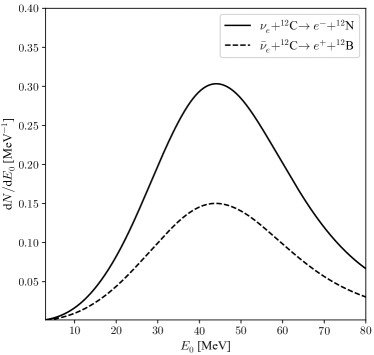
Figure 6: The event spectra of the CC reactions with ${{}^{12}}{\rm C}$ for the PBH of $M_{\rm PBH}=10^{15}~{}\text{g}$, $f_{\rm PBH}=5.5\times 10^{-4}$, where the effective running time of $10$ years and the fiducial LS mass of $20$ kton are taken.

Similar to the $p$ES channel, only high-energy neutrinos and antineutrinos can produce the signals with energies observable in the LS detectors. Therefore, we consider only the PBH with the lightest mass, i.e., $M_{\text{PBH}}=10^{15}~{}\text{g}$. The event spectra of NC and CC reactions are shown in Fig. 5 and Fig. 6, respectively, where the effective operation time of $10$ years and the fiducial LS mass of $20$ kton have been taken as before. In comparison with the IBD channel, the event rates in the ¹²C channel are much smaller and will not contribute much to the detection of PBH.

IV Constraints from JUNO

In the previous discussions, we have demonstrated that the IBD channel is most sensitive to the antineutrino signals from the PBH as dark matter. For this reason, only the IBD signal will be implemented to derive the constraints on the PBH at JUNO in this section. By requiring the signal-to-noise ratio $\text{\ac{SNR}}\geq 1.6/\sqrt{N}$ (i.e. 90% C.L.), where $N$ is the total event number of backgrounds for 10 years, we have shown the upper limit on $f_{\text{PBH}}$ for a given $M_{\text{PBH}}$ in Fig. 7. The solid curve stands for the constraint from JUNO in the case of Majorana neutrinos. For comparison, the currently best limit on $f_{\text{PBH}}$ from Super-K has been plotted the dot-dashed curve and the shaded area in light grey has been excluded Dasgupta et al. (2020). Two important observations can be made. First, after running for 10 years, JUNO will have the capability to explore the dark grey area in Fig. 7, which has not been constrained by current neutrino observatories. To be specific, given $M_{\rm PBH}=10^{15}~{}{\rm g}$, the upper limit $f_{\rm PBH}\lesssim 3\times 10^{-5}$ can be obtained from JUNO, which is about twenty times better than that $f_{\rm PBH}\lesssim 6\times 10^{-4}$ from Super-K. Second, JUNO will be able to constrain the PBH dark matter in the mass range $M_{\rm PBH}=(5\sim 8)\times 10^{15}~{}\text{g}$, for which $f_{\rm PBH}=1$ is still allowed by Super-K. As we have mentioned before, although there exist other observational limits on $f_{\rm PBH}$ from cosmic gamma rays, the neutrino observations will not only provide an independent limit on $f_{\rm PBH}$ but also a novel way to probe the mechanism of Hawking radiation of PBH.

Now we consider the difference between Majorana and Dirac neutrinos. The key point is that the evaporation rate of PBHs depends on the total number of degrees of freedom in the neutrino sector, which is $n^{\rm M}_{\rm dof}=6$ for Majorana neutrinos and $n^{\rm D}_{\rm dof}=12$ for Dirac neutrinos. Notice that three generations of massive neutrinos and two helical states for each generation have been taken into account. Furthermore, neutrinos and antineutrinos have to be distinguished in the case of Dirac neutrinos. Although the right-handed neutrinos and left-handed antineutrinos in the Dirac case don’t participate in ordinary weak interactions, they will be produced in the Hawking radiation. Therefore, similar to Majorana neutrinos, we have recalculated the neutrino fluxes and event rates for Dirac neutrinos, and plotted the projected constraint on the PBH adundance in Fig. 7 as the dashed curve. Comparing between the constraints in the Majorana case (solid curve) and the Dirac case (dashed curve), we can make two interesting observations. First, for the PBH masses $M_{\rm PBH}>2\times 10^{15}~{}{\rm g}$, there is essentially no difference between the Majorana and Dirac cases. The main reason is that the evaporation rate is so small that the PBH mass is reduced by less than $3\%$ from the formation time to the present. Second, the constraint becomes more restrictive in the Dirac case for $M_{\rm PBH}\lesssim 2\times 10^{15}~{}{\rm g}$. For instance, the relative difference between the constraints for Majorana and Dirac neutrinos could reach $40\%$ for $M_{\rm PBH}=10^{15}~{}{\rm g}$. This can be understood by noticing that the difference in the number of degrees of freedom turns out to be important when the evaporation rate becomes significantly large. As a consequence, the production rate of Dirac neutrinos is higher than that of Majorana neutrinos.

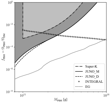
Figure 7: The expected upper limit on the PBH abundance $f_{\rm PBH}\equiv\Omega_{\rm PBH}/\Omega_{DM}$ for a given PBH mass from JUNO with an effective running time of 10 years and a fiducial LS mass of $20$ kton. The solid and dashed curves stand for the upper limits from JUNO in the case of Majorana and Dirac neutrinos, respectively. The dot-dashed curve denotes the upper limit from Super-K Dasgupta et al. (2020). The cruciate-pixels curve is the constraint from the $511$keV $\gamma$-ray line due to $e^{-}$-$e^{+}$ annihilation measured by INTEGRAL Dasgupta et al. (2020). The dotted curve denotes the constraint from the extragalactic $\gamma$-rays (EG) Carr et al. (2009).

V Concluding Remarks

Motivated by the attractive scenario of PBH dark matter, we have calculated the PBH-induced neutrino and antineutrino fluxes due to the Hawking radiation and the corresponding neutrino event spectra at JUNO. The main conclusion is that the current limit on the PBH abundance $f_{\rm PBH}$ from Super-K will be improved by one order of magnitude at JUNO.

One should notice that PBH have been assumed to follow the monochromatic mass distribution and to be spinless. However, there are indeed different theoretical scenarios, in which the predicted mass distribution of PBH is broad Carr (1975); Harada et al. (2016); Kannike et al. (2017); Yokoyama (1998) or the PBH spins are high Harada et al. (2017); Arbey et al. (2020). For the PBH with a log-normal mass distribution, the shaded regions in Fig. 7 would be shallower but broader (e.g., see Fig. 2 in Ref. Dasgupta et al. (2020)). For the spinning PBH, the constraints would be more stringent because of more intense Hawking radiation Macgibbon and Webber (1990); Macgibbon (1991). Therefore, the exclusion limits obtained in the present work can be regarded to be conservative. Our approach can be easily generalized to study more generic scenarios of PBH, which is however beyond the scope of this paper.

As shown in Eq. (4), a different choice of the density profile of dark halo may affect the neutrino fluxes from the Galaxy. Besides the NFW profile, we have also considered two other typical scenarios, i.e., the ISO profile and the EIN profile Ng et al. (2014). Define the relative error as

$$\mathrm{err}(\mathrm{X})\equiv\frac{|{\rm d}F_{\mathrm{Gal}}/{{\rm d}E}(\mathrm{X})-{\rm d}F_{\mathrm{Gal}}/{{\rm d}E}(\mathrm{NFW})|}{{\rm d}F_{\mathrm{Gal}}/{{\rm d}E}(\mathrm{NFW})}\ .$$ (13)

We find that its magnitude is about $1.6\%,0.3\%$ for $\mathrm{X}=\mathrm{\ac{ISO}}$ and EIN, respectively. These errors are small enough for us to safely ignore the uncertainty from different choices of the density profiles. Therefore, we just take the NFW profile in the present work for illustration.

Neutrino flavor conversions may also affect the detection of neutrinos from PBHs at JUNO. Given the neutrino $\nu_{\alpha}$ emitted from the PBHs, the probability to have $\nu_{\beta}$ at the detector is given by Xing and Zhou (2011)

$$\begin{split}P(\alpha\rightarrow\beta)=&\sum_{j=1}^{3}|U_{\alpha j}|^{2}|U_{\beta j}|^{2}\\ &+2\mathrm{Re}\sum_{j<k}U_{\alpha j}U_{\beta k}U_{\alpha k}^{\ast}U_{\beta j}^{\ast}e^{-i\frac{\Delta m_{kj}^{2}}{2E}L}\\ \approx&\sum_{j=1}^{3}|U_{\alpha j}|^{2}|U_{\beta j}|^{2}\ ,\end{split}$$ (14)

where $U_{\alpha j}$ (for $\alpha=e,\mu,\tau$ and $j=1,2,3$) denote the elements of the lepton flavor mixing matrix Maki et al. (1962), $\Delta m^{2}_{kj}\equiv m^{2}_{k}-m^{2}_{j}$ (for $kj=21,31,32$) are neutrino mass-squared differences, $E$ is the neutrino energy, and $L$ is the distance between the neutrino source and the detector. In Eq. (14), the complete decoherence of the neutrino state has been assumed such that the oscillation terms disappear, as the distance $L$ between the source to the detector is much longer than the neutrino oscillation length $L_{\rm osc}\equiv 4\pi E/\Delta m^{2}_{21}\approx 3.3\times 10^{5}~{}{\rm m}$ for $E=10~{}{\rm MeV}$ and $\Delta m^{2}_{21}=7.5\times 10^{-5}~{}{\rm eV}^{2}$. Then, the neutrino flux at the detector is related to the original flux via

$$\frac{{\rm d}F^{\rm d}_{\nu_{\alpha}}}{{\rm d}E}=\sum_{\beta}\frac{{\rm d}F_{\nu_{\beta}}}{{\rm d}E}P(\nu_{\beta}\to\nu_{\alpha})\;,$$ (15)

where the oscillation probability $P(\nu_{\beta}\to\nu_{\alpha})$ has been given in Eq. (14) and it is also applicable to antineutrino oscillations. By taking account of neutrino oscillations, we have numerically checked that the corrections to the event spectra in the IBD and $e$ES channels are below $2.5\%$, which will not significantly affect the constraints shown in Fig. 7. In addition, the $p$ES is induced by neutral-current interactions, so it is insensitive to neutrino oscillations.

Another concern is related to the $p$ES channel for the detection of neutrinos and antineutrinos from PBH. Compared to the IBD channel, a considerable event rate produced from PBH is also expected in this channel. However, we have shown that it is severely contaminated by the backgrounds, which have not been well studied so far. The derived limit from JUNO in Fig. 7 will be further improved if new analysis techniques are developed to effectively get rid of such backgrounds An et al. (2015). This exploration will be left for future works.

References

- Abbott et al. (2016) B. Abbott et al. (LIGO Scientific, Virgo), Phys. Rev. Lett. 116, 061102 (2016), arXiv:1602.03837 [gr-qc] .
- Bird et al. (2016) S. Bird, I. Cholis, J. B. Muñoz, Y. Ali-Haïmoud, M. Kamionkowski, E. D. Kovetz, A. Raccanelli, and A. G. Riess, Phys. Rev. Lett. 116, 201301 (2016), arXiv:1603.00464 [astro-ph.CO] .
- Wang et al. (2018) S. Wang, Y.-F. Wang, Q.-G. Huang, and T. G. F. Li, Phys. Rev. Lett. 120, 191102 (2018), arXiv:1610.08725 [astro-ph.CO] .
- Mandic et al. (2016) V. Mandic, S. Bird, and I. Cholis, Phys. Rev. Lett. 117, 201102 (2016), arXiv:1608.06699 [astro-ph.CO] .
- Clesse and García-Bellido (2017a) S. Clesse and J. García-Bellido, Phys. Dark Univ. 18, 105 (2017a), arXiv:1610.08479 [astro-ph.CO] .
- Raidal et al. (2017) M. Raidal, V. Vaskonen, and H. Veermäe, JCAP 1709, 037 (2017), arXiv:1707.01480 [astro-ph.CO] .
- Cholis (2017) I. Cholis, JCAP 06, 037 (2017), arXiv:1609.03565 [astro-ph.HE] .
- Clesse and García-Bellido (2017b) S. Clesse and J. García-Bellido, Phys. Dark Univ. 15, 142 (2017b), arXiv:1603.05234 [astro-ph.CO] .
- Cai et al. (2019) R.-g. Cai, S. Pi, and M. Sasaki, Phys. Rev. Lett. 122, 201101 (2019), arXiv:1810.11000 [astro-ph.CO] .
- Sasaki et al. (2016) M. Sasaki, T. Suyama, T. Tanaka, and S. Yokoyama, Phys. Rev. Lett. 117, 061101 (2016), [Erratum: Phys.Rev.Lett. 121, 059901 (2018)], arXiv:1603.08338 [astro-ph.CO] .
- Ali-Haïmoud et al. (2017) Y. Ali-Haïmoud, E. D. Kovetz, and M. Kamionkowski, Phys. Rev. D96, 123523 (2017), arXiv:1709.06576 [astro-ph.CO] .
- Chen and Huang (2018) Z.-C. Chen and Q.-G. Huang, Astrophys. J. 864, 61 (2018), arXiv:1801.10327 [astro-ph.CO] .
- Hawking (1971) S. Hawking, Mon. Not. Roy. Astron. Soc. 152, 75 (1971).
- Carr and Hawking (1974) B. J. Carr and S. Hawking, Mon. Not. Roy. Astron. Soc. 168, 399 (1974).
- Chapline (1975) G. F. Chapline, Nature 253, 251 (1975).
- Carr et al. (2020) B. Carr, K. Kohri, Y. Sendouda, and J. Yokoyama, (2020), arXiv:2002.12778 [astro-ph.CO] .
- Carr and Kuhnel (2020) B. Carr and F. Kuhnel, (2020), 10.1146/annurev-nucl-050520-125911, arXiv:2006.02838 [astro-ph.CO] .
- Hawking (1975) S. Hawking, Commun. Math. Phys. 43, 199 (1975), [Erratum: Commun.Math.Phys. 46, 206 (1976)].
- Boudaud and Cirelli (2019) M. Boudaud and M. Cirelli, Phys. Rev. Lett. 122, 041104 (2019), arXiv:1807.03075 [astro-ph.HE] .
- Dasgupta et al. (2020) B. Dasgupta, R. Laha, and A. Ray, Phys. Rev. Lett. 125, 101101 (2020), arXiv:1912.01014 [hep-ph] .
- Arbey et al. (2019) A. Arbey, J. Auffinger, and J. Silk, (2019), 10.1103/PhysRevD.101.023010, arXiv:1906.04750 .
- Carr et al. (2009) B. J. Carr, K. Kohri, Y. Sendouda, and J. Yokoyama, (2009), 10.1103/PhysRevD.81.104019, arXiv:0912.5297 .
- Laha (2019) R. Laha, Phys. Rev. Lett. 123, 251101 (2019), arXiv:1906.09994 [astro-ph.HE] .
- Laha et al. (2020) R. Laha, J. B. Muñoz, and T. R. Slatyer, Phys. Rev. D 101, 123514 (2020), arXiv:2004.00627 [astro-ph.CO] .
- Ballesteros et al. (2020) G. Ballesteros, J. Coronado-Blázquez, and D. Gaggero, Phys. Lett. B 808, 135624 (2020), arXiv:1906.10113 [astro-ph.CO] .
- Lunardini and Perez-Gonzalez (2020) C. Lunardini and Y. F. Perez-Gonzalez, JCAP 08, 014 (2020), arXiv:1910.07864 [hep-ph] .
- Page (1976) D. N. Page, Physical Review D 13, 198 (1976).
- Macgibbon and Webber (1990) J. H. Macgibbon and B. R. Webber, Phys Rev D Part Fields 41, 3052 (1990).
- Macgibbon (1991) J. H. Macgibbon, Phys Rev D Part Fields 44, 376 (1991).
- Siegert et al. (2016) T. Siegert, R. Diehl, A. C. Vincent, F. Guglielmetti, M. G. Krause, and C. Boehm, Astron. Astrophys. 595, A25 (2016), arXiv:1608.00393 [astro-ph.HE] .
- Ackermann et al. (2015) M. Ackermann et al. (Fermi-LAT), Astrophys. J. 799, 86 (2015), arXiv:1410.3696 [astro-ph.HE] .
- Bays (2012) K. Bays (Super-Kamiokande), J. Phys. Conf. Ser. 375, 042037 (2012).
- An et al. (2015) F. An, G. An, Q. An, V. Antonelli, et al., (2015), 10.1088/0954-3899/43/3/030401, arXiv:1507.05613 .
- Arbey and Auffinger (2019) A. Arbey and J. Auffinger, The European Physical Journal C 79, 693 (2019).
- Chiba and Yokoyama (2017) T. Chiba and S. Yokoyama, Progress of Theoretical and Experimental Physics 2017 (2017), 10.1093/ptep/ptx087.
- Mirbabayi et al. (2020) M. Mirbabayi, A. Gruzinov, and J. Noreña, JCAP 03, 017 (2020), arXiv:1901.05963 [astro-ph.CO] .
- Aghanim et al. (2018) N. Aghanim et al. (Planck), (2018), arXiv:1807.06209 [astro-ph.CO] .
- Ng et al. (2014) K. C. Ng, R. Laha, S. Campbell, S. Horiuchi, B. Dasgupta, K. Murase, and J. F. Beacom, Physical Review D 89, 083001 (2014).
- Li et al. (2017) H.-L. Li, Y.-F. Li, M. Wang, L.-J. Wen, and S. Zhou, (2017), 10.1103/PhysRevD.97.063014, arXiv:1712.06985 .
- Strumia and Vissani (2003) A. Strumia and F. Vissani, Phys. Lett. B 564, 42 (2003), arXiv:astro-ph/0302055 .
- Li et al. (2020) H.-L. Li, Y.-F. Li, L.-J. Wen, and S. Zhou, JCAP 05, 049 (2020), arXiv:2003.03982 [astro-ph.HE] .
- Gando et al. (2012) A. Gando et al. (KamLAND), Astrophys. J. 745, 193 (2012), arXiv:1105.3516 [astro-ph.HE] .
- Möllenberg et al. (2015) R. Möllenberg, F. von Feilitzsch, D. Hellgartner, L. Oberauer, M. Tippmann, V. Zimmer, J. Winter, and M. Wurm, Phys. Rev. D 91, 032005 (2015), arXiv:1409.2240 [astro-ph.IM] .
- Beacom et al. (2002) J. F. Beacom, W. M. Farr, and P. Vogel, Phys. Rev. D 66, 033001 (2002), arXiv:hep-ph/0205220 .
- Jia et al. (2019) J. Jia, Y. Wang, and S. Zhou, Chin. Phys. C 43, 095102 (2019), arXiv:1709.09453 [hep-ph] .
- Fukugita et al. (1988) M. Fukugita, Y. Kohyama, and K. Kubodera, Phys. Lett. B 212, 139 (1988).
- Carr (1975) B. J. Carr, Astrophys. J. 201, 1 (1975).
- Harada et al. (2016) T. Harada, C.-M. Yoo, K. Kohri, K.-i. Nakao, and S. Jhingan, Astrophys. J. 833, 61 (2016), arXiv:1609.01588 [astro-ph.CO] .
- Kannike et al. (2017) K. Kannike, L. Marzola, M. Raidal, and H. Veermäe, JCAP 09, 020 (2017), arXiv:1705.06225 [astro-ph.CO] .
- Yokoyama (1998) J. Yokoyama, Phys. Rev. D 58, 107502 (1998), arXiv:gr-qc/9804041 .
- Harada et al. (2017) T. Harada, C.-M. Yoo, K. Kohri, and K.-I. Nakao, Phys. Rev. D 96, 083517 (2017), [Erratum: Phys.Rev.D 99, 069904 (2019)], arXiv:1707.03595 [gr-qc] .
- Arbey et al. (2020) A. Arbey, J. Auffinger, and J. Silk, Mon. Not. Roy. Astron. Soc. 494, 1257 (2020), arXiv:1906.04196 [astro-ph.CO] .
- Xing and Zhou (2011) Z.-Z. Xing and S. Zhou, Neutrinos in Particle Physics, Astronomy and Cosmology (Zhejiang University Press, 2011).
- Maki et al. (1962) Z. Maki, M. Nakagawa, and S. Sakata, Prog. Theor. Phys. 28, 870 (1962).