Deep Hurdle Networks for Zero-Inflated Multi-Target Regression:
Application to Multiple Species Abundance Estimation

Abstract

A key problem in computational sustainability is to understand the distribution of species across landscapes over time. This question gives rise to challenging large-scale prediction problems since (i) hundreds of species have to be simultaneously modeled and (ii) the survey data are usually inflated with zeros due to the absence of species for a large number of sites. The problem of tackling both issues simultaneously, which we refer to as the zero-inflated multi-target regression problem, has not been addressed by previous methods in statistics and machine learning. In this paper, we propose a novel deep model for the zero-inflated multi-target regression problem. To this end, we first model the joint distribution of multiple response variables as a multivariate probit model and then couple the positive outcomes with a multivariate log-normal distribution. By penalizing the difference between the two distributions’ covariance matrices, a link between both distributions is established. The whole model is cast as an end-to-end learning framework and we provide an efficient learning algorithm for our model that can be fully implemented on GPUs. We show that our model outperforms the existing state-of-the-art baselines on two challenging real-world species distribution datasets concerning bird and fish populations.

1 Introduction

Since the Industrial Revolution there has been an increase in biodiversity loss, due to a combination of factors such as agriculture, urbanization, and deforestation, as well as climate change and human introduction of non-native species to ecosystems. Biodiversity loss is a great challenge for humanity, given the importance of biodiversity for sustaining ecosystem services. For example, bird species play a key role in regulating ecosystems by controlling pests, pollinating flowers, spreading seeds and regenerating forests. In a current study it was shown that the bird population in the United States and Canada has fallen by an estimated $29\%$ since 1970 Rosenberg et al. (2019). The biomass of top marine predators has declined substantially in many cases, McCauley et al. (2015), and many marine species are shifting rapidly to new regions in response to changing ocean conditions Pinsky et al. (2020). More generally, a recent report from the United Nations warned that about a million animal and plant species face extinction  Brondizio et al. (2019).

To protect and conserve species, a key question in computational sustainability concerns understanding the distribution of species across landscapes over time, which gives rise to challenging large-scale spatial and temporal modeling and prediction problems Gomes et al. (2019). In particular, ecologists are interested in understanding how species interact with the environment as well as how species interact with each other. Joint species distribution modeling is therefore a computational challenge, as we are interested in simultaneously modeling the correlated distributions of potentially hundreds of species, rather than a single species at a time as traditionally done. Another challenge in joint species distribution modeling is that often outcomes of interest, such as local species abundance in terms of counts or biomass, are sparsely observed, leading to zero-inflated data Morley et al. (2018). Zero-inflated data are frequent in many other settings beyond ecology, for example in research studies concerning public health when counting the number of vaccine adverse events Rose et al. (2006) and prediction of sparse user-item consumption rates Lichman and Smyth (2018).

Herein we propose general models for jointly estimating counts or abundance for multiple entities, which are referred to as zero-inflated multi-target regression. While our models are general, we focus on computational sustainability applications, in particular the joint estimation of counts of multiple bird species and biomass of multiple fish species. As discussed above, many of these species have suffered dramatic reductions or changes in geographic distributions in recent years.

Our contributions are:

1. We propose a deep generalization of the conventional model for multi-target regression that simultaneously models zero-inflated data and the correlations among the multiple response variables.

2. We provide an efficient end-to-end learning framework for our model that can be implemented on GPUs.

3. We evaluate our model as well as state-of-the art joint distribution models on two datasets from computational sustainability that concern the distributions of fish and bird species.

2 Related Work

A popular model for zero-inflated data is the so-called hurdle model Mullahy (1986) in which a Bernoulli distribution governs the binary outcome of whether a response variable has a zero or positive realization; if the realization is positive, the “hurdle” is crossed, and the conditional distribution of the positives is governed by a zero-truncated parametric distribution. Although the hurdle model is popular for zero-inflated data, it has several limitations: 1) the two components of the model are assumed to be independent; 2) it does not explicitly capture the relationships between multiple response variables; and 3) its traditional implementation does not scale. In our work, we address these three key limitations.

A closely related alternative to handle zero-inflated count data is the family of zero-inflated models Lichman and Smyth (2018), in which the response variable is also modeled as a mixture of a Bernoulli distribution and a parametric distribution on non-negative integers such as the Poisson or negative binomial distributions. Different from hurdle model, the conditional distribution of a zero-inflated model is not required to be zero-truncated. In other words, while the hurdle model assumes zeros only come from the Bernoulli distribution, a zero-inflated model assumes zeros could come from both the Bernoulli distribution and the conditional distribution. To account for the inherent correlation of response variables, a class of multi-level zero-inflated regression models was presented Almasi et al. (2016). With such a model, response variables are organized in a hierarchical structure. Response variables are taken to be independent between clusters. Cluster level and within-cluster correlations of response variables are modeled explicitly through random effects attached to linear predictors. However, characterising a suitable hierarchical structure is nontrivial, and these models also do not explicitly capture covariance relations between response variables.

The general problem of multiple-target regression has been extensively studied Borchani et al. (2015); Xi et al. (2018); Xu et al. (2019). Existing methods for multi-output regression can be categorized as: (1) problem transformation methods that transform the multi-output problem into independent single-output problems each solved using a single-output regression algorithm, such as multi-target regressor stacking (MTRS) Spyromitros-Xioufis et al. (2016) and regressor chains (RC) Melki et al. (2017); and (2) algorithm adaptation methods that adapt a specific single-output method to directly handle multi-output dataset, such as multi-objective random forest (MORF) Kocev et al. (2007), random linear target combination (RLTC) Tsoumakas et al. (2014), and multi-output support vector regression (MOSVR) Zhu and Gao (2018). An empirical comparison of three representative state-of-the-art multi-output regression learning algorithms, MTRS, RLTC and MORF, is presented in Xi et al. (2018). Although these advanced multiple-output regression algorithms exploit some correlation between response variables to improve predictive performance, they do not fully model the covariance structure of the response variables and do not consider zero-inflated data. Our work explicitly models zero-inflated data in multi-target regression and it also explicitly models the covariance underlying the phenomena to better characterize the correlation among entities.

3 Preliminaries

In this section we give a brief introduction to the hurdle model and multivariate probit model. In the following we use $\mathbb{R}$, $\mathbb{R}_{0}$, $\mathbb{R}_{+}$, $\mathbb{N}$, $\mathbb{N}_{0}$ and $\mathbb{N}_{+}$ to denote the reals, nonnegative reals, positive reals, integers, nonnegative integers and positive integers, respectively. If an $L$-dimensional vector $y$ is integral, we write $y\in\mathbb{N}^{L}$. We write $y\in\mathbb{R}^{L}$ if $y$ is real. Two vectors $x,y\in\mathbb{R}^{L}$ satisfy $x\preccurlyeq y$ (or $x\succcurlyeq y$) iff $x_{j}\leq y_{j}$ (or $x_{j}\geq y_{j}$) for $1\leq j\leq L$. Since we consider the problem of species abundance estimation, in the following all label data are assumed to be nonnegative. We denote the probability density function (PDF) and the cumulative density function (CDF) of a multivariate normal distribution $\mathcal{N}(\mu,\Sigma)$ as $\phi(x\nonscript\>|\nonscript\>\mathopen{}\allowbreak\mu,\Sigma)$ and $\Phi(x\nonscript\>|\nonscript\>\mathopen{}\allowbreak\mu,\Sigma)$, respectively.

3.1 Hurdle Model

The hurdle model aims to fit data with two independent distributions: (1) a Bernoulli distribution which governs the binary outcome of a response variable being zero or positive; and (2) a zero-truncated distribution of the positive response variable. Specifically, given a dataset $D=\{(x,y)^{(i)}\nonscript\>|\nonscript\>\mathopen{}\allowbreak i=1,\ldots,N\}$, where $x\in\mathbb{R}^{M}$ is the feature data and $y\in\mathbb{R}^{L}_{0}$ (or $y\in\mathbb{N}_{0}^{L}$) is the label data, and let $p_{j}$ be the probability of $y_{j}$ $(1\leq j\leq L)$ being positive, then we have $y_{j}^{\prime}\sim\text{Bernoulli}(p_{j})$, where $y_{j}^{\prime}=1$ if $y_{j}>0$ and $0$ otherwise. Let $f(y_{j}\nonscript\>|\nonscript\>\mathopen{}\allowbreak y_{j}>0)$ be the PDF of the zero-truncated distribution of $y_{j}$. The likelihood of $y_{j}$ is given as $\mathcal{L}(y_{j})=\Pr(y_{j}^{\prime}{\color[rgb]{0,0,0}=1})f(y_{j}\nonscript\>|\nonscript\>\mathopen{}\allowbreak y_{j}>0)$.

3.2 Multivariate Probit Model

Given a dataset $D=\{(x,y^{\prime})^{(i)}\nonscript\>|\nonscript\>\mathopen{}\allowbreak i=1,\ldots,N\}$, where $x\in\mathbb{R}^{M}$ is the feature data and $y^{\prime}\in\{0,1\}^{L}$ is the present/absent label data, the multivariate probit model (MVP) Chen et al. (2018) maps the Bernoulli distribution of each binary response variable $y_{j}^{\prime}$ to a latent variable $r_{j}\in\mathbb{R}$ through threshold $0$, where $r=(r_{1},\ldots,r_{L})$ is subject to a multivariate normal distribution:

$$\Pr(y_{j}^{\prime}=1\nonscript\>|\nonscript\>\mathopen{}\allowbreak x) =\Pr(r_{j}>0\nonscript\>|\nonscript\>\mathopen{}\allowbreak x)$$ (1)

$$\Pr(y_{j}^{\prime}=0\nonscript\>|\nonscript\>\mathopen{}\allowbreak x) =\Pr(r_{j}\leq 0\nonscript\>|\nonscript\>\mathopen{}\allowbreak x)$$ (2)

where $r\sim\mathcal{N}(\mu,\Sigma)$. The joint likelihood of $y^{\prime}$ is given as

$$\mathcal{L}(y^{\prime}\nonscript\>|\nonscript\>\mathopen{}\allowbreak x)=\int_{A_{1}}\cdots\int_{A_{L}}\phi(r\nonscript\>|\nonscript\>\mathopen{}\allowbreak\mu,\Sigma)\text{ d}r_{1},\cdots,\text{d}r_{L}$$ (3)

where $A_{j}=(-\infty,0]$ if $y_{j}^{\prime}=0$, $A_{j}=[0,\infty)$ if $y_{j}^{\prime}=1$. Although there is no closed-form expression for the CDF of a general multivariate normal distribution, Chen et al. (2018) proposed an efficient parallel sampling algorithm to approximate it. We can first translate equation (3) into the CDF of a multivariate normal distribution using the affine transformation:

$$\mathcal{L}(y^{\prime}\nonscript\>|\nonscript\>\mathopen{}\allowbreak x)=\Phi(0\nonscript\>|\nonscript\>\mathopen{}\allowbreak-\mu^{\prime},\Sigma^{\prime})$$ (4)

where $\mu^{\prime}=U\mu$, $\Sigma^{\prime}=U\Sigma U$, and $U=\mbox{diag}(2y^{\prime}-1)\in\{-1,0,1\}^{L\times L}$ is the diagonal matrix with vector $2y^{\prime}-1$ as its diagonal. By decomposing $\Sigma^{\prime}$ into $I+\Sigma^{\prime\prime}$, where $I$ is the identity matrix, a random variable $r\sim\mathcal{N}(0,\Sigma^{\prime})$ can be written as $r=z-w$, where $z\sim\mathcal{N}(0,I)$ and $w\sim\mathcal{N}(0,\Sigma^{\prime\prime})$. Then, $\Phi(0\nonscript\>|\nonscript\>\mathopen{}\allowbreak-\mu^{\prime},\Sigma^{\prime})$ can be approximated as

lCl Φ( 0  —  -μ’, Σ’ ) &= Pr(r-μ’ ≼0) = Pr(z-w ≼μ’)
3l= E_w∼N(0, Σ”) [Pr( z ≼(w+μ’) —  w )]
3l= E_w∼N(μ’, Σ”) [∏_j=1^L Φ(w_j)]
3l ≈1K∑_k=1^K ∏_j=1^L Φ(w_j^(k)) where samples $\{w^{(k)}\}$ are subject to $\mathcal{N}(\mu^{\prime},\Sigma^{\prime\prime})$ and $\Phi$ is the CDF of the standard normal distribution. Note that according to (4), we have $\Sigma^{\prime\prime}=\Sigma^{\prime}-I=U\Sigma U-I=U(\Sigma-I)U$.

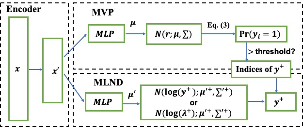
Figure 1: The deep hurdle network architecture. An encoder is used to learn latent features $x^{\prime}$, an MVP is used to model the joint distribution of multiple response variables $y$ being zero or positive, and an MLND is used to model the joint distribution of positive response variables $y^{+}$. The MVP and MLND are linked by sharing the same latent features $x^{\prime}$, and penalizing the difference between their covariance matrices $\Sigma$ and $\Sigma^{\prime}$.

4 Deep Hurdle Network

In this paper we provide a deep generalization of the hurdle model, within an autoencoder framework, which we call the deep hurdle network (DHN). The DHN integrates the MVP to model the joint distribution of multiple response variables being zero or positive, and the multivariate log-normal distribution (MLND) to model the positive response variables. The MVP and MLND share the same latent features, and differences between their covariance matrices are penalized. Specifically, given a dataset $D=\{(x,y)^{(i)}\nonscript\>|\nonscript\>\mathopen{}\allowbreak i=1,\ldots,N\}$, where $x\in\mathbb{R}^{M}$ is the feature data and $y\in\mathbb{R}^{L}_{0}$ (or $y\in\mathbb{N}_{0}^{L}$) is the label data, the hurdle network contains three parts (see Figure 1 for an illustration):

• Encoder: An encoder maps the raw features $x\in\mathbb{R}^{M}$ to latent features $x^{\prime}\in\mathbb{R}^{{\color[rgb]{0,0,0}M^{\prime}}}$.

• MVP: Label data $y\in\mathbb{R}^{L}_{0}/\mathbb{N}^{L}_{0}$ are translated into binary label data $y^{\prime}\in\{0,1\}^{L}$, where $y^{\prime}=(y_{1}^{\prime},\ldots,y_{L}^{\prime})$ and $y_{j}^{\prime}$ equals to $1$ if $y_{j}>0$ and $0$ otherwise. We then use MVP to map $y^{\prime}$ to latent variable $r\in\mathbb{R}^{L}$ via equations (1)–(2), where $r$ is assumed to follow $\mathcal{N}(\mu,\Sigma)$. A multilayer perceptron (MLP) is then used to model $\mu$ given $x^{\prime}$ as input. $\Sigma$ is a global parameter which is learned from random initialization and shared by all data points.

• MLND: Let $y^{+}\in\mathbb{R}_{+}^{P}$ $(P\leq L)$ be the positive part of $y\in\mathbb{R}^{L}$ , where $P$ is the number of positive elements of $y$. $\log(y^{+})=(\log(y_{1}^{+}),\ldots,\log(y_{P}^{+}))$ is directly modeled as a multivariate normal distribution, and $y^{+}$ are assumed to follow a multivariate log-normal distribution. Therefore, we have

  $$\begin{split}\mathcal{L}(\log(y^{+})\nonscript\>|\nonscript\>\mathopen{}\allowbreak x^{\prime})=\phi(\log(y^{+})\nonscript\>|\nonscript\>\mathopen{}\allowbreak{\mu^{\prime}}^{+},{{\color[rgb]{0,0,0}\Sigma^{\prime}}}^{+})\end{split}$$ (5)

  where ${\mu^{\prime}}^{+}$ and ${\Sigma^{\prime}}^{+}$ are the sub-parts of $\mu^{\prime}\in\mathbb{R}^{L}$ and $\Sigma^{\prime}$ that correspond to $y^{+}$ respectively. Note that here $\Sigma^{\prime}$ is encouraged to be similar to the convariance matrix $\Sigma$ of the MVP and $\mu^{\prime}\in\mathbb{R}^{L}$ is modeled with an MLP.
  

  On the other hand, let $y^{+}\in\mathbb{N}^{P}_{+}(P\leq L)$ be the positive part of $y\in\mathbb{N}^{L}$. Each $y_{j}^{+}$ is assumed to follow an univariate Poisson distribution $\Pr(y^{+}_{j}\nonscript\>|\nonscript\>\mathopen{}\allowbreak\lambda_{j}^{+})$ for $1\leq j\leq P$, where $\lambda_{j}^{+}$ is the mean, and $\log(\lambda^{+})=(\log(\lambda_{1}^{+}),\ldots,\log(\lambda_{P}^{+}))$ is assumed to follow a multivariate normal distribution. Therefore, we have

  $$\begin{split}\mathcal{L}(\log({\lambda}^{+})\nonscript\>|\nonscript\>\mathopen{}\allowbreak x^{\prime})=\phi(\log({\lambda}^{+})\nonscript\>|\nonscript\>\mathopen{}\allowbreak{\mu^{\prime}}^{+},{{\color[rgb]{0,0,0}\Sigma^{\prime}}}^{+})\end{split}$$ (6)

There are several advantages of the deep hurdle network over the conventional hurdle model:

• The encoder is forced to learn the salient features and ignore the noise and irrelevant parts of the raw features. This relieves us from selecting which salient features to use in the conventional hurdle model.

• DHN adopts MVP and MLND to handle correlations between multiple response variables explicitly via covariance matrices, which is not considered in the conventional hurdle model.

• The two components of the conventional hurdle model are independent, while in DHN the MVP and MLND are linked by sharing the same latent features, and penalizing the different between their covariance matrices.

4.1 End-to-End Learning for DHN

Parameters of a deep model are usually estimated by minimizing the negative log-likelihood (NLL). We develop two different learning objectives for nonnegative continuous and count data, respectively. After selecting our objective function, we can estimate the parameters of the deep hurdle network by minimizing the objective function via stochastic gradient descent (SGD).

4.1.1 Learning Objective for Nonnegative Continuous Data

If response variables $y$ are nonnegative reals, then we combine equations (4), (3.2) and (5) to obtain the negative log-likelihood (NLL) function: l -log(L( y’ —  x’ )L( log(y^+)  —  x’ ))
= -log(E_w ∼N(Uμ,U(Σ-I) U)[∏_j=1^L Φ(w_j)])
1l=-log(ϕ( log(y^+)  —  μ’^+,Σ’^+ )) The first part of the right-hand side of equation (4.1.1) can be approximated by a set of samples $\{w^{(k)}\}$ from $\mathcal{N}(U\mu,U(\Sigma-I)U)$: $-\log(\frac{1}{K}\sum_{k=1}^{K}\exp(\sum_{j=1}^{L}\log(\Phi(w_{j}^{(k)}))))$. Such a set of samples can be obtained by first using the Cholesky decomposition, which decomposes $\Sigma-I$ into $CC^{T}$, and then generating independent samples $v^{(k)}\sim\mathcal{N}(0,I)$ to yield $w^{(k)}=U(\mu+Cv^{(k)})$. According to the affine transformation of the normal distribution, the samples $\{w^{(k)}\}$ are subject to $\mathcal{N}(U\mu,U(\Sigma-I)U)$. However, doing the matrix multiplications $U\mu$ and $UCv^{(k)}$ are unnecessary since $U=\mbox{diag}(2y^{\prime}-1)\in\{-1,0,1\}^{L\times L}$ is the diagonal matrix with vector $2y^{\prime}-1$ as its diagonal. Let $w^{\prime(k)}=\mu+Cv^{(k)}$ such that $\{w^{\prime(k)}\}$ are subject to $\mathcal{N}(\mu,\Sigma-I)$, then it is easy to show that $\log(\Phi(w_{j}^{(k)}))=y_{j}^{\prime}\log(\Phi(w^{\prime(k)}_{j}))+(1-y_{j}^{\prime})\log(1-\Phi(w^{\prime(k)}_{j}))$. Thus, we can approximate equation (4.1.1) as follows: l - log(1K∑_k=1^Kexp(∑_j=1^L (y_j’log(Φ(w^(k)_j))
1r+ (1-y_j’)log(1-Φ(w^(k)_j)))))
-log(ϕ( log(y^+)  —  μ’^+,Σ’^+ )) where samples $\{w^{(k)}\}$ are subject to $\mathcal{N}(\mu,\Sigma-I)$.

4.1.2 Learning Objective for Count Data

If response variables $y$ are nonnegative integers, let $y^{+}\in\mathbb{N}_{+}^{P}$ be the positive part of $y\in\mathbb{N}_{0}^{L}(P\leq L)$, where $P$ is the number of positive elements of $y$, then each $y_{j}^{+}$ is assumed to follow a univariate Poisson distribution $\Pr(y_{j}^{+};\lambda_{j}^{+})$, and $\log(\lambda^{+})=(\log(\lambda_{1}^{+}),\ldots,\log(\lambda_{P}^{+}))$ is assumed to follow a multivariate normal distribution $\mathcal{N}({\mu^{\prime}}^{+},{\Sigma^{\prime}}^{+})$. The likelihood of response variables $y^{+}$ is given as

$$\begin{split}&\mathcal{L}(y^{+};\lambda^{+}|\mathcal{N}(\log(\lambda^{+});\mu^{\prime},{\Sigma^{\prime}}^{+}),x^{\prime})\\ &=\operatorname*{\mathbb{E}}_{\log(\lambda^{+})\sim\mathcal{N}({\mu^{\prime}}^{+},{\Sigma^{\prime}}^{+})}[\prod_{j=1}^{P}\frac{{\lambda_{j}^{+}}^{y_{j}^{+}}e^{-\lambda_{j}^{+}}}{y_{j}^{+}!}]\end{split}$$ (7)

We then combine equations (4), (3.2) and (7) to obtain the NLL function as follows:

l -log(L(y’—x’)L(y^+;λ^+—N(log(λ^+);μ’,Σ’^+), x’)
= -log(E_w ∼N(Lμ,L(Σ-I) L)[∏_j=1^L Φ(w_j)])
1r- log(E_log(λ^+)∼N(μ’^+,Σ’^+) [∏_j=1^P λj+yj+e-λj+yj+!])
≈- log(1K∑_k=1^K(exp(∑_j=1^L (y_j’log(Φ(w^(k)_j)))
1r+ (1-y_j’)log(1-Φ(w^(k)_j)))))
-log(1K∑_k=1^Kexp(∑_j=1^P (y_j^+log(λ^+)_j^(k) - λ_j^(k)-log(y_j^+!))))
where samples $\{w^{(k)}\}$ and $\{\log(\lambda^{+})^{(k)}\}$ are subject to $\mathcal{N}(\mu,\Sigma-I)$ and $\mathcal{N}({\mu^{\prime}}^{+},{\Sigma^{\prime}}^{+})$, respectively.

Lastly, we add an L1 loss term to equations (4.1.1) and (4.1.2), respectively, to penalize the difference between $\Sigma$ and $\Sigma^{\prime}$.

5 Experiments

In this section, we compare our model with the existing state-of-the-art baselines on two challenging real-world species distribution datasets concerning bird and fish populations.

5.1 Datasets

Sea bottom trawl surveys (SBTSs) are scientific surveys that collect data on the distribution and abundance of marine fishes. In each haul (sample), all catches of each species were weighted and recorded, as well as the time, location, sea surface temperature and depth. For each haul, we have additional environmental features from the Simple Ocean Data Assimilation (SODA) Dataset Carton et al. (2018) and Global Bathymetry and Elevation Dataset , such as sea bottom temperature, rugosity, etc. Thus, we have a 17-dimensional feature vector for each haul. We study fish species abundance in the continental shelf around North America and consider SBTSs that were conducted from 1963 to 2015 Morley et al. (2018). We consider the top 100 most frequently observed species as the target species and there are $135,458$ hauls that caught at least one of these species. Among the $135,458*100$ data entries, only $8.5\%$ of them are nonzero. The distribution of the positive data is visualized in Figure 2.

eBird is a crowd-sourced bird observation dataset Munson et al. (2012). A record in this dataset corresponds to a checklist that an experienced bird observer uses to mark the number of birds of each species detected, as well as the time and location. Additionally, we obtain a 16-dimensional feature vector for each observation location from the National Land Cover Dataset (NLCD) Homer et al. (2015) which describes the landscape composition with respect to 16 different land types such as water, forest, etc. We use all the bird observation checklists in North America in the last two weeks of May from 2002 to 2014. We consider the top 100 most frequently observed species as the target species and there are $39,668$ observations that contain at least one of these 100 species. Only $19.8\%$ of these $39,668*100$ data entries are nonzero. The distribution of the positive data is visualized in Figure 2.

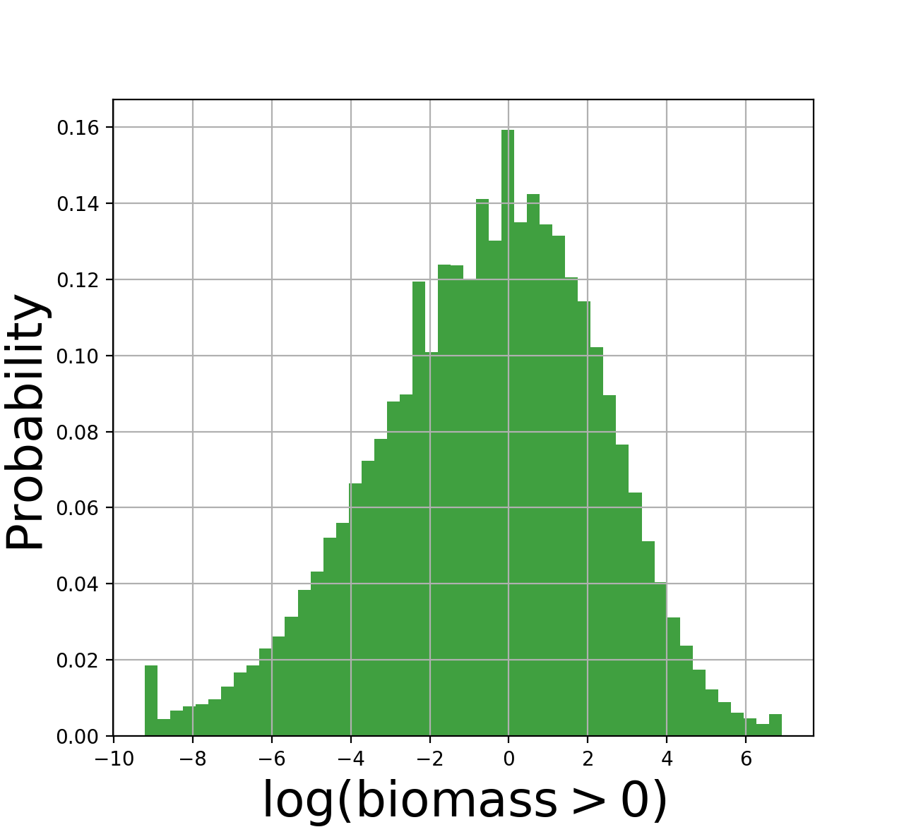
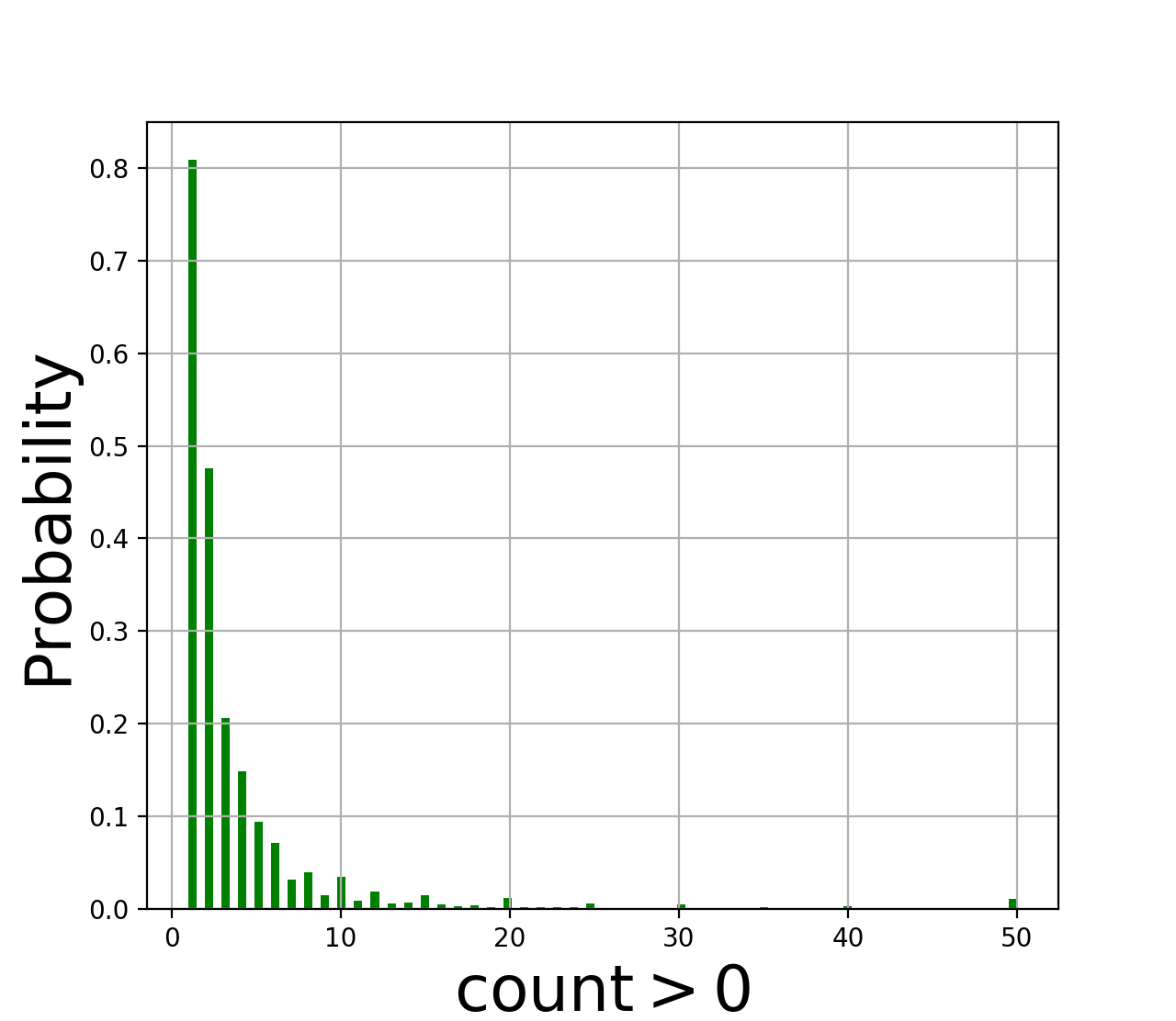
Figure 2: Visualization of data distribution. The left figure shows that the sea bottom trawl survey data approximately follow a log-normal distribution, and the right figure shows that the eBird data approximately follow a Poission distribution.

5.2 Evaluation Metrics

For the task of multi-target regression, we employ and adapt two well known measures: the average correlation coefficient (ACC)and root mean squared error (RMSE) Borchani et al. (2015); Xu et al. (2019). The ACC is defined as:

$$\frac{1}{L}\sum_{j=1}^{L}\frac{\sum_{i=1}^{N_{\text{test}}}(y_{j}^{(i)}-\bar{y}_{j})(\hat{y}_{j}^{(i)}-\bar{\hat{y}}_{j})}{\sqrt{\sum_{i=1}^{N_{\text{test}}}(y_{j}^{(i)}-\bar{y}_{j})^{2}\sum_{i=1}^{N_{\text{test}}}(\hat{y}_{j}^{(i)}-\hat{\bar{y}}_{j})^{2}}},$$

where $L$ is the number of response variables, $N_{\text{test}}$ is the number of testing samples, $y^{(i)}$ and $\hat{y}^{(i)}$ are the vectors of the actual and predicted outputs for $x^{(i)}$, respectively, and $\bar{y}$ and $\bar{\hat{y}}$ are the vectors of averages of the actual and predicted outputs, respectively. Since the data considered here are zero-inflated, using standard RMSE might not be appropriate. Models can produce degenerate results by simply predicting a near-zero vector for each test data point. Therefore, we adapt the RMSE to the zero-inflated setting by considering zero and positive parts of the output separately. Let $y^{(i)}$ be the actual $L$-dimensional output vector of the $i$-th testing point, $I_{0}$ (respectively, $I_{+}$) be the set of indices of zero (respectively, positive) elements in $y^{(i)}$, and $\hat{y}$ be the predicted $L$-dimensional output vector, then we define the zero-inflated RMSE (zRMSE) as:

$$\frac{\sum_{i=0}^{N_{\text{test}}}\sqrt{\frac{\alpha\sum_{j\in I_{0}}(\hat{y}^{(i)}_{j})^{2}}{|I_{0}|}+\frac{(1-\alpha)\sum_{j\in I_{+}}(y^{(i)}_{j}-\hat{y}^{(i)}_{j})^{2}}{|I_{+}|}}}{N_{\text{test}}},$$

where $0\leq\alpha\leq 1$ is the relative importance of the zero part.

From the above new definition, we can see that the zero and positive parts of an output are both considered, therefore, a model cannot cheat by predicting near-zero vectors by ignoring the positive parts of the outputs. Finally, we also compare the time to learn different models.

5.3 Baselines

We consider both the state-of-the-art hurdle/zero-inflated models in statistics and multi-target regression models in machine learning:

1) Hurdle/zero-inflated models. For the bird counting data, we select the state-of-the-art multi-level zero-inflated Poisson model (MLZIP) Almasi et al. (2016) as a baseline. For the fish biomass data, we modify the MLZIP by replacing the Poisson with log-normal, which we denote as multi-level zero-inflated log-normal (MLZILN) model, as a baseline. For both the baselines, response variables are divided into random clusters.

2) Multi-target regression models. As we have discussed in Section 2, there are two kinds of methods for multi-target regression models: for problem transformation methods, we select the state-of-the-art multi-target regressor stacking (MTRS) Spyromitros-Xioufis et al. (2016) as a baseline; and, for algorithm adaptation methods, we select the state-of-the-art multi-objective random forest (MORF) Kocev et al. (2007), random linear target combination (RLTC) Tsoumakas et al. (2014), multi-output support vector regression (MOSVR) Zhu and Gao (2018), and multi-layer multi-target regression (MMR) Zhen et al. (2017) as baselines.

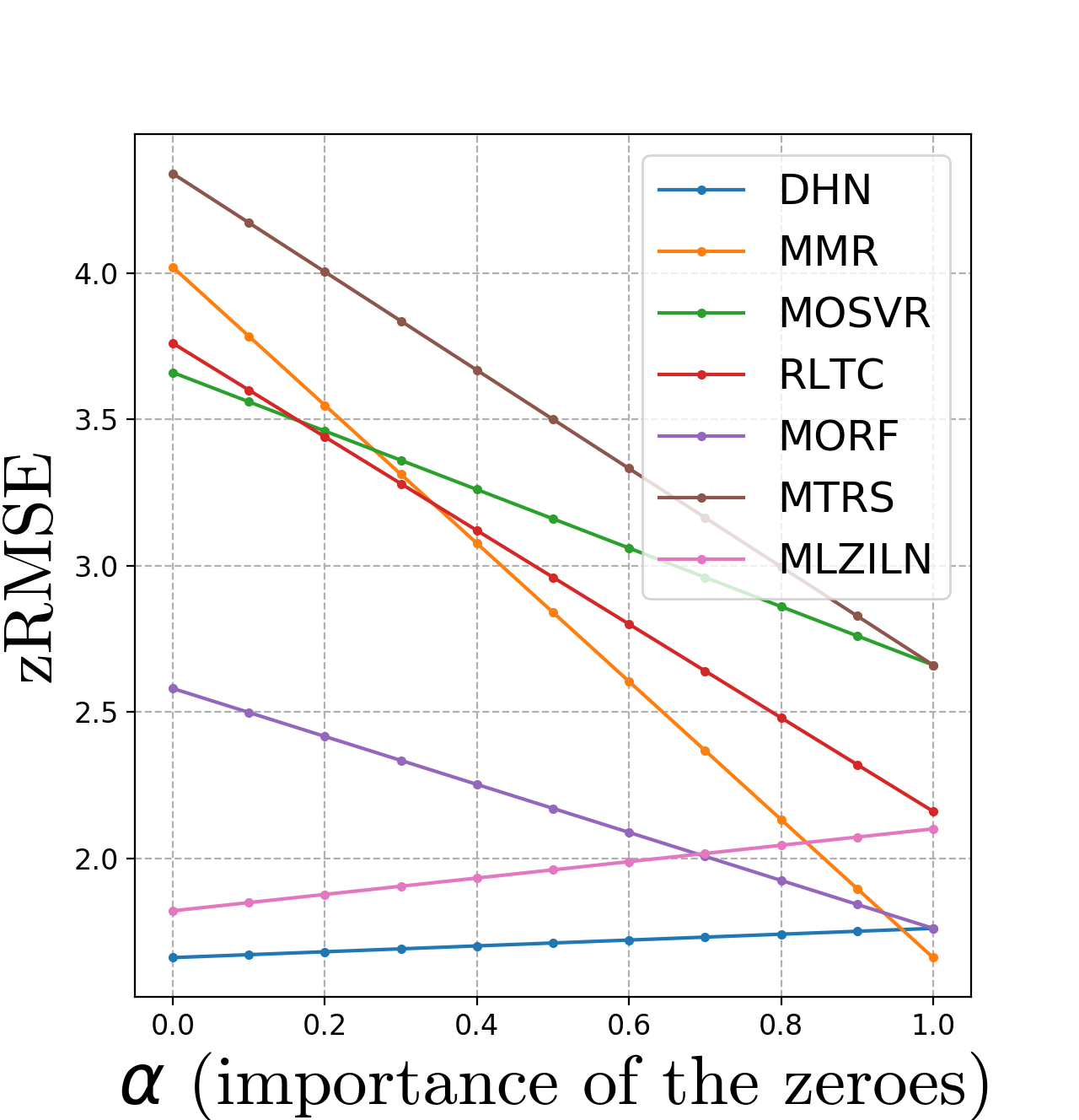
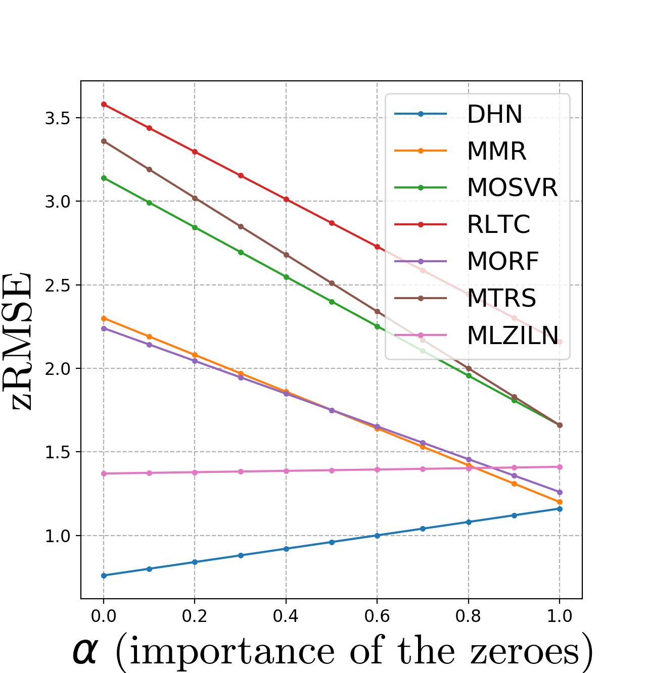
Figure 3: zRMSE of the methods with different $\alpha$ ratios on the SBTS (left) and eBird (right) datasets.

5.4 Implementations and Results

Metrics	MLZILN	MTRS	MORF	RLTC	MOSVR	MMR	DHN
ACC	0.52	0.31	0.45	0.40	0.32	0.47	0.65
zRMSE	1.96	3.50	2.17	2.96	3.16	2.84	1.71
Time (min)	218	76	87	96	120	55	57

Metrics	MLZIP	MTRS	MORF	RLTC	MOSVR	MMR	DHN
ACC	0.50	0.32	0.41	0.19	0.39	0.27	0.59
zRMSE	1.39	2.51	1.75	2.87	2.40	1.75	0.96
Time (min)	186	56	64	85	99	53	45

Table 1: Performance comparison between selected models on the SBTS (top) and eBird (bottom) datasets. The best scores are in bold. Except for the MLZILN/MLZIP model, each score is the average after 3 runs. $\alpha$ of zRMSE is set to be 0.5.

Our experiments were carried out on a computer with a 4.2 GHz quad-core Intel i7 CPU, 16 GB RAM and an NVIDIA Quadro P4000 GPU card. We use grid search to find the best hyperparameters for all models, e.g. learning rates, learning rate decay ratio, and tree depth. The encoders of DHN are parametrized by 3-layer fully connected neural networks with latent dimensionalities 512 and 256, and the MLPs of MVP and MLND are 2-layer fully connected neural networks with latent dimensionalities 256. The activation functions in neural networks are set to be ReLU. Neural network models are trained with 100 epochs and batches size 128 for the eBird dataset and 256 for the SBTS dataset. We randomly split the two datasets into three parts for training ($70\%$), validating ($15\%$) and testing ($15\%$), respectively.

The results are shown in Table 1. As expected, MLZILN/MLZIP and DHN outperform other multi-target regression models in terms of zRMSE because the former models capture zero-inflation of the datasets. DHN has $12.8\%$ and $30.9\%$ lower errors than MLZILN and MLZIP, respectively. On the other hand, DHN has the best ACC on both datasets, which shows the benefit of employing and sharing the same covariance matrix to capture multi-entities correlations. In terms of model training time, MLZILN and MLZIP are far worse than other machine learning models, while DHN and MMR are the best. We also compare zRMSE of the methods under different $\alpha$ ratios in Figure 3. We can see that zero-inflated models tends to perform better for positive parts, while other nonzero-inflated models tend to underestimate the positive parts.

5.5 Ablation Studies

To learn the contributions of different components in DHN, we perform simple ablation studies. We modify the DHN architecture and rerun the experiments in the following cases:

• We remove the encoder so that both the MVP and MLND directly use the raw features as input.

• We remove both the encoder and the MVP so that only the MLND is used.

• We do not penalize the difference between the covariance matrices of MVP and MLND.

The results are presented in Table 2. From the results of ablation case studies, we can observe that: (1) employing an encoder to learn latent features helps; (2) the model’s performance drops significantly if we do not capture zero inflation of data; and (3) penalizing the difference between the covariance matrices of MVP and MLND helps to capture the ACC among multiple entities and boost the model’s performance.

		SBTS			eBird
Metrics	Case 1	Case 2	Case 3	Case 1	Case 2	Case 3
ACC	0.65	0.50	0.45	0.59	0.47	0.43
zRMSE	1.91	2.60	1.93	1.52	1.95	1.65
Time (min)	55	56	57	44	45	45

Table 2: Ablation studies. The three cases refer to the ways of modifying our models, which is defined in section 5.5. Each score is the average after 3 runs. $\alpha$ of zRMSE is set to be 0.5.

6 Conclusion

To understand the distribution of species across landscapes over time is a key problem in computational sustainability, which gives rise to challenging large-scale prediction problems since hundreds of species have to be simultaneously modeled and the survey data are usually inflated with zeros due to the absence of species for a large number of sites. We refer to this problem of jointly estimating counts or abundance for multiple entities as zero-inflated multi-target regression.

In this paper, we have proposed a novel deep model for zero-inflated multi-target regression, which is called the deep hurdle networks (DHNs). The DHN simultaneously models zero-inflated data and the correlation among the multiple response variables: we first model the joint distribution of multiple response variables as a multivariate probit model and then couple the positive outcomes with a multivariate log-normal distribution. A link between both distributions is established by penalizing the difference between their covariance matrices. We then cast the whole model as an end-to-end learning framework and provide an efficient learning algorithm for our model that can be fully implemented on GPUs. We show that our model outperforms the existing state-of-the-art baselines on two challenging real-world species distribution datasets concerning bird and fish populations. We also performed ablation studies of our models to learn the contributions of different components in the model.

Another related challenging problem in computational sustainability is to forecast how species distribution might be impacted due to the long-term effects of global climate change. In order to tackle the forecast challenge, our future works will consider using recurrent neural networks to improve our model such that it would be able to handle time series data better. On the other hand, we could also borrow ideas of advanced techniques for the multi-label prediction problem to further improve the performance of MVP that is used in our model, e.g. using latent embedding learning to match features and labels in the latent space.

References

- Almasi et al. [2016] Afshin Almasi, Mohammad Reza Eshraghian, Abbas Moghimbeigi, Abbas Rahimi, Kazem Mohammad, and Sadegh Fallahigilan. Multilevel zero-inflated generalized poisson regression modeling for dispersed correlated count data. Statistical Methodology, 30:1–14, 2016.
- Borchani et al. [2015] Hanen Borchani, Gherardo Varando, Concha Bielza, and Pedro Larrañaga. A survey on multi-output regression. Wiley Interdisciplinary Reviews: Data Mining and Knowledge Discovery, 5(5):216–233, 2015.
- Brondizio et al. [2019] Eduardo S. Brondizio, Josef Settele, Sandra Díaz, and Hien T. Ngo. Global assessment report on biodiversity and ecosystem services of the intergovernmental science-policy platform on biodiversity and ecosystem services. IPBES Secretariat, 2019.
- Carton et al. [2018] James A. Carton, Gennady A. Chepurin, and Ligang Chen. Soda3: A new ocean climate reanalysis. Journal of Climate, 31(17):6967–6983, 2018.
- Chen et al. [2018] Di Chen, Yexiang Xue, and Carla Gomes. End-to-end learning for the deep multivariate probit model. In International Conference on Machine Learning, pages 931–940, 2018.
- Gomes et al. [2019] Carla Gomes, Thomas Dietterich, Christopher Barrett, Jon Conrãd, Bistra Dilkina, Stefano Ermon, Fei Fang, And̃rew Farnsworth, Alan Fern, Xiaoli Fern, et al. Computational sustainability: Computing for a better world and a susta inable future. Communications of the ACM, 62(9):56–65, 2019.
- Homer et al. [2015] Collin Homer, Jon Dewitz, Limin Yang, Suming Jin, Patrick Danielson, George Xian, John Coulston, Nathaniel Herold, James Wickham, and Kevin Megown. Completion of the 2011 national land cover database for the conterminous united states–representing a decade of land cover change information. Photogrammetric Engineering & Remote Sensing, 81(5):345–354, 2015.
- Kocev et al. [2007] Dragi Kocev, Celine Vens, Jan Struyf, and Sašo Džeroski. Ensembles of multi-objective decision trees. In European conference on machine learning, pages 624–631, 2007.
- Lichman and Smyth [2018] Moshe Lichman and Padhraic Smyth. Prediction of sparse user-item consumption rates with zero-inflated poisson regression. In Proceedings of the 2018 World Wide Web Conference, pages 719–728, 2018.
- McCauley et al. [2015] Douglas J. McCauley, Malin L. Pinsky, Stephen R. Palumbi, James A. Estes, Francis H. Joyce, and Robert R. Warner. Marine defaunation: animal loss in the global ocean. Science, 347(6219):1255641–1255641, 2015.
- Melki et al. [2017] Gabriella Melki, Alberto Cano, Vojislav Kecman, and Sebastián Ventura. Multi-target support vector regression via correlation regressor chains. Information Sciences, 415:53–69, 2017.
- Morley et al. [2018] James W. Morley, Rebecca L. Selden, Robert J. Latour, Thomas L. Frölicher, Richard J. Seagraves, and Malin L. Pinsky. Projecting shifts in thermal habitat for 686 species on the north american continental shelf. PLOS ONE, 13(5):1–28, 2018.
- Mullahy [1986] John Mullahy. Specification and testing of some modified count data models. Journal of econometrics, 33(3):341–365, 1986.
- Munson et al. [2012] M Arthur Munson, Kevin Webb, Daniel Sheldon, Daniel Fink, Wesley M Hochachka, Marshall Iliff, Mirek Riedewald, Daria Sorokina, Brian Sullivan, Christopher Wood, and Steve Kelling. The ebird reference dataset, version 4.0. Cornell Lab of Ornithology and National Audubon Society, Ithaca, NY, 2012.
- Pinsky et al. [2020] Malin L. Pinsky, Rebecca L. Selden, and Zoë J. Kitchel. Climate-driven shifts in marine species ranges: Scaling from organisms to communities. Annual Review of Marine Science, 12:153–179, 2020.
- Rose et al. [2006] Charles E Rose, Stacey W Martin, Kathleen A Wannemuehler, and Brian D Plikaytis. On the use of zero-inflated and hurdle models for modeling vaccine adverse event count data. Journal of biopharmaceutical statistics, 16(4):463–481, 2006.
- Rosenberg et al. [2019] Kenneth V. Rosenberg, Adriaan M. Dokter, Peter J. Blancher, John R. Sauer, Adam C. Smith, Paul A. Smith, Jessica C. Stanton, Arvind Panjabi, Laura Helft, Michael Parr, and Peter P. Marra. Decline of the north american avifauna. Science, 366(6461):120–124, 2019.
- Spyromitros-Xioufis et al. [2016] Eleftherios Spyromitros-Xioufis, Grigorios Tsoumakas, William Groves, and Ioannis Vlahavas. Multi-target regression via input space expansion: treating targets as inputs. Machine Learning, 104(1):55–98, 2016.
- Tsoumakas et al. [2014] Grigorios Tsoumakas, Eleftherios Spyromitros-Xioufis, Aikaterini Vrekou, and Ioannis Vlahavas. Multi-target regression via random linear target combinations. In Joint european conference on machine learning and knowledge discovery in databases, pages 225–240, 2014.
- Xi et al. [2018] Xuefeng Xi, Victor S Sheng, Binqi Sun, Lei Wang, and Fuyuan Hu. An empirical comparison on multi-target regression learning. Computers, Materials & Continua, 56(2):185–198, 2018.
- Xu et al. [2019] Donna Xu, Yaxin Shi, Ivor W. Tsang, Yew-Soon Ong, Chen Gong, and Xiaobo Shen. A survey on multi-output learning. IEEE Transactions on Neural Networks and Learning Systems, pages 1–21, 2019.
- Zhen et al. [2017] Xiantong Zhen, Mengyang Yu, Xiaofei He, and Shuo Li. Multi-target regression via robust low-rank learning. IEEE transactions on pattern analysis and machine intelligence, 40(2):497–504, 2017.
- Zhu and Gao [2018] Xinqi Zhu and Zhenghong Gao. An efficient gradient-based model selection algorithm for multi-output least-squares support vector regression machines. Pattern Recognition Letters, 111:16–22, 2018.