HAT-P-68b: A Transiting Hot Jupiter Around a K5 Dwarf Star

Abstract

We report the discovery by the ground-based HATNet survey of the transiting exoplanet HAT-P-68b, which has a mass of $0.724\pm 0.043$ $M_{\rm J}$, and radius of $1.072\pm 0.012$ $R_{\rm J}$. The planet is in a circular $P=2.2984$ -day orbit around a moderately bright V = $13.937\pm 0.030$ magnitude K dwarf star of mass $0.673_{-0.014}^{+0.020}$ $M_{\sun}$, and radius $0.6726\pm 0.0069$ $R_{\sun}$. The planetary nature of this system is confirmed through follow-up transit photometry obtained with the FLWO 1.2 m telescope, high-precision RVs measured using Keck-I/HIRES, FLWO 1.5 m/TRES, and OHP 1.9 m/Sophie, and high-spatial-resolution speckle imaging from WIYN 3.5 m/DSSI.

HAT-P-68 is at an ecliptic latitude of $+3^{\circ}$ and outside the field of view of both the NASA TESS primary mission and the K2 mission. The large transit depth of $0.036$ mag ($r$-band) makes HAT-P-68b a promising target for atmospheric characterization via transmission spectroscopy.

1 Introduction

The first detection of a planet orbiting a star besides our own (Mayor & Queloz, 1995) sparked a new era of astronomy and planetary science, and made the discovery and characterization of extra-solar planets a focal point of observational research in astrophysics. Among the various methods available, transit photometry has produced the largest yield of exoplanets to date, and has also proven to be the most sensitive method for discovering small planets. Additionally, transiting exoplanets (TEPs) offer the unique opportunity to study the physical properties of planets outside the Solar System, and how these properties depend on those of their parent stars. Combining transit time-series data with measurements of the radial velocity (RV) orbital wobble of the host star provides the masses and radii of planetary objects – that is, if the stellar mass and radius can be determined through other means. Furthermore, follow-up observations of these systems allow us to study the structure and composition of the planetary atmospheres through transmission spectroscopy (e.g. Charbonneau et al., 2002), and to measure the orbital eccentricity and obliquity (e.g. Morton & Winn, 2014). These capabilities make TEPs one of the most reliable sources for testing current models of planetary formation and evolution.

Many wide-field ground-based surveys have been productive in detecting TEPs, with the largest yields coming from WASP (Pollacco et al., 2006), HATSouth (Bakos et al., 2013) and HATNet (Bakos et al., 2004). The sample of exoplanets discovered by these surveys is highly biased towards giant planets at short orbital distances to their host stars (e.g. Gaudi et al., 2005). These hot Jupiters (HJs) initially shattered our understanding of planetary formation. Space surveys like the all-sky Transiting Exoplanet Survey Satellite (TESS; Ricker et al., 2014) – joining the legacy of Kepler (Borucki et al., 2010), K2 (Howell et al., 2014), and CoRot (Auvergne et al., 2009) – are better equipped to identify objects with a wider range of sizes at a wide range of orbital distances to their host stars (e.g., Nielsen et al., 2020).

Yet, discoveries of planets with orbital periods shorter than 10 days provide advantages to resolving current theoretical challenges in the field (see Dawson & Johnson, 2018). For instance, explaining the inflated radii of HJs remains a theoretical puzzle (e.g. Sestovic et al., 2018, and references therein) that may be elucidated by building up a larger sample objects to disentangle the effects of age, orbital separation, irradiation, composition and mass on the radii of these planets (e.g., Hartman et al., 2016). Explaining the origin of these planets as well as understanding how they evolve via planet-star interactions are subjects that can be better addressed with a larger sample of objects.

The HATNet survey searches for planets transiting moderately bright stars by utilizing six small telephoto lenses on robotic mounts. Specifically, HATNet has two stations with multiple 11 cm telescopes; one of which is located at the Smithsonian Astrophysical Observatory’s Fred Lawrence Whipple Observatory (FLWO) in Arizona, while the other is atop the Mauna Kea Observatory (MKO) in Hawaii. Bakos (2018) provides a recent review of the HATNet and HATSouth projects.

Here we present the discovery by the HATNet survey of a transiting, short-period, gas-giant planet around a K dwarf star. Section 2 summarizes the observational data that led to the discovery, as well as various follow-up studies performed for HAT-P-68. This involved photometric and spectroscopic observations, and high resolution imaging. In Section 3, we analyze the data to rule out false positive scenarios and determine the best-fit stellar and planetary parameters. We discuss our results in Section 4.

2 Observations

We have used a number of observations to aid our understanding of HAT-P-68, and to confirm the existence of an extra-solar planet in the system. These observations include discovery light curves obtained by the HATNet survey, ground-based follow-up transit light curves, high-resolution spectra and associated RVs, high-spatial resolution imaging, and catalog broad-band photometry and astrometry. We describe the observations collected by our team in the following sections. See Tables 1 and 3 for brief summaries of all the spectroscopic and photometric observations collected for HAT-P-68.

2.1 Photometric Detection

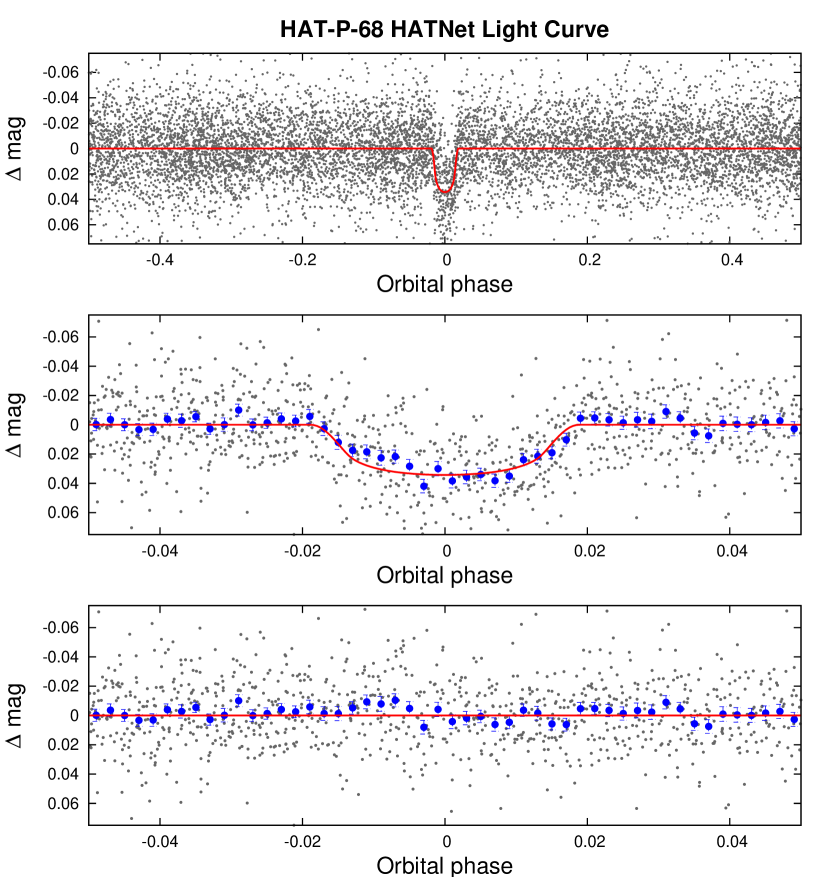
Figure 1: Discovery HATNet transit light curve phase-folded with a period of $2.2984$ days. Top: The full unbinned instrumental $r$ band light curve. The gray points show the individual measurements, while the solid red line shows the best-fit transit model. Middle: Same as the top panel, here we restrict the horizontal range of the plot to better display the transit. The filled blue circles show the light curve averaged in phase using a bin-size of 0.002. Bottom: The residuals from the best-fit transit model.

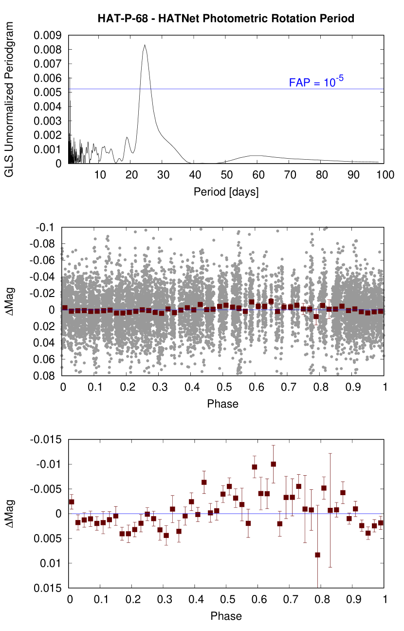
Figure 2: Detection of a $P=24.593\pm 0.064$ days photometric rotation period signal in the HATNet light curve of HAT-P-68. Top: The Generalized Lomb-Scargle (GLS) periodogram of the HATNet light curve after subtracting the best-fit transit model. The horizontal blue line shows a bootstrap-calibrated $10^{-5}$ false alarm probability (FAP) level. Middle: The HATNet light curve phase-folded at the peak GLS period. The gray points show the individual photometric measurements, while the dark red filled squares show the observations binned in phase with a bin size of 0.02. Bottom: Same as the middle panel, here we restrict the vertical range of the plot to better show the variation seen in the phase-binned measurements. We only show the phase binned measurements in this case as the variation in the un-binned points exceeds the vertical axis range of the plot.

Observations of a field containing HAT-P-68 were carried out between 2011 November and 2012 May by the HAT-5 and HAT-8 instruments located at FLWO and MKO, respectively. A total of 5867 and 3034 exposures of 3 minutes were obtained with each device through a Sloan $r$ filter, after which the images were reduced to trend-filtered light curves following Bakos et al. (2010). Here we used the Trend-Filtering Algorithm (TFA; Kovács et al., 2005) in signal-detection mode (i.e., the filtering was done before identifying the transit signal, and no attempt was made to preserve the shape of the transit during the filtering process). The final point-to-point precision for the HATNet light curve of HAT-P-68 is 2.4%.

We searched the light curves from the aforementioned field for periodic box-shaped transit events using the Box Least Squares method (BLS; Kovács et al., 2002), and detected 3.6% deep transits with a period of $2.2984$ days in the light curve of HAT-P-68. This detection prompted additional photometric and spectroscopic follow-up observations, as described in the subsections below. Figure 1 shows the HATNet light curve phase folded at the period identified with BLS, together with our best-fit transit model. The differential photometry data are made available in Table 2.4.

After subtracting the best-fit primary transit model from the HATNet light curve, we used BLS to search the residuals for additional periodic transit signals. No other significant transit signals were identified. We can place an approximate upper limit of 1% on the depth of any other periodic transit signals in the light curve with periods shorter than $\sim 10$ days.

To supplement the search for periodic transit signals, we also searched the HATNet light curve residuals for sinusoidal periodic variations using the Generalized Lomb-Scargle (GLS) periodogram (Zechmeister & Kürster, 2009). This search detected a $P=24.593\pm 0.064$ day periodic quasi-sinusoidal signal, from which we computed a bootstrap-calibrated false alarm probability of $10^{-10.3}$ and a periodogram signal-to-noise ratio of $36$ as described in Hartman & Bakos (2016). The GLS periodogram and phase-folded light curve are shown in Figure 2. We provisionally identify this as the photometric rotation period of the star, and note that the period and amplitude are in line with other mid K dwarf main sequence stars (e.g., Hartman et al., 2011).

2.2 Reconnaissance Spectroscopy

Initial reconnaissance spectroscopy observations of HAT-P-68 were obtained using the Astrophysical Research Consortium Echelle Spectrometer (ARCES; Wang et al., 2003) on the ARC 3.5 m telescope located at Apache Point Observatory (APO) in New Mexico. Using this facility, we obtained three $\Delta\lambda$/$\lambda\equiv R=18,000$ resolution spectra of HAT-P-68 on UT 2012 Oct 30, 2012 Nov 7, and 2013 Mar 3. These had exposure times of 3600 s, 2740 s, and 2740 s, respectively, yielding signal-to-noise ratios per resolution element near 5180 Å of 32.3, 25.6, and 26.8, respectively. The échelle images were reduced to wavelength-calibrated spectra following Hartman et al. (2015).

We applied the Stellar Parameter Classification (SPC; Buchhave et al., 2012) method on the échelle images to measure the RV and atmospheric parameters for the stellar host. In particular, this pipeline derives the effective temperature ($T_{\rm eff\star}$), surface gravity ($\log{g}$), metallicity ($\rm[Fe/H]$) and projected equatorial rotation velocity ($v\sin{i}$). Based on the three ARCES observations we estimated $T_{\rm eff\star}=4500\pm 50$ K, $\log{g}=4.62\pm 0.10$ (cgs), $\rm[Fe/H]=-0.14\pm 0.08$ and $v\sin{i}=2.5\pm 0.5$ $\rm km\,s^{-1}$.

We caution that the uncertainties based on this analysis are likely underestimated compared to the values reported in Section 3.1 based on an SPC analysis of Keck-I/HIRES observations. The three RV measurements were consistent with no variation, with a mean value of $-8.69$ $\rm km\,s^{-1}$, and a standard deviation of $0.43$ $\rm km\,s^{-1}$, comparable to the systematic uncertainties in the wavelength calibration. We note that the cross-correlation functions were consistent with a single K dwarf star, with no evidence of a second set of absorption lines present in the spectra.

2.3 High RV-Precision Spectroscopy

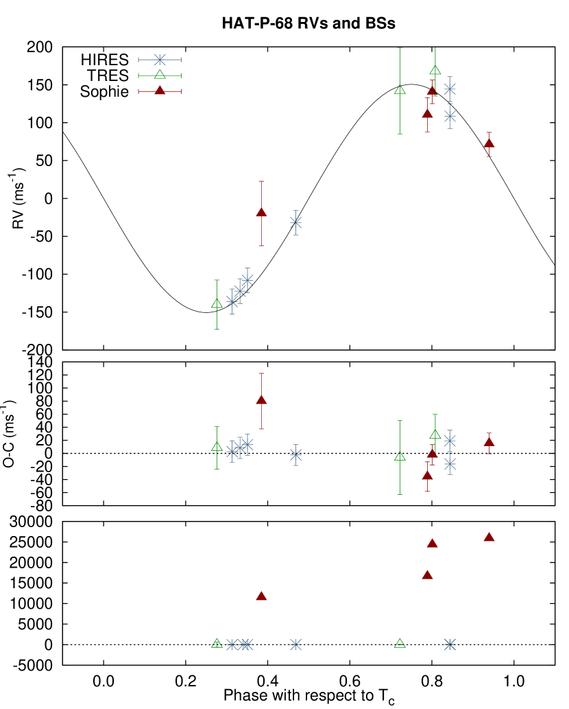
Figure 3: Top: High-precision RV measurements from FLWO 1.5 m/TRES, OHP 1.9 m/Sophie, and Keck-I 10 m/HIRES, together with our best-fit orbit model, plotted as a function of orbital phase. Phase zero corresponds to the time of mid transit. The center-of-mass velocity has been subtracted. The error bars include the jitter which is varied independently for each instrument in the fit. Middle: RV $O\!-\!C$ residuals from the best-fit model, plotted as a function of phase. Bottom: Spectral line bisector spans (BSs) plotted as a function of phase. Note the different vertical scales of the three panels.

Following the reconnaissance, we obtained higher resolution, and higher RV-precision spectroscopic observations of HAT-P-68 to further characterize it. To carry out these observations we used the Tillinghast Reflector Echelle Spectrograph (TRES; Fűresz, 2008) on the 1.5 m Tillinghast Reflector at FLWO, the Sophie spectrograph (Bouchy et al., 2009) on the Observatoire de Haute-Provence (OHP) 1.93 m in France, and HIRES (Vogt et al., 1994) on the Keck-I 10 m at MKO together with its I₂ absorption cell. The measured RVs and spectral line bisector spans (BSs) from these three facilities are provided in Table 2.3 and plotted in Figure 3.

A total of 3 TRES spectra were obtained on UT 2012 Nov 23, 2013 Mar 1, and 2013 Oct 11 at a resolution of $R=44,000$ and were reduced to high precision RVs and BSs following Bieryla et al. (2014), and to atmospheric stellar parameters using SPC.

A total of four $R=39,000$ spectra were obtained with Sophie on UT 2013 Oct 31, 2013 Nov 1, and 2013 Nov 6, and were reduced to high-precision RVs and BSs following Boisse et al. (2013).

A total of six $R=55,000$ spectra were obtained through an I₂ cell with HIRES on UT 2013 Oct 19, 2013 Dec 11–12, and 2015 Nov 26–28. An I₂-free template observation was obtained on UT 2013 Oct 19. These data were collected and reduced following standard procedures of the California Planet Search (CPS; Howard et al., 2010), including computation of RVs using a method descended from Butler et al. (1996), and BSs following Torres et al. (2007). We also applied SPC to the I₂-free template to obtain high precision atmospheric parameters of the host star. Note that while we did not have an RV observation for this observation, we did compute a BS measurement from the blue orders of the echelle for it.

As seen in Figure 3, the RVs from TRES, Sophie and HIRES exhibited a clear Keplerian orbital variation in phase with the ephemeris from the photometric transits. We also find that the BSs from HIRES show almost no variation. The TRES BS values had several hundred $\rm m\,s^{-1}$ uncertainties, and the Sophie values varied by many $\rm km\,s^{-1}$, in both cases due to significant sky contamination that affected the shapes of the cross correlation functions (CCFs).

Table 1: Summary of Spectroscopic Observations

Telescope/Instrument	UT Date(s)	# Spectra	Resolution	S/N Range	$\gamma_{RV}$	RV Precision
			$\Delta\lambda$/$\lambda$		($\rm m\,s^{-1}$)	($\rm m\,s^{-1}$)
APO 3.5 m/ARCES	2012 Oct–2013 Mar	3	18000	26.8–32.3	$-8600$	430
FLWO 1.5 m/TRES	2012 Nov–2013 Nov	3	44000	10–17	$-7960$	$16.8$
OHP 1.9 m/Sophie	2013 Oct–Nov	4	39000	26–43	$-8890$	$48.6$
Keck-I 10 m/HIRES	2013 Oct–2015 Nov	6	55000	81–115	$\cdots$	$12.5$

Table 2: Relative Radial Velocities and Bisector Spans of HAT-P-68.

BJD	RV	$\sigma_{\rm RV}$	BS	$\sigma_{\rm BS}$	Phase	Instrument
(2 450 000$+$)	($\rm m\,s^{-1}$)	($\rm m\,s^{-1}$)	($\rm m\,s^{-1}$)
$6255.01387$	$129.47$	$56.77$	$\cdots$	$\cdots$	$0.722$	TRES
$6352.82025$	$-152.51$	$32.59$	$\cdots$	$\cdots$	$0.276$	TRES
$6576.98851$	$155.31$	$32.59$	$\cdots$	$\cdots$	$0.808$	TRES
$6585.08850$	$-129.45$	$3.11$	$\cdots$	$\cdots$	$0.332$	HIRES
$6585.10625$	$\cdots$	$\cdots$	$-7.8$	$20.9$	$0.340$	HIRES
$6596.70034$	$-18.23$	$42.50$	$11517.0$	$85.0$	$0.384$	Sophie
$6597.63007$	$112.07$	$22.60$	$16666.0$	$45.2$	$0.789$	Sophie
$6597.65777$	$142.37$	$15.60$	$24376.0$	$31.2$	$0.801$	Sophie
$6602.57256$	$72.97$	$15.90$	$25886.0$	$31.8$	$0.939$	Sophie
$6637.99344$	$-115.18$	$2.68$	$4.9$	$34.7$	$0.350$	HIRES
$6639.12704$	$137.20$	$3.30$	$3.1$	$25.8$	$0.844$	HIRES
$7353.06851$	$-39.00$	$2.42$	$3.2$	$20.3$	$0.468$	HIRES
$7353.93251$	$101.52$	$3.14$	$51.3$	$63.6$	$0.844$	HIRES
$7355.01022$	$-143.22$	$4.11$	$-19.7$	$41.6$	$0.313$	HIRES

2.4 Photometric Follow-up

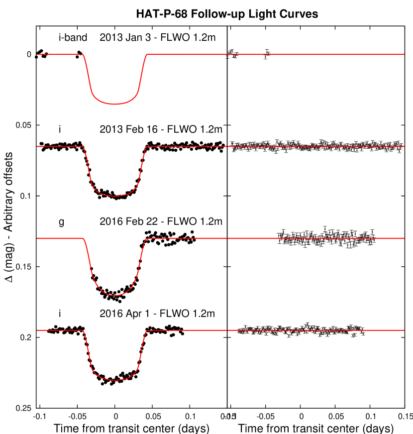
Figure 4: Unbinned follow-up transit light curves obtained with KeplerCam on the FLWO 1.2 m, plotted with the best-fit transit model as a solid red line. The dates of observation and photometric filters used are indicated. The residuals are shown on the right-hand side in the same order as the light curves.

In order to confirm the transit signal identified in the HATNet light curve of HAT-P-68, we carried out photometric follow-up observations of the system using the KeplerCam mosaic CCD imager on the FLWO 1.2 m telescope. Observations used in the analysis were conducted on five nights covering four predicted primary transit events, and one predicted secondary eclipse event. The nights, filters, number of exposures, effective cadences, and point-to-point photometric precision achieved are listed in Table 3. A sixth observation obtained on the night of 2013 Feb 10 did not observe either the primary transit or secondary eclipse, and was excluded from the analysis.

The KeplerCam CCD images were calibrated and reduced to light curves using the aperture photometry routine described by Bakos et al. (2010). We applied an External Parameter Decorrelation (EPD) and TFA-filtering of the light curves as part of the global modeling of the system, which we discuss further in Section 3. The four light curves covering the primary transit are shown in Figure 4. The light curve covering the predicted secondary eclipse was consistent with no eclipse variation, and was used in the blend analysis of the system, but was not included in the global analysis to determine the planetary and stellar parameters. All of the light curve data are made available in Table 2.4.

Table 3: Summary of Photometric Observations

Instrument/Field	Date(s)	# Images	Cadence	Filter	Precision
			(sec)		(mmag)
HAT-5/G268	2011 Nov–2012 May	5867	216	$r$	25.6
HAT-8/G268	2012 Jan–2012 Mar	3034	213	$r$	21.8
FLWO 1.2 m/KeplerCam	2013 Jan 03	18	194	$i$	3.5
FLWO 1.2 m/KeplerCam	2013 Feb 16	184	114	$i$	1.6
FLWO 1.2 m/KeplerCam	2016 Feb 22	102	118	$g$	3.3
FLWO 1.2 m/KeplerCam	2016 Mar 24	120	117	$i$	1.3
FLWO 1.2 m/KeplerCam	2016 Apr 01	133	118	$i$	1.8

Table 4: Differential Photometry of HAT-P-68

Note. — This table is available in a machine-readable form in the online journal. An abridged version is shown here for guidance regarding its form and content. The data are also available on the HATNet website at http://www.hatnet.org.

2.5 Search for Resolved Stellar Companions

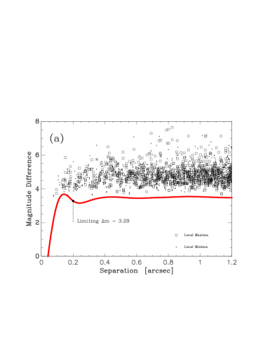
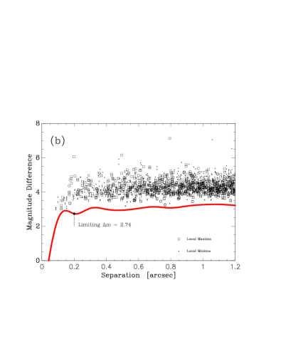
Figure 5: DSSI detection limits on the relative magnitude of a resolved companion for HAT-P-68 in the 692 nm (a) and 880 nm (b) filters. The plot shows the local maxima and minima data (in squares and points, respectively) as a function of angular separation. The solid red curves are cubic-spline interpolations of the 5$\sigma$ detection limit.

If there are nearby stellar companions to HAT-P-68, they would dilute the transit signal. In order to check for such companions we obtained high spatial resolution speckle imaging observations of HAT-P-68 with the Differential Speckle Survey Instrument (DSSI; Horch et al., 2009) on the WIYN 3.5 m telescope at Kitt Peak National Observatory in Arizona. The observations were gathered on the night of UT 27 October 2015. A dichroic beamsplitter was used to obtain simultaneous imaging through 692 nm and 880 nm filters.

Each observation consists of a sequence of 1000 40 ms exposures read-out on $128\times 128$ pixel ($2\farcs 8\times 2\farcs 8$) subframes, that are reduced to reconstructed images following Howell et al. (2011). These images were then searched for companions. Finding no companions to HAT-P-68 within $1\farcs 2$ when the ten observations of this system were combined, we place $5\sigma$ lower limits on the differential magnitude between a putative companion and the primary star as a function of angular separation following the method described in Horch et al. (2011).

Figure 5 shows the limiting-magnitude plots constructed from the reconstructed images, where the data represent local maxima and minima and the solid curve is a cubic-spline interpolation of the 5$\sigma$ detection limit. We find limiting magnitude differences at $0\farcs 2$ of $\Delta m_{692}=3.29$ and $\Delta m_{880}=2.74$.

In addition to the companion limits based on the WIYN 3.5 m/DSSI observations we also queried the UCAC 4 catalog (Zacharias et al., 2013), and the Gaia DR1 catalog (Gaia Collaboration et al., 2016) for neighbors within 20″ that may dilute either the HATNet or KeplerCam photometry. We find no such neighbors. Additionally, the Gaia DR2 catalog (Gaia Collaboration et al., 2018) shows no neighbors within 10″ of HAT-P-68.

3 Analysis

We analyzed the photometric and spectroscopic observations of HAT-P-68 to determine the parameters of the system using the most up-to-date procedures developed for HATNet and HATSouth (Hartman et al., 2019; Bakos et al., 2018). In the following, we briefly summarize our analysis methods to accurately determine the stellar and planetary physical parameters and to rule out various false positive scenarios.

3.1 Stellar Host Properties

High-precision stellar atmospheric parameters were measured from the I₂-free HIRES template spectrum using SPC, yielding $T_{\rm eff\star}=4514\pm 50$ K, $\rm[Fe/H]$$=-0.140\pm 0.080$, $v\sin{i}=0.0\pm 2.0$ $\rm km\,s^{-1}$, and $\log g_{\star}=4.67\pm 0.10$ (cgs). The resulting $T_{\rm eff\star}$ and $\rm[Fe/H]$ measurements were included in the global modeling to determine the physical stellar parameters.

We ultimately tried three methods to ascertain these physical parameters. The first two methods compare the observable properties to two different stellar evolution models. The last method uses empirical relations to derive stellar mass and radius.

3.1.1 Isochrone-based Parameters

Initially, we attempted to compare the Yonsei-Yale (Y²; Yi et al., 2001) models to the observed light-curve-based stellar density, and the spectroscopically determined values of $T_{\rm eff\star}$ and $\rm[Fe/H]$. This is the method that was followed, for example, in Bakos et al. (2010), and has been previously applied to the majority of published transiting planet discoveries from the HATNet project. Note that this was completed prior to the availability of Gaia DR2. Assuming a circular orbit, the best-fit stellar density is more than $3\sigma$ lower than the minimum density from theoretical models – that was achieved within the age of the Galaxy for a K dwarf star with a photosphere temperature of $4500$ K. This discrepancy between the measured stellar density and older stellar evolution models, such as the Y² models, has been previously reported for other mid K through early M dwarf stars (eg. Boyajian et al., 2012).

Fortunately, Chen et al. (2014b) improved the PAdova-TRieste Stellar Evolution Code (PARSEC; Bressan et al., 2012) models for very low mass stars ($<0.6M_{\sun}$) over a wide range of wavelengths. Randich et al. (2018) also demonstrated that Gaia parallaxes can be combined with ground-based datasets to yield robust stellar ages. As such, we opted to use PARSEC models combined with the Gaia DR2 data, following Hartman et al. (2019).

We performed a tri-linear interpolation within a grid of PARSEC model isochrones using $T_{\rm eff\star}$, $\rm[Fe/H]$, and the bulk stellar density $\rho_{\star}$ as the independent variables. These three variables in turn are directly varied in the global MCMC analysis (Section 3.2), or determined directly from parameters that are varied in this fit. The tri-linear interpolation then yields the $M_{\star}$, $R_{\star}$  $L_{\star}$, and age values to associate with each trial set of $T_{\rm eff\star}$, $\rm[Fe/H]$ and $\rho_{\star}$. Through this process we restrict the fit to consider only combinations of $T_{\rm eff\star}$, $\rm[Fe/H]$ and $\rho_{\star}$ that match to a stellar model. For K dwarf stars, such as HAT-P-68, which exhibit little evolution over the age of the Galaxy, this is a rather restrictive constraint. Including this constraint yields a posteriori estimates for the stellar atmospheric parameters of: $T_{\rm eff\star}=4508\pm 43$ K, $\rm[Fe/H]$$=-0.059\pm 0.036$, and $\log g_{\star}=4.615\pm 0.013$. Assuming a circular orbit, the PARSEC isochrone-based method yields a stellar mass and radius of $0.6785_{-0.0079}^{+0.0299}$ $M_{\sun}$ and $0.6701_{-0.0032}^{+0.0041}$ $R_{\sun}$, respectively, an age of $11.1_{-6.9}^{+1.1}$ Gyr, and a reddening-corrected distance of $202.93\pm 0.97$ pc.

3.1.2 Empirically Based Parameters

As an alternative approach, we also determined the stellar physical parameters following an empirical method similar to that of Stassun et al. (2017). This method effectively combines the bulk stellar density – measured from the transit light curve – with the stellar radius –measured from the effective temperature, parallax and apparent magnitudes in several band-passes – to determine the stellar mass. In practice this is incorporated into the global MCMC modeling (Section 3.2), and theoretical bolometric corrections are used to predict the absolute magnitude in each band-pass from the effective temperature, radius and metallicity of the star. Assuming a circular orbit, this empirical method yields a stellar mass and radius of $0.614\pm 0.055$ $M_{\sun}$ and $0.6720\pm 0.0075$ $R_{\sun}$, respectively, and a reddening-corrected distance of $203.46\pm 1.00$ pc. Note that these parameters are not restricted by the isochrones from PARSEC, which is why the uncertainties are larger compared to the uncertainties on the isochrone-based parameters.

3.2 Global Modeling

We determined the parameters of the system by carrying out a joint modeling of the high-precision RVs (fit using a Keplerian orbit), the HATNet and follow-up light curves (fit using a Mandel & Agol, 2002 transit model with Gaussian priors for the quadratic limb darkening coefficients taken from Claret et al., 2012, 2013 and Claret, 2018 to place Gaussian prior constraints on their values, assuming a prior uncertainty of $0.2$ for each coefficient), the catalog broad-band magnitudes, the stellar parallax from Gaia DR2, and the spectroscopically determined atmospheric parameters of the system. These latter stellar observations were modeled using isochrone and empirical-based methods, as discussed above (Section 3.1). This analysis makes use of a differential evolution Markov Chain Monte Carlo procedure (MCMC; ter Braak, 2006) to estimate the posterior parameter distributions, which we use to determine the median parameter values and their 1$\sigma$ uncertainties.

For each of the methods that we adopted to model the stellar parameters, we carried out two fits, one where the orbit is assumed to be circular, and another where the eccentricity parameters are allowed to vary in the fit. In both cases we allow the RV jitter (an extra term added in quadrature to the formal RV uncertainties) to vary independently for each of the instruments used. We find that when the isochrone-based stellar parameters are used, the free eccentricity model yields an eccentricity consistent with zero ($e=0.013\pm 0.013{}$), resulting in a 95% confidence upper limit on the eccentricity of $e<0.041{}$. We therefore adopt the following parameters for HAT-P-68b assuming a circular orbit: a mass of $0.724\pm 0.043$ $M_{\rm J}$, a radius of $1.072\pm 0.012$ $R_{\rm J}$, and an equilibrium temperature of $1027.8\pm 8.2{}$ K. The equilibrium temperature was calculated assuming zero albedo and full redistribution of heat. We give the planetary parameters derived from the joint fit, in Table 6. For comparison, when the empirical method is used, and a circular orbit is assumed, we find a planet mass of $0.711\pm 0.038$ $M_{\rm J}$, planet radius of $1.072\pm 0.015$ $R_{\rm J}$, and an equilibrium temperature of $1015.0_{-5.7}^{+14.9}{}$ K.

3.3 Adopted Parameters

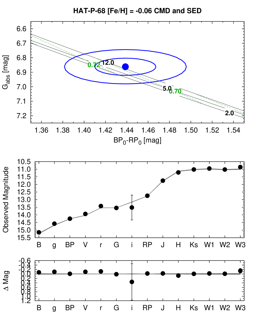
Figure 6: Top: The absolute Gaia G-band magnitude vs. the dereddened $BP-RP$ color. This measured value is compared to theoretical isochrones (black lines at Gyr ages in black) and stellar evolution tracks (green lines at solar masses in green) from the PARSEC models interpolated at the spectroscopically determined metallicity of the host. The filled blue circle show the measured reddening- and distance-corrected values from Gaia DR2, while the blue lines indicate the $1\sigma$ and $2\sigma$ confidence regions, including the estimated systematic errors in the photometry. Middle: The SED as measured via broadband photometry through the fourteen listed filters. We plot the observed magnitudes without correcting for distance or extinction. Over-plotted are 200 model SEDs randomly selected from the MCMC posterior distribution produced through the global analysis. Bottom: The residuals from the best-fit model SED.

We included in the global modeling analysis broad-band photometry from Gaia DR2, APASS (Henden et al., 2009), 2MASS (Skrutskie et al., 2006), and WISE (Wright et al., 2010) – $G$, $BP$, $RP$, $B$, $V$, $g$, $r$, $i$, $J$, $H$, $K_{s}$, $W1$, $W2$, and $W3$ bands. To account for dust extinction we included $A_{V}$ as a free-parameter in the model, assumed the Cardelli et al. (1989) $R_{V}=3.1$ extinction law, and placed a Gaussian prior on $A_{V}$ based on the predicted extinction from the MWDUST 3D Galactic extinction model (Bovy et al., 2016).

Figure 6 shows the comparison between the broadband photometric measurements and the PARSEC models mentioned in Section 3.1.1. The top panel is a color-magnitude diagram (CMD) of the Gaia $G$ magnitude versus the dereddened $BP-RP$ color as a filled blue circle, along with the $1\sigma$ and $2\sigma$ confidence regions in blue lines. We plot a set of $\rm[Fe/H]$=$0.06$ isochrones and stellar evolution tracks using black lines and green lines, respectively. The age of each isochrone is listed in black using Gyr units, while the mass of each evolution track is listed in green using solar mass units. The middle panel compares 200 model spectral energy distributions (SEDs) to the observed broadband photometry, the latter of which has not been corrected for distance or extinction. The bottom panel shows the residuals from the best-fit model SED. We find that the observed photometry and parallax is consistent with the models.

Based on the global MCMC analysis, we adopt parameters assuming a circular orbit for the isochrone-based method. We list the joint fit derived parameters in Tables 5 and  6.

3.4 Excluding False Positive Scenarios

In order to rule out the possibility that HAT-P-68 is a blended stellar eclipsing binary (EB) system, we carried out a direct blend analysis of the data following Hartman et al. (2012), with modifications from Hartman et al. (2019). We find that all blended stellar EB models tested can be ruled out – based on their fit to the photometry, parallax, and light curves – with almost $4\sigma$ confidence, and conclude that HAT-P-68 is a transiting planet system, and not a blended stellar EB system.

Note that the blend analysis of HAT-P-68 as an unresolved stellar binary with a planet around one stellar component provides a slight improvement to the fit compared to assuming no such unresolved stellar companion ($\Delta\chi^{2}$ value of $-2.93$), but the difference is consistent with the expected improvement from adding an additional parameter to the fit. Based on the high-spatial-resolution imaging that we have carried out (Section 2.5), any unresolved companion separated by more than $\sim 0\farcs 2$, must have $\Delta m>3.07$ at 692 nm compared to the transiting planet host. We conclude our findings assuming that there is no stellar companion.

Table 5: Stellar Parameters for HAT-P-68

Parameter	Value	Source
Identifiers
GSC-ID	1925-01046
2MASS-ID	07535598+2356176
Gaia DR2-ID	675443053940533760
Astrometric Properties
R.A. (h:m:s)	$07^{\mathrm{h}}53^{\mathrm{m}}55.9828{\mathrm{s}}$	Gaia DR2
Dec. (d:m:s)	$23{\arcdeg}56{\arcmin}17.6117{\arcsec}$	Gaia DR2
R.A.p.m. (mas/yr)	$-23.655\pm 0.039$	Gaia DR2
Dec.p.m. (mas/yr)	$-1.467\pm 0.022$	Gaia DR2
Parallax (mas)	$4.918\pm 0.023$	Gaia DR2
Spectroscopic Properties
$T_{\rm eff\star}$ (K)	$4514\pm 50$	SPC
$\rm[Fe/H]$	$-0.140\pm 0.080$	SPC
$v\sin{i}_{\star}$ ($\rm km\,s^{-1}$)	$0.0\pm 2.0$	SPC
Photometric Properties
$G$ (mag)	$13.54420\pm 0.00070$	Gaia DR2
$BP$ (mag)	$14.2484\pm 0.0028$	Gaia DR2
$RP$ (mag)	$12.7429\pm 0.0017$	Gaia DR2
$B$ (mag)	$15.148\pm 0.030$	APASS
$V$ (mag)	$13.937\pm 0.030$	APASS
$g$ (mag)	$14.578\pm 0.020$	APASS
$r$ (mag)	$13.421\pm 0.050$	APASS
$i$ (mag)	$13.52\pm 0.82$	APASS
$J$ (mag)	$11.750\pm 0.022$	2MASS
$H$ (mag)	$11.210\pm 0.023$	2MASS
$K_{s}$ (mag)	$11.019\pm 0.018$	2MASS
$W1$ (mag)	$10.956\pm 0.025$	WISE
$W2$ (mag)	$11.021\pm 0.021$	WISE
$W3$ (mag)	$10.86\pm 0.10$	WISE
$P_{\rm rot}$ (days)	$24.593\pm 0.064$	HATNet
Derived Properties
$M_{\star}$ ($M_{\sun}$)	$0.6785_{-0.0079}^{+0.0299}$	Global Modeling
$R_{\star}$ ($R_{\sun}$)	$0.6701_{-0.0032}^{+0.0041}$	Global Modeling
$\log{g_{\star}}$ (cgs)	$4.615\pm 0.013$	Global Modeling
$\rho_{\star}$ ($\rm g\,cm^{-3}$)	$3.165_{-0.046}^{+0.187}$	Global Modeling
$L_{\star}$ ($L_{\sun}$)	$0.1663\pm 0.0062$	Global Modeling
$T_{\rm eff\star}$ (K)	$4508\pm 43$	Global Modeling
$\rm[Fe/H]$	$-0.059\pm 0.036$	Global Modeling
Age (Gyr)	$11.1_{-6.9}^{+1.1}$	Global Modeling
$A_{V}$ (mag)	$0.180\pm 0.075$	Global Modeling
Distance (pc)	$202.93\pm 0.97$	Global Modeling

Table 6: Parameters for the planet HAT-P-68b.

Parameter	Value	Parameter	Value
Light curve parameters		RV parameters
$P$ (days)	$2.29840551\pm 0.00000052{}$	$K$ ($\rm m\,s^{-1}$)	$143.4\pm 8.4{}$
$T_{c}$ (${\rm BJD}$)	$2456614.20355\pm 0.00014{}$	$e$	$<0.041{}$
$T_{14}$ (days)	$0.08695\pm 0.00053{}$	HIRES RV jitter ($\rm m\,s^{-1}$)	$14.3\pm 7.9$
$T_{12}=T_{34}$ (days)	$0.01279\pm 0.00033{}$	TRES RV jitter ($\rm m\,s^{-1}$)	$0\pm 25$
$a/R_{\star}$	$9.600_{-0.047}^{+0.185}{}$	Sophie RV jitter ($\rm m\,s^{-1}$)	$0\pm 59$
$\zeta/R_{\star}$	$26.95\pm 0.21{}$	Planetary parameters
$R_{p}/R_{\star}$	$0.1644\pm 0.0015{}$	$M_{p}$ ($M_{\rm J}$)	$0.724\pm 0.043{}$
$b^{2}$	$0.045_{-0.026}^{+0.021}{}$	$R_{p}$ ($R_{\rm J}$)	$1.072\pm 0.012{}$
$b\equiv a\cos i/R_{\star}$	$0.212_{-0.076}^{+0.045}{}$	$C(M_{p},R_{p})$	$-0.04{}$
$i$ (deg)	$88.73_{-0.27}^{+0.47}{}$	$\rho_{p}$ ($\rm g\,cm^{-3}$)	$0.727\pm 0.051{}$
Limb-darkening coefficients		$\log g_{p}$ (cgs)	$3.192\pm 0.029{}$
$c_{1},g$ (linear term)	$0.718\pm 0.097{}$	$a$ (AU)	$0.02996_{-0.00012}^{+0.00043}{}$
$c_{2},g$ (quadratic term)	$0.25\pm 0.11{}$	$T_{\rm eq}$ (K)	$1027.8\pm 8.2{}$
$c_{1},r$	$0.49\pm 0.14{}$	$\Theta$	$0.0590\pm 0.0035{}$
$c_{2},r$	$0.41\pm 0.15{}$	$\langle F\rangle$ ($\rm erg\,s^{-1}\,cm^{-2}$)	$(2.515\pm 0.080{})\times 10^{8}$
$c_{1},i$	$0.337\pm 0.073{}$
$c_{2},i$	$0.34\pm 0.14{}$

4 Discussion

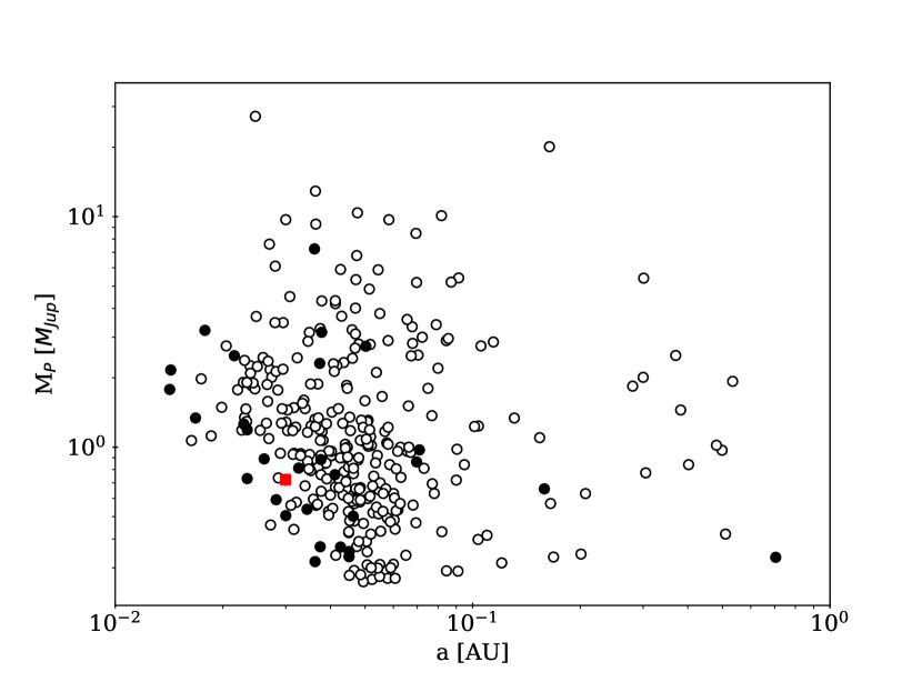
Figure 7: Planet mass as a function of semi-major axis for all known giant ($M_{P}>0.25M_{\rm J}$) planets with measured masses and radii. We differentiate host star masses by plotting the data for stars with $<0.8M_{\sun}$ (as filled black circles), for stars with $>0.8M_{\sun}$ (as unfilled black circles), and for HAT-P-68b (red square with errorbars). Data from NASA Exoplanet Archive as of 2020 September 24.

In this paper we have presented the discovery of the HAT-P-68 transiting planet system by the HATNet survey. We have found that every $2.2984{}$ days, the planet HAT-P-68b – with a mass of $0.724\pm 0.043$ $M_{\rm J}$, and radius of $1.072\pm 0.012$ $R_{\rm J}$, – orbits a star of mass $0.6785_{-0.0079}^{+0.0299}$ $M_{\sun}$, and radius $0.6701_{-0.0032}^{+0.0041}$ $R_{\sun}$. As such, the discovery of this planet contributes to the relatively small sample of low-mass (late K dwarf, and M dwarf) stars with known transiting giant planets.

We compared the newly discovered planet to the previously discovered planets listed in the NASA Exoplanet Archive as of 2020 September 24. With a semi-major axis of $a$=$0.02996_{-0.00012}^{+0.00043}{}$ AU, this planet joins the small but growing sample of 28 known giant planets in sub-0.05 AU orbits around low mass stars ($<0.8M_{\sun}$). Here, we restrict the sample of confirmed planets to those with well-measured masses greater than $0.25M_{\rm J}$, following Dawson & Johnson (2018). To demonstrate the significance of this planet, we show HAT-P-68b (red square with errorbars) in context with these HJs in Figure 7. The data for stars less massive than $0.8M_{\sun}$ are filled black circles, while data for stars more massive than $0.8M_{\sun}$ are unfilled black circles.

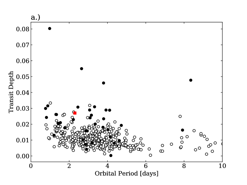
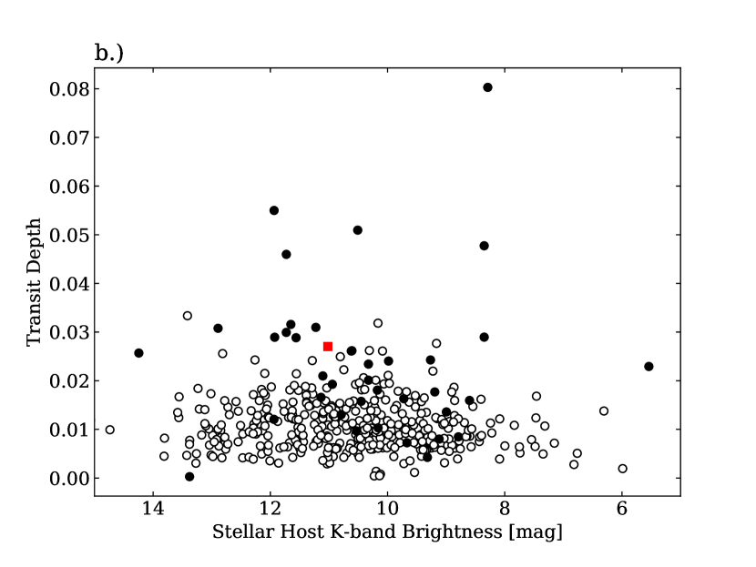
Figure 8: Transit depth as a function of (a.) orbital period for hot Jupiters and (b.) host K-band magnitude. The depth was calculated from the planetary radius $R_{P}$ and stellar radius $R_{\star}$. We differentiate host star masses by plotting the data for stars with $<0.8M_{\sun}$ (as filled black circles), for stars with $>0.8M_{\sun}$ (as unfilled black circles), and for HAT-P-68b (red square with errorbars). Data from NASA Exoplanet Archive as of 2020 September 24.

We find that including HAT-P-68b, there are 11 planetary systems with transit depths $>2.5\%$, which may be good targets for transmission spectroscopy. Of these other worlds, those that have already been studied using transmission spectroscopy include WASP-80b (Mancini et al., 2014; Kirk et al., 2017), WASP-52b (Kirk et al., 2016; Louden et al., 2017) and WASP-43b (Chen et al., 2014a; Weaver et al., 2020). While HAT-P-68 is much fainter than these hosts in the optical band-pass, it is only 1 mag fainter than WASP-52 in the $K$-band. In figure 8, we plot show the transit depths of HJs as a function of period (a.) and as a function of K-band stellar brightness magnitude (b.), where the depths were calculated from the planetary radius $R_{P}$ and stellar radius $R_{\star}$. Note that $(R_{P}/R_{\star})^{2}$ is an easy to compute proxy for the transit depth.

Finally, we note that HAT-P-68 is at an ecliptic latitude of $+3^{\circ}$, and is thus outside the field of view of the primary NASA TESS mission. It also was not observed during the K2 mission. The discovery of this planet by HATNet demonstrates that in the era of wide-field space-based transit surveys, interesting planets amenable to detailed characterization remain to be discovered, even from the ground.

Acknowledgements

HATNet operations have been funded by NASA grants NNG04GN74G as well as NNX13AJ15G. Follow-up of HATNet targets has been partially supported through NSF grant AST-1108686. B.L. is supported by the NSF Graduate Research Fellowship, grant no. DGE 1762114. J.H. acknowledges support from NASA grant NNX14AE87G. G.B., J.H. and W.B. acknowledge partial support from NASA grant NNX17AB61G. K.P. acknowledges support from NASA grant 80NSSC18K1009. I.B. thanks EuropeanCommunity’s Seventh Framework Programme (FP7/2007-2013) under grant agreement number RG226604 (OPTICON). and the Programme National dePlanétologie” (PNP) of CNRS/INSU We acknowledge partial support from the Kepler Mission under NASA Cooperative Agreement NCC2-1390 (D.W.L., PI). Data presented in this paper are based on observations obtained at the HAT station at the Submillimeter Array of SAO, and the HAT station at the Fred Lawrence Whipple Observatory of SAO. We acknowledge the use of the AAVSO Photometric All-Sky Survey (APASS), funded by the Robert Martin Ayers Sciences Fund, and the SIMBAD database, operated at CDS, Strasbourg, France. Data presented herein were obtained at the WIYN Observatory from telescope time allocated to NN-EXPLORE through the scientific partnership of the National Aeronautics and Space Administration, the National Science Foundation, and the National Optical Astronomy Observatory. This work was supported by a NASA WIYN PI Data Award, administered by the NASA Exoplanet Science Institute. This work has made use of data from the European Space Agency (ESA) mission Gaia, processed by the Gaia Data Processing and Analysis Consortium (DPAC, ). Funding for the DPAC has been provided by national institutions, in particular the institutions participating in the Gaia Multilateral Agreement. This research has made use of the NASA Exoplanet Archive, which is operated by the California Institute of Technology, under contract with the National Aeronautics and Space Administration under the Exoplanet Exploration Program. The authors wish to recognize and acknowledge the very significant cultural role and reverence that the summit of Mauna Kea has always had within the indigenous Hawaiian community. We are most fortunate to have the opportunity to conduct observations from this mountain.

References

- Astropy Collaboration et al. (2013) Astropy Collaboration, Robitaille, T. P., Tollerud, E. J., et al. 2013, A&A, 558, A33
- Auvergne et al. (2009) Auvergne, M., Bodin, P., Boisnard, L., et al. 2009, A&A, 506, 411
- Bakos et al. (2004) Bakos, G., Noyes, R. W., Kovács, G., et al. 2004, PASP, 116, 266
- Bakos (2018) Bakos, G. Á. 2018, The HATNet and HATSouth Exoplanet Surveys, 111
- Bakos et al. (2010) Bakos, G. Á., Torres, G., Pál, A., et al. 2010, ApJ, 710, 1724
- Bakos et al. (2013) Bakos, G. Á., Csubry, Z., Penev, K., et al. 2013, PASP, 125, 154
- Bakos et al. (2018) Bakos, G. Á., Bayliss, D., Bento, J., et al. 2018, arXiv e-prints, arXiv:1812.09406
- Bieryla et al. (2014) Bieryla, A., Hartman, J. D., Bakos, G. Á., et al. 2014, AJ, 147, 84
- Boisse et al. (2013) Boisse, I., Hartman, J. D., Bakos, G. Á., et al. 2013, A&A, 558, A86
- Borucki et al. (2010) Borucki, W. J., Koch, D., Basri, G., et al. 2010, Science, 327, 977
- Bouchy et al. (2009) Bouchy, F., Hébrard, G., Udry, S., et al. 2009, A&A, 505, 853
- Bovy et al. (2016) Bovy, J., Rix, H.-W., Green, G. M., Schlafly, E. F., & Finkbeiner, D. P. 2016, ApJ, 818, 130
- Boyajian et al. (2012) Boyajian, T. S., von Braun, K., van Belle, G., et al. 2012, ApJ, 757, 112
- Bressan et al. (2012) Bressan, A., Marigo, P., Girardi, L., et al. 2012, MNRAS, 427, 127
- Buchhave et al. (2012) Buchhave, L. A., Latham, D. W., Johansen, A., et al. 2012, Nature, 486, 375
- Butler et al. (1996) Butler, R. P., Marcy, G. W., Williams, E., et al. 1996, PASP, 108, 500
- Cardelli et al. (1989) Cardelli, J. A., Clayton, G. C., & Mathis, J. S. 1989, ApJ, 345, 245
- Charbonneau et al. (2002) Charbonneau, D., Brown, T. M., Noyes, R. W., & Gilliland, R. L. 2002, ApJ, 568, 377
- Chen et al. (2014a) Chen, G., van Boekel, R., Wang, H., et al. 2014a, A&A, 563, A40
- Chen et al. (2014b) Chen, Y., Girardi, L., Bressan, A., et al. 2014b, MNRAS, 444, 2525
- Claret (2004) Claret, A. 2004, A&A, 428, 1001
- Claret (2018) —. 2018, A&A, 618, A20
- Claret et al. (2012) Claret, A., Hauschildt, P. H., & Witte, S. 2012, A&A, 546, A14
- Claret et al. (2013) —. 2013, A&A, 552, A16
- Dawson & Johnson (2018) Dawson, R. I., & Johnson, J. A. 2018, ARA&A, 56, 175
- Fűresz (2008) Fűresz, G. 2008, PhD thesis, Univ. of Szeged, Hungary
- Gaia Collaboration et al. (2016) Gaia Collaboration, Brown, A. G. A., Vallenari, A., et al. 2016, A&A, 595, A2
- Gaia Collaboration et al. (2018) —. 2018, A&A, 616, A1
- Gaudi et al. (2005) Gaudi, B. S., Seager, S., & Mallen-Ornelas, G. 2005, ApJ, 623, 472
- Hansen & Barman (2007) Hansen, B. M. S., & Barman, T. 2007, ApJ, 671, 861
- Hartman & Bakos (2016) Hartman, J. D., & Bakos, G. Á. 2016, Astronomy and Computing, 17, 1
- Hartman et al. (2011) Hartman, J. D., Bakos, G. Á., Noyes, R. W., et al. 2011, AJ, 141, 166
- Hartman et al. (2012) Hartman, J. D., Bakos, G. Á., Béky, B., et al. 2012, AJ, 144, 139
- Hartman et al. (2015) Hartman, J. D., Bhatti, W., Bakos, G. Á., et al. 2015, AJ, 150, 168
- Hartman et al. (2016) Hartman, J. D., Bakos, G. Á., Bhatti, W., et al. 2016, AJ, 152, 182
- Hartman et al. (2019) Hartman, J. D., Bakos, G. Á., Bayliss, D., et al. 2019, AJ, 157, 55
- Henden et al. (2009) Henden, A. A., Welch, D. L., Terrell, D., & Levine, S. E. 2009, in American Astronomical Society Meeting Abstracts, Vol. 214, American Astronomical Society Meeting Abstracts #214, #407.02
- Horch et al. (2011) Horch, E. P., van Altena, W. F., Howell, S. B., Sherry, W. H., & Ciardi, D. R. 2011, AJ, 141, 180
- Horch et al. (2009) Horch, E. P., Veillette, D. R., Baena Gallé, R., et al. 2009, AJ, 137, 5057
- Howard et al. (2010) Howard, A. W., Johnson, J. A., Marcy, G. W., et al. 2010, ApJ, 721, 1467
- Howell et al. (2011) Howell, S. B., Everett, M. E., Sherry, W., Horch, E., & Ciardi, D. R. 2011, AJ, 142, 19
- Howell et al. (2014) Howell, S. B., Sobeck, C., Haas, M., et al. 2014, PASP, 126, 398
- Kirk et al. (2016) Kirk, J., Wheatley, P. J., Louden, T., et al. 2016, MNRAS, 463, 2922
- Kirk et al. (2017) Kirk, J., Wheatley, P. J., Louden, T., et al. 2017, MNRAS, 474, 876
- Kovács et al. (2005) Kovács, G., Bakos, G., & Noyes, R. W. 2005, MNRAS, 356, 557
- Kovács et al. (2002) Kovács, G., Zucker, S., & Mazeh, T. 2002, A&A, 391, 369
- Louden et al. (2017) Louden, T., Wheatley, P. J., Irwin, P. G. J., Kirk, J., & Skillen, I. 2017, MNRAS, 470, 742
- Mancini et al. (2014) Mancini, L., Southworth, J., Ciceri, S., et al. 2014, A&A, 562, A126
- Mandel & Agol (2002) Mandel, K., & Agol, E. 2002, ApJ, 580, L171
- Mayor & Queloz (1995) Mayor, M., & Queloz, D. 1995, Nature, 378, 355
- Morton & Winn (2014) Morton, T. D., & Winn, J. N. 2014, ApJ, 796, 47
- Nielsen et al. (2020) Nielsen, L. D., Brahm, R., Bouchy, F., et al. 2020, A&A, 639, A76
- Pál (2012) Pál, A. 2012, MNRAS, 421, 1825
- Pollacco et al. (2006) Pollacco, D., Skillen, I., Cameron, A. C., et al. 2006, PASP, 118, 1407
- Price-Whelan et al. (2018) Price-Whelan, A. M., Sipőcz, B. M., Günther, H. M., et al. 2018, AJ, 156, 123
- Randich et al. (2018) Randich, S., Tognelli, E., Jackson, R., et al. 2018, A&A, 612, A99
- Ricker et al. (2014) Ricker, G. R., Winn, J. N., Vanderspek, R., et al. 2014, Journal of Astronomical Telescopes, Instruments, and Systems, 1, 1
- Sestovic et al. (2018) Sestovic, M., Demory, B.-O., & Queloz, D. 2018, A&A, 616, A76
- Skrutskie et al. (2006) Skrutskie, M. F., Cutri, R. M., Stiening, R., et al. 2006, AJ, 131, 1163
- Stassun et al. (2017) Stassun, K. G., Collins, K. A., & Gaudi, B. S. 2017, AJ, 153, 136
- ter Braak (2006) ter Braak, C. J. F. 2006, Statistics and Computing, 16, 239
- Torres et al. (2007) Torres, G., Bakos, G. Á., Kovács, G., et al. 2007, ApJ, 666, L121
- Vogt et al. (1994) Vogt, S. S., Allen, S. L., Bigelow, B. C., et al. 1994, in Society of Photo-Optical Instrumentation Engineers (SPIE) Conference Series, Vol. 2198, Society of Photo-Optical Instrumentation Engineers (SPIE) Conference Series, ed. D. L. Crawford & E. R. Craine, 362
- Wang et al. (2003) Wang, S.-i., Hildebrand, R. H., Hobbs, L. M., et al. 2003, in Society of Photo-Optical Instrumentation Engineers (SPIE) Conference Series, Vol. 4841, Instrument Design and Performance for Optical/Infrared Ground-based Telescopes, ed. M. Iye & A. F. M. Moorwood, 1145–1156
- Weaver et al. (2020) Weaver, I. C., López-Morales, M., Espinoza, N., et al. 2020, AJ, 159, 13
- Wright et al. (2010) Wright, E. L., Eisenhardt, P. R. M., Mainzer, A. K., et al. 2010, AJ, 140, 1868
- Yi et al. (2001) Yi, S., Demarque, P., Kim, Y.-C., et al. 2001, ApJS, 136, 417
- Zacharias et al. (2013) Zacharias, N., Finch, C. T., Girard, T. M., et al. 2013, AJ, 145, 44
- Zechmeister & Kürster (2009) Zechmeister, M., & Kürster, M. 2009, A&A, 496, 577