Spline-Based Adaptive Cancellation of Even-Order Intermodulation Distortions in LTE-A/5G RF Transceivers

Abstract

Radio frequency transceivers operating in in-band full-duplex or frequency-division duplex mode experience strong transmitter leakage. Combined with receiver nonlinearities, this causes intermodulation products in the baseband, possibly with higher power than the desired receive signal. In order to restore the receiver signal-to-noise ratio in such scenarios, we propose two novel digital self-interference cancellation approaches based on spline interpolation. Both employ a Wiener structure, thereby matching the baseband model of the intermodulation effect. Unlike most state-of-the-art spline-based adaptive learning schemes, the proposed concept allows for complex-valued in- and output signals. The optimization of the model parameters is based on the stochastic gradient descent concept, where the convergence is supported by an appropriate step-size normalization. Additionally, we provide a gain control scheme and enable pipelining in order to facilitate a hardware implementation. An optional input transform improves the performance consistency for correlated sequences. In a realistic interference scenario, the proposed algorithms clearly outperform a state-of-the-art least mean squares variant with comparable complexity, which is specifically tailored to second-order intermodulation distortions. The high flexibility of the spline interpolation allows the spline-based Wiener models to match the performance of the kernel recursive least squares algorithm at less than 0.6 % of the arithmetic operations.

I Introduction

Power efficiency is a key aspect for RF transceivers in mobile communications equipment in order to ensure sufficient battery life at high data rates. Combined with other metrics, such as cost or area usage, this might lead to a decrease in receiver linearity. Given the low powers of the wanted Rx signal at the input, these design trade-offs usually do not cause relevant distortions. However, in IBFD and FDD operation, a strong Tx leakage in the receiver is unavoidable, leading to a severe deterioration of the Rx signal. When using the predominant direct-conversion receiver architecture, especially even-order IMD are a major issue, since they fall directly into the Rx BB independent of the Tx carrier frequency [1].

LTE In the Long-Term Evolution Advanced (LTE-A) and 5G NR standards, an important transmission mode is FDD. The resulting separation of the Tx and Rx carriers enables the usage of band-selection filters, in communication transceivers these are typically duplexers. These components provide a limited suppression of the transmitter-to-receiver leakage of about $5055\text{\,}\mathrm{dB}\text{/}$ [2]. A higher isolation is not feasible due to disadvantages such as higher cost or increased insertion losses. With Tx powers of up to $27\text{\,}\mathrm{dBm}\text{/}$ at the output of the PA, the spectrally shaped leakage still has considerable power at the duplexer Rx port, causing IMD. Besides design changes in the AFE, several BB mitigation techniques exist to attenuate the IMD interference [3]. In this work, we focus on fully digital self-interference cancellation for FDD transceivers, where the interference is replicated based on the known Tx data. While increasing the computational burden in the digital BB compared to mixed-signal solutions, DSIM approaches do not require any changes to the AFE and scale well with smaller technology nodes. Most published approaches target second-order intermodulation products, both, with [4, 5, 6, 7] and without [8, 9] a frequency-selective leakage path. However, also higher-order products are likely to occur but are rarely covered in literature [10, 11]. One category of suitable algorithms are general learning schemes, such as KAF, SVM or ANN with constant or adaptive activation functions [12, 13, 14, 15, 16, 17]. Other concepts are adaptive truncated Volterra series and functional link adaptive filters [18, 12], which both utilize limited model knowledge. However, these models result in an unreasonably high number of parameters to be estimated, slowing down adaptation and increasing complexity. The generation of higher-order IMD is best represented by Wiener models, but the required nonlinear estimation is often assumed to be unsuitable for real-time implementation on devices with limited computational resources. With the development of SAF [19, 20, 21], low-complex adaptive Wiener models for a wide range of nonlinearities are available. However, most of them target real-valued functions and, thus, are not applicable to the complex-valued IMD cancellation problem. Two exceptions featuring spline interpolation with complex control points are presented in [22, 23]. Though, both show specialized concepts without normalization, which are not suited for the IMD problem.

In this work, we introduce two novel Wiener SAF, comprised of a complex-valued linear system, a fixed internal nonlinearity and a real- or complex-valued spline output. The latter is achieved by combining two real-valued spline functions, where one models the real and one the imaginary part of the output. Both proposed SAF variants allow for a filtered output, which, for example, can cover a delayed update as it is caused by a pipelined hardware implementation. For the first time, internal clipping is avoided by means of an optimization constraint, that controls the norm of the linear filter weights. Additionally, an alternative limiter for the weight norm with lower complexity is proposed. The SGD update used for learning is improved by means of an appropriate novel step-size normalization. Optionally, the learning is augmented with the well-known TD concept to improve the performance consistency of the algorithms.

This paper is organized as follows: In Section II, we provide an in-depth analysis of the IMD effect, leading to a BB model that is essential for all further considerations. For completeness, in Section III, we give a brief overview of the spline interpolation concept. In Section IV, we derive normalized SGD update equations for the proposed SAF, discuss possible optimizations and assess the computational complexity. Section V quantifies the IMD cancellation performance of our concepts on a real-world scenario.

II Self-Interference Due To Intermodulation Distortions

Figure 1: Block diagram of FDD RF transceiver with digital cancellation of IMDx interference.

Fig. 1 schematically depicts one Tx and one Rx path of FDD transceiver, operating simultaneously on a common antenna. As a consequence of non-ideal Tx-Rx isolation in the analog front-end, the Tx signal leaks into the receiver, where it causes nonlinear distortions that overlay the wanted Rx BB signal. Note that in case of carrier aggregation, this problem potentially persists for all combinations of Tx and Rx chains.

A partial modeling of this effect is shown in [6, 24], which we use as a foundation to derive the interference components that occur in the Rx BB. Compared to the available literature, we include all important cross-terms of Tx leakage, wanted Rx and noise. This thorough analysis is essential in order to correctly interpret measurement results on the IMD effect. We start with the known digital Tx BB sequence $x_{\text{BB}}[n]$, which first passes the DAC. Next, the analog signal $x_{\text{BB}}(t)$ is up-converted to the carrier $f_{\text{Tx}}$. Since we focus on receiver nonlinearities, for our model we assume the up-conversion mixer and the PA to be ideal with a total gain of $A_{\text{PA}}$. This simplification is backed by simulations in Section V, where we include the saturation behavior of the PA. The cancellation performance of the proposed Wiener SAF is not impacted by the PA nonlinearity. After up-conversion and amplification, the resulting Tx RF signal is

$$x_{\text{RF}}(t)=A_{\text{PA}}\,\Re\left\{x_{\text{BB}}(t)\,e^{j2\pi f_{\text{Tx}}t}\right\}.$$ (1)

The leakage path, comprising RF switches, diplexers and the duplexer, is modeled as

$$h_{\text{RF}}^{\text{TxL}}(t)=2\,\Re\left\{h_{\text{BB}}^{\text{TxL}}(t)\,e^{j2\pi f_{\text{Tx}}t}\right\}$$ (2)

with the equivalent BB impulse response $h_{\text{BB}}^{\text{TxL}}(t)$. Depending on the context, $*$ denotes the time-continuous or time-discrete convolution. The factor $2$ is introduced in the RF domain to compensate for the scaling effect of the convolution later on. With these definitions, the RF leakage signal can be written as:

$$y_{\text{RF}}^{\text{TxL}} =x_{\text{RF}}(t)*h_{\text{RF}}^{\text{TxL}}(t)$$

$$=\frac{A_{\text{PA}}}{2}\left(x_{\text{BB}}(t)\,e^{j2\pi f_{\text{Tx}}t}+x_{\text{BB}}(t)^{*}\,e^{-j2\pi f_{\text{Tx}}t}\right)$$

$$\hskip 70.0001pt*\left(h_{\text{BB}}^{\text{TxL}}(t)\,e^{j2\pi f_{\text{Tx}}t}+h_{\text{BB}}^{\text{TxL}}(t)^{*}\,e^{-j2\pi f_{\text{Tx}}t}\right)$$

$$=\frac{A_{\text{PA}}}{2}\left(x_{\text{BB}}(t)*h_{\text{BB}}^{\text{TxL}}(t)\right)e^{j2\pi f_{\text{Tx}}t}$$

$$\hskip 70.0001pt+\frac{A_{\text{PA}}}{2}\left(x_{\text{BB}}(t)*h_{\text{BB}}^{\text{TxL}}(t)\right)^{*}e^{-j2\pi f_{\text{Tx}}t}$$

$$=\Re\left\{y_{\text{BB}}^{\text{TxL}}(t)\,e^{j2\pi f_{\text{Tx}}t}\right\}.$$ (3)

${y_{\text{BB}}^{\text{TxL}}(t)=x_{\text{BB}}(t)*\tilde{h}_{\text{BB}}^{\text{TxL}}(t)}$ is the BB equivalent leakage signal. To shorten the notation, we include the Tx gain in the impulse response of the leakage path ${\tilde{h}_{\text{BB}}^{\text{TxL}}(t)=A_{\text{PA}}h_{\text{BB}}^{\text{TxL}}(t)}$. Due to the leakage, the total signal at the receiver input is

$$y_{\text{RF}}^{\text{Tot}}(t)=y_{\text{RF}}^{\text{Rx}}(t)+\eta_{\text{RF}}(t)+y_{\text{RF}}^{\text{TxL}}(t).$$ (4)

$y_{\text{RF}}^{\text{Rx}}(t)$ is the desired receive signal at the carrier $f_{\text{Rx}}$

$$y_{\text{RF}}^{\text{Rx}}(t)=\Re\left\{y_{\text{BB}}^{\text{Rx}}(t)\,e^{j2\pi f_{\text{Rx}}t}\right\}$$ (5)

and $\eta_{\text{RF}}(t)$ is additive thermal noise from the antenna. Both components passed the duplexer and are therefore limited to the bandwidth of the selected LTE/NR band. However, any noise components that are added after the duplexer might have substantially higher bandwidth. In order to limit the complexity of the model, we neglect any wideband noise in the following and define

$$\eta_{\text{RF}}(t)=\Re\left\{\eta_{\text{BB}}(t)\,e^{j2\pi f_{\text{Rx}}t}\right\}.$$ (6)

Any components up to the quadrature mixer (I/Q mixer) potentially exhibit nonlinear behavior, which is modeled to be concentrated in the LNA and the mixer.

Based on measurements of the IMD products generated by an integrated CMOS receiver we assume a polynomial nonlinearity of degree 3 for modeling the LNA [25, 26]:

$$y_{\text{RF}}^{\text{LNA}}(t)=\alpha_{1}\,y_{\text{RF}}^{\text{Tot}}(t)+\alpha_{2}\left(y_{\text{RF}}^{\text{Tot}}(t)\right)^{2}+\alpha_{3}\left(y_{\text{RF}}^{\text{Tot}}(t)\right)^{3}.$$ (7)

The coefficients $\alpha_{i}$ are real-valued quantities. Inserting $y_{\text{RF}}^{\text{Tot}}(t)$ into the LNA model yields

$$y_{\text{RF}}^{\text{LNA}}(t) =\alpha_{1}\left(y_{\text{RF}}^{\text{Rx}}(t)+\eta_{\text{RF}}(t)+y_{\text{RF}}^{\text{TxL}}(t)\right)$$

$$\phantom{{}={}}+\alpha_{2}\,\Big{(}\!\left(y_{\text{RF}}^{\text{Rx}}(t)\right)^{2}+\left(\eta_{\text{RF}}(t)\right)^{2}+\left(y_{\text{RF}}^{\text{TxL}}(t)\right)^{2}$$

$$\phantom{{}={}+\alpha_{2}\,\Big{(}}+2\,y_{\text{RF}}^{\text{Rx}}(t)\,\eta_{\text{RF}}(t)+2\,y_{\text{RF}}^{\text{Rx}}(t)\,y_{\text{RF}}^{\text{TxL}}(t)$$

$$\phantom{{}={}+\alpha_{2}\,\Big{(}}+2\,\eta_{\text{RF}}(t)\,y_{\text{RF}}^{\text{TxL}}(t)\Big{)}$$

$$\phantom{{}={}}+\alpha_{3}\,\Big{(}\!\left(y_{\text{RF}}^{\text{Rx}}(t)\right)^{3}+\left(\eta_{\text{RF}}(t)\right)^{3}+\left(y_{\text{RF}}^{\text{TxL}}(t)\right)^{3}$$

$$\phantom{{}={}+\alpha_{3}\,\Big{(}}+3\left(y_{\text{RF}}^{\text{Rx}}(t)\right)^{2}\eta_{\text{RF}}(t)+3\left(y_{\text{RF}}^{\text{Rx}}(t)\right)^{2}y_{\text{RF}}^{\text{TxL}}(t)$$

$$\phantom{{}={}+\alpha_{3}\,\Big{(}}+3\,y_{\text{RF}}^{\text{Rx}}(t)\,\left(\eta_{\text{RF}}(t)\right)^{2}+3\,y_{\text{RF}}^{\text{Rx}}(t)\left(y_{\text{RF}}^{\text{TxL}}(t)\right)^{2}$$

$$\phantom{{}={}+\alpha_{3}\,\Big{(}}+3\left(\eta_{\text{RF}}(t)\right)^{2}y_{\text{RF}}^{\text{TxL}}(t)+3\,\eta_{\text{RF}}(t)\,\left(y_{\text{RF}}^{\text{TxL}}(t)\right)^{2}$$

$$\phantom{{}={}+\alpha_{3}\,\Big{(}}+6\,y_{\text{RF}}^{\text{Rx}}(t)\,\eta_{\text{RF}}(t)\,y_{\text{RF}}^{\text{TxL}}(t)\Big{)}.$$ (8)

Due to the large number of terms, we refrain from inserting the equivalent BB definitions of $y_{\text{RF}}^{\text{Rx}}(t)$, $\eta_{\text{RF}}(t)$ and $y_{\text{RF}}^{\text{TxL}}(t)$.

TABLE I: Carrier frequencies of signal components after LNA nonlinearity.

$\begin{array}[]{l|c}\hline\cr\text{Summands}&\text{Contained Carriers}\\ \hline\cr y_{\text{RF}}^{\text{Rx}},\eta_{\text{RF}}&\pm f_{\text{Rx}}\\ y_{\text{RF}}^{\text{TxL}}&\pm f_{\text{Tx}}\\ (y_{\text{RF}}^{\text{Rx}})^{2},(\eta_{\text{RF}})^{2},y_{\text{RF}}^{\text{Rx}}\,\eta_{\text{RF}}&0,\pm 2f_{\text{Rx}}\\ (y_{\text{RF}}^{\text{TxL}})^{2}&0,\pm 2f_{\text{Tx}}\\ y_{\text{RF}}^{\text{Rx}}\,y_{\text{RF}}^{\text{TxL}},\eta_{\text{RF}}\,y_{\text{RF}}^{\text{TxL}}&\pm f_{\text{Rx}}\pm f_{\text{Tx}}\\ (y_{\text{RF}}^{\text{Rx}})^{3},(\eta_{\text{RF}})^{3},(y_{\text{RF}}^{\text{Rx}})^{2}\,\eta_{\text{RF}},y_{\text{RF}}^{\text{Rx}}\,(\eta_{\text{RF}})^{2}&\pm f_{\text{Rx}},\pm 3f_{\text{Rx}}\\ (y_{\text{RF}}^{\text{TxL}})^{3}&\pm f_{\text{Tx}},\pm 3f_{\text{Tx}}\\ (y_{\text{RF}}^{\text{Rx}})^{2}\,y_{\text{RF}}^{\text{TxL}},(\eta_{\text{RF}})^{2}\,y_{\text{RF}}^{\text{TxL}},y_{\text{RF}}^{\text{Rx}}\,\eta_{\text{RF}}\,y_{\text{RF}}^{\text{TxL}}&\pm f_{\text{Tx}},\pm 2f_{\text{Rx}}\pm f_{\text{Tx}}\\ y_{\text{RF}}^{\text{Rx}}\,(y_{\text{RF}}^{\text{TxL}})^{2},\eta_{\text{RF}}\,(y_{\text{RF}}^{\text{TxL}})^{2}&\pm f_{\text{Rx}},\pm f_{\text{Rx}}\pm 2f_{\text{Tx}}\\ \hline\cr\end{array}$

Instead, in Table I, we provide an overview of the spectral contents of all terms. Due to space constraints, we dropped the time indices of the signals. While the LNA model does not include an explicit DC component, signal components around DC occur due to intermodulation.

Following the LNA, the I/Q mixer performs a direct down-conversion to the complex BB using the LO frequency $f_{\text{Rx}}$. The model of the mixer covers a DC feed-through, the desired down-conversion and an RF-to-LO terminal coupling, quantified by the coefficients $\beta_{0}$, $\beta_{1}$ and $\beta_{2}$, respectively. Hence, we have the following model at the mixer output:

$$y_{\text{RF}}^{\text{Mix}}(t)=\beta_{0}\,y_{\text{RF}}^{\text{LNA}}(t)+\beta_{1}\,y_{\text{RF}}^{\text{LNA}}(t)\,e^{-j2\pi f_{\text{Rx}}t}+\beta_{2}\left(y_{\text{RF}}^{\text{LNA}}(t)\right)^{2}.$$ (9)

$\beta_{0}$ and $\beta_{2}$ are possibly complex values, since the mixer is implemented using two independent branches. $\beta_{1}$ is assumed to be real-valued, which reflects a balanced down-conversion of the I and Q components of the wanted signal. This could be ensured by design or calibration. Besides the down-conversion of the wanted BB signal and several distortion terms at BB, the mixer also outputs spectral components at multiples of $f_{\text{Tx}}$ and $f_{\text{Rx}}$. We assume that all components at additive combinations of these frequencies are suppressed by the AAF. A high Tx power and thus, strong leakage usually coincides with a low Rx power [27]. Therefore, we do not list all individual, usually weak intermodulation products of $y_{\text{BB}}^{\text{Rx}}(t)$ and $\eta_{\text{BB}}(t)$ but consider them as additive noise $\eta_{\text{BB}}^{\text{IMD}}(t)$.

Components at subtractive combinations of the carriers, i. e. located at the offsets ${f_{\Delta}=\pm(af_{\text{Tx}}-bf_{\text{Rx}})}$, may fall within the AAF bandwidth. In case of ${\left|f_{\Delta}\right|\leq 6\,\text{BW}_{\text{Rx}}}$ they potentially overlap with the main IMD components centered at DC. Here, $a$, $b$ are positive integers and $\text{BW}_{\text{Rx}}$ is the Rx bandwidth. The factor $6$ is related to the combined degree of the nonlinearities of the LNA and the mixer. We assume that the bandwidth of $y_{\text{BB}}^{\text{TxL}}(t)$ is less than $\text{BW}_{\text{Rx}}$. One example is given by ${f_{\text{Rx}}\approx 2f_{\text{Tx}}}$, which can occur in case of CA. Unlike the IMD components centered at DC, the intermodulation products around $f_{\Delta}$ are of even and odd order. The most significant components are of the form ${c_{k}\!\left(y_{\text{BB}}^{\text{TxL}}(t)^{*}\right)^{p}\!\left(y_{\text{BB}}^{\text{TxL}}(t)\right)^{q}}e^{j2\pi f_{\Delta}t}$ with ${p+q\leq 6}$. However, this interference class is not covered in this work. As a result, the subtractive combinations of the carriers are not considered in the estimation process but add to the total noise floor.

At the output of the AAF, our assumptions lead to

$$y_{\text{BB}}^{\text{AAF}} =\frac{1}{2}\alpha_{1}\beta_{1}y_{\text{BB}}^{\text{Rx}}+\frac{1}{2}\alpha_{1}\beta_{1}\eta_{\text{BB}}+\eta_{\text{BB}}^{\text{IMD}}$$

$$\phantom{{}={}}+\left(\frac{1}{2}\alpha_{1}^{2}\beta_{2}+\frac{1}{2}\alpha_{2}\beta_{0}\right)\left|y_{\text{BB}}^{\text{TxL}}\right|^{2}$$

$$\phantom{{}={}}+\left(\frac{3}{4}\alpha_{1}\alpha_{3}\beta_{2}+\frac{3}{8}\alpha_{2}^{2}\beta_{2}\right)\left|y_{\text{BB}}^{\text{TxL}}\right|^{4}$$

$$\phantom{{}={}}+\frac{5}{16}\alpha_{3}^{2}\beta_{2}\left|y_{\text{BB}}^{\text{TxL}}\right|^{6}$$

$$\phantom{{}={}}+\frac{3}{4}\alpha_{3}\beta_{1}\left(y_{\text{BB}}^{\text{Rx}}+\eta_{\text{BB}}\right)\left|y_{\text{BB}}^{\text{TxL}}\right|^{2}$$

$$\phantom{{}={}}+\left(3\alpha_{1}\alpha_{3}\beta_{2}+\frac{3}{2}\alpha_{2}^{2}\beta_{2}\right)\left(\left|y_{\text{BB}}^{\text{Rx}}\right|^{2}+\left|\eta_{\text{BB}}\right|^{2}\right)\left|y_{\text{BB}}^{\text{TxL}}\right|^{2}$$

$$\phantom{{}={}}+\frac{45}{16}\alpha_{3}^{2}\beta_{2}\left(\left|y_{\text{BB}}^{\text{Rx}}\right|^{4}+\left|\eta_{\text{BB}}\right|^{4}\right)\left|y_{\text{BB}}^{\text{TxL}}\right|^{2}$$

$$\phantom{{}={}}+\frac{45}{16}\alpha_{3}^{2}\beta_{2}\left(\left|y_{\text{BB}}^{\text{Rx}}\right|^{2}+\left|\eta_{\text{BB}}\right|^{2}\right)\left|y_{\text{BB}}^{\text{TxL}}\right|^{4},$$ (10)

where we again dropped the time indices. The first term is the down-converted Rx signal and the second and third terms are noise caused by various sources. The pure intermodulation products of the leakage signal are represented by the terms 4 to 6. These components are targeted by the cancellation approaches presented later in this work. The remaining terms of $y_{\text{BB}}^{\text{AAF}}(t)$ are intermodulation products of the leakage with the Rx signal or noise. At very high transmit powers, these products could deteriorate the receiver SINR. However, due to their dependence on both, $y_{\text{BB}}^{\text{Rx}}(t)$ and $y_{\text{BB}}^{\text{TxL}}(t)$, these terms are difficult to cancel with low to medium hardware complexity. Consequently, we consider them as noise and summarize the signal at the AAF output as

$$y_{\text{BB}}^{\text{AAF}}(t)=A_{\text{lin}}\,y_{\text{BB}}^{\text{Rx}}(t)+\eta_{\text{BB}}^{\text{AAF}}(t)+\sum_{k=1}^{3}\gamma_{k}\left|y_{\text{BB}}^{\text{TxL}}(t)\right|^{2k}$$ (11)

with the linear gain ${A_{\text{lin}}=\frac{1}{2}\alpha_{1}\beta_{1}}$, the combined noise $\eta_{\text{BB}}^{\text{AAF}}(t)$ and the combined coefficients $\gamma_{k}$.

Direct-conversion receivers usually suffer from spurious DC components, which, for example, could saturate the ADC. This issue is solved by employing a DC cancellation stage. Independent of its actual position in the receive chain, we model this stage as a notch filter $h_{\text{DC}}[n]$ in the digital domain directly following the (ideal) ADC. Additionally, the digital BB signal is commonly limited to the channel bandwidth by the CSF. Since this filter might cause issues for the digital IMD cancellation, we propose to place the CSF after the DSIM point. The final digital BB model for all following considerations is

$$y_{\text{BB}}^{\text{Tot}}[n] =\underbrace{A_{\text{lin}}\,y_{\text{BB}}^{\text{Rx}}[n]*h_{\text{DC}}[n]}_{\check{y}_{\text{BB}}^{\text{Rx}}[n]}{}+\check{\eta}_{\text{BB}}[n]$$

$$\phantom{{}={}}+\underbrace{\sum_{k=1}^{3}\gamma_{k}\left|x_{\text{BB}}[n]*\tilde{h}_{\text{BB}}^{\text{TxL}}[n]\right|^{2k}*h_{\text{DC}}[n]}_{y_{\text{BB}}^{\text{IMD}}[n]}.$$ (12)

with the filtered Rx BB signal $\check{y}_{\text{BB}}^{\text{Rx}}[n]$ and the BB interference $y_{\text{BB}}^{\text{IMD}}[n]$. Note that $\check{\eta}_{\text{BB}}[n]$ includes the quantization noise of the ADC $\eta_{\text{BB}}^{\text{ADC}}[n]$:

$$\check{\eta}_{\text{BB}}[n]=\left(\eta_{\text{BB}}^{\text{AAF}}[n]+\eta_{\text{BB}}^{\text{ADC}}[n]\right)*h_{\text{DC}}[n].$$ (13)

Based on $x_{\text{BB}}[n]$ and $y_{\text{BB}}^{\text{Tot}}[n]$, the DSIM algorithm shall estimate the interference and subtract it from the Rx BB signal. When denoting the replicated interference with $\hat{y}_{\text{BB}}^{\text{IMD}}[n]$, the enhanced Rx signal is given by ${y_{\text{BB}}^{\text{Canc}}[n]=y_{\text{BB}}^{\text{Tot}}[n]-\hat{y}_{\text{BB}}^{\text{IMD}}[n]}$.

III Basics of Spline Interpolation

In this work, we introduce two adaptive algorithms for simultaneous digital cancellation of multiple even-order IMD products, which both rely on spline interpolation to replicate the nonlinear function present in $y_{\text{BB}}^{\text{IMD}}[n]$. As a basis, we summarize the most important properties and definitions of the well-known spline interpolation method, which are then utilized in the derivations in Section IV.

III-A B-Splines

In many applications, like numerical simulations or computer graphics, it is desired to approximate general nonlinear functions by simpler expressions in order to enable efficient evaluation and easier analysis. Moreover, discrete data series frequently have to be interpolated to obtain intermediate values or to enable analytic manipulation. A straight-forward approximation method for both types of applications is the use of a single polynomial over the whole domain of the target function. While Weierstrass’ theorem states that this is generally possible to any desired accuracy, without further precautions oscillations occur (Runge’s phenomenon) [28, 29]. This effect can be limited by solely using polynomials of low degree. The natural consequence is to employ piecewise polynomial functions, where the approximation accuracy is defined by the number of sections used.

The boundaries of the sections are defined by ${M_{\text{sp}}=N_{\text{sp}}\!+\!Q_{\text{sp}}}$ knots ${[x_{0},x_{1},\ldots,x_{M_{\text{sp}}-1}]}$, which are sorted in a monotonically increasing order. $N_{\text{sp}}$ is the number of points to interpolate and $Q_{\text{sp}}$ is the order of the spline curve $S(x)$. The curve is composited of polynomial sections of degree ${Q_{\text{sp}}\!-\!1}$. Depending on the continuity across the knots, the interpolation properties and the support of the base functions, different classes of spline curves are distinguished. We first focus on B-splines [29, 30], which provide $C^{Q_{\text{sp}}-2}$ smoothness and minimal support, but, in general, the curve does not exactly interpolate (i. e. pass through) its control points $q_{i}$ [31]. $S(x)$ is a linear combination of the base functions $B_{Q_{\text{sp}},i}(x)$ weighted by $N_{\text{sp}}$ control points $q_{i}$:

$$S(x)=\sum_{i=0}^{N_{\text{sp}}-1}q_{i}\,B_{Q_{\text{sp}},i}(x),\qquad x_{Q_{\text{sp}}-1}\leq x<x_{N_{\text{sp}}}.$$ (14)

The domain of the open spline $S(x)$ is limited compared to the knot vector, because the first ${Q_{\text{sp}}\!-\!1}$ and the last ${Q_{\text{sp}}\!-\!1}$ intervals do not have full support. In order to limit the computational effort, we only cover uniform splines, where the lengths of all segments are identical, i. e. ${\Delta x=x_{m+1}\!-\!x_{m}\,\forall m}$. In this case, the control points $q_{i}$ are located at

$$\bar{x}_{i}=x_{i}+\frac{Q_{\text{sp}}}{2}\Delta x,\quad i=0,\ldots,N_{\text{sp}}-1.$$ (15)

The $B_{Q_{\text{sp}},i}(x)$ can be obtained by the Cox-de Boor recursion [29]. For illustrative purposes, we provide the explicit forms for ${Q_{\text{sp}}=\{1,2,3\}}$:

$$B_{1,i}(x) =\begin{cases}1&x_{i}\leq x<x_{i+1}\\ 0&\text{else}\end{cases}$$ (16)

$$B_{2,i}(x) =\begin{cases}\frac{1}{\Delta x}\left(x-x_{i}\right)&x_{i}\leq x<x_{i+1}\\ \frac{1}{\Delta x}\left(x_{i+2}-x\right)&x_{i+1}\leq x<x_{i+2}\\ 0&\text{else}\end{cases}$$ (17)

$$B_{3,i}(x) =\begin{cases}\frac{1}{2(\Delta x)^{2}}\left(x-x_{i}\right)^{2}&x_{i}\leq x<x_{i+1}\\ \parbox[t]{195.12767pt}{$\frac{1}{2(\Delta x)^{2}}\big{(}\!\left(x-x_{i}\right)\left(x_{i+2}-x\right)$\\ \hskip 13.99995pt $+\left(x_{i+3}-x\right)\left(x-x_{i+1}\right)\!\big{)}$}&x_{i+1}\leq x<x_{i+2}\\ \frac{1}{2(\Delta x)^{2}}\left(x_{i+3}-x\right)^{2}&x_{i+2}\leq x<x_{i+3}\\ 0&\text{else}\end{cases}.$$ (18)

Since the $B_{Q_{\text{sp}},i}(x)$ are non-zero only in the interval $[x_{i},x_{i+Q_{\text{sp}}})$, a single control point $q_{i}$ impacts a limited section of the curve. This important property enables an independent adjustment of the $q_{i}$ by an iterative algorithm. Additionally, the base functions are normalized to form a partition of unity, i. e.

$$\sum_{i=0}^{Q_{\text{sp}}-1}B_{Q_{\text{sp}},m-i}(x)=1,\qquad x_{m}\leq x<x_{m+1}.$$ (19)

In order to simplify the evaluation of a uniform spline function, we replace the global input $x$ by the normalized input ${\nu\in[0,1)}$ relative to the lower limit of the interval $\iota$:

$$x =\nu\Delta x+\iota\Delta x+x_{0}$$ (20)

$$\nu =\frac{x}{\Delta x}-\left\lfloor\frac{x}{\Delta x}\right\rfloor,\quad\iota=\left\lfloor\frac{x-x_{0}}{\Delta x}\right\rfloor.$$ (21)

This allows to rewrite $S(x)$ into a matrix-vector product, as exemplarily shown for ${Q_{\text{sp}}=3}$:

$$S(\nu,\iota) =\sum_{i=0}^{2}q_{\iota-i}\,B_{3,\iota-i}(\nu\Delta x+\iota\Delta x+x_{0})$$

$$=\frac{q_{\iota-2}}{2\left(\Delta x\right)^{2}}\left(\Delta x\right)^{2}(1-\nu)^{2}$$

$$\phantom{{}={}}+\frac{q_{\iota-1}}{2\left(\Delta x\right)^{2}}\left(\Delta x\right)^{2}\left((\nu+1)(1-\nu)+(2-\nu)\nu\right)$$

$$\phantom{{}={}}+\frac{q_{\iota}}{2\left(\Delta x\right)^{2}}\left(\Delta x\right)^{2}\nu^{2}$$

$$=\begin{bmatrix}\nu^{2}&\nu&1\end{bmatrix}\begin{bmatrix}\frac{1}{2}&-1&\frac{1}{2}\\ -1&1&0\\ \frac{1}{2}&\frac{1}{2}&0\end{bmatrix}\begin{bmatrix}q_{\iota-2}\\ q_{\iota-1}\\ q_{\iota}\end{bmatrix}$$

$$=\mathbf{\bm{\upnu}}_{3}^{\mathsf{T}}\,\mathbf{B}_{3}^{\text{sp}}\,\mathbf{q}_{3,\iota}.$$ (22)

For arbitrary spline order, the input vector $\mathbf{\bm{\upnu}}_{Q_{\text{sp}}}$ and the control point vector $\mathbf{q}_{Q_{\text{sp}},\iota}$ are

$$\mathbf{\bm{\upnu}}_{Q_{\text{sp}}} =\begin{bmatrix}\nu^{Q_{\text{sp}}-1},\nu^{Q_{\text{sp}}-2},\ldots,1\end{bmatrix}^{\mathsf{T}}$$ (23)

$$\mathbf{q}_{Q_{\text{sp}},\iota} =\begin{bmatrix}q_{\iota-Q_{\text{sp}}+1},q_{\iota-Q_{\text{sp}}+2},\ldots,q_{\iota}\end{bmatrix}^{\mathsf{T}}.$$ (24)

While the formulation (22) is useful for derivations, in an implementation it is advantageous to calculate (22) using Horner’s method, which reduces the required number of multiplications. The B-spline basis matrices $\mathbf{B}_{Q_{\text{sp}}}^{\text{B}}$ for $Q_{\text{sp}}$ up to 4, i. e. cubic interpolation, are

$$\mathbf{B}_{1}^{\text{B}}\coloneqq 1, \mathbf{B}_{2}^{\text{B}}\coloneqq\begin{bmatrix}-1&1\\ 1&0\end{bmatrix},$$ (25)

$$\mathbf{B}_{3}^{\text{B}}\coloneqq\begin{bmatrix}\frac{1}{2}&-1&\frac{1}{2}\\ -1&1&0\\ \frac{1}{2}&\frac{1}{2}&0\end{bmatrix}, \mathbf{B}_{4}^{\text{B}}\coloneqq\begin{bmatrix}-\frac{1}{6}&\frac{1}{2}&-\frac{1}{2}&\frac{1}{6}\\ \frac{1}{2}&-1&\frac{1}{2}&0\\ -\frac{1}{2}&0&\frac{1}{2}&0\\ \frac{1}{6}&\frac{2}{3}&\frac{1}{6}&0\end{bmatrix}.$$ (26)

The normalization of the basis functions, shown in (19), is directly resembled in the matrices $\mathbf{B}_{Q_{\text{sp}}}$ since we have

$$\mathbf{\bm{\upnu}}_{Q_{\text{sp}}}^{\mathsf{T}}\,\mathbf{B}_{Q_{\text{sp}}}^{\text{sp}}\,\mathbf{1}_{Q_{\text{sp}}\times 1}=\mathbf{\bm{\upnu}}_{Q_{\text{sp}}}^{\mathsf{T}}\mathbf{e}_{Q_{\text{sp}}}=1,$$ (27)

where ${\mathbf{q}_{Q_{\text{sp}},\iota}=\mathbf{1}_{Q_{\text{sp}}\times 1}}$ ensures equal weighting of the base functions, $\mathbf{1}_{K\times 1}$ is the all-ones vector and $\mathbf{e}_{k}$ is the $k$-th unit vector.

III-B Catmull-Rom Splines

As a trade-off between approximation accuracy and the risk of overfitting, cubic splines are preferred in many applications. Among all cubic splines, B-splines offer the highest degree of smoothness, but they do not exactly interpolate its control points. Conversely, this means that obtaining the control points of a well approximating spline curve based on a given set of function points necessitates to solve a system of equations. In adaptive learning, however, a simple way to initialize the control points to a given function is beneficial. Catmull-Rom (CR) splines feature the desired interpolation property at the cost of lower smoothness, which is only $C^{1}$ compared to $C^{2}$ for cubic B-splines [31]. The basis matrix for CR-splines is given by

$$\mathbf{B}^{\text{CR}}\coloneqq\begin{bmatrix}-\frac{1}{2}&\frac{3}{2}&-\frac{3}{2}&\frac{1}{2}\\ 1&-\frac{5}{2}&2&-\frac{1}{2}\\ -\frac{1}{2}&0&\frac{1}{2}&0\\ 0&1&0&0\end{bmatrix}.$$ (28)

Note that CR-splines are limited to order 4.

IV Spline-Based Cancellation of Even-Order IMD Self-Interference

An adaptive algorithm used for simultaneous digital cancellation of multiple even-order IMD products has to estimate the leakage path $\tilde{h}_{\text{BB}}^{\text{TxL}}[n]$ and the coefficients of the receiver nonlinearity $\gamma_{k}$. We aim to solve this problem by means of a linear adaptive filter followed by a nonlinear adaptive function based on splines. Hence, in the following we present two novel complex Wiener SAF algorithms, which are tailored to the IMD effect. Besides the basic algorithm, we cover implementation-related aspects, such as pipelining, and use a constraint optimization technique to avoid internal clipping, an inherent issue of SAF.

IV-A Wiener-SAF with Complex Input, Internal Fixed Nonlinearity and Fixed Output Filter

IV-A1 Basic Algorithm

Figure 2: Block diagram of adaptive nonlinear DSIM structure with real output and subsequent single-tap scaling for Q-path.

We propose a Wiener model as shown in the block diagram in Fig. 2, which employs a fixed nonlinear function ${\zeta:\mathbb{C}\rightarrow\mathbb{R}}$ that transforms the complex filter output $s[n]$ into a real quantity $r[n]$. A suitable function for the IMD problem is ${\zeta(s)=|s|^{2}}$. Alternatively, ${\zeta(s)=|s|}$ could be used, which features an advantageous amplitude distribution. The signal $r[n]$ is the input of the spline function, which is capable of approximating a wide range of nonlinearities. Obviously, this includes the IMD products of the form $|.|^{2k}$ and any linear combination of these terms. The latter case matches the interference $y_{\text{BB}}^{\text{IMD}}[n]$. In the following, we refer to the whole structure as complex-input Wiener SAF (CI-WSAF). Its output ${\hat{y}_{\text{saf}}[n]\in\mathbb{R}}$ is given by

$$\hat{y}_{\text{saf}}[n] =\underbrace{\left(\mathbf{\bm{\upnu}}_{Q_{\text{sp}}}[n]^{\mathsf{T}}\,\mathbf{B}_{Q_{\text{sp}}}^{\text{sp}}\,\mathbf{q}_{Q_{\text{sp}},\iota[n]}[n\!-\!1]\right)}_{\varphi[n]}{}*h_{\text{out}}[n]$$

$$=\sum_{k=0}^{Q_{\text{out}}-1}\varphi[n\!-\!k]\,h_{\text{out}}[k]$$ (29)

using the definitions

$$r[n] =\zeta(s[n]),\quad s[n]=\mathbf{w}[n\!-\!1]^{\mathsf{T}}\,\mathbf{x}[n]$$ (30)

$$\nu[n] =\frac{r[n]}{\Delta r}-\left\lfloor\frac{r[n]}{\Delta r}\right\rfloor,\quad\iota[n]=\left\lfloor\frac{r[n]-r_{0}}{\Delta r}\right\rfloor.$$ (31)

$\hat{y}_{\text{saf}}[n]$ is an approximation of the (noisy) desired sequence $y[n]$, which is $y_{\text{BB,I}}^{\text{Tot}}[n]$ in case of IMD cancellation. The corresponding input $x[n]$ of the algorithm is the known Tx BB stream $x_{\text{BB}}[n]$. The real impulse response $h_{\text{out}}[n]$ allows to apply a known filter to the output of the spline function. Depending on the setup, this filter could be a CSF or a pure delay. The latter is important to model pipelining stages in the output computation, which help to achieve the desired operating frequency. The length of the adaptive filter $\mathbf{w}[n]$ is $Q_{\text{lin}}$, the length of the output filter $h_{\text{out}}[n]$ is $Q_{\text{out}}$ and the spline order is $Q_{\text{sp}}$. We use uniform knots with a spacing of $\Delta r$ and a lower limit of $r_{0}$. When calculating $\iota[n]$, it is important to realize that its value must be in the range $[Q_{\text{sp}}-1,N_{\text{sp}}-1]$, where $N_{\text{sp}}$ is the number of control points. For any values outside of this range, the correct spline output cannot be calculated due to an index underrun or overflow in $\mathbf{q}_{Q_{\text{sp}},\iota}$. The vectors $\mathbf{\bm{\upnu}}_{Q_{\text{sp}}}[n]$, $\mathbf{q}_{Q_{\text{sp}},\iota[m]}[n]$, $\mathbf{w}[n]$ and $\mathbf{x}[n]$ are given by

$$\mathbf{\bm{\upnu}}_{Q_{\text{sp}}}[n] =\begin{bmatrix}\left(\nu[n]\right)^{Q_{\text{sp}}-1},\left(\nu[n]\right)^{Q_{\text{sp}}-2},\ldots,1\end{bmatrix}^{\mathsf{T}}$$ (32)

$$\mathbf{q}_{Q_{\text{sp}},\iota[m]}[n] =\begin{bmatrix}q_{\iota[m]-Q_{\text{sp}}+1}[n],q_{\iota[m]-Q_{\text{sp}}+2}[n],\ldots,q_{\iota[m]}[n]\end{bmatrix}^{\mathsf{T}}$$ (33)

$$\mathbf{w}[n] =\begin{bmatrix}w_{0}[n],w_{1}[n],\ldots,w_{Q_{\text{lin}}-1}[n]\end{bmatrix}^{\mathsf{T}}$$ (34)

$$\mathbf{x}[n] =\begin{bmatrix}x[n],x[n\!-\!1],\ldots,x[n\!-\!Q_{\text{lin}}\!+\!1]\end{bmatrix}^{\mathsf{T}}.$$ (35)

Note the difference in the time indices between the segment index $\iota[m]$ and the control points $q_{\iota}[n]$. The $q_{\iota}[n]$ and thus also $\hat{y}[n]$ are real-valued. For the following derivations, we also define the vector ${\mathbf{q}[n]=[q_{0}[n],q_{1}[n],\ldots,q_{N_{\text{sp}}-1}[n]]^{\mathsf{T}}}$ comprising all control points, and use the indexing scheme ${q_{\iota}[n]=[\mathbf{q}[n]]_{\iota}}$.

We propose to estimate the parameters $\mathbf{w}$ and $\mathbf{q}$ by means of SGD method. The corresponding cost function is the instantaneous squared estimation error, augmented by an additional penalty using the $p$-norm of the weights:

$$J[n] =\left|e[n]\right|^{2}+\epsilon\,\underbrace{\left(\left\lVert\mathbf{w}[n\!-\!1]\right\rVert_{p}^{p}-\rho_{w}\right)^{2}}_{c_{\mathbf{w}}[n]}$$ (36)

$$e[n] =y[n]-\hat{y}_{\text{saf}}[n].$$ (37)

$\rho_{w}$ is the target value for $\left\lVert\mathbf{w}[n]\right\rVert_{p}^{p}$ and $\epsilon$ is a weighting factor. The norm constrained SGD concept is known from sparse estimation, where, for instance, an approximation of the $\ell_{0}$ norm is employed [32]. In the SAF application, the goal is to avoid any gain ambiguity between the weights and the control points on the one hand and to ensure a limited number range at the input of the spline function on the other hand. This avoids saturation of the signal $r[n]$, which could lead to instability of the algorithm. From FIR filter implementations in fixed-point arithmetic it is known that the $\ell_{1}$ norm of the weights poses a conservative bound on the output range for a given input number format [33]. A computationally less expensive approximation would be the $\ell_{2}$ norm, where it holds that ${\left\lVert\mathbf{w}\right\rVert_{2}\leq\left\lVert\mathbf{w}\right\rVert_{1}}$. Thus, the $\ell_{2}$ norm is less restrictive and does not guarantee that overflows are eliminated completely. In order to minimize the cost function, we require the gradients of $J[n]$ with respect to the parameters.

Since the differentiation is not directly possible due to the time-delays caused by the convolution with $h_{\text{out}}[n]$, we introduce approximations, where the targeted parameter is assumed to be time-independent. Consequently, the approximated gradient with respect to $\mathbf{q}$ is

$$\tilde{\mathbf{g}}_{\mathbf{q}}[n]^{\mathsf{T}} =\frac{\partial J[n]}{\partial e[n]}\frac{\partial e[n]|_{\mathbf{q}[.]=\mathbf{q}}}{\partial\mathbf{q}}$$

$$=2\,e[n]\,\tilde{\mathbf{g}}_{e,\mathbf{q}}[n]^{\mathsf{T}}.$$ (38)

Throughout this work, any derivative of the form $\partial f(\mathbf{x})/\partial\mathbf{x}$ shall be a row vector when $\mathbf{x}$ is a column vector [34]. This allows for a straight-forward application of the chain rule. When evaluating the partial derivative $\tilde{\mathbf{g}}_{e,\mathbf{q}}[n]$ we yield

$$\tilde{\mathbf{g}}_{e,\mathbf{q}}[n] =-\sum_{k=0}^{Q_{\text{out}}-1}h_{\text{out}}[k]\begin{bmatrix}\mathbf{0}_{(\iota[n-k]-Q_{\text{sp}}+1)\times 1}\\ (\mathbf{B}_{Q_{\text{sp}}}^{\text{sp}})^{\mathsf{T}}\,\mathbf{\bm{\upnu}}_{Q_{\text{sp}}}[n\!-\!k]\\ \mathbf{0}_{(N_{\text{sp}}-\iota[n-k]-1)\times 1}\end{bmatrix},$$ (39)

where the all-zero vectors $\mathbf{0}_{K\times 1}$ are used to appropriately place the derivative of the spline output depending on the interval index at the time step ${n\!-\!k}$. Since the evaluation of (39) might be computationally expensive depending on $Q_{\text{out}}$, a possible approximation is to neglect small $h_{\text{out}}[k]$ or to replace the filter with its gain and group delay. The approximated gradient with respect to $\mathbf{w}$ is obtained in a similar manner

$$\tilde{\mathbf{g}}_{\mathbf{w}}[n]^{\mathsf{T}} =\frac{\partial J[n]}{\partial e[n]}\frac{\partial e[n]|_{\mathbf{w}[.]=\mathbf{w}}}{\partial\mathbf{w}^{*}}+\frac{\partial J[n]}{\partial c_{\mathbf{w}}[n]}\frac{c_{\mathbf{w}}[n]}{\partial\mathbf{w}[n\!-\!1]^{*}}$$

$$=2\,e[n]\,\tilde{\mathbf{g}}_{e,\mathbf{w}}[n]^{\mathsf{T}}+\epsilon\,\tilde{\mathbf{g}}_{c,\mathbf{w}}[n]^{\mathsf{T}}$$ (40)

using the $\mathbb{CR}$ (or Wirtinger) calculus [35], which conveniently guarantees the correct direction of the gradient for both, the real and the imaginary part of $\mathbf{w}$. The substitution of $\mathbf{w}[.]$ shall affect only the spline input $\nu[.]$, but not the spline segment indices $\iota[.]$. We assume that $\zeta(s,s^{*})$ and $c_{\mathbf{w}}(\mathbf{w},\mathbf{w}^{*})$ fulfill Brandwood’s analyticity condition [36], thereby simplifying the $\mathbb{CR}$ derivatives. The term $\tilde{\mathbf{g}}_{e,\mathbf{w}}[n]$ evaluates to

$$\tilde{\mathbf{g}}_{e,\mathbf{w}}[n]$$

$$=\sum_{k=0}^{Q_{\text{out}}-1}\frac{\partial e[n]}{\partial\mathbf{\bm{\upnu}}_{Q_{\text{sp}}}[n\!-\!k]}\frac{\partial\mathbf{\bm{\upnu}}_{Q_{\text{sp}}}[n\!-\!k]}{\partial\nu[n\!-\!k]}$$

$$\phantom{{}={}}\hskip 40.00006pt\frac{\partial\nu[n\!-\!k]}{\partial r[n\!-\!k]}\frac{\partial r[n\!-\!k]}{\partial s[n\!-\!k]^{*}}\frac{\partial s[n\!-\!k]^{*}|_{\mathbf{w}[.]=\mathbf{w}}}{\partial\mathbf{w}^{\mathsf{H}}}$$

$$=-\frac{1}{\Delta r}\sum_{k=0}^{Q_{\text{out}}-1}h_{\text{out}}[k]\,\mathbf{\bm{\upnu}}_{Q_{\text{sp}}}^{\prime}[n\!-\!k]^{\mathsf{T}}\mathbf{B}_{Q_{\text{sp}}}^{\text{sp}}\mathbf{q}_{Q_{\text{sp}},\iota[n-k]}[n\!-\!1\!-\!k]$$

$$\phantom{{}={}}\hskip 55.00008pt\zeta^{\prime}(s[n\!-\!k])^{*}\,\mathbf{x}[n\!-\!k]^{*}$$ (41)

with ${\zeta^{\prime}(s)=\partial\zeta(s)/\partial s}$ and

$$\mathbf{\bm{\upnu}}_{Q_{\text{sp}}}^{\prime}[n]=$$

$$\hskip 25.00003pt\begin{bmatrix}\left(Q_{\text{sp}}\!-\!1\right)(\nu[n])^{Q_{\text{sp}}-2},\left(Q_{\text{sp}}\!-\!2\right)(\nu[n])^{Q_{\text{sp}}-3},\ldots,0\end{bmatrix}^{\mathsf{T}}.$$ (42)

When using ${\zeta(s)=|s|^{2}}$, the $\mathbb{CR}$ derivative of the fixed nonlinearity is ${\zeta^{\prime}(s)=s^{*}}$. Within one spline segment, the index $\iota[.]$ is constant with respect to $\mathbf{w}$ due to the floor function. Again, small values of $h_{\text{out}}[k]$ could be neglected to reduce the complexity of evaluating $\tilde{\mathbf{g}}_{e,\mathbf{w}}[n]$. The derivative of the norm constraint $\tilde{\mathbf{g}}_{c,\mathbf{w}}[n]$ depends on the chosen norm $p$:

$$\tilde{\mathbf{g}}_{c,\mathbf{w}}[n]=\begin{dcases}\left(\left\lVert\mathbf{w}[n\!-\!1]\right\rVert_{1}-\rho_{w}\right)&p=1\\ \hskip 50.00008pt\left[\frac{w_{k}[n\!-\!1]}{\left|w_{k}[n\!-\!1]\right|}\right]_{k\,=\,0,\ldots,Q_{\text{lin}}-1}&\\ 2\left(\left\lVert\mathbf{w}[n\!-\!1]\right\rVert_{2}^{2}-\rho_{w}\right)\mathbf{w}[n\!-\!1]&p=2\end{dcases}$$ (43)

with ${w_{k}=[\mathbf{w}]_{k}}$. In an implementation it might be beneficial to use the equivalence ${w_{k}/\left|w_{k}\right|=e^{j\arg(w_{k})}}$. Combining the above results, the update equations for iterative optimization of the parameters are given by

$$\mathbf{q}[n] =\mathbf{q}[n\!-\!1]-2\,\tau\,\mu[n]\,e[n]\,\tilde{\mathbf{g}}_{e,\mathbf{q}}[n]$$ (44)

$$\mathbf{w}[n] =\mathbf{w}[n\!-\!1]-\mu[n]\left(2\,e[n]\,\tilde{\mathbf{g}}_{e,\mathbf{w}}[n]+\epsilon\,\tilde{\mathbf{g}}_{c,\mathbf{w}}[n]\right)$$ (45)

using the time-dependent non-negative step-size ${\mu[n]\in\mathbb{R}_{\geq 0}}$ and the non-negative coupling factor ${\tau\in\mathbb{R}_{\geq 0}}$.

IV-A2 Step-Size Normalization

The standard SGD approach is difficult to tune, since the effective learning rate depends on the dynamics of the involved signals. Thus, commonly a normalized variant is used. One method to derive the normalization is to consider a partial Taylor series expansion of the error signal [37, 20], which is truncated after the linear term

$$e[ n\!+\!1]$$

$$\approx e[n]+\frac{\partial e[n]|_{\mathbf{q}[.]=\mathbf{q}}}{\partial\mathbf{q}}\Delta\mathbf{q}[n]$$

$$\phantom{{}\approx{}}+\frac{\partial e[n]|_{\mathbf{w}[.]=\mathbf{w}}}{\partial\mathbf{w}}\Delta\mathbf{w}[n]+\frac{\partial e[n]|_{\mathbf{w}[.]=\mathbf{w}}}{\partial\mathbf{w}^{*}}\Delta\mathbf{w}[n]^{*}$$

$$\approx e[n]-2\,\tau\,\mu[n]\,e[n]\left\lVert\tilde{\mathbf{g}}_{e,\mathbf{q}}[n]\right\rVert_{2}^{2}-4\,\mu[n]\,e[n]\left\lVert\tilde{\mathbf{g}}_{e,\mathbf{w}}[n]\right\rVert_{2}^{2}.$$ (46)

$\Delta\mathbf{q}[n]$ and $\Delta\mathbf{w}[n]$ are the parameter changes from time step ${n\!-\!1}$ to $n$. Assuming $\epsilon$ to be small, we neglect the weight norm constraint in the normalization. Based on the Taylor expansion, it has been shown that the adaptation performance of SGD algorithms is improved if the step-size is chosen to fulfill the following condition:

$$\left|e[n]\right| \geq\left|e[n\!+\!1]\right|$$

$$\left|e[n]\right| \geq\left|e[n]\right|\left|1-2\,\tau\,\mu[n]\left\lVert\tilde{\mathbf{g}}_{e,\mathbf{q}}[n]\right\rVert_{2}^{2}-4\,\mu[n]\left\lVert\tilde{\mathbf{g}}_{e,\mathbf{w}}[n]\right\rVert_{2}^{2}\right|$$

$$1 \geq\left|1-2\,\mu[n]\left(\tau\left\lVert\tilde{\mathbf{g}}_{e,\mathbf{q}}[n]\right\rVert_{2}^{2}+2\left\lVert\tilde{\mathbf{g}}_{e,\mathbf{w}}[n]\right\rVert_{2}^{2}\right)\right|.$$ (47)

Solving the inequality for $\mu[n]$ yields

$$0\leq\mu[n]\leq\frac{1}{2\left\lVert\tilde{\mathbf{g}}_{e,\mathbf{w}}[n]\right\rVert_{2}^{2}+\tau\left\lVert\tilde{\mathbf{g}}_{e,\mathbf{q}}[n]\right\rVert_{2}^{2}}$$ (48)

or alternatively

$$\mu[n]=\frac{\mu}{2\left\lVert\tilde{\mathbf{g}}_{e,\mathbf{w}}[n]\right\rVert_{2}^{2}+\tau\left\lVert\tilde{\mathbf{g}}_{e,\mathbf{q}}[n]\right\rVert_{2}^{2}+\xi},\quad 0\leq\mu\leq 1,$$ (49)

where the regularization value $\xi$ places an upper bound on $\mu[n]$. The maximum adaptation rate is obtained for ${\mu=0.5}$, higher values up to 1 will slow down the optimization again. While the normalization concludes the derivation of the basic CI-WSAF, we proceed by discussing several useful modifications and extensions.

IV-A3 Complex Output

In the IMD problem, a complex-valued interference signal ${y_{\text{BB}}^{\text{IMD}}[n]=y_{\text{BB,I}}^{\text{IMD}}[n]+jy_{\text{BB,Q}}^{\text{IMD}}[n]}$ has to be replicated, but the CI-WSAF only provides a real-valued output. When we assume nonlinearity coefficients of the form ${\gamma_{k}=\gamma_{k,\text{I}}\,(1+j\delta_{\text{Q}})}$ with ${\gamma_{k,\text{I}},\delta_{\text{Q}}\in\mathbb{R}}$, then the imaginary part of $y_{\text{BB}}^{\text{IMD}}[n]$ is just a scaled copy of the real part. The coupling $\delta_{\text{Q}}$ might be estimated by using a single-tap normalized least mean squares (N-LMS)LMSN-LMS or a weighted LS algorithm, following a cascaded scheme as illustrated in Fig. 2. The interference replica used for cancellation is

$$\hat{y}_{\text{BB}}^{\text{IMD}}[n]=\hat{y}_{\text{saf}}[n]+jw_{\text{cpl}}[n]\,\hat{y}_{\text{saf}}[n]$$ (50)

with the weight calculations

$$w_{\text{cpl}}[n]=w_{\text{cpl}}[n\!-\!1]+\frac{\mu_{\text{cpl}}}{\left(\hat{y}_{\text{saf}}[n]\right)^{2}\!+\!\xi}e_{\text{Q}}[n]\hat{y}_{\text{saf}}[n],\ 0\leq\mu_{\text{cpl}}\leq 1$$ (51)

for the 1-tap N-LMS using ${e_{\text{Q}}[n]=y_{\text{Q}}[n]-w_{\text{cpl}}[n]\,\hat{y}_{\text{saf}}[n]}$ or

$$w_{\text{cpl}}[n] =\frac{r_{y\hat{y}}[n]}{r_{\hat{y}\hat{y}}[n]}$$ (52)

$$r_{y\hat{y}}[n] =r_{y\hat{y}}[n\!-\!1]+\lambda_{\text{cpl}}\,y_{\text{Q}}[n]\,\hat{y}_{\text{saf}}[n], r_{y\hat{y}}[-1]=0$$ (53)

$$r_{\hat{y}\hat{y}}[n] =r_{\hat{y}\hat{y}}[n\!-\!1]+\lambda_{\text{cpl}}\left(\hat{y}_{\text{saf}}[n]\right)^{2}, r_{\hat{y}\hat{y}}[-1]=0$$ (54)

for the exponentially weighted single-tap LS algorithm.

IV-A4 Transform-Domain Concept

Furthermore, it is well-known that SGD algorithms suffer from slow convergence in case of correlated input signals [38]. This property is particularly critical if the reference signal is LTE/NR sequence with narrow allocation, a common case for uplink. In [39], it has been shown that the TD concept provides an appropriate mitigation if a precomputed power normalization is available. For the CI-WSAF, this approach is applied by replacing the input vector $\mathbf{x}[n]$ with the transformed vector $\mathbf{v}[n]$:

$$\mathbf{v}[n]=\mathbf{P}^{-\frac{1}{2}}\bm{\mathcal{D}}_{Q_{\text{lin}}}\mathbf{x}[n],\quad[\mathbf{P}]_{k,l}=\delta_{k,l}\left[\bm{\mathcal{D}}_{Q_{\text{lin}}}\mathbf{C}_{\mathbf{x}\mathbf{x}}\bm{\mathcal{D}}_{Q_{\text{lin}}}^{\mathsf{T}}\right]_{k,l}.$$ (55)

${\bm{\mathcal{D}}_{Q_{\text{lin}}}\in\mathbb{R}^{Q_{\text{lin}}\times Q_{\text{lin}}}}$ is the DCT matrix and $\delta_{k,l}$ is the Kronecker delta. $\mathbf{C}_{\mathbf{x}\mathbf{x}}$ is the auto-covariance matrix of the input vector $\mathbf{x}[n]$, which is used to compute the power normalization $\mathbf{P}^{-\frac{1}{2}}$. When calculating $\mathbf{C}_{\mathbf{x}\mathbf{x}}$, it is important to take any resampling of $x[n]$ into account. Besides operating on a different input, the CI-WSAF algorithm in the TD variant stays unaltered.

IV-A5 Weight Norm Limiting

Last, in the iterative optimization of $\mathbf{w}[n]$, the norm correction ${\epsilon\,\tilde{\mathbf{g}}_{c,\mathbf{w}}[n]}$ has to be applied in every iteration. In order to relax the requirements on a hardware implementation, we propose an alternative heuristic rescaling of the weights

$$\mathbf{w}_{\text{lim}}[n]=\begin{dcases}\mathbf{w}[n]&\left\lVert\mathbf{w}[n\!-\!1]\right\rVert_{p}^{p}<\rho_{w}\\ \frac{\mathbf{w}[n]}{2}&\text{else}\end{dcases},$$ (56)

where the decision can be computed in parallel to the update step and the potential rescaling is a simple shift operation. Obviously, this scaling has to be compensated by the spline control points $\mathbf{q}$ in order to maintain the output signal level. According to simulations, the iterative adaptation of $\mathbf{q}$ is capable of this task if the rescaling is applied seldomly (cf. Fig. 7).

IV-B Extension to Complex Control Points

Figure 3: Block diagram of adaptive nonlinear DSIM structure with complex output.

The CI-WSAF presented above operates on complex input data and uses complex filter weights, but in its basic form has a real-valued output. Still, a complex interference can be canceled by means of an additional single-tap adaptive filter, under the assumption that the interference in the Q-path is a scaled version of the I-path. When considering the IMD BB model (10), this constraint is not fulfilled in general. Therefore, we extend the algorithm by including separate spline functions for the I- and the Q-path.

IV-B1 Basic Algorithm

The structure of this algorithm is illustrated in Fig. 3. The output of the so-called complex-input-output Wiener SAF (CIO-WSAF) is given by

$$\hat{y}_{\text{saf}}[n] =\Big{(}\mathbf{\bm{\upnu}}_{Q_{\text{sp}}}[n]^{\mathsf{T}}\,\mathbf{B}_{Q_{\text{sp}}}^{\text{sp}}$$

$$\hskip 25.00003pt\left(\mathbf{q}_{\text{I},Q_{\text{sp}},\iota[n]}[n\!-\!1]+j\mathbf{q}_{\text{Q},Q_{\text{sp}},\iota[n]}[n\!-\!1]\right)\Big{)}*h_{\text{out}}[n]$$

$$=\underbrace{\left(\mathbf{\bm{\upnu}}_{Q_{\text{sp}}}[n]^{\mathsf{T}}\,\mathbf{B}_{Q_{\text{sp}}}^{\text{sp}}\,\mathbf{q}_{Q_{\text{sp}},\iota[n]}[n\!-\!1]\right)}_{\varphi[n]}{}*h_{\text{out}}[n],$$ (57)

where ${\mathbf{q}[n]\in\mathbb{C}^{N_{\text{sp}}}}$ and ${\hat{y}_{\text{saf}}[n]\in\mathbb{C}}$. Despite this change, all signal definitions and the SGD cost function, (30)–(37), remain valid. In the IMD problem, the output of the CIO-WSAF can be directly used for interference cancellation, i. e. ${\hat{y}_{\text{BB}}^{\text{IMD}}[n]=\hat{y}_{\text{saf}}[n]}$. The approximate gradient of the cost function with respect to the control points now also requires the Wirtinger calculus. Applying the corresponding chain rule leads to:

$$\tilde{\mathbf{g}}_{\mathbf{q}}[n] =\frac{\partial J[n]}{\partial e[n]}\frac{\partial e[n]|_{\mathbf{q}[.]=\mathbf{q}}}{\partial\mathbf{q}^{\mathsf{H}}}+\frac{\partial J[n]}{\partial e[n]^{*}}\frac{\partial e[n]^{*}|_{\mathbf{q}^{*}[.]=\mathbf{q}^{*}}}{\partial\mathbf{q}^{\mathsf{H}}}$$

$$=-e[n]\sum_{k=0}^{Q_{\text{out}}-1}h_{\text{out}}[k]\begin{bmatrix}\mathbf{0}_{(\iota[n-k]-Q_{\text{sp}}+1)\times 1}\\ (\mathbf{B}_{Q_{\text{sp}}}^{\text{sp}})^{\mathsf{T}}\,\mathbf{\bm{\upnu}}_{Q_{\text{sp}}}[n\!-\!k]\\ \mathbf{0}_{(N_{\text{sp}}-\iota[n-k]-1)\times 1}\end{bmatrix}$$

$$=e[n]\,\tilde{\mathbf{g}}_{e,\mathbf{q}}[n].$$ (58)

Due to the real spline input, this result can be interpreted as an independent optimization of the nonlinearities in the I- and the Q-path. The same structure of the chain rule also occurs in case of the approximate gradient with respect to the filter weights:

$$\tilde{\mathbf{g}}_{\mathbf{w}}[n]^{\mathsf{T}} =\frac{\partial J[n]}{\partial e[n]}\frac{\partial e[n]|_{\mathbf{w}[.]=\mathbf{w}}}{\partial\mathbf{w}^{*}}+\frac{\partial J[n]}{\partial e[n]^{*}}\frac{\partial e[n]^{*}|_{\mathbf{w}[.]=\mathbf{w}}}{\partial\mathbf{w}^{*}}$$

$$\phantom{{}={}}+\frac{\partial J[n]}{\partial c_{\mathbf{w}}[n]}\frac{c_{\mathbf{w}}[n]}{\partial\mathbf{w}[n\!-\!1]^{*}}$$

$$=\tilde{\mathbf{g}}_{J,e,\mathbf{w}}[n]^{\mathsf{T}}+\epsilon\,\tilde{\mathbf{g}}_{c,\mathbf{w}}[n]^{\mathsf{T}}.$$ (59)

The notation $\tilde{\mathbf{g}}_{J,e,\mathbf{w}}[n]$ indicates that no separation between the error $e[n]$ and the partial derivative of $e[n]$ is possible anymore, which is a major difference to the real case. The gradient $\tilde{\mathbf{g}}_{J,e,\mathbf{w}}[n]$ is given by

$$\tilde{\mathbf{g}}_{J,e,\mathbf{w}}[n]$$

$$=\frac{\partial J[n]}{\partial e[n]}\sum_{k=0}^{Q_{\text{out}}-1}\frac{\partial e[n]}{\partial\mathbf{\bm{\upnu}}_{Q_{\text{sp}}}[n\!-\!k]}\frac{\partial\mathbf{\bm{\upnu}}_{Q_{\text{sp}}}[n\!-\!k]}{\partial\nu[n\!-\!k]}$$

$$\hskip 70.0001pt\frac{\partial\nu[n\!-\!k]}{\partial r[n\!-\!k]}\frac{\partial r[n\!-\!k]}{\partial s[n\!-\!k]^{*}}\frac{\partial s[n\!-\!k]^{*}|_{\mathbf{w}[.]=\mathbf{w}}}{\partial\mathbf{w}^{\mathsf{H}}}$$

$$\phantom{{}={}}+\frac{\partial J[n]}{\partial e[n]^{*}}\sum_{k=0}^{Q_{\text{out}}-1}\frac{\partial e[n]^{*}}{\partial\mathbf{\bm{\upnu}}_{Q_{\text{sp}}}[n\!-\!k]}\frac{\partial\mathbf{\bm{\upnu}}_{Q_{\text{sp}}}[n\!-\!k]}{\partial\nu[n\!-\!k]}$$

$$\hskip 85.00012pt\frac{\partial\nu[n\!-\!k]}{\partial r[n\!-\!k]}\frac{\partial r[n\!-\!k]}{\partial s[n\!-\!k]^{*}}\frac{\partial s[n\!-\!k]^{*}|_{\mathbf{w}[.]=\mathbf{w}}}{\partial\mathbf{w}^{\mathsf{H}}}$$

$$=-\frac{2}{\Delta r}\sum_{k=0}^{Q_{\text{out}}-1}h_{\text{out}}[k]\,\mathbf{\bm{\upnu}}_{Q_{\text{sp}}}^{\prime}[n\!-\!k]^{\mathsf{T}}\mathbf{B}_{Q_{\text{sp}}}^{\text{sp}}$$

$$\hskip 33.00008pt\Re\!\left\{e[n]^{*}\,\mathbf{q}_{Q_{\text{sp}},\iota[n-k]}[n\!-\!1\!-\!k]\right\}\,\zeta^{\prime}(s[n\!-\!k])^{*}\,\mathbf{x}[n\!-\!k]^{*}.$$ (60)

This form is obtained by factoring out all common terms and using the identity ${a+a^{*}=2\,\Re\{a\}}$. The gradient of the norm constraint (43), as well as the limiter (56), remain unaffected by the complex control points and can be directly reused. Combining all results, the update equations of the CIO-WSAF are

$$\mathbf{q}[n] =\mathbf{q}[n\!-\!1]-\tau\,\mu[n]\,e[n]\,\tilde{\mathbf{g}}_{e,\mathbf{q}}[n]$$ (61)

$$\mathbf{w}[n] =\mathbf{w}[n\!-\!1]-\mu[n]\left(\tilde{\mathbf{g}}_{J,e,\mathbf{w}}[n]+\epsilon\,\tilde{\mathbf{g}}_{c,\mathbf{w}}[n]\right).$$ (62)

IV-B2 Step-Size Normalization

Similar to the real case, the adaptation performance of the algorithm is improved by calculating a partial linear Taylor approximation of the error signal and choosing the step-size such that the error decreases with each iteration. In order to simplify the corresponding inequality for $\mu[n]$, we replace the convolution with $h_{\text{out}}[n]$ by the group delay $k_{\text{g}}$ and the passband gain $h_{\text{g}}$ of the output filter.

$$e[n\!+\!1]$$

$$\approx e[n]+\frac{\partial e[n]|_{\mathbf{q}[.]=\mathbf{q}}}{\partial\mathbf{q}}\Delta\mathbf{q}[n]$$

$$\phantom{{}\approx{}}+\frac{\partial e[n]|_{\mathbf{w}[.]=\mathbf{w};\,h_{\text{g}}}}{\partial\mathbf{w}}\Delta\mathbf{w}[n]+\frac{\partial e[n]|_{\mathbf{w}^{*}[.]=\mathbf{w}^{*};\,h_{\text{g}}}}{\partial\mathbf{w}^{*}}\Delta\mathbf{w}[n]^{*}$$

$$\approx e[n]-\tau\,\mu[n]\,e[n]\left\lVert\tilde{\mathbf{g}}_{e,\mathbf{q}}[n]\right\rVert_{2}^{2}$$

$$\phantom{{}\approx{}}-\mu[n]\,\frac{4}{(\Delta r)^{2}}\,h_{\text{g}}^{2}\,\mathbf{\bm{\upnu}}_{Q_{\text{sp}}}^{\prime}[n\!-\!k_{\text{g}}]^{\mathsf{T}}\mathbf{B}_{Q_{\text{sp}}}^{\text{sp}}\mathbf{q}_{Q_{\text{sp}},\iota[n-k_{\text{g}}]}[n\!-\!1\!-\!k_{\text{g}}]$$

$$\phantom{{}\approx{}-{}}\mathbf{\bm{\upnu}}_{Q_{\text{sp}}}^{\prime}[n\!-\!k_{\text{g}}]^{\mathsf{T}}\mathbf{B}_{Q_{\text{sp}}}^{\text{sp}}\Re\!\left\{e[n]^{*}\,\mathbf{q}_{Q_{\text{sp}},\iota[n-k_{\text{g}}]}[n\!-\!1\!-\!k_{\text{g}}]\right\}$$

$$\phantom{{}\approx{}-{}}\left|\zeta^{\prime}(s[n\!-\!k_{\text{g}}])\right|^{2}\left\lVert\mathbf{x}[n\!-\!k_{\text{g}}]\right\rVert_{2}^{2}$$ (63)

In the classical derivation of the step-size bound, it is assumed that ${\left|e[n\!+\!1]\right|\leq\left|e[n]\right|}$. Since no closed-form solution of this inequality for $\mu[n]$ independent of $e[n]$ is possible, we instead place constraints in the real and imaginary part of $e[n]$ separately:

$$\left|e_{\text{I}}[n]\right| \geq\left|e_{\text{I}}[n\!+\!1]\right|$$

$$\geq\bigg{|}e_{\text{I}}[n]-\tau\,\mu[n]\,e_{\text{I}}[n]\left\lVert\tilde{\mathbf{g}}_{e,\mathbf{q}}[n]\right\rVert_{2}^{2}$$

$$\phantom{{}\geq{}}-\mu[n]\,e_{\text{I}}[n]\,\frac{4}{(\Delta r)^{2}}\,h_{\text{g}}^{2}\,\left|\zeta^{\prime}(s[n\!-\!k_{\text{g}}])\right|^{2}\left\lVert\mathbf{x}[n\!-\!k_{\text{g}}]\right\rVert_{2}^{2}$$

$$\phantom{{}\geq{}-{}}\left(\mathbf{\bm{\upnu}}_{Q_{\text{sp}}}^{\prime}[n\!-\!k_{\text{g}}]^{\mathsf{T}}\mathbf{B}_{Q_{\text{sp}}}^{\text{sp}}\mathbf{q}_{\text{I},Q_{\text{sp}},\iota[n-k_{\text{g}}]}[n\!-\!1\!-\!k_{\text{g}}]\right)^{2}\bigg{|}$$

$$\geq\left|e_{\text{I}}[n]\right|\left|1-\mu[n]\,b_{\mu,\text{I}}[n]\right|$$ (64)

$$\left|e_{\text{Q}}[n]\right| \geq\left|e_{\text{Q}}[n\!+\!1]\right|$$

$$\geq\bigg{|}e_{\text{Q}}[n]-\tau\,\mu[n]\,e_{\text{Q}}[n]\left\lVert\tilde{\mathbf{g}}_{e,\mathbf{q}}[n]\right\rVert_{2}^{2}$$

$$\phantom{{}\geq{}}-\mu[n]\,e_{\text{Q}}[n]\,\frac{4}{(\Delta r)^{2}}\,h_{\text{g}}^{2}\,\left|\zeta^{\prime}(s[n\!-\!k_{\text{g}}])\right|^{2}\left\lVert\mathbf{x}[n\!-\!k_{\text{g}}]\right\rVert_{2}^{2}$$

$$\phantom{{}\geq{}-{}}\left(\mathbf{\bm{\upnu}}_{Q_{\text{sp}}}^{\prime}[n\!-\!k_{\text{g}}]^{\mathsf{T}}\mathbf{B}_{Q_{\text{sp}}}^{\text{sp}}\mathbf{q}_{\text{Q},Q_{\text{sp}},\iota[n-k_{\text{g}}]}[n\!-\!1\!-\!k_{\text{g}}]\right)^{2}\bigg{|}$$

$$\geq\left|e_{\text{Q}}[n]\right|\left|1-\mu[n]\,b_{\mu,\text{Q}}[n]\right|.$$ (65)

Here, we used the definitions

$$b_{\mu,\text{I}}[n]$$

$$\hskip 5.0pt=\tau\left\lVert\tilde{\mathbf{g}}_{e,\mathbf{q}}[n]\right\rVert_{2}^{2}+\frac{4}{(\Delta r)^{2}}\,h_{\text{g}}^{2}\,\left|\zeta^{\prime}(s[n\!-\!k_{\text{g}}])\right|^{2}\left\lVert\mathbf{x}[n\!-\!k_{\text{g}}]\right\rVert_{2}^{2}$$

$$\hskip 30.00005pt\left(\mathbf{\bm{\upnu}}_{Q_{\text{sp}}}^{\prime}[n\!-\!k_{\text{g}}]^{\mathsf{T}}\mathbf{B}_{Q_{\text{sp}}}^{\text{sp}}\mathbf{q}_{\text{I},Q_{\text{sp}},\iota[n-k_{\text{g}}]}[n\!-\!1\!-\!k_{\text{g}}]\right)^{2}$$ (66)

$$b_{\mu,\text{Q}}[n]$$

$$\hskip 5.0pt=\tau\left\lVert\tilde{\mathbf{g}}_{e,\mathbf{q}}[n]\right\rVert_{2}^{2}+\frac{4}{(\Delta r)^{2}}\,h_{\text{g}}^{2}\,\left|\zeta^{\prime}(s[n\!-\!k_{\text{g}}])\right|^{2}\left\lVert\mathbf{x}[n\!-\!k_{\text{g}}]\right\rVert_{2}^{2}$$

$$\hskip 30.00005pt\left(\mathbf{\bm{\upnu}}_{Q_{\text{sp}}}^{\prime}[n\!-\!k_{\text{g}}]^{\mathsf{T}}\mathbf{B}_{Q_{\text{sp}}}^{\text{sp}}\mathbf{q}_{\text{Q},Q_{\text{sp}},\iota[n-k_{\text{g}}]}[n\!-\!1\!-\!k_{\text{g}}]\right)^{2}.$$ (67)

In the inequality for $e_{\text{I}}[n]$, we neglect $e_{\text{Q}}[n]$ and vice versa. The solutions of both inequalities are of the form ${0\leq\mu[n]\leq 2/{b_{\mu,\text{I/Q}}}[n]}$. Since we did not include any coupling between $e_{\text{I}}[n]$ and $e_{\text{Q}}[n]$, the final upper bound for $\mu[n]$ is chosen conservatively as ${\mu_{\text{max}}[n]=2/(b_{\mu,\text{I}}[n]+b_{\mu,\text{Q}}[n]+\xi)}$. This value is guaranteed to be smaller than or equal to $2/{b_{\mu,\text{I/Q}}[n]}$ since the $b_{\mu,\text{I/Q}}[n]$ are non-negative. Following this approach, we obtain the final step-size normalization by choosing

$$\mu[n] =\mu\,\mu_{\text{max}}[n]=\mu\,\frac{2}{b_{\mu,\text{I}}[n]+b_{\mu,\text{Q}}[n]+\xi}$$

$$=\mu\,\bigg{(}2\frac{h_{\text{g}}^{2}}{(\Delta r)^{2}}\left|\zeta^{\prime}(s[n\!-\!k_{\text{g}}])\right|^{2}\left\lVert\mathbf{x}[n\!-\!k_{\text{g}}]\right\rVert_{2}^{2}$$

$$\phantom{{}=\mu\,\bigg{(}}\left|\mathbf{\bm{\upnu}}_{Q_{\text{sp}}}^{\prime}[n\!-\!k_{\text{g}}]^{\mathsf{T}}\mathbf{B}_{Q_{\text{sp}}}^{\text{sp}}\mathbf{q}_{Q_{\text{sp}},\iota[n-k_{\text{g}}]}[n\!-\!1\!-\!k_{\text{g}}]\right|^{2}$$

$$\phantom{{}=\mu\,\bigg{(}}+\tau\left\lVert\tilde{\mathbf{g}}_{e,\mathbf{q}}[n]\right\rVert_{2}^{2}+\xi\bigg{)}^{-1}$$ (68)

with the constant step-size ${0\leq\mu\leq 1}$. In order to improve the adaptation rate and the performance consistency of the CIO-WSAF, the TD concept (55) can be applied, too.

IV-C Computational Complexity

An important aspect in DSIM applications is the computational complexity of the estimation algorithm, since it directly determines the power consumption and real-time capability. Therefore, we provide the general number of operations required by the CI-WSAF and the CIO-WSAF, depending on the filter length and the spline parameters. Additionally, we compare the complexity to two state-of-the-art algorithms for a specific configuration used in Section V.

IV-C1 CI-WSAF

TABLE II: Arithmetic operations per sample of CI-WSAF and extensions.

Module		Add./Sub.	Mult.	Div.	Sqrt.
CI-WSAF,  $\zeta(s)=\left|s\right|^{2}$		$\begin{array}[]{l}2\,Q_{\text{lin}}\,(Q_{\text{out}}+3)+2\,Q_{\text{sp}}^{2}\\ {}+Q_{\text{sp}}\,(Q_{\text{out}}-2)+Q_{\text{out}}+N_{\text{sp}}-1\end{array}$	$\begin{array}[]{l}2\,Q_{\text{lin}}\,(Q_{\text{out}}+5)+2\,Q_{\text{sp}}^{2}\\ {}+Q_{\text{sp}}\,(Q_{\text{out}}+1)+Q_{\text{out}}+N_{\text{sp}}+4\end{array}$	0	0
Additional operations for $\left|s\right|$		0	1	2	1
Normalization		$2\,Q_{\text{lin}}+N_{\text{sp}}$	$2\,Q_{\text{lin}}+N_{\text{sp}}+2$	1	0
Constr. SGD	$\ell_{1}$ norm	$4\,Q_{\text{lin}}$	$6\,Q_{\text{lin}}-1$	$2\,Q_{\text{lin}}$	$Q_{\text{lin}}$
	$\ell_{2}$ norm	$4\,Q_{\text{lin}}$	$6\,Q_{\text{lin}}-1$	0	0
Norm limiter	$\ell_{1}$ norm	$2\,Q_{\text{lin}}$	$2\,Q_{\text{lin}}$	0	$Q_{\text{lin}}$
	$\ell_{2}$ norm	$2\,Q_{\text{lin}}$	$2\,Q_{\text{lin}}$	0	0
Transf. input		$4\,Q_{\text{lin}}+10$	$6\,Q_{\text{lin}}-4$	0	0
1-tap scaler	N-LMS	3	4	1	0
	Weighted LS	3	4	1	0

In Table II, we break down the output and update equations of the CI-WSAF and its extension into real-valued operations per input sample. Besides additions/subtractions and multiplications we separately list division and square root operations. Due to their complexity, the latter two are usually approximated. We do not detail possible division and square root implementations in this work. For example, in [40], a low-complex approximation of the reciprocal is shown based on look-up tables. This method would imply an additional multiplication for every division, where the numerator is not 1. All operations that only involve constants are assumed to be precomputed. In Table II, we used the fixed nonlinearity ${\zeta(s)=|s|^{2}}$ as a baseline, the additional operations required for ${\zeta(s)=|s|}$ are listed separately. Observing the spline basis matrices in (25)–(27) reveals that the complexity of the product ${\mathbf{\bm{\upnu}}^{\mathsf{T}}\mathbf{B}^{\text{sp}}\mathbf{q}}$ heavily depends on the spline type. Besides the omission of products with zero, all powers of two would result in simple shift operations. However, in the following we assume a general $\mathbf{B}^{\text{sp}}$ to ensure generality of the results. We also consider a general output filter of length $Q_{\text{out}}$. Consequently, the values in Table II represent an upper bound at the base sampling rate. If the Tx BB allocation necessitates an oversampling factor larger than 1, the effective complexity per Rx sample at the Rx BB rate increases accordingly. In case of the norm limiter, we neglect the scaling of the filter weights if the norm exceeds the target value $\rho_{w}$, since this step occurs very seldomly. The DCT (type-II) used by the TD extension is optimized for delay-line inputs, thereby reducing its complexity significantly [41]. This variant is also known as SCT.

IV-C2 CIO-WSAF

TABLE III: Arithmetic operations per sample of CIO-WSAF (for extensions see Table II).

Module	Add./Sub.	Mult.	Div.	Sqrt.
CIO-WSAF,  $\zeta(s)=\left|s\right|^{2}$	$\begin{array}[]{l}2\,Q_{\text{lin}}\,(Q_{\text{out}}+3)+2\,Q_{\text{sp}}^{2}\\ {}+Q_{\text{sp}}\,Q_{\text{out}}+2\,Q_{\text{out}}+2\,N_{\text{sp}}-2\end{array}$	$\begin{array}[]{l}2\,Q_{\text{lin}}\,(Q_{\text{out}}+5)+2\,Q_{\text{sp}}^{2}\\ {}+Q_{\text{sp}}\,(Q_{\text{out}}+3)+2\,Q_{\text{out}}+2\,N_{\text{sp}}+6\end{array}$	0	0
Additional operations for $\left|s\right|$	0	1	1	1
Normalization	$2\,Q_{\text{lin}}+2\,N_{\text{sp}}$	$2\,Q_{\text{lin}}+2\,N_{\text{sp}}+2$	1	0

The baseline complexity of the CIO-WSAF for ${\zeta(s)=|s|^{2}}$ is given in Table III. There, the additional operations for ${\zeta(s)=|s|}$ and the step-size normalization are provided, too. The extensions for controlling the norm of the weight vector and for decorrelating the input data are unaffected by the complex control points. Thus, their complexity can be found in Table II. Since the CIO-WSAF provides a complex-valued output, the single-tap scaler can be omitted. Overall, the costs of the CI-WSAF and CIO-WSAF are comparable, especially for short output filters.

IV-C3 Comparison to State-of-the-Art Concepts

The first chosen state-of-the-art algorithm is the IM2LMS [6], LMS variant, which is limited to the cancellation of second-order IMD. It requires the Q-path interference signal to be derived from the I-path by scaling. Thus, it is combined with the single-tap LS scaler (52). The second method we use for comparison is the KRLS algorithm, a very general adaptive learning concept [42]. We choose a real-valued Gaussian kernel with a complex-valued input [43], which allows the KRLS to model a wide range of complex-valued nonlinearities without the single-tap scaler. In order to limit its complexity, the KRLS needs an additional sparsification method, in our case the ALD criterion. It maintains a growing dictionary $\mathcal{D}$ of relevant input vectors, combined with a set of complex weights. In stationary scenarios, the dictionary size $\left|\mathcal{D}\right|$ can be considered to be settled at some point. In the IMD cancellation scenarios in Section V, the typical dictionary size is 125, with maximum values of up to 700 for high leakage powers.

Table IV explicitly gives the number of operations per sample for all discussed algorithms applied to IMD interference cancellation. The length of the input vector $Q_{\text{lin}}$ is chosen to be 16 and $Q_{\text{sp}}$ is 3. The spline-based methods use a normalized step-size, the weight norm limiter with ${p=1}$ and the TD extension. In addition, the output filter is a simple delay, which allows for significant computational savings. In the equations in Table II this can be reflected by replacing $N_{\text{sp}}$ with $Q_{\text{sp}}$. Hence, both spline models are considered to be implementable for real-time cancellation. The higher complexity of the CI(O)-WSAF compared to the IM2LMS is clearly outweighed by its much higher flexibility. The numbers for the KRLS assume a settled dictionary of given size, where only the weights are adjusted. The Gaussian kernel requires the evaluation of $\exp(x)$, which would be approximated in practice. Still, the KRLS requires immense computing power for online cancellation at typical LTE/NR sampling rates. Even the sole prediction of new samples without altering the weights is too expensive for mobile devices. In the adaptation phase, the CIO-WSAF features less than $0.6\text{\,}\mathrm{\char 37\relax}\text{/}$ of the additions and multiplications of the KRLS.

TABLE IV: Exemplary complexity of DSIM algorithms for IMD cancellation.

Algorithm		Add./Sub.	Mult.	Div.	Sqrt.	Exp.
IM2LMS + 1-tap scaler		$164$	$201$	$2$	$0$	$0$
CI-WSAF + 1-tap scaler		$290$	$353$	$2$	$16$	$0$
CIO-WSAF		$299$	$363$	$1$	$16$	$0$
KRLS, $\left|\mathcal{D}\right|=125$	Prediction	$8125$	$4375$	$0$	$0$	$125$
	Pred. + Train.	$7.1\!\cdot\!10^{4}$	$6.7\!\cdot\!10^{4}$	$125$	$0$	$125$
KRLS, $\left|\mathcal{D}\right|=700$	Prediction	$4.6\!\cdot\!10^{4}$	$2.5\!\cdot\!10^{4}$	$0$	$0$	$700$
	Pred. + Train.	$2.0\!\cdot\!10^{6}$	$2.0\!\cdot\!10^{6}$	$700$	$0$	$700$

V Performance Evaluation

We conclude our investigations on spline-based DSIM algorithms with performance simulations on a realistic IMD interference scenario. Besides the steady-state cancellation with and without output delays, we also show the effect of the norm constraint on the filter weights.

V-A Setup

Figure 4: Measurement setup for characterization of duplexer and Rx nonlinearity. Unused ports are terminated.

The interference model used in the following is based on measurements on an integrated CMOS transceiver using the setup outlined in Fig. 4. The Tx signal is generated using VSG and optionally amplified by a discrete PA. A discrete duplexing filter provides the Tx-Rx isolation in the AFE. The signal after the duplexer is captured by VSA in order to obtain the actual input signal of the Rx chain. Simultaneously, the signal is passed to an external LNA with a gain of $15\text{\,}\mathrm{dB}\text{/}$. Unlike the internal LNA of the subsequent RF transceiver, the external LNA is assumed to be sufficiently linear to not contribute to the IMD. On the one hand, this setup enables a characterization of multiple duplexers for different LTE bands. On the other hand, it allows to extract the IMD components from the Rx BB sequence. The IMD interference power was measured for various leakage power levels $P(y_{\text{BB}}^{\text{TxL}})$ at the chip input, leading to the nonlinearity coefficients $\gamma_{k}$ as used in (12).

(a)
(b)
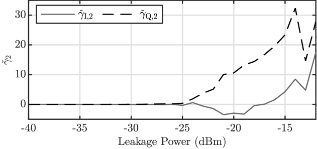
(c)

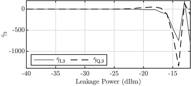
Figure 5: Input-referred coefficients of intermodulation products in RF receiver: (a) IMD2, (b) IMD4 and (c) IMD6.

Fig. 5 depicts the real and imaginary parts of the input-referred coefficients ${\check{\gamma}_{k}=\gamma_{k}/A_{\text{lin}}}$, which differ considerably. The values are not constant, since for low input power levels, the IMD products are below the noise floor, thereby increasing the error of the fit. Additionally, for high input powers, compression effects occur that are not covered by the IMD modeling provided in Section II.

In addition to the receiver nonlinearity, we take the Tx distortions caused by the PA into account. This is achieved by replacing the ideal Tx RF model (1) by

$$x_{\text{RF}}(t)=\Re\left\{g_{\text{BB}}^{\text{PA}}(x_{\text{BB}}(t))\,e^{j2\pi f_{\text{Tx}}t}\right\}$$ (69)

with the equivalent BB transfer characteristic $g_{\text{BB}}^{\text{PA}}(.)$ of the PA. With this model, we assume that the power of any harmonic emissions caused by the PA is much lower than the in-band signal power. For $g_{\text{BB}}^{\text{PA}}(.)$, we choose the well-known Rapp model, which is a memoryless behavioral model for solid-state amplifiers [44, 45]:

$$g_{\text{BB}}^{\text{PA}}(x_{\text{BB}}(t))=\frac{A_{\text{PA}}\left|x_{\text{BB}}(t)\right|}{\left(1+\left(\frac{A_{\text{PA}}\left|x_{\text{BB}}(t)\right|}{x_{\text{max}}}\right)^{2p}\right)^{\frac{1}{2p}}}\,e^{j\arg(x_{\text{BB}}(t))}.$$ (70)

This model describes the nonlinear AM-AM conversion by means of a smooth saturation characteristic, while assuming that the AM-PM conversion is neglible. The smoothness of the transition from the linear part to the saturation region is given by the parameter $p$, the output saturation level is specified by $x_{\text{max}}$. In the following simulations, $A_{\text{PA}}$ is varied to reflect different interference power levels. Thus, instead of using an absolute value for $x_{\text{max}}$, we define it implicitly by means of the CR

$$\text{CR}=20\log_{10}\frac{x_{\text{max}}}{A_{\text{PA}}\sigma_{x}}.$$ (71)

$\sigma_{x}$ is the RMS value of $x_{\text{BB}}(t)$. We approximate the behavior of the discrete PA in our measurement setup with the parameters ${p=2}$ and ${\text{CR}=$6\text{\,}\mathrm{dB}\text{/}$}$.

The leakage path $\tilde{h}_{\text{BB}}^{\text{TxL}}[n]$ is modeled by means of fitted FIR impulse responses, which are based on the measured duplexer stop-band frequency responses. All impulse responses contain 21 values, which decay towards higher delays. The Tx-Rx isolation is about $50\text{\,}\mathrm{dB}\text{/}$.

The Tx signal is an LTE-20 UL signal with a 16-QAM alphabet and 10 RB allocated in the index range $[10,19]$, where the index 1 is at the lower end of the BB spectrum. The Rx signal is chosen to be a fully allocated LTE-20 DL signal, which corresponds to a utilized bandwidth of $18\text{\,}\mathrm{MHz}\text{/}$. Note that LTE-20 is used due to limitations of the RF setup. Clearly, the proposed algorithms are applicable to the higher bandwidths defined by the 5G standard, too. The power of the Rx signal at the chip input is $-72\text{\,}\mathrm{dBm}\text{/}$, which is close to reference sensitivity [46] at the input of the external LNA. The SNR without IMD is about $10\text{\,}\mathrm{dB}\text{/}$.

In all scenarios, the DSIM is applied before the CSF. For a successful interference cancellation, a correct time-alignment between the Tx and the total Rx signal has to be ensured. In an online operation, this could be achieved by applying a correlation-based adaptive synchronization on the strongest IMD component [47] or by utilizing a known constant delay. Using the described parameters, exemplary signals are generated in a simulation based on (12) and the average cancellation performance is computed. This evaluation approach is vital especially for LMS-type algorithms, since they typically suffer from a high performance spread. In the simulation, we neglect any intermodulation products between the leakage signal, the wanted Rx signal and noise due to the wide bandwidth and low power of the wanted and noise components. Even if this assumption was not fulfilled, our simplification would only affect the optimum SNR, but not the relative performance between several DSIM algorithms. Due to the narrow allocation, no oversampling is required for the analyzed IMD products, i. e. up to the sixth order.

V-B Scaled Nonlinearity in Q-Path

In the first test case, we assume a scalar coupling between the nonlinearities in the I- and Q-path. While this assumption is not fulfilled by the targeted receiver, it enables a comparison between the CI-WSAF and the comparably low-complex IM2LMS. In addition, we include the computationally intensive, but very general, KRLS algorithm. Since the ratio between the measured coefficients $\gamma_{k,\text{I}}$ and $\gamma_{k,\text{Q}}$ changes substantially over the leakage power range, we alter these values for this simulation. We keep the interference power unchanged and assume a coupling of ${\delta_{\text{Q}}=-1}$, leading to the modified coefficients

$$\tilde{\gamma}_{k}=(1-j)\,\frac{\operatorname{sgn}(\gamma_{k,\text{I}})\left|\gamma_{k}\right|}{\sqrt{2}}.$$ (72)

The value of $\delta_{\text{Q}}$ does not influence the performance, since it is reliably estimated by the single-tap scaler.

The cancellation performance of the algorithms is compared by means of the SINR

$$\text{SINR}\coloneqq\frac{\operatorname{\mathrm{E}}\left[\left|\check{y}_{\text{BB}}^{\text{Rx}}[n]\right|^{2}\right]}{\operatorname{\mathrm{E}}\left[\left|y_{\text{BB}}^{\text{IMD}}[n]-\hat{y}_{\text{BB}}^{\text{IMD}}[n]+\check{\eta}_{\text{BB}}[n]\right|^{2}\right]},$$ (73)

which is averaged over two LTE slots, while excluding the first symbol. Thus, the initial convergence does not affect the measured performance.

Figure 6: Steady-state SINR improvement for various IMD cancellation schemes in case of scaled nonlinearity in Q-path.

Fig. 6 depicts the SINR for two variants of the CI-WSAF and two algorithms for comparison. In addition, we show the impact of the PA model. Each value is the ensemble average over the results for six different fitted duplexer impulse responses, where for each duplexer 50 runs with randomly generated signals were performed. The linear filter length of all algorithms is set to 16. All relevant parameters are optimized for the individual leakage power levels to guarantee the highest possible performance for a fair comparison. In case of the IM2LMS, previous knowledge about the sign of the real part of the IMD2 component is required in order to ensure correct operation. In practice, this information could be obtained by correlating $\left|x_{\text{BB}}[n]\right|^{2}$ with $y_{\text{BB}}^{\text{Tot}}[n]$. Since the output of the IM2LMS is real-valued, the Q-path interference is estimated using (50), similar to the CI-WSAF. Because of its superior performance, we employ the weighted LS solution with ${\lambda_{\text{cpl}}=0.9998}$ for this purpose. The DC cancellation in the receiver is replicated by applying the notch filter ${H(z)=(1\!-\!z^{-1})/(1\!-\!0.998z^{-1})}$ to the IM2LMS output. The step-size of the IM2LMS is selected in the range $(0,0.056]$, where extremely small values are used for low interference powers. The regularization parameter is chosen within $[0.01,1]$. Despite the necessity of prior knowledge, the IM2LMS shows the lowest SINR among the compared algorithms. The CI-WSAF is used in the TD variant (55) with the norm limiting (56). In order to improve the adaptation rate of the spline-based algorithm, the weights of the linear section are initialized to random constants, which are unaltered for all runs. The fixed nonlinearity is ${\zeta(s)=|s|^{2}}$ to avoid a square root in the feedback loop.

TABLE V: Parameter values of CI-WSAF for IMD cancellation.

Parameter	Value(s)	Parameter	Value(s)
$Q_{\text{lin}}$	$16$	$\tau$	$[1,660]$
$\mathbf{w}[0]$	$\sim\mathcal{N}_{Q_{\text{lin}}}(\mathbf{0},0.01\,\mathbf{I})$	$N_{\text{sp}}$	$20$
$p$	1	$Q_{\text{sp}}$	$3$, $4$
$\rho_{w}$	3	$r_{0}$	$-0.1$, $-0.15$
$\mu$	$[0.0015,0.015]$	$\Delta r$	$0.05$
$\xi$	$[0.0023,0.45]$

Table V summarizes the chosen parameter ranges for the CI-WSAF, where most values tend to become larger with increasing leakage power. $\mathcal{N}_{Q_{\text{lin}}}$ denotes a multivariate normal distribution. The parameter $\lambda_{\text{cpl}}$ of the single-tap scaler was again $0.9998$. A negative value for the first knot $r_{0}$ enables a domain of the spline function down to 0, as required by the fixed nonlinearity $|s|^{2}$. We have ${h_{\text{out}}[n]=1}$, since we do not employ any pipelining and the cancellation is performed before the CSF. In Fig. 6, the CI-WSAF shows excellent performance, clearly outperforming the IM2LMS by up to $12.5\text{\,}\mathrm{dB}\text{/}$. For all leakage powers levels, it restores the SINR to values above the $0\text{\,}\mathrm{dB}\text{/}$ threshold. For the same number of control points, there is no benefit of using cubic CR-splines instead of quadratic B-splines, likely due to the smoothness of the IMD nonlinearity. Compared to a linear PA model, the clipping of the signals peaks by the Rapp PA model slightly improves the performance of the WSAF algorithms. Without clipping, signal peaks occur very seldomly, leading to slow adaptation of the corresponding spline control points and, in further consequence, higher estimation errors. Another minor SINR improvement is achievable by using an LS-based learning algorithm, in our case the KRLS. For this simulation, we used a complexified Gaussian kernel with a standard deviation in the range ${[5,100]}$. The dictionary size was limited by means of the ALD approach with a threshold in the range ${[10^{-5},5\cdot 10^{-5}]}$. Due to its fast convergence and high complexity, the KRLS weights were adapted for the first three LTE symbols, or about 6600 samples, only. Its maximum SINR advantage over the CI-WSAF is about $1\text{\,}\mathrm{dB}\text{/}$. A practical aspect to improve the convergence of all algorithms is to disable the adaption for all samples close to the symbol boundaries within $x_{\text{BB}}[n]$. This measure avoids high error values, which would be caused by the bandwidth increase at symbol transitions [39].

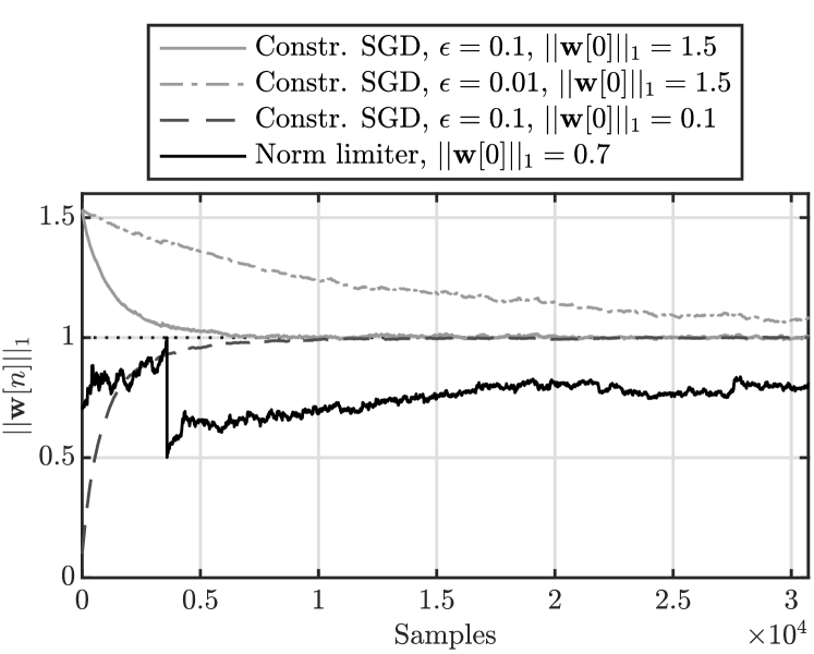
Figure 7: Adaptation of $\ell_{1}$ norm of filter weights due to constrained SGD optimization and limiter.

Another interesting aspect of the CI-WSAF is the constraint on the filter weights, which helps to avoid internal clipping. In Fig. 7, the evolution of the $\ell_{1}$ norm of $\mathbf{w}[n]$ is compared for a leakage power of $-18\text{\,}\mathrm{dBm}\text{/}$ and different parameters of the constraint. Using the constrained SGD method with a weighting of ${\epsilon=0.1}$, $\left\lVert\mathbf{w}[n]\right\rVert_{1}$ convergences close to the desired value of 1 within three symbols. A weighting of ${\epsilon=0.01}$ already slows down the adaptation substantially, but still the norm tends towards 1, thereby reducing the clipping. Although this method shows the expected results, the second optimization goal potentially impacts the steady-state interference cancellation by slowing down the overall adaptation. In contrast, the norm limiting is also able to reduce clipping while not impacting the steady-state performance at all. However, the weight rescaling in the initial phase leads to a performance disadvantage in the first 5000 samples.

V-C Independent Nonlinearity in I- and Q-Path

In the second major test case, we allow for independent coefficients $\gamma_{k,\text{I}}$ and $\gamma_{k,\text{Q}}$, a requirement indicated by measurements on the test receiver. The IM2LMS and the CI-WSAF are not suitable for this scenario, thus, we resort to a comparison between the CIO-WSAF and the KRLS.

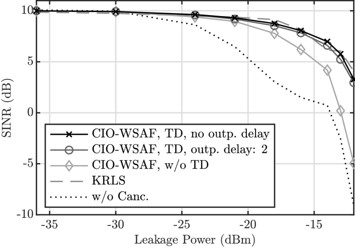
Figure 8: Steady-state SINR improvement for general IMD problem with independent nonlinearities in I- and Q-path.

The first metric we analyze is again the SINR, depicted in Fig. 8. The overall SINR degradation without any countermeasures is similar to the previous section, but now the underlying number of parameters is higher. Interestingly, this causes the previous small performance advantage of the KRLS to vanish completely. Again, its kernel standard deviation was chosen in the range $[4.8,141]$, whereas the ALD threshold was chosen within $[10^{-5},5\cdot 10^{-5}]$. The KRLS weights and the dictionary were adapted for the first three LTE symbols. Unlike the KRLS, the CIO-WSAF with transformed input exhibits a slight SINR improvement compared to the CI-WSAF. The simulation shows that the approximated step-size normalization of the CIO-WSAF behaves just as the standard version used in the CI-WSAF. Compared to Table V, the step-size ${\mu\in[4.4\cdot 10^{-4},0.025]}$, the coupling factor ${\tau\in[1.3,1200]}$ and the regularization ${\xi\in[0.017,0.16]}$ required readjustments. The other parameters could be reused. Since no output filter is present, we have ${h_{\text{g}}=1}$ and ${k_{\text{g}}=0}$. We only consider quadratic interpolation, thus, $Q_{\text{sp}}=3$. In Fig. 8, we included two other variants of the CIO-WSAF. One incorporates a delay of two samples in the output signal, possibly caused by pipelining stages in the design. In the algorithm, this configuration requires ${k_{\text{g}}=2}$. The performance cost of this measure is minor, supporting a real-time implementation of our approach. The second WSAF variant we included does not use a transformed input vector for the linear section and has no output delay (i. e. ${k_{\text{g}}=0}$). Due to the properties of the LTE UL signal, which acts as a reference, the omission of the approximate decorrelation leads to SINR drop of up to $8.2\text{\,}\mathrm{dB}\text{/}$.

Figure 9: PSD of important Rx signal components before and after IMD cancellation using CIO-WSAF.

In addition to the integral performance quantified by the SINR, the PSD of the Rx signal components in Fig. 9 gives a descriptive visualization of the cancellation process. As a baseline, we show the noise floor $\check{\eta}_{\text{BB}}[n]$ and the ideal Rx signal $\check{y}_{\text{BB}}^{\text{Rx}}[n]$, which, combined with the IMD interference, form the total Rx signal $y_{\text{BB}}^{\text{Tot}}[n]$. In this example, we chose a leakage power of $-14\text{\,}\mathrm{dBm}\text{/}$. For interference cancellation, we apply the CIO-WSAF with transformed input and no pipelining, which generates the interference replica $\hat{y}_{\text{BB}}^{\text{IMD}}[n]$. After DSIM, the remaining interference ${e_{\text{BB}}^{\text{IMD}}[n]=y_{\text{BB}}^{\text{IMD}}[n]-\hat{y}_{\text{BB}}^{\text{IMD}}[n]}$ is below the Rx level, which acts as additional noise from the perspective of the CIO-WSAF. The signal after DSIM, $y_{\text{BB}}^{\text{Canc}}[n]$, closely resembles the wanted Rx signal. This indicates a successful cancellation, which agrees with the SINR of $7\text{\,}\mathrm{dB}\text{/}$ shown in Fig. 8.

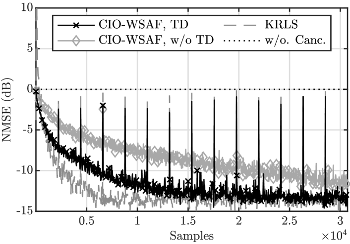
Figure 10: Adaptation behavior of IMD cancellation schemes in case of independent nonlinearities in I- and Q-path.

Another important metric for DSIM applications is the adaptation time of the estimation algorithm. Therefore, in Fig. 10 we compare the NMSE

$$\text{NMSE}[n]\coloneqq\frac{\operatorname{\mathrm{E}}\left[\left|y_{\text{BB}}^{\text{IMD}}[n]-\hat{y}_{\text{BB}}^{\text{IMD}}[n]\right|^{2}\right]}{\operatorname{\mathrm{E}}\left[\left|y_{\text{BB}}^{\text{IMD}}[n]\right|^{2}\right]}$$ (74)

for two SAF variants and the KRLS at a leakage power level of $-18\text{\,}\mathrm{dBm}\text{/}$. As expected for RLS-type algorithms, the KRLS features very fast adaptation within the training sequence of $6600$ samples. In contrast, the CIO-WSAF without an input transform requires more than $3\cdot 10^{4}$ samples to reach steady-state. The TD variant manages to reduce the adaptation time to about ${2\cdot 10^{4}}$ samples, which is a remarkable improvement for an SGD algorithm.

VI Conclusion

We presented two novel adaptive learning schemes based on spline interpolation that allow for low-complex digital cancellation of transceiver self-interference caused by higher-order IMD. Based on a comprehensive modeling of the receiver nonlinearities, we derived the BB interference model, allowing to extract a Wiener structure suitable for online estimation. We proposed several extensions to the spline-based algorithm and precisely assessed the computational complexity of all modules. The interference cancellation performance was evaluated in practically relevant IMD scenarios, which were based on measured receiver parameters. Compared to a general nonlinear estimation approach, our algorithms showed similar accuracy at a fraction of the computational costs.

References

- [1] B. Razavi, “Design considerations for direct-conversion receivers,” IEEE Transactions on Circuits and Systems II: Analog and Digital Signal Processing, vol. 44, no. 6, pp. 428–435, Jun. 1997.
- [2] “Saw duplexer, LTE / WCDMA band 3, series: B8625,” TDK, data sheet. [Online]. Available: http://static6.arrow.com/aropdfconversion/d02a7e8b179789d6426087c1ffa6fa33cd180f0f/b8625.pdf
- [3] S. Sadjina, C. Motz, T. Paireder, M. Huemer, and H. Pretl, “A survey of self-interference in LTE-Advanced and 5G New Radio wireless transceivers,” IEEE Transactions on Microwave Theory and Techniques, vol. 68, no. 3, pp. 1118–1131, Feb. 2020.
- [4] A. Frotzscher and G. Fettweis, “Least squares estimation for the digital compensation of Tx leakage in zero-IF receivers,” in 2009 IEEE Global Telecommunications Conference (GLOBECOM), Nov. 2009, pp. 1–6.
- [5] A. Kiayani, L. Anttila, M. Kosunen, K. Stadius, J. Ryynänen, and M. Valkama, “Modeling and joint mitigation of TX and RX nonlinearity-induced receiver desensitization,” IEEE Transactions on Microwave Theory and Techniques, vol. 65, no. 7, pp. 2427–2442, Jul. 2017.
- [6] A. Gebhard, C. Motz, R. S. Kanumalli, H. Pretl, and M. Huemer, “Nonlinear least-mean-squares type algorithm for second-order interference cancellation in LTE-A RF transceivers,” in 2017 51st Asilomar Conference on Signals, Systems, and Computers, 2017, pp. 802–807.
- [7] A. Gebhard, O. Lang, M. Lunglmayr, C. Motz, R. S. Kanumalli, C. Auer, T. Paireder, M. Wagner, H. Pretl, and M. Huemer, “A robust nonlinear RLS type adaptive filter for second-order-intermodulation distortion cancellation in FDD LTE and 5G direct conversion transceivers,” IEEE Transactions on Microwave Theory and Techniques, vol. 67, no. 5, pp. 1946–1961, May 2019.
- [8] A. Frotzscher and G. Fettweis, “A stochastic gradient LMS algorithm for digital compensation of Tx leakage in zero-IF-receivers,” in 2008 IEEE Vehicular Technology Conference (VTC Spring), May 2008, pp. 1067–1071.
- [9] C. Lederer and M. Huemer, “LMS based digital cancellation of second-order TX intermodulation products in homodyne receivers,” in 2011 IEEE Radio and Wireless Symposium, Jan. 2011, pp. 207–210.
- [10] E. A. Keehr and A. Hajimiri, “Successive regeneration and adaptive cancellation of higher order intermodulation products in RF receivers,” IEEE Transactions on Microwave Theory and Techniques, vol. 59, no. 5, pp. 1379–1396, May 2011.
- [11] T. Paireder, C. Motz, S. Sadjina, and M. Huemer, “A robust mixed-signal cancellation approach for even-order intermodulation distortions in LTE-A/5G-transceivers,” IEEE Transactions on Circuits and Systems II: Express Briefs, vol. 68, no. 3, pp. 923–927, Mar. 2021.
- [12] D. Comminiello and J. Principe, Eds., Adaptive Learning Methods for Nonlinear System Modeling. Elsevier Science, 2018.
- [13] C. Auer, K. Kostoglou, T. Paireder, O. Ploder, and M. Huemer, “Support vector machines for self-interference cancellation in mobile communication transceivers,” in 2020 IEEE 91st Vehicular Technology Conference (VTC2020-Spring), 2020, pp. 1–6.
- [14] C. Auer, T. Paireder, O. Lang, and M. Huemer, “Kernel recursive least squares based cancellation for receiver-induced self-interference,” in 2020 54th Asilomar Conference on Signals, Systems, and Computers, 2020, accepted for publication.
- [15] L. Vecci, F. Piazza, and A. Uncini, “Learning and approximation capabilities of adaptive spline activation function neural networks,” Neural Networks, vol. 11, no. 2, pp. 259–270, 1998.
- [16] A. Uncini and F. Piazza, “Blind signal processing by complex domain adaptive spline neural networks,” IEEE Transactions on Neural Networks, vol. 14, no. 2, pp. 399–412, 2003.
- [17] P. Bohra, J. Campos, H. Gupta, S. Aziznejad, and M. Unser, “Learning activation functions in deep (spline) neural networks,” IEEE Open Journal of Signal Processing, vol. 1, pp. 295–309, 2020.
- [18] D. Comminiello, M. Scarpiniti, L. A. Azpicueta-Ruiz, J. Arenas-García, and A. Uncini, “Functional link adaptive filters for nonlinear acoustic echo cancellation,” IEEE Transactions on Audio, Speech, and Language Processing, vol. 21, no. 7, pp. 1502–1512, 2013.
- [19] M. Scarpiniti, D. Comminiello, R. Parisi, and A. Uncini, “Nonlinear spline adaptive filtering,” Signal Processing, vol. 93, no. 4, p. 772–783, Apr. 2013.
- [20] ——, “Hammerstein uniform cubic spline adaptive filters: Learning and convergence properties,” Signal Processing, vol. 100, p. 112–123, Jul. 2014.
- [21] M. Scarpiniti, D. Comminiello, R. Parisi, and A. Uncini, “Novel cascade spline architectures for the identification of nonlinear systems,” IEEE Transactions on Circuits and Systems I: Regular Papers, vol. 62, no. 7, pp. 1825–1835, Jun. 2015.
- [22] P. P. Campo, D. Korpi, L. Anttila, and M. Valkama, “Nonlinear digital cancellation in full-duplex devices using spline-based hammerstein model,” in 2018 IEEE Globecom Workshops (GC Wkshps), 2018, pp. 1–7.
- [23] P. Pascual Campo, L. Anttila, D. Korpi, and M. Valkama, “Cascaded spline-based models for complex nonlinear systems: Methods and applications,” IEEE Transactions on Signal Processing, vol. 69, pp. 370–384, Dec. 2020.
- [24] A. Gebhard, “Self-interference cancellation and rejection in FDD RF-transceivers,” Ph.D. dissertation, Johannes Kepler University Linz, 2019.
- [25] E. Ahmed, A. M. Eltawil, and A. Sabharwal, “Self-interference cancellation with nonlinear distortion suppression for full-duplex systems,” in 2013 Asilomar Conference on Signals, Systems and Computers, 2013, pp. 1199–1203.
- [26] C. Mollén, U. Gustavsson, T. Eriksson, and E. G. Larsson, “Impact of spatial filtering on distortion from low-noise amplifiers in massive MIMO base stations,” IEEE Transactions on Communications, vol. 66, no. 12, pp. 6050–6067, 2018.
- [27] C. Motz, T. Paireder, and M. Huemer, “Modulated spur interference cancellation for LTE-A/5G transceivers: A system level analysis,” in 2020 IEEE 91st Vehicular Technology Conference (VTC Spring), May 2020.
- [28] J. F. Epperson, “On the runge example,” The American Mathematical Monthly, vol. 94, no. 4, pp. 329–341, 1987.
- [29] C. de Boor, A Practical Guide to Splines. Springer New York, 2001, revised ed.
- [30] L. Schumaker, Spline Functions: Basic Theory, 3rd ed., ser. Cambridge Mathematical Library. Cambridge University Press, 2007.
- [31] E. Catmull and R. Rom, “A class of local interpolating splines,” in Computer Aided Geometric Design, R. E. Barnhill and R. F. Riesenfeld, Eds. Academic Press, 1974, pp. 317 – 326.
- [32] Y. Gu, J. Jin, and S. Mei, “ norm constraint LMS algorithm for sparse system identification,” IEEE Signal Processing Letters, vol. 16, no. 9, pp. 774–777, 2009.
- [33] D. C. v. Grünigen, Digitale Signalverarbeitung: mit einer Einführung in die kontinuierlichen Signale und Systeme, 5th ed. Hanser, 2014, (in German).
- [34] P. Dhrymes, Mathematics for Econometrics, 4th ed. Springer New York, 2013.
- [35] R. Remmert and R. Burckel, Theory of Complex Functions, ser. Graduate Texts in Mathematics. Springer New York, 1991.
- [36] D. H. Brandwood, “A complex gradient operator and its application in adaptive array theory,” IEE Proceedings F - Communications, Radar and Signal Processing, vol. 130, no. 1, pp. 11–16, Feb. 1983.
- [37] A. I. Hanna and D. P. Mandic, “A fully adaptive normalized nonlinear gradient descent algorithm for complex-valued nonlinear adaptive filters,” IEEE Transactions on Signal Processing, vol. 51, no. 10, pp. 2540–2549, 2003.
- [38] P. S. Diniz, Adaptive Filtering: Algorithms and Practical Implementation, 2nd ed. Kluwer Academic Publishers, 2002.
- [39] C. Motz, T. Paireder, and M. Huemer, “Improving digital interference cancellation in LTE-A/5G-transceivers by statistical modeling,” in 2020 54th Asilomar Conference on Signals, Systems, and Computers, 2020, accepted for publication.
- [40] S. F. Obermann and M. J. Flynn, “Division algorithms and implementations,” IEEE Transactions on Computers, vol. 46, no. 8, pp. 833–854, Aug. 1997.
- [41] V. Kober, “Fast algorithms for the computation of sliding discrete sinusoidal transforms,” IEEE Transactions on Signal Processing, vol. 52, no. 6, pp. 1704–1710, Jun. 2004.
- [42] Y. Engel, S. Mannor, and R. Meir, “The kernel recursive least-squares algorithm,” IEEE Transactions on Signal Processing, vol. 52, no. 8, pp. 2275–2285, Jul. 2004.
- [43] R. Boloix-Tortosa, J. J. Murillo-Fuentes, and S. A. Tsaftaris, “The generalized complex kernel least-mean-square algorithm,” IEEE Transactions on Signal Processing, vol. 67, no. 20, pp. 5213–5222, 2019.
- [44] S. Glock, J. Rascher, B. Sogl, T. Ussmueller, J. Mueller, and R. Weigel, “A memoryless semi-physical power amplifier behavioral model based on the correlation between AM–AM and AM–PM distortions,” IEEE Transactions on Microwave Theory and Techniques, vol. 63, no. 6, pp. 1826–1835, 2015.
- [45] C. Rapp, “Effects of HPA-nonlinearity on a 4-DPSK/OFDM-signal for a digital sound broadcasting signal,” ESA Special Publication, vol. 332, pp. 179–184, 1991.
- [46] 3GPP, “Evolved Universal Terrestrial Radio Access (E-UTRA); Physical channels and modulation,” 3rd Generation Partnership Project (3GPP), Technical Specification (TS) 36.211, 04 2017, version 14.2.0.
- [47] T. Paireder, C. Motz, O. Lang, and M. Huemer, “Time-delay estimation for self-interference cancellation in LTE-A/5G transceivers,” in 2019 Austrochip Workshop on Microelectronics (Austrochip), 2019, pp. 21–28.