A Greedy Algorithm for Quantizing Neural Networks
Abstract
We propose a new computationally efficient method for quantizing the weights of pre-trained neural networks that is general enough to handle both multi-layer perceptrons and convolutional neural networks. Our method deterministically quantizes layers in an iterative fashion with no complicated re-training required. Specifically, we quantize each neuron, or hidden unit, using a greedy path-following algorithm. This simple algorithm is equivalent to running a dynamical system, which we prove is stable for quantizing a single-layer neural network (or, alternatively, for quantizing the first layer of a multi-layer network) when the training data are Gaussian. We show that under these assumptions, the quantization error decays with the width of the layer, i.e., its level of over-parametrization. We provide numerical experiments, on multi-layer networks, to illustrate the performance of our methods on MNIST and CIFAR10 data, as well as for quantizing the VGG16 network using ImageNet data.
Keywords: quantization, neural networks, deep learning, stochastic control, discrepancy theory
1 Introduction
Deep neural networks have taken the world by storm. They outperform competing algorithms on applications ranging from speech recognition and translation to autonomous vehicles and even games, where they have beaten the best human players at, e.g., Go (see, LeCun et al. 2015; Goodfellow et al. 2016; Schmidhuber 2015; Silver et al. 2016). Such spectacular performance comes at a cost. Deep neural networks require a lot of computational power to train, memory to store, and power to run (e.g., Han et al. 2016; Kim et al. 2016; Gupta et al. 2015; Courbariaux et al. 2015). They are painstakingly trained on powerful computing devices and then either run on these powerful devices or on the cloud. Indeed, it is well-known that the expressivity of a network depends on its architecture (Baldi and Vershynin, 2019). Larger networks can capture more complex behavior (Cybenko, 1989) and therefore, for example, they generally learn better classifiers. The trade off, of course, is that larger networks require more memory for storage as well as more power to run computations. Those who design neural networks for the purpose of loading them onto a particular device must therefore account for the device’s memory capacity, processing power, and power consumption. A deep neural network might yield a more accurate classifier, but it may require too much power to be run often without draining a device’s battery. On the other hand, there is much to be gained in building networks directly into hardware, for example as speech recognition or translation chips on mobile or handheld devices or hearing aids. Such mobile applications also impose restrictions on the amount of memory a neural network can use as well as its power consumption.
This tension between network expressivity and the cost of computation has naturally posed the question of whether neural networks can be compressed without compromising their performance. Given that neural networks require computing many matrix-vector multiplications, arguably one of the most impactful changes would be to quantize the weights in the neural network. In the extreme case, replacing each -bit floating point weight with a single bit would reduce the memory required for storing a network by a factor of and simplify scalar multiplications in the matrix-vector product. It is not clear at first glance, however, that there even exists a procedure for quantizing the weights that does not dramatically affect the network’s performance.
1.1 Contributions
The goal of this paper is to propose a framework for quantizing neural networks without sacrificing their predictive power, and to provide theoretical justification for our framework. Specifically,
-
•
We propose a novel algorithm in (4) and (4) for sequentially quantizing layers of a pre-trained neural network in a data-dependent manner. This algorithm requires no retraining of the network, requires tuning only hyperparameters—namely, the number of bits used to represent a weight and the radius of the quantization alphabet—and has a run time complexity of operations per layer. Here, is the ambient dimension of the inputs, or equivalently, the number of features per input sample of the layer, while is the number of training samples used to learn the quantization. This bound is optimal in the sense that any data-dependent quantization algorithm requires reading the entries of the training data matrix. Furthermore, this algorithm is parallelizable across neurons in a given layer.
-
•
We establish upper bounds on the relative training error in Theorem 2 and the generalization error in Theorem 3 when quantizing the first layer of a neural network that hold with high probability when the training data are Gaussian. Additionally, these bounds make explicit how the relative training error and generalization error decay as a function of the overparametrization of the data.
-
•
We provide numerical simulations in Section 6 for quantizing networks trained on the benchmark data sets MNIST and CIFAR10 using both multilayer perceptrons and convolutional neural networks. We quantize all layers of the neural networks in these numerical simulations to demonstrate that the quantized networks generalize very well even when the data are not Gaussian.
2 Notation
Throughout the paper, we will use the following notation. Universal constants will be denoted as and their values may change from line to line. For real valued quantities , we write when we mean that and when we mean . For any natural number , we denote the set by . For column vectors , the Euclidean inner product is denoted by , the -norm by , the -norm by , and the -norm by . will denote the -ball centered at with radius and we will use the notation . For a sequence of vectors with , the backwards difference operator acts by . For a matrix we will denote the rows using lowercase characters and the columns with uppercase characters . For two matrices we denote the Frobenius norm by . will denote a -layer neural network, or multilayer perceptron, which acts on data via
Here, is a rectifier which acts on each component of a vector, is an affine operator with and is the layer’s weight matrix, is the bias.
3 Background
While there are a handful of empirical studies on quantizing neural networks, the mathematical literature on the subject is still in its infancy. In practice there appear to be three different paradigms for quantizing neural networks. These include quantizing the gradients during training, quantizing the activation functions, and quantizing the weights either during or after training. Guo (2018) presents an overview of these different paradigms. Any quantization that occurs during training introduces issues regarding the convergence of the learning algorithm. In the case of using quantized gradients, it is important to choose an appropriate codebook for the gradient prior to training to ensure stochastic gradient descent converges to a local minimum. When using quantized activation functions, one must suitably modify backpropagation since the activation functions are no longer differentiable. Further, enforcing the weights to be discrete during training also causes problems for backpropagation which assumes no such restriction. In any of these cases, it will be necessary to carefully choose hyperparameters and modify the training algorithm beyond what is necessary to train unquantized neural networks. In contrast to these approaches, our result allows the practitioner to train neural networks in any fashion they choose and quantizes the trained network afterwards. Our quantization algorithm only requires tuning the number of bits that are used to represent a weight and the radius of the quantization alphabet. We now turn to surveying approaches similar to ours which quantize weights after training.
A natural question to ask is whether or not for every neural network there exists a quantized representation that approximates it well on a given data set. It turns out that a partial answer to this question lies in the field of discrepancy theory. Ignoring bias terms for now, let’s look at quantizing the first layer. There we have some weight matrix which acts on input by and this quantity is then fed through the rectifier. Of course, a layer can act on a collection of inputs stored as the rows in a matrix where now the rectifier acts componentwise. Focusing on just one neuron , or column of , rather than viewing the matrix vector product as a collection of inner products , we can think about this as a linear combination of the columns of , namely . This elementary linear algebra observation now lends the quantization problem a rather elegant interpretation: is there some way of choosing quantized weights from a fixed alphabet , such as , so that the walk approximates the walk ?
As we mentioned above, the study of the existence of such a when has a rather rich history from the discrepancy theory literature. Spencer (1985) in Corollary 18 was able to prove the following surprising claim. There exists an absolute constant so that given vectors with there exists a vector so that . What makes this so remarkable is that the upper bound is independent of , or the number of vectors in the walk. Spencer further remarks that János Komlós has conjectured that this upper bound can be reduced to simply . The proof of the Komlós conjecture seems to be elusive except in special cases. One special case where it is true is if we require and now allow . Theorem 16 in Spencer (1985) then proves that there exists universal constants and so that for every collection of vetors with there is some with and .
Spencer’s result inspired others to attack the Komlós conjecture and variants thereof. Banaszczyk (1990) was able to prove a variant of Spencer’s result for vectors chosen from an ellipsoid. In the special case where the ellipsoid is the unit ball in , Banaszczyk’s result says for any there exists so that . This bound is tight, as it is achieved by the walk with and when the vectors form an orthonormal basis. Later works consider a more general notion of boundedness. Rather than controlling the infinity or Euclidean norm one might instead wonder if there exists a bit string so that the quantized walk never leaves a sufficiently large convex set containing the origin. The first such result, to the best of our knowledge, was proven by Giannopoulos (1997). Giannopoulos proved there that for any origin-symmetric convex set with standard Gaussian measure and for any collection of vectors there exists a bit string so that . Notice here that the number of vectors in this result is equal to the dimension. Banaszczyk (1998) strengthened this result by allowing the number of vectors to be arbitrary and further showed that, under the same assumption , there exists a which satisfies . Scaling the hypercube appropriately, this immediately implies that the bound in Spencer’s result can be reduced from to . Though the above results were formulated in the special case when , a result by Lovasz et al. (1986) proves that results in this special case naturally extend to results in the linear discrepancy case when , though the universal constant scales by a factor of 2.
While all of these works are important contributions towards resolving the Komlós conjecture, many important questions remain, particularly pertaining to their applicability to our problem of quantizing neural networks. Naturally the most important question remains on how to construct such a given , . A naïve first guess towards answering both questions would be to solve an integer least squares problem. That is, given a data set a neuron , and a quantization alphabet , such as {-1, 1}, solve
| (1) | ||||||
| subject to |
It is well-known, however, that solving (1) is NP-Hard. See, for example, Ajtai (1998). Nevertheless, there have been many iterative constructions of vectors which satisfy the bounds in the aforementioned works. A non-comprehensive list of such works includes Bansal (2010); Lovett and Meka (2015); Rothvoss (2017); Harvey et al. (2014); Eldan and Singh (2014). Constructions of which satisfy the bound in the result of Banaszczyk (1998) include the works of Dadush et al. (2016); Bansal et al. (2018). These works also generalize to the linear discrepancy setting. In fact, Bansal et al. (2018) prove a much more general result which allows the use of more arbitrary alphabets other than . Their algorithm is random though, so their result holds with high probability on the execution of the algorithm. This is in contrast, as we will see, with our result which will hold with high probability on the draw of Gaussian data. Beyond this, the computational complexity of the algorithms in Dadush et al. (2016); Bansal et al. (2018) prohibit their use in quantizing deep neural networks. For Dadush et al. (2016), this consists of looping over iterations of solving a semi-definite program and computing a Cholesky factorization for a matrix. The Gram-Schmidt walk algorithm in Bansal et al. (2018) has a run-time complexity of , where is the exponent for matrix multiplication. These complexities are already quite restrictive and only give the run-time for quantizing a single neuron. As the number of neurons in each layer is likely to be large for deep neural networks, these algorithms are simply infeasible for the task at hand. As we will see, our algorithm in comparison has a run-time complexity of per neuron which is optimal in the sense that any data driven approach towards constructing will require one pass over the entries of . Using a norm inequality on Banasczyzk’s bound, the result in Bansal (2010) guarantees for the existence of a such that . Provided is a generic vector in the hypercube, namely that , then a simple calculation shows that with high probability on the draw of Gaussian data with entries having variance to ensure that the columns are approximately unit norm, the Gram-Schmidt walk achieves a relative error bound of . As we will see in Theorem 2, our relative training error bound for quantizing neurons in the first layer decays like . In other words, to achieve a relative error of less than in the overparametrized regime where , the Gram-Schmidt walk requires on the order of floating point operations as compared to our algorithm which only requires on the order of floating point operations.
With no quantization algorithm that is both competitive from a theoretical perspective and computationally feasible, we turn to surveying what has been done outside the mathematical realm. Perhaps the simplest manner of quantizing weights is to quantize each weight within each neuron independently. The authors in Rastegari et al. (2016) consider precisely this set-up in the context of convolutional neural networks (CNNs). For each weight matrix the quantized weight matrix and optimal scaling factor are defined as minimizers of subject to the constraint that for all . It turns out that the analytical solution to this optimization problem is and . This form of quantization has long been known to the digital signal processing community as Memoryless Scalar Quantization (MSQ) because it quantizes a given weight independently of all other weights. While MSQ may minimize the Euclidean distance between two weight matrices, we will see that it is far from optimal if the concern is to design a matrix which approximates on an overparameterized data set. Other related approaches are investigated in, e.g., Hubara et al. (2017).
In a similar vein, Wang and Cheng (2017) consider learning a quantized factorization of the weight matrix , where the matrices are ternary matrices with entries and is a full-precision diagonal matrix. While in general this is a NP-hard problem authors use a greedy approach for constructing inspired by the work of Kolda and O’leary (1998). They provide simulations to demonstrate the efficacy of this method on a few pre-trained models, yet no theoretical analysis is provided for the efficacy of this framework. We would like to remark that the work Kueng and Tropp (2019) gives a framework for computing factorizations of when as , where . The reason this work is intruiging is that it does offer a means for compressing the weight matrix by storing a smaller analog matrix and a binarized matrix though it does not offer nearly as much compression as if we were to replace by a fully quantized matrix . Indeed, the matrix is not guaranteed to be binary or admit a representation with a low-complexity quantization alphabet. Nevertheless, Kueng and Tropp (2019) give conditions under which such a factorization exists and propose an algorithm which provably constructs using semi-definite programming. They extend this analysis to the case when is the sum of a rank matrix and a sparse matrix but do not establish robustness of their factorization to more general noise models.
Extending beyond the case where the quantization alphabet is fixed a priori, Gong et al. (2014) propose learning a codebook through vector quantization to quantize only the dense layers in a convolutional neural network. This stands in contrast to our work where we quantize all layers of a network. They consider clustering weights using -means clustering and using the centroids of the clusters as the quantized weights. Moreover, they consider three different methods of clustering, which include clustering the neurons as vectors, groups of neurons thought of as sub-matrices of the weight matrix, and quantizing the neurons and the successive residuals between the cluster centers and the neurons. Beyond the fact that this work does not consider quantizing the convolutional layers, there is the additional shortcoming that clustering the neurons or groups thereof requires choosing the number of clusters in advance and choosing a maximal number of iterations to stop after. Our algorithm gives explicit control over the alphabet in advance, requires tuning only the radius of the quantization alphabet, and runs in a fixed number of iterations. Similar to the above work, we make special mention of Deep Compression by Han et al. (2016). Deep Compression seems to enjoy compressing large networks like AlexNet without sacrificing their empirical performance on data sets like ImageNet. There, authors consider first pruning the network and quantizing the values of the (scalar-valued) weights in a given layer using -means clustering. This method applies both to fully connected and convolutional layers. An important drawback of this quantization procedure is that the network must be retrained, perhaps multiple times, to fine tune these learned parameters. Once these parameters have been fine tuned, the weight clusters for each layer are further compressed using Huffman coding. We further remark that quantizing in this fashion is sensitive to the initialization of the cluster weights.
4 Algorithm and Intuition
Going forward we will consider neural networks without bias vectors. This assumption may seem restrictive, but in practice one can always use MSQ with a big enough bit budget to control the quantization error for the bias. Even better, one may simply embed the dimensional data/activations and weights into an dimensional space via and so that . In other words, the bias term can simply be treated as an extra dimension to the weight vector, so we will henceforth ignore it. Given a trained neural network with its associated weight matrices and a data set , our goal is to construct quantized weight matrices to form a new neural network for which is small. For simplicity and ease of exposition, we will focus on the extreme case where the weights are constrained to the ternary alphabet , though there is no reason that our methods cannot be applied to arbitrary alphabets.
Our proposed algorithm will quantize a given neuron independently of other neurons. Beyond making the analysis easier this has the practical benefit of allowing us to easily parallelize quantization across neurons in a layer. If we denote a neuron as , we will sucessively quantize the weights in in a greedy data-dependent way. Let be our data matrix, and let denote the analog and quantized neural networks up to layer respectively.
In the first layer, the aim is to achieve by selecting, at the step, so the running sum tracks its analog as well as possible in an sense. That is, at the iteration, we set
It will be more amenable to analysis, and to implementation, to instead consider the equivalent dynamical system where we quantize neurons in the first layer using
| (2) | ||||
One can see, using a simple substitution, that is the error vector at the step. Controlling it will be a main focus in our error analysis. An interesting way of thinking about (4) is by imagining the analog, or unquantized, walk as a drunken walker and the quantized walk is a concerned friend chasing after them. The drunken walker can stumble with step sizes along an avenue in the direction but the friend can only move in steps whose lengths are encoded in the alphabet .
In the subsequent hidden layers, we follow a slightly modified version of (4). Letting , , we quantize neurons in layer by
| (3) | ||||
We say the vector is the quantization of . In this work, we will provide a theoretical analysis for the behavior of (4) and leave analysis of (4) for future work. To that end, we re-emphasize the critical role played by the state variable defined in (4). Indeed, we have the identity . That is, the two neurons act approximately the same on the batch of data only provided the state variable is well-controlled. Given bounded input , systems which admit uniform upper bounds on will be referred to as stable. When the are random, and in our theoretical considerations they will be, we remark that this is a much stronger statement than proving convergence to a limiting distribution which is common, for example, in the Markov chain literature. For a broad survey of such Markov chain techniques, one may consult Meyn and Tweedie (2012). The natural question remains: is the system (4) stable? Before we dive into the machinery of this dynamical system, we would like to remark that there is a concise form solution for . Denote the greedy ternary quantizer by with
Then we have the following.
Lemma 1
In the context of (4), we have for any that
| (4) |
Proof This follows simply by completing a square. Provided , we have by the definition of
Because the former term is always non-negative, it must be the case that the minimizer is .
Any analysis of the stability of (4) must necessarily take into account how the vectors are distributed. Indeed, one can easily cook up examples which give rise to sequences of which diverge rapidly. For the sake of illustration consider restricting our attention to the case when for all . The triangle inequality gives us the crude upper bound
Choosing to minimize , or any -norm for that matter, simply reduces back to the MSQ quantizer where the weights within are quantized independently of one another, namely . It turns out that one can effectively attain this upper bound by adversarially choosing to be orthogonal to for all . Indeed, in that setting we have exactly the MSQ quantizer
Consequentially, by repeatedly appealing to orthogonality,
Thus, for generic vectors , and adversarially chosen , the error scales like . Importantly, this adversarial construction requires knowledge of at “time” , in order to construct an orthogonal . In that sense, this extreme case is rather contrived. In an opposite (but also contrived) extreme case, all of the are equal, and therefore is parallel to for all , the dynamical system reduces to a first order greedy quantizer
| (5) |
Here, when , one can show by induction that for all , a dramatic contrast with the previous scenario. For more details on quantization, see for example Inose et al. (1962); Daubechies and DeVore (2003).
Recall that in the present context the signal we wish to approximate is not the neuron itself, but rather . The goal therefore is not to minimize the error but rather to minimize , which by construction is the same as . Algebraically that means carefully selecting so that is in or very close to the kernel, or null-space, of the data matrix . This immediately suggests how overparameterization may lead to better quantization. Given data samples stored as rows in , having or alternatively having ensures that the kernel of is large, and one may attempt to design so that the vector lies as close as possible to the kernel of .
5 Main Results
We are now ready to state our main result which shows that (4) is stable when the input data are Gaussian. The proofs of the following theorems are deferred to Section 9, as the proofs are quite long and require many supporting lemmata.
Theorem 2
Proof
Without loss of generality, we’ll assume since this factor appears in both numerator and denominator of (6). Theorem 14 guarantees with probability at least that . Using Lemma 8, we have with probability at least . Combining these two results gives us the desired statement.
For generic vectors we have , so in this case Theorem 2 tells us that up to logarithmic factors the relative error decays like . As it stands, this result suggests that it is sufficient to have to obtain a small relative error. In Section 9, we address the case where the feature data lay in a -dimensional subspace to get a bound in terms of rather than . In other words, this suggests that the relative training error depends not on the number of training samples but on the intrinsic dimension of the features . See Lemma 16 for details.
Our next result shows that the quantization error is well-controlled in the span of the training data so that the quantized weights generalize to new data.
Theorem 3
Define and as in the statement of Theorem 2 and further suppose that . Let be the singular value decomposition of , and let where is drawn independently of . In other words, suppose is a Gaussian random variable drawn from the span of the training data . Then with probability at least we have
| (7) |
Proof To begin, notice that the error bound in Theorem 14 easily extends to the set with a simple yet pessimistic argument. With probability at least , for any one has
| (8) |
Now for as defined in the statement of this theorem define , where
If it were the case that then we could use (5) to get the bound
So, it behooves us to find a strictly positive lower bound on . By the assumption that , there exists so that . Since , is injective almost surely and therefore is unique. Setting , observe that and . It follows that . To lower bound , note
| (9) |
The penultimate inequality in the above equation follows directly from well-known bounds on the singular values of isotropic subgaussian matrices that hold with probability at least (see Vershynin 2018). To make the argument explicit, note that , where is a matrix whose rows are independent and identically distributed gaussians with and are thus isotropic. Using Lemma 8 we have with probability at least that . Substituting in (9), we have
Therefore, putting it all together, we have with probability at least
Remark 4
In the special case when , i.e. when and , the bound in Theorem 3 reduces to
Furthermore, when the row data are normalized in expectation, or when , this bound becomes .
Remark 5
Remark 6
The context of Theorem 3 considers the setting when the data are overparameterized, and there are fewer training data points used than the number of parameters. It is natural to wonder if better generalization bounds could be established if many training points were used to learn the quantization. In the extreme setting where , one could use a covering or -net like argument. Specifically, if a new sample were close to a training example , then Such an argument could be done easily when the number of training points is large enough that it leads to a small . On the other hand, the curse of dimensionality stipulates that for this argument to work it would require an exponential number of training points, e.g., of order if the training data were in a -dimensional subspace and did not exhibit any further structure. We choose to focus on the overparametrized setting instead, but think that investigating the “intermediate” setting, where one has more training data coming from a structured -dimensional set than parameters, is an interesting avenue for future work.
Our technique for showing the stability of (4), i.e., the boundedness of , relies on tools from drift analysis. Our analysis is inspired by the works of Pemantle and Rosenthal (1999) and Hajek (1982). Given a real valued stochastic process , those authors give conditions on the increments to uniformly bound the moments, or moment generating function, of the iterates . These bounds can then be transformed into a bound in probability on an individual iterate using Markov’s inequality. Recall that we’re interested in bounding the state variable induced by the system (4) which quantizes the first layer of a neural network. In situations like ours it is natural to analyze the increments of since the innovations are jointly independent. To invoke the results of Pemantle and Rosenthal (1999); Hajek (1982) we’ll consider the associated stochastic process . Beyond the fact that our intent is to control the norm of the state variable, it turns out that stability analyses of vector valued stochastic processes typically involve passing the process through a real-valued and oftentimes quadratic function known as a Lyapunov function. There is a wide variety of stability theorems which require demonstrating certain properties of the image of a stochastic process under a Lyapunov function. For example, Lyapunov functions play a critical role in analyzing Markov chains as detailed in Menshikov et al. (2016). However, there are a few details which preclude us from using one of these well-known stability results for the process . First, even though the innovations are jointly independent the increments
| (10) |
have a dependency structure encoded by the bit sequence . In addition to this, the bigger challenge in the analysis of (4) is the discontinuity inherent in the definition of . Addressing this discontinuity in the analysis requires carefully handling the increments on the events where is fixed.
Based on our prior discussion, towards the end of Section 4, it would seem that for generic data sets the stability of (4) lies somewhere in between the behavior of MSQ and quantizers, and that behavior crucially depends on the “dither” terms . For the sake of analysis then, we will henceforth make the following assumptions.
Assumption 1
The sequence defined on the probability space is adapted to the filtration . Further, all and are jointly independent.
Assumption 2
Assumption 1’s stipulation that the are independent of the weights is a simplifying relaxation, and our proof technique handles the case when the are deterministic. The joint independence of the could be realized by splitting the global population of training data into two populations where one is used to train the analog network and another to train the quantization. In the hypotheses of Theorem 2 it is also assumed that the entries of the weight vector are sufficiently separated from the characters of the alphabet . We want to remark that this is simply an artifact of the proof. In succinct terms, the proof strategy relies on showing that the moment generating function of the increment is strictly less than conditioned on the event that is sufficiently large. In the extreme case where the weights are already quantized to , this aforementioned event is the empty set since the state variable is identically the zero function. As such, the conditioning is ill-defined. To avoid this technicality, we assume that the neural network we wish to quantize is not already quantized, namely for some and for all . The proof technique could easily be adapted to the case where the are deterministic and this hypothesis is violated for weights with only minor changes to the main result, but we do not include these modifications to keep the exposition as clear as possible. Assumption 2 is quite mild, and can be realized by scaling all neurons in a given layer by . Choosing the ternary vector according to the scaled neuron , any bound of the form immediately gives the bound . In other words, at run time the network can use the scaled ternary alphabet .
6 Numerical Simulations
We present three stylized examples which show how our proposed quantization algorithm affects classification accuracy on three benchmark data sets. In the following tables and figures, we’ll refer to our algorithm as Greedy Path Following Quantization, or GPFQ for short. We look at classifying digits from the MNIST data set using a multilayer perceptron, classifying images from the CIFAR10 data set using a convolutional neural network, and finally looking at classifying images from the ILSVRC2012 data set, also known as ImageNet, using the VGG16 network (Simonyan and Zisserman, 2014). We trained both networks using Keras (Chollet et al., 2015) with the Tensorflow backend on a a 2020 MacBook Pro with a M1 chip and 16GB of RAM. Note that for the first two experiments our aim here is not to match state of the art results in training the unquantized neural networks. Rather, our goal is to demonstrate that given a trained neural network, our quantization algorithm yields a network that performs similarly. Below, we mention our design choices for the sake of completeness, and to demonstrate that our quantization algorithm does not require any special engineering beyond what is customary in neural network architectures. We have made our code available on GitHub at https://github.com/elybrand/quantized_neural_networks.
Our implementations for these simulations differ from the presentation of the theory in a few ways. First, we do not restrict ourselves to the particular ternary alphabet of . In practice, it is much more useful to replace this with the equispaced alphabet , where is fixed in advance and is chosen by cross-validation. Of course, this includes the ternary alphabet as a special case. The intuition behind choosing the alphabet’s radius is to better capture the dynamic range of the true weights. For this reason we choose for every layer where the constant is fixed for all layers and is chosen by cross-validation. Thus, the cost associated with allowing general alphabets is storing a floating point number for each layer (i.e., ) and bit strings of length per layer as compared to floats per layer in the unquantized setting.
6.1 Multilayer Perceptron with MNIST
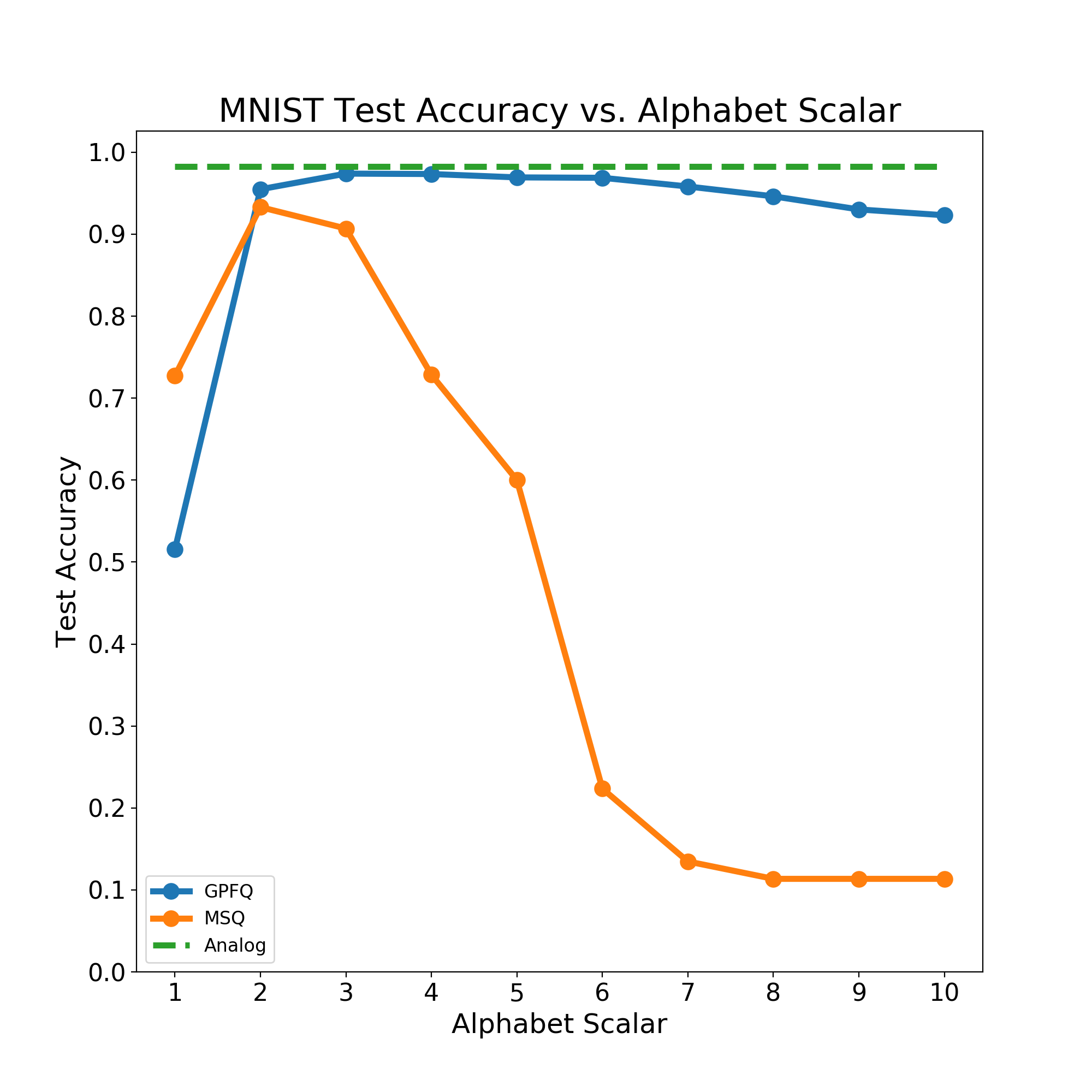
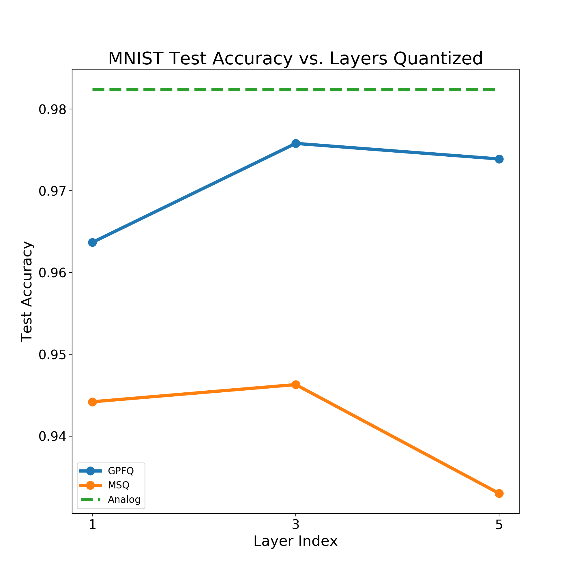
We trained a multilayer perceptron to classify MNIST digits ( images) with two hidden layers. The first layer has 500 neurons, the second has 300 neurons, and the output layer has 10 neurons. We also used batch normalization layers (Ioffe and Szegedy, 2015) after each hidden layer and chose the ReLU activation function for all layers except the last where we used softmax. We trained the unquantized network on the full training set of digits without any preprocessing. of the training data was used as validation during training. We then tested on the remaining images not used in the training set. We used categorical cross entropy as our loss function during training and the Adam optimizer—see Kingma and Ba (2014)—for 100 epochs with a minibatch size of 128. After training the unquantized model we used samples from the training set to train the quantization. We used the same data to quantize each layer rather than splitting the data for each layer. For this experiment we restricted the alphabet to be ternary and cross-validated over the alphabet scalar . The results for each choice of are displayed in Figure 1(a). As a benchmark we compared against a network quantized using MSQ, so each weight was quantized to the element of that is closest to it. As we see in Figure 1(a), the MSQ quantized network exhibits a high variability in its performance as a function of the alphabet scalar, whereas the GPFQ quantized network exhibits more stable behavior. Indeed, for a number of consecutive choices of the performance of the GPFQ quantized network was close to its unquantized counterpart. To illustrate how accuracy was affected as subsequent layers were quantized, we ran the following experiment. First, we chose the best alphabet scalar for each of the MSQ and GPFQ quantized networks separately. We then measured the test accuracy as each subsequent layer of the network was quantized, leaving the later ones unchanged. The median time it took to quantize a network was 288 seconds, or about 5 minutes. The results for MSQ and GPFQ are shown in Figure 1(b). Figure 1(b) demonstrates that GPFQ is able to “error correct” in the sense that quantizing a later layer can correct for errors introduced when quantizing previous ones. We also remark that in this setting we replace 32 bit floating point weights with bit weights. Consequentially, we have compressed the network by a factor of approximately , and yet the drop in test accuracy for GPFQ was minimal. Further, this quick calculation assumes we use bits to represent those weights which are quantized to zero. However, there are other important consequences for setting weights to zero. From a hardware perspective, the benefit is that forward propagation requires less energy due to there being fewer connections between layers. From a software perspective, multiplication by zero is an incredibly stable operation.
6.2 Convolutional Neural Network with CIFAR10
Even though our theory was phrased in the language of multilayer perceptrons it is easy to rephrase it using the vocabulary of convolutional neural networks. Here, neurons are kernels and the data are patches from the full images or their feature data in the hidden layers. These patches have the same dimensions as the kernel. Matrix convolution is defined in terms of Hilbert-Schmidt inner products between the kernel and these image patches. In other words, if we were to vectorize both the kernel and the image patches then we could take the usual inner product on vectors and reduce back to the case of a multilayer perceptron. This is exactly what we do in the quantization algorithm. Since every channel of the feature data has its own kernel we quantize each channel’s kernel independently.
We trained a convolutional neural network to classify images from the CIFAR10 data set with the following architecture
Here, C3 denotes two convolutional layers with kernels of size , MP2 denotes a max pooling layer with kernels of size , and denotes a fully connected layer with neurons. Not listed in the above schematic are batch normalization layers which we place before every convolutional and fully connected layer except the first. During training we also use dropout layers after the max pooling layers and before the final output layer. We use the ReLU function for every layer’s activation function except the last layer where we use softmax. We preprocess the data by dividing the pixel values by which normalizes them in the range . We augment the data set with width and height shifts as well as horizontal flips for each image. Finally, we train the network to minimize categorical cross entropy using stochastic gradient descent with a learning rate of , momentum of , and a minibatch size of 64 for 400 epochs. For more information on dropout layers and pooling layers see, for example, Hinton et al. (2012) and Weng et al. (1992), respectively.
We trained the unquantized network on the full set of training images. For training the quantization we only used the first images from the training set. As we did with the multilayer perceptron on MNIST, we cross-validated the alphabet scalars over the range and chose the best scalar for the benchmark MSQ network and the best GPFQ quantized network separately. Additionally, we cross-validated over the number of elements in the quantization alphabet, ranging over the set which corresponds to the set of bit budgets . The median time it took to quantize the network using GPFQ was 1830 seconds, or about 30 minutes. The results of these experiments are shown in Table 1. In particular, the table shows that the performance of GPFQ degrades gracefully as the bit budget decreases, while the performance of MSQ drops dramatically.
| CIFAR10 Top-1 Test Accuracy | ||||
| Bits | Analog | GPFQ | MSQ | |
| 2 | 0.8922 | 0.7487 | 0.1347 | |
| 3 | 0.8922 | 0.7350 | 0.1464 | |
| 4 | 0.8922 | 0.6919 | 0.0991 | |
| 5 | 0.8922 | 0.5627 | 0.1000 | |
| 6 | 0.8922 | 0.3515 | 0.1000 | |
| 2 | 0.8922 | 0.7522 | 0.2209 | |
| 3 | 0.8922 | 0.8036 | 0.2800 | |
| 2 | 4 | 0.8922 | 0.7489 | 0.1742 |
| 5 | 0.8922 | 0.6748 | 0.1835 | |
| 6 | 0.8922 | 0.5365 | 0.1390 | |
| 2 | 0.8922 | 0.7942 | 0.4173 | |
| 3 | 0.8922 | 0.8670 | 0.3754 | |
| 3 | 4 | 0.8922 | 0.8710 | 0.5014 |
| 5 | 0.8922 | 0.8567 | 0.5652 | |
| 6 | 0.8922 | 0.8600 | 0.5360 | |
| 2 | 0.8922 | 0.8124 | 0.4525 | |
| 3 | 0.8922 | 0.8778 | 0.7776 | |
| 4 | 4 | 0.8922 | 0.8879 | 0.8443 |
| 5 | 0.8922 | 0.8888 | 0.8291 | |
| 6 | 0.8922 | 0.8810 | 0.7831 | |
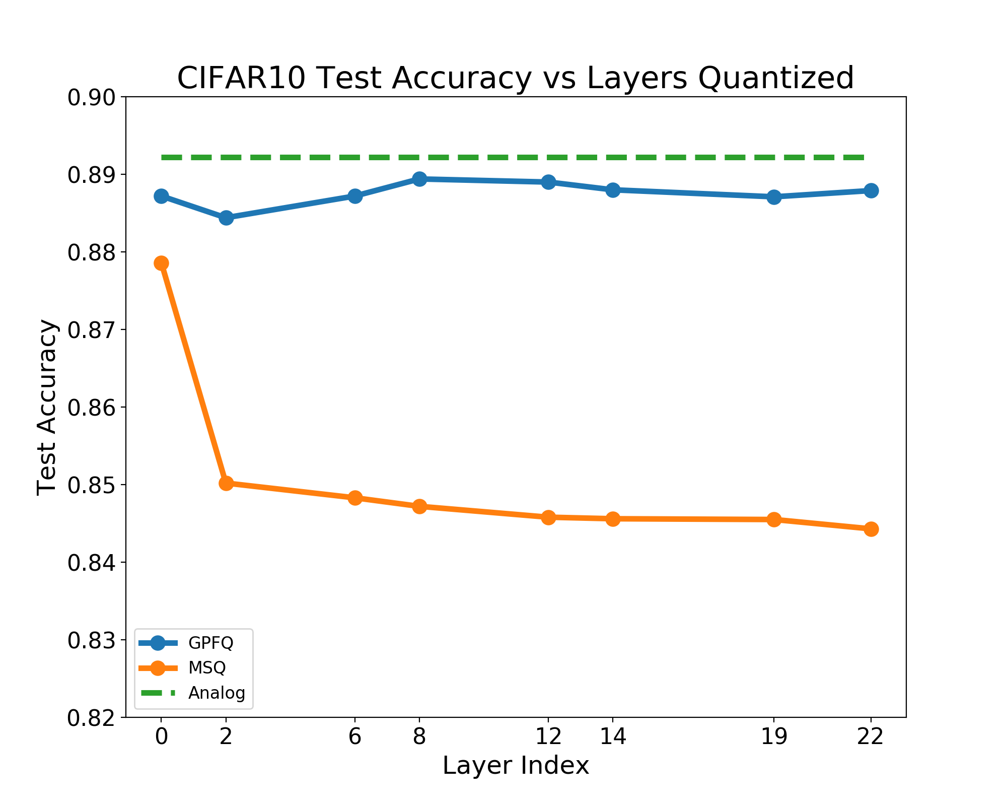
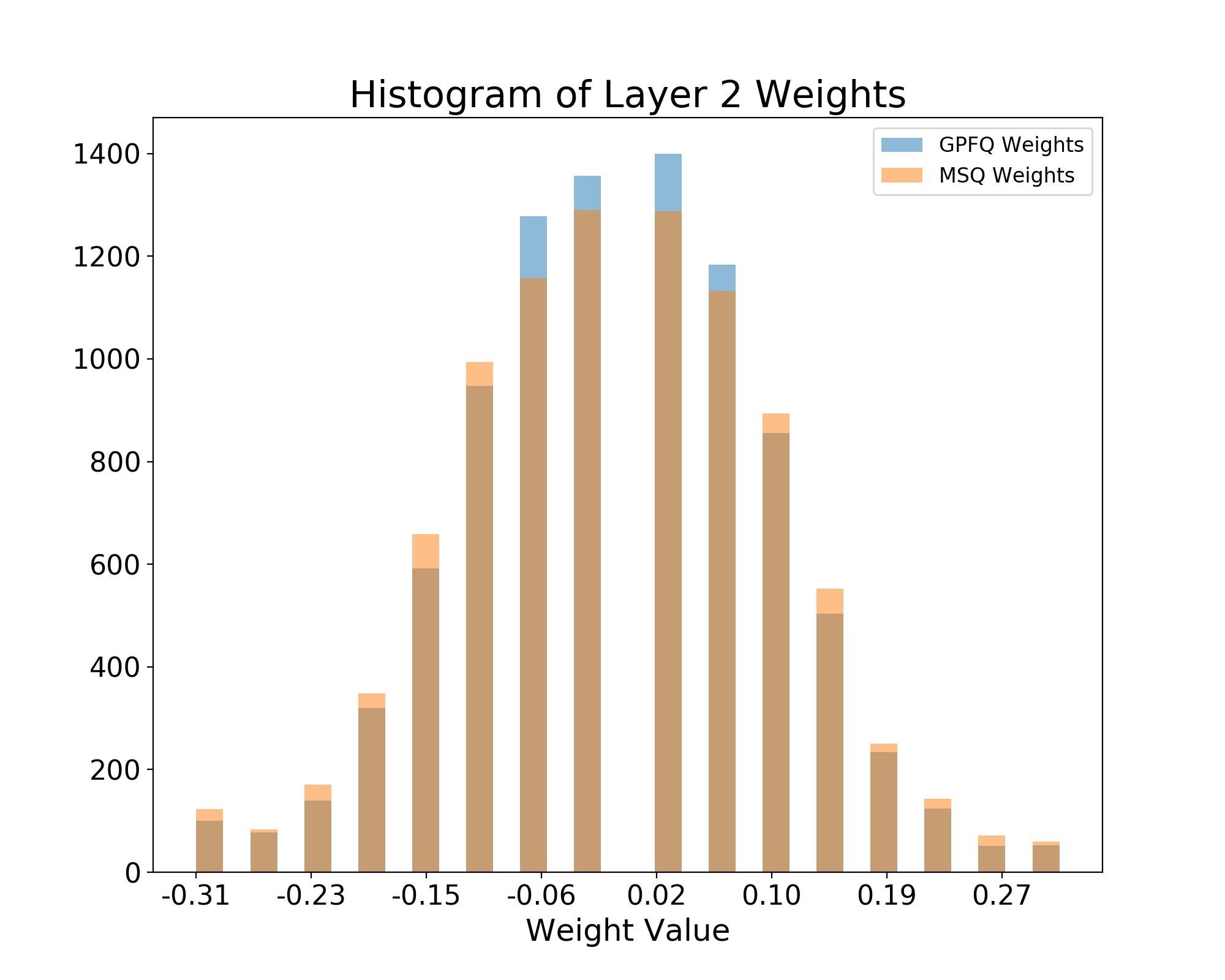
In this experiment, the best bit budget for both MSQ and GPFQ networks was bits, or characters in the alphabet. We plot the test accuracies for the best MSQ and the best GPFQ quantized network as each layer is quantized in Figure 2(a). Both networks suffer from a drop in test accuracy after quantizing the second layer, but (like in the first experiment) GPFQ recovers from this dip in subsequent layers while MSQ does not. Finally, to illustrate the difference between the two sets of quantized weights in this layer we histogram the weights in Figure 2(b).
6.3 VGG16 on Imagenet Data
The previous experiments were restricted to settings where there are only 10 categories of images. To illustrate that our quantization scheme and our theory work well on more complex data sets we considered quantizing the weights of VGG16 (Simonyan and Zisserman, 2014) for the purpose of classifying images from the ILSVRC2012 validation set (Russakovsky et al., 2015). This data set contains 50,000 images with 1,000 categories. Since 90% of all weights in VGG16 are in the fully connected layers, we took a similar route as Gong et al. (2014) and only considered quantizing the weights in the fully connected layers. We preprocessed the images in the manner that the ImageNet guidelines specify. First, we resize the smallest edge of the image to 256 pixels by using bicubic interpolation over pixel neighborhoods, and resizing the larger edge of the image to maintain the original image’s aspect ratio. Next, all pixels outside the central pixels are cropped out. The image is then saved with red, green, blue (RGB) channel order111We would like to thank Caleb Robinson for outlining this procedure in his GitHub repo found at https://github.com/calebrob6/imagenet_validation.. Finally, these processed images are further preprocessed by the function specified for VGG16 in the Keras preprocessing module. For this experiment we restrict the GPFQ quantizer to the alphabet . We cross-validate over the alphabet scalar . 1500 images were randomly chosen to learn the quantization. To assess the quality of the quantized network we used 20000 randomly chosen images disjoint from the set of images used to perform the quantization and measured the top-1 and top-5 accuracy for the original VGG16 model, GPFQ, and MSQ networks. The median time it took to quantize VGG16 using GPFQ was 15391 seconds, or about 5 hours. The results from this experiment can be found in Table 2. Remarkably, the best GPFQ network is able to get within and of the top-1 and top-5 accuracy of the analog model, respectively. In contrast, the best MSQ model can do is get within and of the top-1 and top-5 accuracy of the analog model, respectively. Importantly, as we saw in the previous two experiments, here again we observe a notable instability of test accuracy with respect to for the MSQ model whereas for the GPFQ model the test accuracy is more well-controlled. Moreover, just as in the CIFAR10 experiment, we see in these experiments that GPFQ networks uniformly outperform MSQ networks across quantization hyperparameter choices in both top-1 and top-5 test accuracy.
| ILSVRC2012 Test Accuracy | ||||||
|---|---|---|---|---|---|---|
| Analog Top-1 | Analog Top-5 | GPFQ Top-1 | GPFQ Top-5 | MSQ Top-1 | MSQ Top-5 | |
| 2 | 0.7073 | 0.8977 | 0.6901 | 0.8892 | 0.68755 | 0.88785 |
| 3 | 0.7073 | 0.8977 | 0.70075 | 0.8935 | 0.69485 | 0.8921 |
| 4 | 0.7073 | 0.8977 | 0.69295 | 0.89095 | 0.66795 | 0.8713 |
| 5 | 0.7073 | 0.8977 | 0.68335 | 0.88535 | 0.53855 | 0.77005 |
7 Future Work
Despite all of the analysis that has gone into proving stability of quantizing the first layer of a neural network using the dynamical system (4) and isotropic Gaussian data, there are still many interesting and unanswered questions about the performance of this quantization algorithm. The above experiments suggest that our theory can be generalized to account for non-Gaussian feature data which may have hidden dependencies between them. Beyond the subspace model we consider in Lemma 16, it would be interesting to extend the results to apply in the case of a manifold structure, or clustered feature data, whose intrinsic complexities can be used to improve the upper bounds in Theorem 2 and Theorem 3. Furthermore, it would be desirable to extend the analysis to address quantizing all of the hidden layers. As we showed in the experiments, our set-up naturally extends to the case of quantizing convolutional layers. Another extension of this work might consider modifying our quantization algorithm to account for other network models like recurrent networks. Finally, we observed in Theorem 2 that the relative training error for learning the quantization decays like . We also observed in the discussion at the end of Section 4 that when all of the feature data were the same our quantization algorithm reduced to a first order greedy quantizer. Higher order quantizers in the context of oversampled finite frame coefficients and bandlimited functions are known to have quantization error which decays polynomially in terms of the oversampling rate. One wonders if there exist extensions of our algorithm, perhaps with a modest increase in computational complexity, that achieve faster rates of decay for the relative quantization error. We leave all of these questions for future work.
8 Proofs: Supporting Lemmata
This section presents supporting lemmata that characterize the geometry of the dynamical system (4), as well as standard results from high dimensional probability which we will use in the proof of the main technical result, Theorem 14, which appears in Section 9. Outside of the high dimensional probability results, the results of Lemmas 9, 11 and 12 consider the behavior of the dynamical system under arbitrarily distributed data.
Lemma 7
Vershynin (2018) Let . Then for any
Lemma 8
Vershynin (2018) Let be an -dimensional standard Gaussian vector. Then there exists some universal constant so that for any
Lemma 9
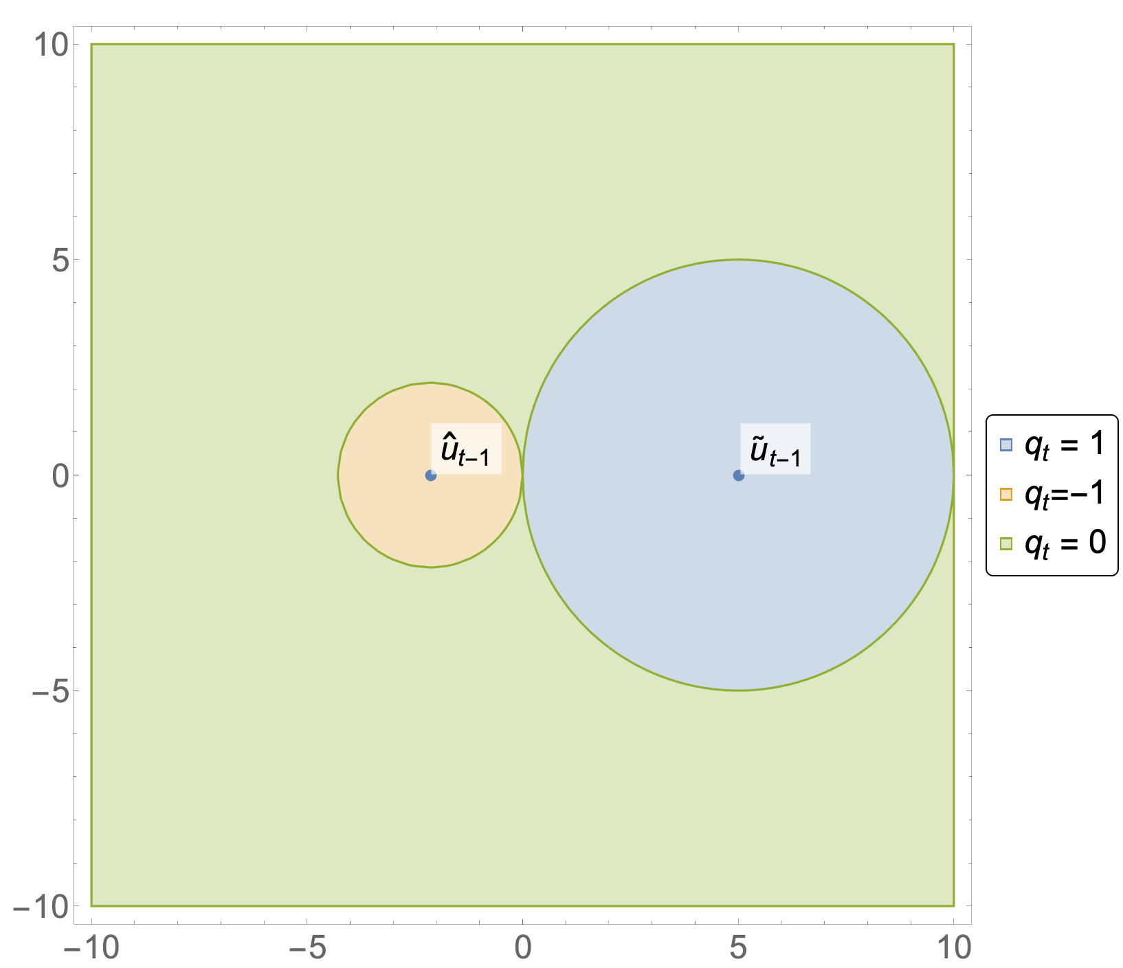
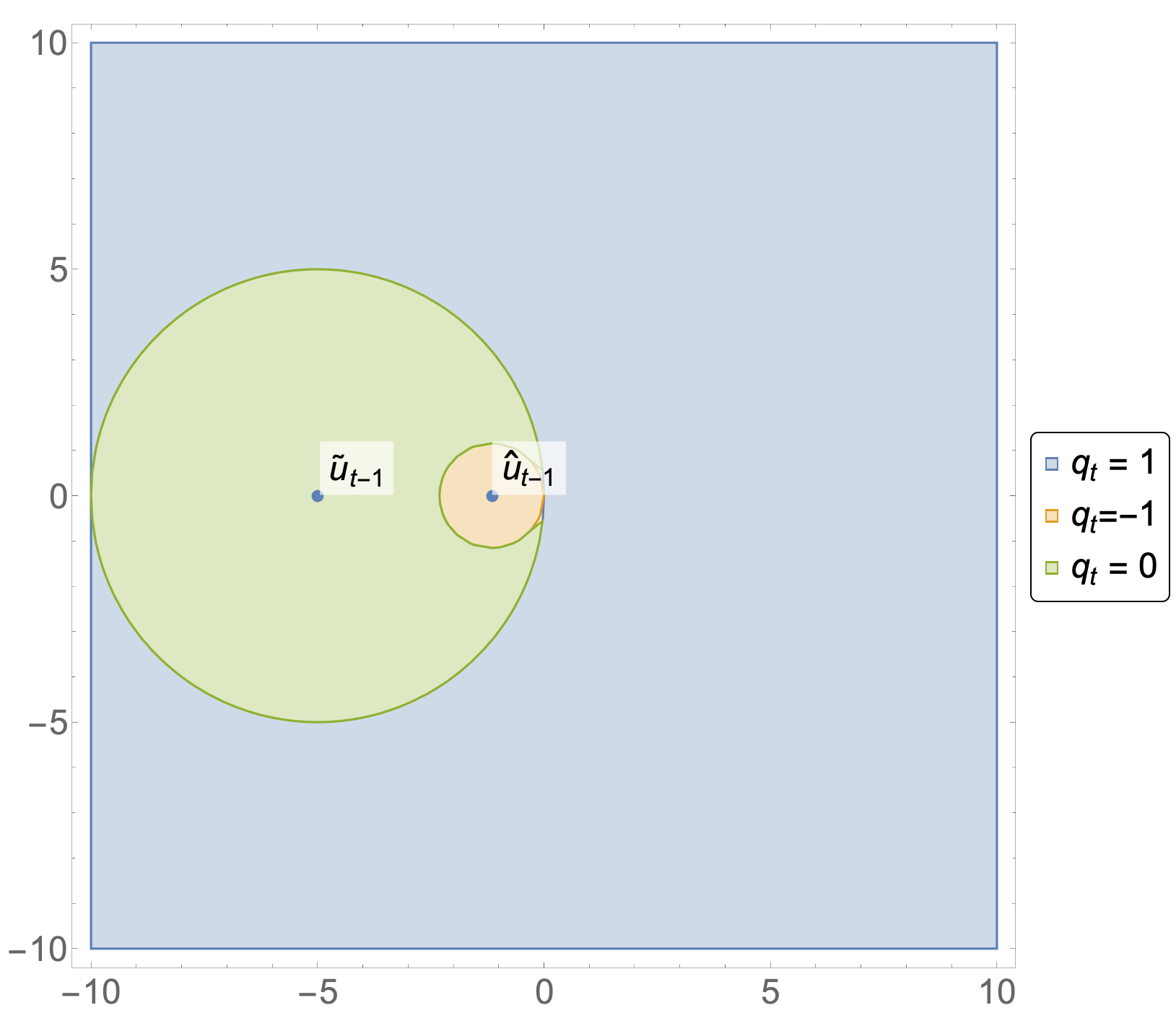
Suppose that . Then
Proof When , (4) implies that
| (11) |
Since , . After dividing both sides of (11) by this factor, and recalling that , we may complete the square to get the equivalent inequality
An analogous argument shows the claim for the level set .
Remark 10
When or , the algebra in the proof tells us that the set of for (resp. ) is actually the complement of , (resp. the complement of ). For the special case when these level sets are half-spaces.
Lemma 11
Suppose , and a random vector in . Then
where is the probability measure over induced by the random variable .
Proof Let denote the event that for . Then by the law of total probability
Therefore, we need to look at each summand in the above sum. Well, precisely when . So we have
Next, precisely when . Noting that , we have
Finally, precisely when . So we have
Summing these three piecewise functions yields the result.
Lemma 12
When , we have
Corollary 13
If with probability , then with probability 1.
9 Proofs: Core Lemmata
We start by proving our main result, Theorem 14, and its extension to the case where feature vectors live in a low-dimensional subspace, Lemma 16. The proof of Theorem 14 relies on bounding the moment generating function of , which in turn requires a number of results, referenced in the proof and presented thereafter. These lemmas carefully deal with bounding the above moment generating function on the events where is fixed. Given and , Lemma 9 tells us the set of directions which result in and these are the relevant events one needs to consider when bounding the moment generating function. Lemma 17 handles the case when , Lemma 18 handles the case when , and Lemma 19 handles the case when .
Theorem 14
Suppose that for , the vectors are independent and that are i.i.d. and independent of , and define the event
Then there exist positive constants , , and , such that with , and satisfying , the iteration (4) satisfies
| (12) |
Above, is a universal constant and .
Proof The proof technique is inspired by Hajek (1982). Define the events
Using a union bound and Lemma 8, we see that happens with low probability since
We can therefore bound the probability of interest with appropriate conditioning.
Looking at the first summand, for any , we have by Markov’s inequality
We expand the conditional expectation given the filtration into a sum of two parts
Towering expectations, the expectation over of the first summand is bounded above by for all on the event using Lemmas 17, 18, and 19. Therefore, the same bound is also true for the expectation over . As for the second term, we have
For both terms, we can use the uniform bound on the increments as proven in Corollary 13. The first term we can bound by . As for the second, expecting over the draw of gives us
Therefore, we have
Proceeding inductively on yields the claim.
Remark 15
Lemma 16
Suppose where satisfies , and has i.i.d. entries. In other words, suppose the feature data are Gaussians drawn from a -dimensional subspace of . Then with the remaining hypotheses as Theorem 14 we have with probability at least
Proof We will show that running the dynamical system (4) with is equivalent to running a modified version of (4) with the columns of , denoted . Then we can apply the result of Theorem 14. By definition, we have
In anticipation of subsequent applications of change of variables, let be the singular value decomposition of where and are orthogonal matrices and decomposes as
Since is a linear combination of for all it follows that is in the column space of . In other words, . We may rewrite the above dynamical system in terms of as
So, in other words, we’ve reduced to running (4) but now with the state variables in place of and with in place of . Applying the result of Theorem 14 yields the claim.
Lemma 17
Let and . Define the event
and set , where is some constant and is as in Lemma 8. Then there exists a universal constant so that with
Proof

Recall . Let us first consider the case when . We will further assume that , since there is the symmetry between and under the mapping . Before embarking on our calculus journey, let us make some key remarks. First, on the event , we can bound the increment above by . So, it behooves us to find an upper bound for . Since the exponential function is non-negative, we can always upper bound this expectation by removing the indicator on . In other words,
| (13) |
Since we’re indicating on an event where , we will need to handle the events where with some care, since without an a priori upper bound on the moment generating function restricted to this event could explode. Therefore, we’ll divide the region of integration into 4 pieces which are depicted in Figure 4. Because of the abundance of notation in the following arguments, we will denote .
Let’s handle the easier event first, namely where . Here, we have
| (14) |
By rotational invariance, we may assume without loss of generality that , where is the first standard basis vector. In that case, the constraint is equivalent to , where is the first component of . Using Lemma 9, it follows that the set of for which and is simply , where the negative sign here comes from the fact that . That means we can rewrite (9) as
Perhaps surprisingly, we can afford to use the crude upper bound on this integral by simply removing the constraint that . Iterating the univariate integrals then gives us
| (15) |
We complete the square and use a change of variables to reformulate (9) as
| (16) |
Since the lower limit of integration is positive and large when is, we can use a tail bound as in Lemma 7 to upper bound (9) by
| (17) |
where the first inequality follows from and the equality follows from
.
Now we handle the moment generating function on the event that . Again, using rotational invariance to assume , we have by Lemma 9 that the event to integrate over is . Notice that iterating the integrals gives us
| (18) |
with the notation for . Consequentially, we can rephrase (9) into a more probabilistic statement. Below, let denote i.i.d. standard normal random variables. Then (9) is equal to
| (19) |
The probability appearing in (19) will decay exponentially provided is sufficiently large. To that end, we will divide up this half-space into the following regions. Let be a constant and define the sets , , and . Figure 4 gives a visual depiction of this decomposition. Then we have
For the integral over , we will use the naïve upper bound
This gives us
| (20) |
The upper limit of integration is negative since . Under this assumption, we can upper bound the integral with a Riemann sum. As the maximum of the integrand occurs at the upper limit of integration, we bound (9) with
| (21) |
Recognizing that and recalling that we can further upper bound by
| (22) |
As was the case for , we can use the bound over too. Completing the square in the exponent as we usually do gives us
| (23) |
Since the lower limit of integration is positive, so we can use a Gaussian tail bound as in Lemma 7 to bound (9) by
| (24) |
As the exponent appearing in (9) is negative. Bounding the exponential by then gives us the upper bound
| (25) |
Now, for we can use the exponential decay of the probability appearing in (19). To make the algebra a bit nicer, we can upper-bound this probability by since on we have . Setting , Lemma 8 tells us for
To simplify our algebra, we remark that for any ,
provided . By our choice of , this happens to be the case on , as and so
This gives us the upper bound on the probability
Consequentially, we can bound the integral over as follows
| (26) |
Setting , we have that (9) is equal to
| (27) |
We remark that if which holds since . Therefore, the lower limit of integration is positive and we can use a Gaussian tail bound as in Lemma 7 to upper bound (9) by
| (28) | ||||
| (29) |
Putting it all together, and remembering to add back in the factor we have previously ignored, we’ve bound from above with
So, when and the claim follows.
Now, let’s consider the case when . Then it must be, by Lemma 9, that . By non-negativity of the exponential function, we can always upper-bound the moment generating function by instead integrating over . Pictorially, one can see this by looking at the subfigure on the right in Figure 3. In this scenario, we’re integrating over the region in green. The upper bound we’re proposing is derived by ignoring the constraint from the blue region on the left half-space. Using this upper bound we can retrace through the steps we took to bound the integrals over and with only minor modifications and obtain the desired result. By symmetry, an analogous approach will work for .
Lemma 18
With the same hypotheses as Lemma 17,
Proof To begin, let’s consider the case when . Recalling that , and arguing as we did at the beginning of the proof of Lemma 17, Lemma 9 tells us
As before, we have denoted for conciseness. Using rotational invariance, we may assume that . Just as we did in Lemma 17, expressing this integral as nested iterated integrals gives us the probabilistic formulation
where, as before, the are i.i.d. standard normal random variables. So, consider decomposing the above integral into the following two pieces. Set and where is a fixed constant. Then on we have by Lemma 8
Setting aside the factor for the moment, we have that the integral over is equal to
| (30) |
We remark that the lower limit of integration is strictly positive. Therefore, using a Riemann approximation to the integral and knowing that the maximum of the integral occurs at the lower limit of integration bounds (9) above by
| (31) |
On , we use the bound to get
| (32) | ||||
| (33) |
Since the lower limit of integration is strictly positive, we can use a Gaussian tail bound as in Lemma 7 to upper bound (32) by
| (34) |
To summarize, we have shown, at least when , that
| (35) |
Therefore, when , (9) is bounded above by as desired.
Now, let’s consider the case when . In this scenario, we can express the expectation as
Using the exact same approach as in the proof of Lemma 17, we can partition the domain of integration into the following pieces:
The same arguments from the proof of Lemma 17 apply here with only minor modifications. Namely, an argument exactly like that given for (9) gives us
Similarly, the chain of logic used to derive (9) gives us
Calculations for the derivation of (28) give us
Finally, the same reasoning that was used to derive (22) gives us
Following the remainder of the proof of Lemma 17 in this scenario gives us the result when .
Lemma 19
With the same hypotheses as Lemma 17
Proof
The proof is effectively the same as that for Lemma 18.
Acknowledgments
This work was supported in part by National Science Foundation Grant DMS-2012546 and a UCSD senate research award.
References
- Ajtai (1998) Miklos Ajtai. The shortest vector problem in l2 is np-hard for randomized reductions. In Proceedings of the thirtieth annual ACM symposium on Theory of computing, pages 10–19, 1998.
- Baldi and Vershynin (2019) Pierre Baldi and Roman Vershynin. The capacity of feedforward neural networks. Neural networks, 116:288–311, 2019.
- Banaszczyk (1990) Wojciech Banaszczyk. A beck—fiala-type theorem for euclidean norms. European Journal of Combinatorics, 11(6):497–500, 1990.
- Banaszczyk (1998) Wojciech Banaszczyk. Balancing vectors and gaussian measures of n-dimensional convex bodies. Random Structures & Algorithms, 12(4):351–360, 1998.
- Bansal (2010) Nikhil Bansal. Constructive algorithms for discrepancy minimization. In 2010 IEEE 51st Annual Symposium on Foundations of Computer Science, pages 3–10. IEEE, 2010.
- Bansal et al. (2018) Nikhil Bansal, Daniel Dadush, Shashwat Garg, and Shachar Lovett. The gram-schmidt walk: a cure for the banaszczyk blues. In Proceedings of the 50th Annual ACM SIGACT Symposium on Theory of Computing, pages 587–597, 2018.
- Chollet et al. (2015) François Chollet et al. Keras. https://keras.io, 2015.
- Courbariaux et al. (2015) Matthieu Courbariaux, Yoshua Bengio, and Jean-Pierre David. Binaryconnect: Training deep neural networks with binary weights during propagations. In Advances in neural information processing systems, pages 3123–3131, 2015.
- Cybenko (1989) George Cybenko. Approximation by superpositions of a sigmoidal function. Mathematics of control, signals and systems, 2(4):303–314, 1989.
- Dadush et al. (2016) Daniel Dadush, Shashwat Garg, Shachar Lovett, and Aleksandar Nikolov. Towards a constructive version of banaszczyk’s vector balancing theorem. arXiv preprint arXiv:1612.04304, 2016.
- Daubechies and DeVore (2003) Ingrid Daubechies and Ron DeVore. Approximating a bandlimited function using very coarsely quantized data: A family of stable sigma-delta modulators of arbitrary order. Annals of mathematics, 158(2):679–710, 2003.
- Eldan and Singh (2014) Ronen Eldan and Mohit Singh. Efficient algorithms for discrepancy minimization in convex sets. arXiv preprint arXiv:1409.2913, 2014.
- Giannopoulos (1997) Apostolos A Giannopoulos. On some vector balancing problems. Studia Mathematica, 122(3):225–234, 1997.
- Gong et al. (2014) Yunchao Gong, Liu Liu, Ming Yang, and Lubomir Bourdev. Compressing deep convolutional networks using vector quantization. arXiv preprint arXiv:1412.6115, 2014.
- Goodfellow et al. (2016) Ian Goodfellow, Yoshua Bengio, Aaron Courville, and Yoshua Bengio. Deep learning, volume 1. MIT press Cambridge, 2016.
- Guo (2018) Yunhui Guo. A survey on methods and theories of quantized neural networks. arXiv preprint arXiv:1808.04752, 2018.
- Gupta et al. (2015) Suyog Gupta, Ankur Agrawal, Kailash Gopalakrishnan, and Pritish Narayanan. Deep learning with limited numerical precision. In International Conference on Machine Learning, pages 1737–1746, 2015.
- Hajek (1982) Bruce Hajek. Hitting-time and occupation-time bounds implied by drift analysis with applications. Advances in Applied probability, pages 502–525, 1982.
- Han et al. (2016) Song Han, Huizi Mao, and William J Dally. Deep compression: Compressing deep neural networks with pruning, trained quantization and huffman coding. arXiv preprint arXiv:1510.00149, conference paper at ICLR, 2016.
- Harvey et al. (2014) Nicholas JA Harvey, Roy Schwartz, and Mohit Singh. Discrepancy without partial colorings. In Approximation, Randomization, and Combinatorial Optimization. Algorithms and Techniques (APPROX/RANDOM 2014). Schloss Dagstuhl-Leibniz-Zentrum fuer Informatik, 2014.
- Hinton et al. (2012) Geoffrey E Hinton, Nitish Srivastava, Alex Krizhevsky, Ilya Sutskever, and Ruslan R Salakhutdinov. Improving neural networks by preventing co-adaptation of feature detectors. arXiv preprint arXiv:1207.0580, 2012.
- Hubara et al. (2017) Itay Hubara, Matthieu Courbariaux, Daniel Soudry, Ran El-Yaniv, and Yoshua Bengio. Quantized neural networks: Training neural networks with low precision weights and activations. The Journal of Machine Learning Research, 18(1):6869–6898, 2017.
- Inose et al. (1962) Hi Inose, Y Yasuda, and Jun Murakami. A telemetering system by code modulation--modulation. IRE Transactions on Space Electronics and Telemetry, (3):204–209, 1962.
- Ioffe and Szegedy (2015) Sergey Ioffe and Christian Szegedy. Batch normalization: Accelerating deep network training by reducing internal covariate shift. arXiv preprint arXiv:1502.03167, 2015.
- Kim et al. (2016) Yong-Deok Kim, Eunhyeok Park, Sungjoo Yoo, Taelim Choi, Lu Yang, and Dongjun Shin. Compression of deep convolutional neural networks for fast and low power mobile applications. arXiv preprint arXiv:1511.06530, conference paper at ICLR, 2016.
- Kingma and Ba (2014) Diederik P Kingma and Jimmy Ba. Adam: A method for stochastic optimization. arXiv preprint arXiv:1412.6980, 2014.
- Kolda and O’leary (1998) Tamara G Kolda and Dianne P O’leary. A semidiscrete matrix decomposition for latent semantic indexing information retrieval. ACM Transactions on Information Systems (TOIS), 16(4):322–346, 1998.
- Kueng and Tropp (2019) Richard Kueng and Joel A Tropp. Binary component decomposition part ii: The asymmetric case. arXiv preprint arXiv:1907.13602, 2019.
- LeCun et al. (2015) Yann LeCun, Yoshua Bengio, and Geoffrey Hinton. Deep learning. nature, 521(7553):436, 2015.
- Lovasz et al. (1986) Laszlo Lovasz, Joel Spencer, and Katalin Vesztergombi. Discrepancy of set-systems and matrices. European Journal of Combinatorics, 7(2):151–160, 1986.
- Lovett and Meka (2015) Shachar Lovett and Raghu Meka. Constructive discrepancy minimization by walking on the edges. SIAM Journal on Computing, 44(5):1573–1582, 2015.
- Menshikov et al. (2016) Mikhail Menshikov, Serguei Popov, and Andrew Wade. Non-homogeneous random walks: Lyapunov function methods for near-critical stochastic systems, volume 209. Cambridge University Press, 2016.
- Meyn and Tweedie (2012) Sean P Meyn and Richard L Tweedie. Markov chains and stochastic stability. Springer Science & Business Media, 2012.
- Pemantle and Rosenthal (1999) Robin Pemantle and Jeffrey S Rosenthal. Moment conditions for a sequence with negative drift to be uniformly bounded in lr. Stochastic Processes and their Applications, 82(1):143–155, 1999.
- Rastegari et al. (2016) Mohammad Rastegari, Vicente Ordonez, Joseph Redmon, and Ali Farhadi. Xnor-net: Imagenet classification using binary convolutional neural networks. In European conference on computer vision, pages 525–542. Springer, 2016.
- Rothvoss (2017) Thomas Rothvoss. Constructive discrepancy minimization for convex sets. SIAM Journal on Computing, 46(1):224–234, 2017.
- Russakovsky et al. (2015) Olga Russakovsky, Jia Deng, Hao Su, Jonathan Krause, Sanjeev Satheesh, Sean Ma, Zhiheng Huang, Andrej Karpathy, Aditya Khosla, Michael Bernstein, Alexander C. Berg, and Li Fei-Fei. ImageNet Large Scale Visual Recognition Challenge. International Journal of Computer Vision (IJCV), 115(3):211–252, 2015. doi: 10.1007/s11263-015-0816-y.
- Schmidhuber (2015) Jurgen Schmidhuber. Deep learning in neural networks: An overview. Neural networks, 61:85–117, 2015.
- Silver et al. (2016) David Silver, Aja Huang, Chris J Maddison, Arthur Guez, Laurent Sifre, George Van Den Driessche, Julian Schrittwieser, Ioannis Antonoglou, Veda Panneershelvam, Marc Lanctot, Sander Dieleman, Dominik Grewe, John Nham, Nal Kalchbrenner, Ilya Sutskever, Timothy Lillicrap, Madeleine Leach, Koray Kavukcuoglu, Thore Graepel, and Demis Hassabis. Mastering the game of go with deep neural networks and tree search. nature, 529(7587):484, 2016.
- Simonyan and Zisserman (2014) Karen Simonyan and Andrew Zisserman. Very deep convolutional networks for large-scale image recognition. arXiv preprint arXiv:1409.1556, 2014.
- Spencer (1985) Joel Spencer. Six standard deviations suffice. Transactions of the American mathematical society, 289(2):679–706, 1985.
- Vershynin (2018) Roman Vershynin. High-dimensional probability: An introduction with applications in data science, volume 47. Cambridge university press, 2018.
- Wang and Cheng (2017) Peisong Wang and Jian Cheng. Fixed-point factorized networks. In Proceedings of the IEEE Conference on Computer Vision and Pattern Recognition, pages 4012–4020, 2017.
- Weng et al. (1992) Juyang Weng, Narendra Ahuja, and Thomas S Huang. Cresceptron: a self-organizing neural network which grows adaptively. In [Proceedings 1992] IJCNN International Joint Conference on Neural Networks, volume 1, pages 576–581. IEEE, 1992.