All block maxima method for estimating the extreme value index

Abstract

The block maxima (BM) approach in extreme value analysis fits a sample of block maxima to the Generalized Extreme Value (GEV) distribution. We consider all potential blocks from a sample, which leads to the All Block Maxima (ABM) estimator. Different from existing estimators based on the BM approach, the ABM estimator is permutation invariant. We show the asymptotic behavior of the ABM estimator, which has the lowest asymptotic variance among all estimators using the BM approach. Simulation studies justify our asymptotic theories. A key step in establishing the asymptotic theory for the ABM estimator is to obtain asymptotic expansions for the tail empirical process based on higher order statistics with weights.

Keywords: Block maxima method; maximum likelihood estimation; weighted tail empirical process; Radon-Nikodym derivative; heavy-tails

MSC 2020 subject classifications: 62G32; 62G30

1 Introduction

Consider a random sample $\{X_{1},X_{2},...,X_{n}\}$ with a common distribution function $F$ and assume that $F$ belongs to the domain of attraction of a Generalized Extreme Value (GEV) distribution: there exist some sequences $a_{n}>0$ and $b_{n}$ such that

$$\lim_{n\to\infty}F^{n}(a_{n}x+b_{n})=G_{\gamma}(x)=\exp(-(1+x\gamma)^{-1/\gamma}),\text{ for }1+\gamma x>0.$$ (1.1)

The only parameter $\gamma$ in the limit distribution is called the extreme value index. It governs not only the limit distribution but also the tail behavior of the original distribution $F$.

To estimate $\gamma$, the classical Block Maxima (BM) approach follows from the domain of attraction condition. One may divide the entire sample into $k$ disjoint blocks of size $m=n/k$ and fit the corresponding block maxima to the GEV distribution, for example, by the Maximum Likelihood (ML) method. This results in an estimator of $(\gamma,a_{m},b_{m})$. Such estimators are consistent and jointly asymptotically normal under mild conditions (Bücher and Segers, 2017; Dombry and Ferreira, 2019). Besides constructing blocks disjointly, one may also construct blocks in various ways to increase the number of block maxima. For example, Bücher and Segers (2018a) construct a sliding block estimator that is more efficient by considering the maxima of consecutive overlapping blocks, thereby introducing dependence between the block maxima even if the underlying observations are independent.

An undesired feature of all existing estimators from the BM approach is that they are not permutation invariant. If the observations are i.i.d., estimators of the parameter $\gamma$ should not depend on the order of the observations. However, for all existing BM estimators, based on either disjoint or sliding blocks, permutating the observations will in general not lead to the same estimate of $\gamma$. Based on this fact, Mefleh et al. (2019) construct a permutation bootstrap method for reducing the estimation uncertainty in estimators from the BM approach.

We propose to construct a permutation-invariant estimator, derived from a BM approach. Specifically, we consider all possible blocks of a fixed size $m$ that could have occured when sampling from the original observations. Denote $X_{1:n}\leq X_{2:n}\leq...\leq X_{n:n}$ as the order statistics of the random sample. The lowest observation that can be a block maximum is $X_{m:n}$. Note that $X_{m:n}$ can be the block maximum in one block only, that is, when the lowest $m$ observations form the block. In general, $X_{n-i+1:n}$ is a block maxima in $\binom{n-i}{m-1}$ blocks for $i=1,2,...,n-m+1$. Therefore, the multiset consisting of all block maxima

$$\left\{\underbrace{X_{n:n},...,X_{n:n}}_{\binom{n-1}{m-1}},...\underbrace{X_{n-i+1:n},...,X_{n-i+1:n}}_{\binom{n-i}{m-1}},...,\underbrace{X_{m:n}}_{1}\right\}$$

can be viewed as a repeated sample of order statistics, where $X_{n-i+1:n}$ is repeated $\binom{n-i}{m-1}$ times for $1\leq i\leq n-m+1$. Consequently, the multiset contains $\binom{n}{m}$ repeated observations. We fit this multiset of all block maxima to the GEV distribution by means of the ML method as if they are i.i.d. observations. This results in a permutation-invariant estimator of $(\gamma,a_{m},b_{m})$ — the All Block Maxima (ABM) estimator. Note that the idea of considering statistics based on all blocks has been investigated in Segers (2001, Chapter 5). Nevertheless, only consistency has been studied therein, whereas we aim at establishing the asymptotic normality of the ABM estimator.

A heuristic rationale for the validity of the ABM estimator can be provided by considering an equivalent characterization of $F$ belonging to the domain of attraction of a GEV distribution: the limit relation (1.1) is equivalent to the existence of a positive function $f$ such that

$$\lim_{t\uparrow x^{*}}\frac{1-F(t+xf(t))}{1-F(t)}=D_{\gamma}(x):=(1+\gamma x)^{-1/\gamma},\text{ for }1+\gamma x>0.$$ (1.2)

where $x^{*}=\sup\{x:F(x)<1\}$ and $1-D_{\gamma}(x)$ is the CDF of the Generalized Pareto (GP) distribution (de Haan and Ferreira, 2006, Theorem 1.1.6). Consequently, order statistics above a high threshold can be approximately regarded as order statistics from a GP distribution. One can assign proper weights to these order statistics in line with the Radon-Nikodym (RN) derivative between the GEV and GP distribution so that the resulting weighted order statistics will approximately follow a GEV distribution. In Section 2.2 we show that the repetition scheme of the order statistics present in the multiset of all block maxima corresponds to the RN derivative between the GEV and GP distribution. Therefore, fitting the sample of all block maxima to the GEV distribution by ML is a valid estimation method.

Our main theorem, Theorem 3.5, states the asymptotic normality of the ABM estimator when the observations are i.i.d. and $\gamma>0$. The proof relies heavily on a weighted tail empirical process result of the order statistics, presented in Proposition 3.6. This result is of independent interest and can be used for proving asymptotic behaviour of other estimators based on all block maxima.

The ABM estimator has a lower asymptotical variance than any other existing estimator using the BM approach. This theoretical result is confirmed by extensive simulation studies. Moreover, the simulation study further suggests that the ABM estimates against the effective number of observations used in estimation, $n/m$, yield a smooth path which facilitates a straightforward choice of the optimal number of blocks. Finally, the ABM estimator also perform better than the disjoint BM estimator when the observations are not i.i.d.: both for observations forming a serially dependent but stationary time series, and for observations drawn from non-stationary distributions.

2 The All Block Maxima Method: $\gamma>0$

We study and apply the ABM estimator in case of a positive extreme value index. For $\gamma>0$, the domain of attraction condition implies that for $\sigma_{n}=F^{\leftarrow}(1-1/n)$ and any $x>0$,

$$\lim_{n\to\infty}F^{n}(\sigma_{n}x)=\exp\left(-x^{-1/\gamma}\right).$$ (2.1)

Compared to the general domain of attraction condition in (1.1), the shift $b_{n}$ is set to zero and the normalizing constant $a_{n}$ is related to $\sigma_{n}$ by $\sigma_{n}=\gamma a_{n}$. Consequently, we can fit the sample of all block maxima $\ \underbrace{X_{n:n},...,X_{n:n}}_{\binom{n-1}{m-1}},...\underbrace{X_{n-i+1:n},...,X_{n-i+1:n}}_{\binom{n-i}{m-1}},...,\underbrace{X_{m:n}}_{1}$ to a scaled Fréchet distribution to estimate $(\gamma,\sigma_{n})$.

2.1 Weighted Maximum Likelihood for estimating $\gamma$

Similar to Bücher and Segers (2018b), we deal with potentially negative observations by left-truncating all the observations with a constant $c>0$. Denote $X_{i}^{c}=\max(X_{i},c)$ and denote the CDF of the scaled Fréchet distribution by $G(x;\theta)=\exp\left(-\left(\frac{x}{\sigma}\right)^{-1/\gamma}\right)$ for $x>0$, with shape and scale parameters $\theta=(\gamma,\sigma)\in(0,\infty)^{2}$. Note that in the context of ML estimation, the log-likelihood based on a sample of repeated observations can be viewed as a weighted log-likelihood for non-repeated observations. When fitting the sample of all block maxima to the scaled Fréchet distribution, the weight corresponding to the order statistic $X_{n-i+1:n}$ is

$$p_{i}=\binom{n-i}{m-1}/\binom{n}{m},\text{ with }\sum_{i=1}^{n-m+1}p_{i}=1.$$ (2.2)

The log-likelihood function is then

$$L(\theta) =\sum_{i=1}^{n-m+1}p_{i}l_{\theta}\left(X^{c}_{n-i+1:n}\right),$$ (2.3)

$$\mbox{ with }l_{\theta}(x) =\log\left(\frac{1}{\gamma\sigma}\right)-\left(\frac{x}{\sigma}\right)^{-1/\gamma}-(1/\gamma+1)\log\left(\frac{x}{\sigma}\right).$$ (2.4)

By taking the partial derivatives of $L(\theta)$ with respect to $\theta=(\gamma,\sigma)$, we obtain that the ML estimator $\hat{\gamma}$ is given by the zero of the function

$$\Psi_{n}(\gamma)=\gamma+\frac{\sum_{i=1}^{n-m+1}p_{i}\left(X^{c}_{n-i+1:n}\right)^{-1/\gamma}\log\left(X^{c}_{n-i+1:n}\right)}{\sum_{i=1}^{n-m+1}p_{i}\left(X^{c}_{n-i+1:n}\right)^{-1/\gamma}}-\sum_{i=1}^{n-m+1}p_{i}\log\left(X^{c}_{n-i+1:n}\right),$$

and the ML estimator for $\sigma$ is given by

$$\hat{\sigma}=\sum_{i=1}^{n-m+1}\left(p_{i}\left(X^{c}_{n-i+1:n}\right)^{-1/\hat{\gamma}}\right)^{-\hat{\gamma}}.$$

The existence and uniqueness of the ML estimator is guaranteed if the order statistics do not all have the same value. This follows directly from Lemma 2.1 in Bücher and Segers (2018b).

Finally, for practical purposes, instead of computing the binomial coefficients for each weight, it is more efficient to calculate the weights $p_{i}$ via the following recursion, initiated by $p_{1}=m/n$,

$$p_{i+1}=\left(\frac{n-m-i}{n-1-i}\right)p_{i},\hskip 28.45274pt\text{ for }1\leq i\leq n-m+1.$$

2.2 Measure Transformation

The ABM estimator can be heuristically understood by considering the measure transformation from a GP distribution to a GEV distribution. Here we present that heuristic argument in more detail for $\gamma>0$.

First, for $\gamma>0$, the measure transformation can be simplified to that from a Pareto to a Fréchet distribution because the domain of attraction condition (2.1) is equivalent to

$$\lim_{t\to\infty}\frac{1-F(tx)}{1-F(t)}:=H_{\gamma}(x)=x^{-1/\gamma}\text{ for all }x>0.$$ (2.5)

where $1-H_{\gamma}(x)$ is the CDF of a Pareto distribution with shape parameter $\gamma$. Effectively, for a large threshold $t$, excess ratios over the threshold follow a Pareto distribution. For example, take $t=X_{n-k:n}$, and denote $Y_{k-i+1:k}=X_{n-i+1:n}/t$ for $i=1,2,\ldots,k$, then $Y_{1:k}\leq\ldots\leq Y_{k:k}$ can be approximately viewed as order statistics from the Pareto distribution. Heuristically, we have $H_{\gamma}(Y_{k-i+1:k})\approx 1-\frac{k-i+1}{k}=\frac{i-1}{k}$ for $1\leq i\leq k$.

Secondly, consider the Radon-Nikodym derivative between the Fréchet and Pareto distribution. The Pareto and the Fréchet distribution are probability measures with densities

$$d_{\text{Pareto}}(x):=\frac{1}{\gamma}x^{-1/\gamma-1}\mbox{ and }d_{\text{Fr\'{e}chet}}(x):=d_{\text{Pareto}}(x)\exp(-H_{\gamma}(x))$$

respectively. Consequently, the Radon-Nikodym derivative between the Fréchet and the Pareto distribution is

$$\frac{d_{\text{Fr\'{e}chet}}}{d_{\text{Pareto}}}(x)=\exp(-H_{\gamma}(x)).$$

Following all of the above, the RN derivative evaluated at the observation $Y_{k-i+1:k}$ satisfies

$$\frac{d_{\text{Fr\'{e}chet}}}{d_{\text{Pareto}}}\left(Y_{k-i+1:k}\right)=\exp\left(-H_{\gamma}\left(Y_{k-i+1:k}\right)\right)\approx\exp\left(-\frac{i-1}{k}\right).$$

Moreover, notice that $\sum_{i=1}^{\infty}\exp\left(-\frac{i-1}{k}\right)=\frac{1}{1-e^{-1/k}}\approx k$. Therefore, if we assign the weight

$$q_{i}=\frac{1}{k}\exp\left(-\frac{i-1}{k}\right)$$

to the order statistic $Y_{k-i+1:k}$ for $i\leq i\leq k$, the weighted order statistics will approximately follow a Fréchet distribution. Note that $q_{i}$ does not depend on $\gamma$ or any auxiliary function.

We will show in Lemma 5.1 that the weights $p_{i}=\binom{n-i}{m-1}/\binom{n}{m}$ used in the ABM method are uniformly close to the weights derived from the measure transformation $q_{i}$. Essentially, the ABM method, by changing the equal weight for the order statistics to $p_{i}$ in the likelihood (2.3), is tranforming the weighted higher order statistics to approximately Fréchet distributed order statistics with a proper scale.

3 Asymptotic theory

3.1 Conditions

We assume the standard second order condition to characterize the speed at which the limit in Condition (1.1) is attained, see Theorem 2.3.9 in de Haan and Ferreira (2006).

Condition 3.1

There exist an eventually positive or negative function $a$ with $\lim_{t\to\infty}a(t)=0$, $\gamma>0$ and $\rho<0$ such that

$$\lim_{t\to\infty}\frac{1}{a(t)}\left(\frac{1-F(tx)}{1-F(t)}-x^{-1/\gamma}\right)=x^{-1/\gamma}\frac{x^{\frac{\rho}{\gamma}}-1}{\gamma\rho},\hskip 14.22636pt\forall x>0.$$ (3.1)

Remark 3.2

Because the ABM method uses the order statistics directly, the second order condition in (3.1) corresponds to the second order condition used in the Peaks-Over-Threshold (POT) approach. A similar situation arises in Wager (2014) where a subsampling maxima approach is proposed. The theoretical results therein also rely on a POT second order condition on the function $U=(1/(1-F))^{\leftarrow}$, where ^← is the left-continuous inverse.

For other BM methods, such as using disjoint or sliding blocks, usually one considers the function $V=(1/(-\log F))^{\leftarrow}$ and assumes a second order condition for $V$. For instance, there exist an eventually negative or positive function $A(t)$ with $\lim_{t\to\infty}A(t)=0$, $\gamma>-1/2$ and $\rho^{\prime}\leq 0$ such that

$$\lim_{t\to\infty}\frac{\frac{V(tx)-V(t)}{a(t)}-\frac{x^{\gamma}-1}{\gamma}}{A(t)}=\int_{1}^{x}s^{\gamma-1}\int_{1}^{s}u^{\rho-1}duds,$$

exists for all $x>0$, see Dombry and Ferreira (2019). When $\gamma>0$, as in (3.1), this condition can be simplified to

$$\lim_{t\to\infty}\frac{1}{A(t)}\left(\frac{V(tx)}{V(t)}-x^{\gamma}\right)=x^{\gamma}\frac{x^{\rho^{\prime}}-1}{\rho^{\prime}}=:\Psi_{\gamma,\rho^{\prime}}(x),$$ (3.2)

for all $x>0$.

The two types of second order conditions in (3.1) and (3.2) are similar but not equivalent. They are equivalent if $-1\leq\rho,\rho^{\prime}<0$. In this case, $\rho=\rho^{\prime}$. In addition, under mild conditions, if the second order condition in (3.1) holds, one obtains the second order condition in (3.2), with $\rho^{\prime}=\max(\rho,-1)$, see Drees et al. (2003).

The second order condition (3.1) implies the following inequality; see Theorem 5.1.4 in de Haan and Ferreira (2006). For any $\epsilon,\delta>0$ there exists $t_{0}=t_{0}(\epsilon,\delta)>1$ such that for all $t$, $tx\geq t_{0}$,

$$\left|\frac{\frac{1-F(tx)}{1-F(t)}-x^{-1/\gamma}}{a(t)}-x^{-1/\gamma}\frac{x^{\rho/\gamma}-1}{\rho\gamma}\right|\leq\epsilon x^{-1/\gamma+\rho/\gamma}\max(x^{\delta},x^{-\delta})$$ (3.3)

Next we impose the following conditions on the number of blocks $k$ (or equivalently on the block size $m$).

Condition 3.3

Let $k:=k_{n}$ and $m:=n/k$ be sequences satisfying that, as $n\to\infty$

$$\frac{k}{n^{l^{\prime}}}\to\infty\text{ with }l^{\prime}>0\text{ and }k=O(n^{l})\text{ with }l<\frac{\max(\rho,-1)}{\max(\rho,-1)-1/2}.$$

Remark 3.4

One can show that the function $a(t)$ is $\rho/\gamma$-regularly varying as $t\to\infty$. Moreover, by the properties of a regularly varying function for any $\delta>0$ there exists $N(\delta)$ such that for all $n>N(\delta)$ one obtains that $a(\sigma_{m})<\left(\frac{n}{k}\right)^{\rho+\delta}$. Hence the requirement $l<\frac{\rho}{\rho-1/2}$ implies that $\sqrt{k}a(\sigma_{m})\to 0$ as $n\to\infty$. This assumes away the asymptotic bias; see Theorem 3.5.

For other BM methods, the requirement on $k$ is usually related to the second order condition (3.2) with $\sqrt{k}A(n/k)=O(1)$ as $n\to\infty$. Notice that $A(t)$ is $\rho^{\prime}$-regularly varying, thus w.l.o.g. assuming $A(t)=Ct^{\rho^{\prime}}$ for some constant $C$, the requirement on $k$ for other BM methods is equivalent to

$$k=O(n^{l})\text{ with }l\leq\frac{\rho^{\prime}}{\rho^{\prime}-1/2}.$$

Compared to the other BM methods, our requirement on $k$ is in line with the fact that $\rho^{\prime}=\max(\rho,-1)$.

3.2 Main theorem

The following theorem shows the asymptotic normality of the ABM estimator for $\gamma>0$.

Theorem 3.5

Under Conditions 3.1 and 3.3, with probability tending to one there exists a unique maximizer $(\hat{\gamma}_{n},\hat{\sigma}_{n})$ of the Fréchet log-likelihood given by (2.3). Moreover, denoting $\tau$ as the Euler-Mascheroni constant and $\Gamma$ as the Gamma function,, we have that, as $n\to\infty$,

$$\sqrt{k}\left(\frac{1}{\hat{\gamma}_{n}}-\frac{1}{\gamma},\hskip 2.84526pt\hat{\sigma}_{n}/\sigma-1\right)^{T}\stackrel{{\scriptstyle d}}{{\to}}\mathbb{N}(0,M\Sigma M^{\prime}),\text{ with }M=\frac{6}{\pi^{2}}\begin{bmatrix}\gamma^{-2}&\gamma^{-1}(1-\tau)&-\gamma^{-2}\\ \tau-1&-\gamma(\Gamma^{\prime\prime}(2)+1)&1-\tau\end{bmatrix},$$

and

$$\Sigma=\begin{bmatrix}\gamma^{2}p&-&-\\ -\frac{\gamma}{2}(1-\tau+\log(2))&1/2&-\\ \gamma^{2}((3-\tau-\frac{\log(2)}{2})\log(2)-\frac{\pi^{2}}{12})&-\gamma\log(2)&\gamma^{2}2\log(2)\end{bmatrix},$$

where $p=1/2(\tau+\log(8)-1)-\frac{1}{12}(\pi^{2}-6(\tau+\log(2))+6(\tau+\log(2))^{2})-(1-\tau-\log(2))+(2-\tau)(1-\tau)$ and the empty entries are defined by symmetry of the matrix.

By calculating $M\Sigma M^{\prime}$ and applying the delta method, we obtain that as $n\to\infty$, $\sqrt{k}(\hat{\gamma}-\gamma)\overset{d}{\to}\mathbb{N}(0,\gamma^{2}a)$ where $a\approx 0.393$. Notice that, given the same sequence of $k$, the Hill estimator has asymptotic variance $\gamma^{2}$, see e.g. de Haan and Resnick (1998), the BM estimator based on disjoint blocks has asymptotic variance $0.608\gamma^{2}$ (Bücher and Segers, 2018b) and the sliding block quasi-maximum likelihood estimator has asymptotic variance $0.494\gamma^{2}$ (Bücher and Segers, 2018a). Theoretically, the ABM estimator has the lowest asymptotic variance.

To prove Theorem 3.5, we establish the tail empirical process for the sample of all block maxima in the proposition below. Define the empirical tail distribution function of the truncated order statistics $X^{c}_{n-i+1:n}=\max\left(X_{n-i+1:n},c\right)$ with weights $p_{i}$, given in (2.2), as follows:

$$\mathbb{P}_{n}(x)=\sum_{i=1}^{n-m+1}p_{i}\mathbb{I}\{\frac{X^{c}_{n-i+1:n}}{\sigma_{m}}>x\}.$$

Proposition 3.6

Under Conditions 3.1 and 3.3, we have that for any $\delta>0$ and any $0<\epsilon<1/2$ there exists $\tilde{\epsilon}=\tilde{\epsilon}(\rho,l,\epsilon)$ and a series of standard Brownian motions $\{W_{n}(\cdot)\}_{n=1}^{\infty}$ defined on $[0,+\infty)$, such that as $n\to\infty$,

$$\sup_{x>\left(\log k\right)^{-\delta}}k^{\tilde{\epsilon}}x^{\frac{1/2-\epsilon}{\gamma}}\left|\sqrt{k}\left(\mathbb{P}_{n}(x)-\left(1-e^{-x^{-1/\gamma}}\right)\right)-e^{-x^{-1/\gamma}}W_{n}(x^{-1/\gamma})\right|=o_{p}(1).$$

All proofs are postponed to Section 5.

4 Simulation

In this section, we examine the finite sample performance of the ABM estimator under both the i.i.d. and serial dependence settings. More specifically, we will simulate data from different models using the Pareto, Fréchet and the Student-t distribution — all in the domain of attraction of the GEV distribution with $\gamma>0$.

4.1 I.I.D. Data Generating Processes

Let $X_{1},\ldots,X_{n}$ be a random sample, drawn from either the Pareto or Fréchet distribution with shape parameter $\gamma$ or the positive half of the Student-t distribution with $\nu$ degrees of freedom. In Table 1 we summarize the first- and second order parameters corresponding to these distributions. Throughout we apply the estimation procedures across $m=100$ simulated samples unless specified otherwise.

Table 1: First- and second order parameters

	Fréchet	Student-t($\nu$)	Pareto
$\boldsymbol{\gamma}$	$\gamma$	$1/\nu$	$\gamma$
$\boldsymbol{\rho}$	$-1$	$-2/\nu$	$-\infty$
$\boldsymbol{\rho}^{\prime}$	$-\infty$	$-2/\nu$	$-1$

Note: The first order parameter is given in the first row, $\boldsymbol{\gamma}$. The two rows $\boldsymbol{\rho}$ and $\boldsymbol{\rho}^{\prime}$ show the second order parameters corresponding to the second order conditions (3.1) and (3.2).

First, we check the validity of the asymptotic theory in Theorem 3.5, where we show that the asymptotic variance of the ABM estimator for $\gamma$ is $\gamma^{2}a$ where $a\approx 0.393$. For that purpose, we simulate $m$ sets of $10000$ Student-t(2) random variables. For each set, we calculate the ABM estimator for $\gamma$ using a varying sample size $n$ selected from the total observations, ranging from $500$ to $10000$. The estimator is calculated using three different sequences of $k$: $k=n^{l}$ with $l=1/3,1/2,2/3.$ Then, for a given level of $k$, we calculate the sample variance across all $m$ sets. Finally, we multiply the sample variance with $k/\gamma^{2}$ to obtain the "implied asymptotic variance". This implied asymptotic variance is expected to be around the constant $a\approx 0.393$. In Figure 1, we plot the constant $a$ and the implied asymptotic variances against the varying sample size $n$. We observe that the implied asymptotic variance fluctuates closely around $a$ for all three $k$ values, with the choice $k=n^{1/3}$ performing the best.

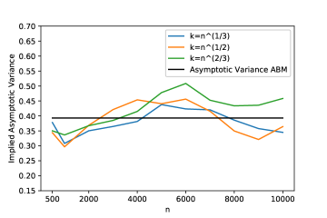
Figure 1: Implied Asymptotic Variance ABM Estimator, Student-t$(\nu=2)$

Second, we compare the single sample performance between the ABM estimator and the disjoint BM estimator. Figure 2 shows the plot of the estimates against various values of $k$ based on one single sample consisting of 10000 observations drawn from the Student-t($\nu=2$) distribution. Although both estimators are biased, the ABM estimator demonstrates a smoother path with respect to the change of $k$ than that of the disjoint BM estimator. The smooth path allows for an straightforward visual choice for the optimal $k$ in application.

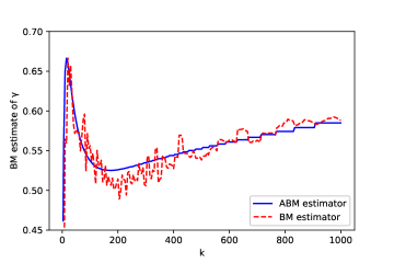
Figure 2: Single sample performance, Student-t$(\nu=2)$

Thirdly, we compare the performance of the ABM estimator to the disjoint BM estimator by plotting their Mean-Squared-Error (MSE) against various values of $k$ in Figure 3. We focus on the Student-t distribution with $\nu=2,3,4,5$ and sample size $n=1000$. For the Student-t distribution with $\nu=2$, we observe that the ABM estimator outperforms the disjoint BM estimator for almost all values of $k$. Such a superior performance of the ABM estimator is less obvious when the tail is less heavy (i.e. with a higher degrees of freedom). Nevertheless, for all four distributions, at the optimal $k$, the ABM estimator outperforms the disjoint BM estimator.

Figure 3: MSE for ABM and BM estimator

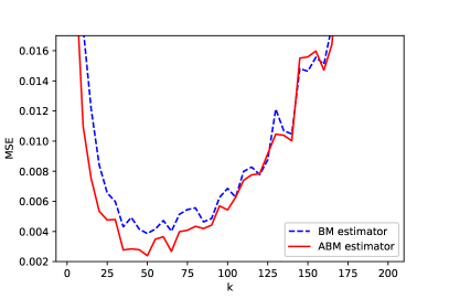
(a) Student-t ($\nu=2$)

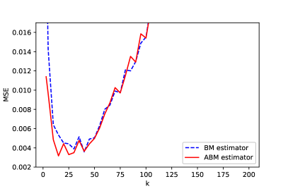
(b) Student-t ($\nu=3$)

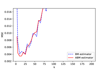
(c) Student-t ($\nu=4$)

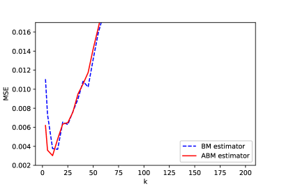
(d) Student-t ($\nu=5$)

To further understand the origin of the better performance of the ABM estimator, we decompose the MSE into bias and variance in Figure 4 and 5. We observe that regarding the bias, the disjoint BM estimator performs better. This is due to the fact that the ABM estimator involves potentially lower order statistics in the estimation. However, the ABM estimator performs better with a lower asymptotic variance. This is in line with the asymptotic theory. We further investigate the bias variance tradeoff. For $\nu=2$, the difference in bias is around 0.01, i.e. the squared bias is around 0.0001. However, the difference in variance is around 0.002, about 20 times higher than that in the squared bias. The variance thus plays a dominating role in the MSE. Hence, we conclude that the superior performance of the ABM estimator in terms of MSE stems from its lower variance. For distributions with higher degrees of freedom, the second order index $\rho=-2/\nu$ is closer to zero, which implies a higher bias in the estimators. As $\nu$ increases, the role of the bias becomes more important in the MSE comparison. In turn, the superior performance of the ABM estimator in terms of MSE is becomes less pronounced.

Figure 4: Bias for ABM and BM estimator

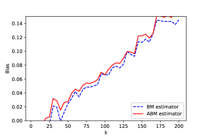
(a) Student-t ($\nu=2$)

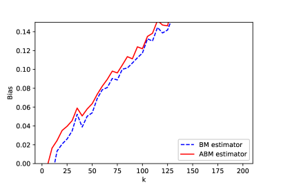
(b) Student-t ($\nu=3$)

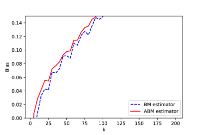
(c) Student-t ($\nu=4$)

(d) Student-t ($\nu=5$)

Figure 5: Variance for ABM and BM estimator

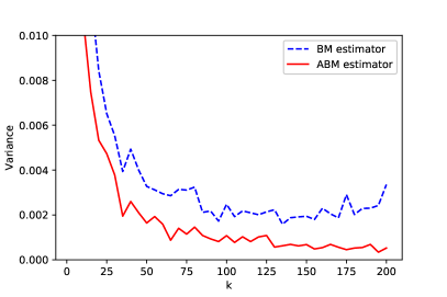
(a) Student-t ($\nu=2$)

(b) Student-t ($\nu=3$)

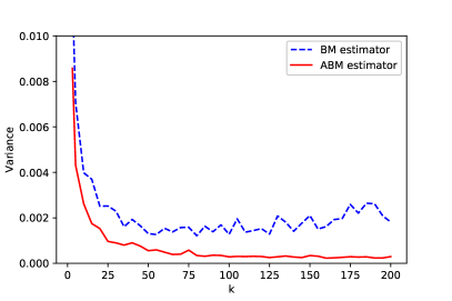
(c) Student-t ($\nu=4$)

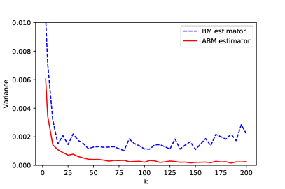
(d) Student-t ($\nu=5$)

Finally, we investigate other data generating processes. Figure 6 shows the MSE of the ABM estimator and disjoint BM estimator when drawing random samples from the Fréchet and Pareto distribution with shape parameter $\gamma=1/2$, and sample size $n=1000$. Different from the Student-t distributions which satisfies $\rho=\rho^{\prime}$, for these two distributions, the two second order parameters diverge; $\rho=-1$ and $\rho^{\prime}=-\infty$ for the Fréchet distribution and $\rho=-\infty$ and $\rho^{\prime}=-1$ for the Pareto distribution. We observe that for these two distributions, the MSE of the ABM estimator is generally below or at par with that of the disjoint BM estimator for the entire range of $k$. Note that for the Fréchet distribution we can eventually choose $k$ as high as the sample size $n$. When $k=n$, the ABM estimator coincides with the disjoint BM estimator.

Figure 6: MSE for ABM and BM estimator

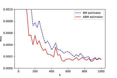
(a) Fréchet $(\gamma=1/2)$

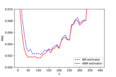
(b) Pareto $(\gamma=1/2)$

4.2 Non-i.i.d. Data Generating Processes

Although Theorem 3.5 is proved for i.i.d observations, here we explore the behaviour of the ABM estimator when the observations are serially dependent or are not identically distributed. We keep the number of simulations $m=100$ throughout.

4.2.1 Linear Serial Dependence

We introduce serial dependence by means of the AR(1) model,

$$X_{t}=\phi X_{t-1}+\epsilon_{t},\text{ for }t\geq 2$$ (4.1)

where we set $X_{1}=\epsilon_{1}$, $\{\epsilon_{t}\}_{t=1}^{\infty}$ is an i.i.d sequence following the Student-t(2) distribution and $\phi$ determines the degree of serial dependence. Note that for this model it holds that the extremal index $\theta=1-\phi^{4}$, see e.g. Chernick et al. (1991). For each value $\phi\in\{0.1,0.5,0.9\}$, we generate 2100 observations and then discard the first 100 observations. Hence the sample size is $n=2000$. We use the truncation constant $c=10^{-3}$.

The resulting MSE errors for both the ABM and BM estimator are displayed in Figure 7 for various levels of serial dependence. In all three cases, the ABM estimator outperforms the BM estimator at the optimal $k$. As $\phi$ increases, the MSE for both estimators increases. In the case of strongest dependence the ABM estimator performs considerably better than the BM estimator at the optimal $k$ and over a wide range of $k$ values.

Figure 7: MSE under serial dependence

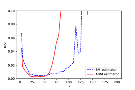
(a) $\phi=0.1$

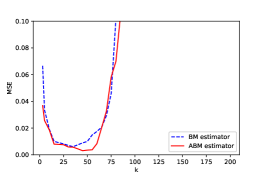
(b) $\phi=0.5$

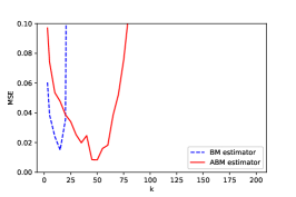
(c) $\phi=0.9$

4.2.2 GARCH Dependence

We simulate the observations from a GARCH$(1,1)$ model defined by

$$X_{t}=\sigma_{t}\epsilon_{t}$$

$$\sigma_{t}^{2}=\lambda_{0}+\lambda_{1}X_{t-1}^{2}+\lambda_{2}\sigma_{t-1}^{2}$$

where $\lambda_{1}+\lambda_{2}<1$ to ensure stationarity and $\epsilon_{t}$ is i.i.d. Student-t(6) distributed. As before, we generate $2100$ observations and discard the first $100$ to maintain a sample size $n=2000$. We use the same truncating constant $c=10^{-3}$.

In the GARCH model the tail behaviour of the observations $X_{t}$ is not directly inherited from $\epsilon_{t}$. Following Kesten (1973) we get that $\gamma=\frac{1}{2\kappa}$ where $\kappa$ is the solution of

$$\mathbb{E}\left(\lambda_{1}\epsilon_{t}^{2}+\lambda_{2}\right)^{\kappa}=1.$$

We fix $\lambda_{0}=0.5$, and consider the combinations $\{\lambda_{1}=0.11,\lambda_{2}=0.88\}$ and $\{\lambda_{1}=0.08,\lambda_{2}=0.91\}$, implying $\gamma\approx 0.35$ and $\gamma\approx 0.29$ respectively. These parameters combinations for $\lambda_{1}$ and $\lambda_{2}$ are close to parameters estimates obtained from financial data, see e.g. Sun and Zhou (2014). Figure 8 shows that the ABM method performs better than the disjoint BM method at the optimal $k$, but not for high values of $k$.

The overall better performance of the ABM estimator under both linear and GARCH serial dependence can be explained by the following heuristic. Under stationary serial dependence models such as the AR and GARCH models, the block maxima following the initial order of the observations often converges to the same GEV distribution as in the i.i.d. case, but with different normalization constants. Here the extreme value index $\gamma$ is the shape parameter in the GEV and the normalization constants are related to the extremal index. When considering all block maxima, the order of the observations and the serial dependence structure are discarded. In turn, the all block maxima can be regarded as similar to those of an i.i.d. sequence drawn from the stationary distribution, which has the same limiting GEV distribution with the same shape paramter $\gamma$. Therefore, once fitting the all block maxima to a three-parameter GEV distribution (or a two-parameter GEV distribution in case $\gamma>0$), the estimator for the shape parameter, i.e. $\gamma$, remains valid. It benefits from a reduced estimation variance as in the i.i.d. case. This explains the observed superior performance of the ABM estimator for serially dependent data. However, we remark that the corresponding estimator of the scale is not a valid estimator for the scale of the block maxima under serial dependence. If one intends to use the scale estimator from the ABM procedure for estimating other quantities such as the return level, a proper transformation involving the extremal index is needed.

Figure 8: MSE under GARCH

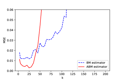
(a) $\lambda_{1}=0.08,\lambda_{2}=0.91$

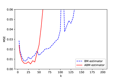
(b) $\lambda_{1}=0.11,\lambda_{2}=0.88$

4.2.3 Scale Heterogeneity

We introduce scale heterogeneity by generating the observations as

$$X_{t}=\begin{cases}r\left|\epsilon_{t}\right|\text{ if }t>n/2\\ \left|\epsilon_{t}\right|\text{ if }t\leq n/2\end{cases}$$

where $\{\epsilon_{t}\}$ is an i.i.d. series following the Student-t(2) distribution. We use $r\in\{2,5\}$ to distinguish low and high scale heterogeneity. The sample size is $n=1000$. Figure 9 illustrates that the ABM strongly outperforms the disjoint BM method under scale heterogeneity. The superior performance is more evident when heterogeneity in scale is higher.

Figure 9: MSE under Scale Heterogeneity

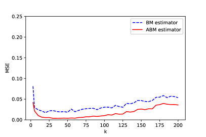
(a) $r=2$

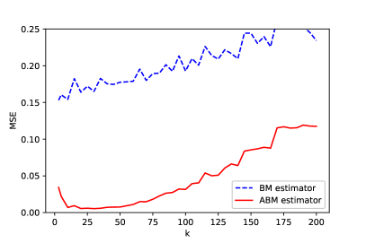
(b) $r=5$

5 Proofs

5.1 Preliminaries

Recall that we use the weights $p_{i}=\binom{n-i}{m-1}/\binom{n}{m}$ to reweigh the truncated order statistic $X^{c}_{n-i+1:n}$. The following lemma shows that these weights are uniformly close to $q_{i}=\frac{1}{k}e^{-(i-1)/k}$.

Lemma 5.1

Under Condition 3.3 we have that for any $d>0$

$$\frac{p_{i}}{\frac{1}{k}e^{-(i-1)/k}}-1=(\log k)^{4d}\left(\frac{1}{k}+\frac{1}{m}\right)O(1),$$ (5.1)

holds uniformly for $1\leq i\leq k(\log k)^{d}$, as $n\to\infty$

Proof. Clearly, the lemma holds for $i=1$. For $i\geq 2$, we can write the binomial weight $p_{i}$ as

$$p_{i}=\frac{1}{k}\left(\frac{n-m}{n-1}\right)^{i-1}\prod_{j=1}^{i-2}\frac{1-\frac{j}{n-m}}{1-\frac{j}{n-1}},$$

which leads to

$$\log\frac{p_{i}}{\frac{1}{k}e^{-(i-1)/k}}=-(i-1)\left(\frac{1}{k}-\log\frac{n-m}{n-1}\right)+\sum_{j=1}^{i-2}\log\frac{1-\frac{j}{n-m}}{1-\frac{j}{n-1}}=:I_{1}+I_{2}.$$

For $I_{1}$, clearly, as $n\to\infty$, uniformly for all $i\leq k(\log k)^{d}$

$$\left|I_{1}\right|\leq k(\log k)^{d}\left(\frac{1}{k}-\log\left(1-\frac{1-m}{n-1}\right)\right)=\frac{(\log k)^{d}}{k}O(1).$$

Next we handle $I_{2}$. By Condition 3.3, for all $j<i\leq k(\log k)^{d}$ we have uniformly, $j/(n-1)\leq j/(n-m)=\frac{(\log k)^{d}}{m}O(1)\to 0$ as $n\to\infty$. Thus

$$\log\frac{1-\frac{j}{n-m}}{1-\frac{j}{n-1}}$$

$$= -\left(\frac{j}{n-m}\right)-\left(\frac{j}{n-m}\right)^{2}+O\left(\left(\frac{j}{n-m}\right)^{3}\right)+\left(\frac{j}{n-1}\right)+\left(\frac{j}{n-1}\right)^{2}+O\left(\left(\frac{j}{n-1}\right)^{3}\right)$$

$$= -\frac{j(m-1)}{(n-1)(n-m)}-\frac{j(m-1)}{(n-1)(n-m)}\left(\frac{j}{n-m}+\frac{j}{n-1}\right)+\left(\frac{j}{n}\right)^{3}O(1)$$

$$= \frac{j}{nk}O(1)+\left(\frac{j}{n}\right)^{3}O(1),$$

where the $O(1)$ terms are uniform for all $j<i\leq k(\log k)^{d}$ as $n\to\infty$. By aggregating these terms we get that, uniform for all $i\leq k(\log k)^{d}$ as $n\to\infty$,

$$I_{2}= \sum_{j=1}^{i-2}\log\frac{1-\frac{j}{n-m}}{1-\frac{j}{n-1}}=\sum_{j=1}^{i-2}\left(\frac{j}{nk}O(1)+\left(\frac{j}{n}\right)^{3}O(1)\right)$$

$$= \frac{1}{nk}(k(\log k)^{d})^{2}O(1)+\frac{(k(\log k)^{d})^{4}}{n^{3}}O(1)$$

$$= \frac{(\log k)^{2d}}{m}O(1)+\frac{k(\log k)^{4d}}{m^{3}}O(1)$$

By Condition 3.3, we get that $k=o(n^{2/3})$, which implies that $k/m^{2}\to 0$ as $n\to\infty$. Hence, as $n\to\infty$, $I_{2}=\frac{(\log k)^{4d}}{m}O(1)$. The lemma is proved by combining $I_{1}$ and $I_{2}$.   

In the proof of Proposition 3.6, we need to replace the deterministic term $\frac{n}{k}\left(1-F(x\sigma_{m})\right)$ by its limit $x^{-1/\gamma}$. The following lemma shows that such a replacement is allowed for a wide range of $x$ uniformly.

Lemma 5.2

Assume that conditions 3.1 and 3.3 hold for some $\rho<0$. For any $\delta>0$, there exists $c_{1}=c_{1}(\delta,\rho,\gamma,\epsilon)>0$ such that as $n\to\infty$,

$$\sup_{x>\left(\log k\right)^{-\delta}}x^{\frac{1/2-\epsilon}{\gamma}}\left|\frac{n}{k}\left(1-F\left(\sigma_{m}x\right)\right)-x^{-1/\gamma}\right|=O\left(a(\sigma_{m})(\log k)^{c_{1}}\right)\to 0$$ (5.2)

In addition, there exists $c_{3}=c_{3}(\delta,\rho,\gamma)>0$ such that as $n\to\infty$,

$$\sup_{x>\left(\log k\right)^{-\delta}}\left|\frac{\frac{n}{k}\left(1-F(x\sigma_{m})\right)}{x^{-1/\gamma}}-1\right|=O\left(a(\sigma_{m})(\log k)^{c_{3}}\right)\to 0.$$ (5.3)

Proof. Convergence of the right hand sides of (5.2)-(5.3) to zero follows by Condition 3.3. Thus, we only show the statements regarding the order.

Recall the inequality in (3.3). Since $\sigma_{m}\left(\log k\right)^{-\delta}\to\infty$ as $n\to\infty$, we get that for any $\delta,\delta^{\prime},\epsilon>0$, there exists $n(\delta,\delta^{\prime},\epsilon)$ such that for all $n>n(\delta,\delta^{\prime},\epsilon)$ and $x>\left(\log k\right)^{-\delta}$,

$$\left|\frac{\frac{n}{k}\left(1-F(x\sigma_{m})\right)}{x^{-1/\gamma}}-1\right|\leq\left|a(\sigma_{m})\right|\left(\epsilon{x}^{\rho/\gamma}\max\left({x}^{\delta^{\prime}},{x}^{-\delta^{\prime}}\right)+\frac{x^{\rho/\gamma}-1}{\rho\gamma}\right).$$ (5.4)

From (5.4), we obtain that for all $n>n(\delta,\delta^{\prime},\epsilon)$ and $x>(\log k)^{-\delta}$,

$$x^{\frac{1/2-\epsilon}{\gamma}}\left|\frac{n}{k}\left(1-F(x\sigma_{m})\right)-x^{-1/\gamma}\right|\leq\left|a(\sigma_{m})\right|x^{\frac{-1/2+\epsilon}{\gamma}}\left(\epsilon{x}^{\rho/\gamma}\max\left({x}^{\delta^{\prime}},{x}^{-\delta^{\prime}}\right)+\frac{x^{\rho/\gamma}-1}{\rho\gamma}\right).$$

By choosing $\delta^{\prime}$ such that $\delta^{\prime}<(-\rho+1/2+\epsilon)/\gamma$ we get that, for all $x>(\log k)^{-\delta}$,

$$x^{-\frac{1/2+\epsilon}{\gamma}}\left(\epsilon{x}^{\rho/\gamma}\max\left({x}^{\delta^{\prime}},{x}^{-\delta^{\prime}}\right)+\frac{x^{\rho/\gamma}-1}{\rho\gamma}\right)<(\log k)^{c_{1}},$$

with $c_{1}>2\delta(-\rho+1/2+\epsilon)/\gamma$, which completes the proof of (5.2).

Equation (5.3) is proved in a similar way by directly handling the right hand side of (5.4): now choose $\delta^{\prime}<-\rho/\gamma$ and $c_{3}>-2\delta\rho/\gamma$.

 

Finally, to prove Proposition 3.6 we extend Theorem 5.1.4 in de Haan and Ferreira (2006) as in the lemma presented below. The extension concerns two different aspects. Firstly, in contrast to a fixed lower bound on the range of $x$, we allow the lower bound to go to zero at a logarithmic speed. Secondly, we have an additional rate $k^{\epsilon^{*}}$ in the limit result.

Lemma 5.3

Under Conditions 3.1, 3.3 for any $\delta>0$ and any $0<\epsilon<1/2$ there exists $\epsilon^{*}=\epsilon^{*}(l,\rho,\epsilon)$ such that as $n\to\infty$,

$$\sup_{x>\left(\log k\right)^{-\delta}}k^{\epsilon^{*}}x^{\frac{1/2-\epsilon}{\gamma}}\left|\sqrt{k}\left(\frac{n}{k}\left(1-F_{n}(\sigma_{m}x)\right)-x^{-1/\gamma}\right)-W_{n}\left(x^{-1/\gamma}\right)\right|\overset{P}{\to}0,$$ (5.5)

where $F_{n}(x)=\frac{1}{n}\sum_{i=1}^{n}\mathbb{I}\{X_{i}\leq x\}$.

Proof. We start from Corollary 3.2, Ch. $4.3$ in Csörgö and Horváth (1993). Consider the uniform empirical distribution function, $U_{n}(t):=\frac{1}{n}\sum_{i=1}^{n}\mathbb{I}\{U_{i}\leq t\}$, where $U_{1},U_{2},\ldots$ are i.i.d. standard uniform random variables. Then there exists a sequence of Brownian Bridges $B_{n}$ such that for all $0<\nu<1/2$ as $n\to\infty$,

$$n^{1/2-\nu}\sup_{0<t<1}\frac{\left|\sqrt{n}(U_{n}(t)-t)-B_{n}(t)\right|}{(t(1-t))^{\nu}}=O_{p}(1).$$

By replacing $t$ with $t\frac{k}{n}$, we get that as $n\to\infty$,

$$k^{1/2-\nu}\sup_{0<t<\frac{n}{k}}t^{-\nu}\frac{\left|\sqrt{k}\left(\frac{n}{k}U_{n}\left(t\frac{k}{n}\right)-t\right)-\frac{\sqrt{n}}{\sqrt{k}}B_{n}\left(t\frac{k}{n}\right)\right|}{\left(1-t\frac{k}{n}\right)^{\nu}}=O_{p}\left(1\right).$$

Let $z_{n}\left(x\right)=\frac{n}{k}\left(1-F\left(\sigma_{m}x\right)\right)$, then $z_{n}(x)<\frac{1}{2}\frac{n}{k}$ for sufficiently large $n$ when $x>(\log k)^{-\delta}$ because $\sigma_{m}(\log k)^{-\delta}\to\infty$. By taking $t=z_{n}(x)$ and $\nu=1/2-\epsilon$ we obtain that for any $\epsilon^{*}<\epsilon$, as $n\to\infty$,

$$k^{\epsilon^{*}}\sup_{x>(\log k)^{-\delta}}z_{n}\left(x\right)^{-1/2+\epsilon}\left|\sqrt{k}\left(\frac{n}{k}\left(1-F_{n}(\sigma_{m}x)\right)-z_{n}(x)\right)-\frac{\sqrt{n}}{\sqrt{k}}B_{n}\left(z_{n}(x)\frac{k}{n}\right)\right|\overset{P}{\to}0.$$ (5.6)

We intend to substitute the three $z_{n}(x)$ terms, referred to by order of appearance in (5.6) as the first, second and third $z_{n}(x)$ term below, by its limit $x^{-1/\gamma}$ for all $x>(\log k)^{-\delta}$ uniformly.

The first $z_{n}\left(x\right)$ term can be substituted by its limit $x^{-1/\gamma}$ uniformly for all $x>(\log k)^{-\delta}$ by (5.3). Hence, we have as $n\to\infty$,

$$k^{\epsilon^{*}}\sup_{x>(\log k)^{-\delta}}x^{\frac{1/2-\epsilon}{\gamma}}\left|\sqrt{k}\left(\frac{n}{k}\left(1-F_{n}\left(\sigma_{m}x\right)\right)-z_{n}(x)\right)-\frac{\sqrt{n}}{\sqrt{k}}B_{n}\left(z_{n}(x)\frac{k}{n}\right)\right|\overset{P}{\to}0.$$

Next, to handle the second $z_{n}(x)$ term, we need to show that as $n\to\infty$,

$$\lim_{n\to\infty}k^{\epsilon^{*}}\sup_{x>\left(\log k\right)^{-\delta}}x^{\frac{1/2-\epsilon}{\gamma}}\sqrt{k}\left|z_{n}(x)-x^{-1/\gamma}\right|=0.$$

This relation follows directly from (5.2) and Condition 3.3: as $n\to\infty$,

$$k^{\epsilon^{*}}\sup_{x>\left(\log k\right)^{-\delta}}x^{\frac{1/2-\epsilon}{\gamma}}\sqrt{k}\left|z_{n}(x)-x^{-1/\gamma}\right|=k^{1/2+\epsilon^{*}}a(\sigma_{m})(\log k)^{c_{1}}O(1)\to 0.$$

Here the last step follows by choosing $0<\epsilon^{*}<-\rho-l(1/2-\rho)$. The existence of such a positive constant $\epsilon^{*}$ is guaranteed by Condition 3.3, while the limit relation follows from the fact that $\left|a(\sigma_{m})\right|<\left(\frac{n}{k}\right)^{\rho+\epsilon^{*}}$ for sufficiently large $n$, see Remark 3.4.

Lastly, we handle the third $z_{n}(x)$ term. Write $B_{n}(u)=\tilde{W}_{n}(u)-u\tilde{W}_{n}(1)$, where $\tilde{W}_{n}$ is a properly defined Brownian motion. Further define $W_{n}(u)=\sqrt{\frac{n}{k}}\tilde{W}_{n}\left(\frac{k}{n}u\right)$. Then $W_{n}(u)$ is also a Brownian motion and $\sqrt{\frac{n}{k}}B_{n}\left(z_{n}(x)\frac{k}{n}\right)=W_{n}\left(z_{n}(x)\right)-\sqrt{\frac{k}{n}}z_{n}(x)\tilde{W}_{n}(1)$. We shall prove that, as $n\to\infty$,

$$k^{\epsilon^{*}}\sup_{x>\left(\log k\right)^{-\delta}}x^{\frac{1/2-\epsilon}{\gamma}}\left|W_{n}(z_{n}(x))-W_{n}\left(x^{-1/\gamma}\right)\right|=o_{p}(1),$$ (5.7)

$$k^{\epsilon^{*}}\sup_{x>\left(\log k\right)^{-\delta}}x^{\frac{1/2-\epsilon}{\gamma}}\left|z_{n}(x)\sqrt{\frac{k}{n}}\tilde{W}_{n}(1)\right|=o_{p}(1).$$ (5.8)

We prove Equation (5.7) by splitting the region $\{x>\left(\log k\right)^{-\delta}\}$ into two regions $\{\left(\log k\right)^{-\delta}<x<x_{0}\}$ and $\{x\geq x_{0}\}$ for a fixed constant $x_{0}$.

The region $\{x\geq x_{0}\}$ can be dealt with by the Levy’s modulus of continuity for Brownian motion in the following form (see Theorem 1.1.1 and its colloraries in Csörgo and Révész (2014)):

$$\lim_{h\to 0}\sup_{0\leq s\leq b}\frac{\left|W(s+h)-W(s)\right|}{\sqrt{2h\log(1/h)}}\overset{a.s.}{=}1,$$

where $W(\cdot)$ is a generic Brownian Motion and any fixed $b<\infty$.

By (5.2), we get uniformly for all $x\geq x_{0}$ that $\left|z_{n}(x)-x^{-1/\gamma}\right|\to 0$ as $n\to\infty$. Consequently, for sufficiently large $n$, almost surely

$$\sup_{x\geq x_{0}}x^{\frac{1/2-\epsilon}{\gamma}}\left|W(z_{n}(x))-W(x^{-1/\gamma})\right|\leq 2\sup_{x\geq x_{0}}x^{\frac{1/2-\epsilon}{\gamma}}\left|z_{n}(x)-x^{-1/\gamma}\right|^{1/2-\epsilon}.$$

By Condition 3.3 and (5.3), we get that as $n\to\infty$,

$$k^{\epsilon^{*}}\sup_{x\geq x_{0}}x^{\frac{1/2-\epsilon}{\gamma}}\left|{W}({z_{n}}({x}))-W\left(x^{-1/\gamma}\right)\right|=k^{\epsilon^{*}}a(\sigma_{m})^{1/2-\epsilon}(\log k)^{c_{3}(1/2-\epsilon)}O(1)\to 0\text{ a.s. }$$

by choosing $\epsilon^{*}<-\rho/l(1/2-\epsilon)+\rho(1/2-\epsilon)$. Therefore, to prove (5.7) it is left to handle the region $\{\left(\log k\right)^{-\delta}<x<x_{0}\}$, i.e. as $n\to\infty$,

$$k^{\epsilon^{*}}\sup_{(\log k)^{-\delta}<x\leq x_{0}}x^{\frac{1/2-\epsilon}{\gamma}}\left|W_{n}(z_{n}(x))-W_{n}\left(x^{-1/\gamma}\right)\right|\overset{P}{\to}0.$$ (5.9)

Define $V_{n}(t)=tW_{n}(1/t)$. Then $V_{n}(t)$ is also a Brownian Motion. We bound the left hand side of Equation (5.9) as follows:

$$k^{\epsilon^{*}}x^{\frac{1/2-\epsilon}{\gamma}}\left|W_{n}(z_{n}(x))-W_{n}\left(x^{-1/\gamma}\right)\right|$$

$$= k^{\epsilon^{*}}x^{\frac{1/2-\epsilon}{\gamma}}\left|\frac{z_{n}(x)}{x^{-1/\gamma}}x^{-1/\gamma}V_{n}\left(\frac{1}{z_{n}(x)}\right)-x^{-1/\gamma}V_{n}\left(x^{1/\gamma}\right)\right|$$

$$\leq k^{\epsilon^{*}}x^{\frac{-1/2-\epsilon}{\gamma}}\left(\left|V_{n}\left(\frac{1}{z_{n}(x)}\right)\left(\frac{z_{n}(x)}{x^{-1/\gamma}}-1\right)\right|+\left|V_{n}\left(\frac{1}{z_{n}(x)}\right)-V_{n}(x^{1/\gamma})\right|\right)$$

$$=: \mathbb{I}_{1}(x)+\mathbb{I}_{2}(x).$$

To handle $\mathbb{I}_{1}(x)$, write

$$\mathbb{I}_{1}(x) =z_{n}(x)^{1/2-\epsilon}\left|V_{n}\left(\frac{1}{z_{n}(x)}\right)\right|\cdot\left(\frac{x^{-1/\gamma}}{z_{n}(x)}\right)^{1/2-\epsilon}\cdot k^{\epsilon^{*}}x^{-2\epsilon/\gamma}\left|\frac{z_{n}(x)}{x^{-1/\gamma}}-1\right|$$

$$=:\mathbb{I}_{11}(x)\cdot\mathbb{I}_{12}(x)\cdot\mathbb{I}_{13}(x).$$

For $(\log k)^{-\delta}<x<x_{0}$, (5.3) implies that for sufficiently large $n$, $\frac{1}{z_{n}(x)}<2x_{0}^{1/\gamma}$ uniformly and as $n\to\infty$, $\mathbb{I}_{12}(x)=O(1)$. As $n\to\infty$, since $\sup_{s<2x_{0}^{1/\gamma}}s^{-1/2+\epsilon}\left|V_{n}(s)\right|=O_{p}(1)$ , we conclude that $\mathbb{I}_{11}(x)=O_{p}(1)$ uniformly for all $(\log k)^{-\delta}<x<x_{0}$. Finally, for $\mathbb{I}_{13}(x)$, (5.3) implies that as $n\to\infty$,

$$\sup_{(\log k)^{-\delta}<x<x_{0}}\mathbb{I}_{13}(x)\leq k^{\epsilon^{*}}\sup_{(\log k)^{-\delta}<x<x_{0}}x^{-2\epsilon/\gamma}\sup_{(\log k)^{-\delta}<x<x_{0}}\left|\frac{z_{n}(x)}{x^{-1/\gamma}}-1\right|$$

$$= k^{\epsilon^{*}}a(\sigma_{m})(\log k)^{c_{3}+2\delta\epsilon/\gamma}O(1)=o(1),$$

where the $o(1)$ term in the last equality follows by Condition 3.3 and choosing $\epsilon^{*}<-\rho/l+\rho$. Combining the three components, we conclude that as $n\to\infty$,

$$\sup_{(\log k)^{-\delta}<x<x_{0}}\mathbb{I}_{1}(x)=o_{p}(1).$$

We handle $\mathbb{I}_{2}(x)$ by applying the modulus of continuity to the Brownian Motion $V_{n}(\cdot)$. From (5.3), we get that as $n\to\infty$,

$$\sup_{\left(\log k\right)^{-\delta}<x\leq x_{0}}\left|\frac{1}{z_{n}(x)}-\frac{1}{x^{-1/\gamma}}\right|=\sup_{\left(\log k\right)^{-\delta}<x\leq x_{0}}\frac{1}{z_{n}(x)}\left|\frac{z_{n}(x)}{x^{-1/\gamma}}-1\right|=O(1)o(1)=o(1),$$

Thus, we can apply the modulus of continuity as intended. The rest of the proof is similar to that for the region $\{x>x_{0}\}$. By combining the two components $\mathbb{I}_{1}(x)$ and $\mathbb{I}_{2}(x)$, we conclude that (5.9), and thereby (5.7), is proved.

Finally, by choosing $\epsilon^{*}<1/4$, (5.8) is proved by combining Condition 3.3 with the following facts: as $n\to\infty$, $k^{3/2}/\sqrt{n}\to 0$, $\tilde{W}_{n}(1)=O_{p}(1)$, ${z_{n}}({x})/x^{-1/\gamma}=O(1)$ and $\sup_{x>\left(\log k\right)^{-\delta}}x^{\frac{-1/2-\varepsilon}{\gamma}}=O\left((\log(k))^{\delta(1/2+\varepsilon)/\gamma}\right)$.

 

5.2 Proof of Proposition 3.6

Proof of Proposition 3.6. We shall prove the proposition in three steps: as $n\to\infty$,

$$\sup_{x>\left(\log k\right)^{-\delta}}k^{\tilde{\epsilon}}x^{\frac{1/2-\epsilon}{\gamma}}\sqrt{k}\left(\mathbb{P}_{n}(x)-\mathbb{P}_{n}^{1}(x)\right)=o_{p}(1),$$ (5.10)

$$\sup_{x>\left(\log k\right)^{-\delta}}k^{\tilde{\epsilon}}x^{\frac{1/2-\epsilon}{\gamma}}\sqrt{k}\left(\mathbb{P}_{n}^{1}(x)-\mathbb{P}_{n}^{2}(x)\right)=o_{p}(1),$$ (5.11)

$$\sup_{x>\left(\log k\right)^{-\delta}}k^{\tilde{\epsilon}}x^{\frac{1/2-\epsilon}{\gamma}}\left|\sqrt{k}\left(\mathbb{P}_{n}^{2}(x)-\left(1-e^{-x^{-1/\gamma}}\right)\right)-e^{-x^{-1/\gamma}}W_{n}(x^{-1/\gamma})\right|=o_{p}(1),$$ (5.12)

where

$$\mathbb{P}_{n}^{(1)}(x)=\sum_{i=1}^{n-m+1}\frac{1}{k}e^{-(i-1/k)}\mathbb{I}\{\frac{X^{c}_{n-i+1:n}}{\sigma_{m}}>x\},$$

$$\mathbb{P}_{n}^{(2)}(x)=\sum_{i=1}^{n}\frac{1}{k}e^{-(i-1/k)}\mathbb{I}\{\frac{X^{c}_{n-i+1:n}}{\sigma_{m}}>x\}.$$

Compared to $\mathbb{P}_{n}$, $\mathbb{P}_{n}^{(1)}$ uses the weights $q_{i}$ instead of $p_{i}$ and $\mathbb{P}_{n}^{(2)}$ further includes the lowest $m-1$ order statistics.

Denote $\bar{F}_{n}(x)=\frac{1}{n}\sum_{i=1}^{n}\mathbb{I}\{X_{i}>x\}$. Note that for sufficiently large $n$ we have $\sigma_{m}x>c$ for all $x>\left(\log k\right)^{-\delta}$, which implies $\{X^{c}_{n-i+1:n}>\sigma_{m}x\}=\{\bar{F}_{n}(\sigma_{m}x)\geq\frac{i}{n}\}$ holds for all $1\leq i\leq n-m+1$ and $x>\left(\log k\right)^{-\delta}$. Consequently, we get that for sufficiently large $n$,

$$k^{\tilde{\epsilon}}x^{\frac{1/2-\epsilon}{\gamma}}\sqrt{k}\ \left|\mathbb{P}_{n}(x)-\mathbb{P}_{n}^{(1)}(x)\right|$$

$$\leq k^{\tilde{\epsilon}}x^{\frac{1/2-\epsilon}{\gamma}}\sqrt{k}\sum_{i=1}^{n-m+1}\left|p_{i}-\frac{1}{k}e^{-(i-1)/k}\right|\ \mathbb{I}\{X^{c}_{n-i+1:n}>\sigma_{m}x\}$$

$$= k^{\tilde{\epsilon}}x^{\frac{1/2-\epsilon}{\gamma}}\sqrt{k}\sum^{n\bar{F}_{n}(x\sigma_{m})}_{i=1}\frac{1}{k}e^{-(i-1)/k}\left|\frac{p_{i}}{q_{i}}-1\right|.$$

We intend to apply Lemma 5.1 to bound the terms $\left|\frac{p_{i}}{q_{i}}-1\right|$ for $i\leq n\bar{F}_{n}(x\sigma_{m})$. Notice that Lemma 5.3 implies that, for any $\eta>0$ and sufficiently large $n$, on a set $A_{n}$ with $\mathbb{P}(A_{n})>1-\eta$ we have

$$n\bar{F}_{n}(\sigma_{m}(\log k)^{-\delta})\leq k^{1/2-\epsilon^{*}}(\log k)^{\delta\left(\frac{1/2-\epsilon}{\gamma}\right)}+\sqrt{k}\left|W_{n}\left((\log k)^{\frac{\delta}{\gamma}}\right)\right|+k(\log k)^{\delta/\gamma}.$$

$$\leq k(\log k)^{d},$$

where $d>\delta/\gamma$. Hence by Lemma 5.1 we obtain that for sufficiently large $n$, on the set $A_{n}$, there exists a constant $C$ such that

$$k^{\tilde{\epsilon}}x^{\frac{1/2-\epsilon}{\gamma}}\sqrt{k}\left|\mathbb{P}_{n}(x)-\mathbb{P}_{n}^{1}(x)\right|$$

$$\leq C\left((\log k)^{4d}\left(\frac{1}{k}+\frac{1}{m}\right)\right)k^{\tilde{\epsilon}}x^{\frac{1/2-\epsilon}{\gamma}}\sqrt{k}\sum^{n\bar{F}_{n}(x\sigma_{m})}_{i=1}\frac{1}{k}e^{-(i-1)/k}$$

$$= C\left((\log k)^{4d}\left(\frac{1}{k}+\frac{1}{m}\right)\right)k^{\tilde{\epsilon}}x^{\frac{1/2-\epsilon}{\gamma}}\sqrt{k}\left(1-e^{-\frac{n}{k}\bar{F}_{n}\left(\sigma_{m}x\right)}\right),$$

uniformly for $x>\left(\log k\right)^{-\delta}$. By the taylor expansion of the function $\phi(y)=1-e^{-y}$ at the point $x^{-1/\gamma}$, we obtain that, there exists $\tilde{x}_{n}$ between $x^{-1/\gamma}$ and $\frac{n}{k}\bar{F}_{n}(\sigma_{m}x)$ such that

$$x^{\frac{1/2-\epsilon}{\gamma}}\left(1-e^{-\frac{n}{k}\bar{F}_{n}(\sigma_{m}x)}\right)=x^{\frac{1/2-\epsilon}{\gamma}}(1-e^{-x^{-1/\gamma}})+x^{\frac{1/2-\epsilon}{\gamma}}e^{-\tilde{x}_{n}}\left(\frac{n}{k}\bar{F}_{n}(\sigma_{m}x)-x^{-1/\gamma}\right).$$

Note that $\sup_{x>0}x^{\frac{1/2-\epsilon}{\gamma}}\left(1-e^{-x^{-1/\gamma}}\right)$ is finite. Together with the fact that $0<e^{-\tilde{x_{n}}}<1$ and Lemma 5.3, we conclude that $\sup_{x>(\log k)^{-\delta}}x^{\frac{1/2-\epsilon}{\gamma}}\left(1-e^{-\frac{n}{k}\bar{F}_{n}(\sigma_{m}x)}\right)=O_{p}(1)$. By Condition 3.3, $k=O(n^{l})$ with $l<2/3$. Therefore we can take $\tilde{\epsilon}<1/l-3/2$ small enough and have that $k^{1/2+\tilde{\epsilon}}(\log k)^{4d}/m\to 0$. With this $\tilde{\epsilon}$ we conclude that (5.10) is proved.

To prove (5.11), note that $\{\left|\mathbb{P}_{n}^{1}(x)-\mathbb{P}_{n}^{2}(x)\right|\neq 0\}\subset\{X^{c}_{m:n}>\sigma_{m}x\}$. Moreover, for any constant $0<a<1$ we have eventually $X_{m:n}\leq X_{na:n}$ while $X_{na:n}\overset{P}{\to}F^{-1}(a)<\infty$ and $\left(\log k\right)^{-\delta}\sigma_{m}\to\infty$, as $n\to\infty$. Therefore $\mathrm{P}\left(X_{m:n}^{c}>\sigma_{m}x\right)\to 0$ as $n\to\infty$, which proves (5.11).

To prove (5.12), recall the equivalence between the events $\{X^{c}_{n-i+1:n}>\sigma_{m}x\}$ and $\{\bar{F}_{n}(\sigma_{m}x)\geq\frac{i}{n}\}$ for large enough $n$ and $\phi(y)=1-e^{-y}$. Write

$$\mathbb{P}_{n}^{(2)}(x)= \sum_{i=1}^{n}\frac{1}{k}e^{-(i-1)/k}\mathbb{I}\{\frac{X^{c}_{n-i+1:n}}{\sigma_{m}}>x\}$$

$$= \sum_{i=1}^{n}\frac{1}{k}{e}^{-({i}-1)/k}\mathbb{I}\{\bar{F}_{n}(\sigma_{m}x)\geq\frac{i}{n}\}$$

$$= \sum^{n\bar{F}_{n}(\sigma_{m}x)}_{i=1}\frac{1}{k}e^{-(i-1)/k}=\frac{1-e^{-\frac{n}{k}\bar{F}_{n}(\sigma_{m}x)}}{k(1-e^{-1/k})}=\left(1+\frac{1}{k}o(1)\right)\phi\left(\frac{n}{k}\bar{F}_{n}(\sigma_{m}x)\right).$$

Since

$$\phi\left(\frac{n}{k}\bar{F}_{n}\left(\sigma_{m}x\right)\right)-\phi\left(x^{-1/\gamma}\right)=e^{-x^{-1/\gamma}}\left(\frac{n}{k}\bar{F}_{n}(\sigma_{m}x)-x^{-1/\gamma}\right)-\frac{e^{-\tilde{x}_{n}}}{2}\left(\frac{n}{k}\bar{F}_{n}(\sigma_{m}x)-x^{-1/\gamma}\right)^{2},$$

where $\tilde{x}_{n}$ is in between $x^{-1/\gamma}$ and $\frac{n}{k}\bar{F}_{n}(\sigma_{m}x)$, by Lemma 5.3 we obtain that as $n\to\infty$,

$$\sup_{x\geq\left(\log k\right)^{-\delta}}x^{\frac{1/2-\epsilon}{\gamma}}\sqrt{k}\left(\frac{n}{k}\bar{F}_{n}(\sigma_{m}x)-x^{-1/\gamma}\right)=O_{p}(1).$$

By choosing $\tilde{\epsilon}<1/2$ we get that as $n\to\infty$,

$${k}^{\tilde{\epsilon}}\sup_{x\geq\left(\log k\right)^{-\delta}}x^{\frac{1/2-\epsilon}{\gamma}}\sqrt{k}\left(\frac{n}{k}\bar{F}_{n}(\sigma_{m}x)-x^{-1/\gamma}\right)^{2}=o_{p}(1).$$

Combining the aforementioned limit relations with the fact that $0<e^{-\tilde{x}_{n}}<1$, we get that as $n\to\infty$, uniformly for all $x>(\log k)^{-\delta}$,

$$\phi\left(\frac{n}{k}\bar{F}_{n}(\sigma_{m}x)\right)=\phi\left(x^{-1/\gamma}\right)+ e^{-x^{-1/\gamma}}\left(\frac{n}{k}\bar{F}_{n}\left(\sigma_{m}x)\right)-x^{-1/\gamma}\right)+k^{-1/2-\tilde{\epsilon}}x^{\frac{-1/2+\epsilon}{\gamma}}o_{p}(1)$$

$$=\phi\left(x^{-1/\gamma}\right)+ e^{-x^{-1/\gamma}}\left(k^{-1/2}W_{n}\left(x^{-1/\gamma}\right)+k^{-1/2-\epsilon^{*}}x^{\frac{-1/2+\epsilon}{\gamma}}o_{p}(1)\right)$$

$$+ k^{-1/2-\tilde{\epsilon}}x^{\frac{-1/2+\epsilon}{\gamma}}o_{p}(1)$$

$$=\phi\left(x^{-1/\gamma}\right)+ k^{-1/2}e^{-x^{-1/\gamma}}W_{n}\left(x^{-1/\gamma}\right)+k^{-1/2-\tilde{\epsilon}}x^{\frac{-1/2+\epsilon}{\gamma}}o_{p}(1),$$ (5.13)

where in the last step we choose $\tilde{\epsilon}<\epsilon^{*}$.

Since $\sup_{x>(\log k)^{-\delta}}x^{\frac{1/2-\epsilon}{\gamma}}e^{-x^{-1/\gamma}}W_{n}(x^{-1/\gamma})=O_{p}(1)$, as $n\to\infty$, and $\sup_{x>(\log k)^{-\delta}}x^{\frac{1/2-\epsilon}{\gamma}}\phi(x^{-1/\gamma})$ is finite, the relation (5.13) further implies that

$$\phi\left(\frac{n}{k}\bar{F}_{n}(\sigma_{m}x)\right)=x^{\frac{-1/2+\epsilon}{\gamma}}O(1)+k^{-1/2}x^{\frac{-1/2+\epsilon}{\gamma}}O_{p}(1)=x^{\frac{-1/2+\epsilon}{\gamma}}O_{p}(1),$$ (5.14)

uniformly for $x>(\log k)^{-\delta}$. Therefore, as $n\to\infty$ uniformly for $x>\left(\log k\right)^{-\delta}$,

$$\mathbb{P}_{n}^{(2)}(x) =\phi\left(\frac{n}{k}\bar{F}_{n}(\sigma_{m}x)\right)\left(1+\frac{1}{k}o(1)\right)$$

$$=\phi\left(\frac{n}{k}\bar{F}_{n}(\sigma_{m}x)\right)+\frac{1}{k}\phi\left(\frac{n}{k}\bar{F}_{n}(\sigma_{m}x)\right)o(1)$$

$$=\phi\left(x^{-1/\gamma}\right)+k^{-1/2}e^{-x^{-1/\gamma}}W_{n}\left(x^{-1/\gamma}\right)+k^{-1/2-\tilde{\epsilon}}x^{\frac{-1/2+\epsilon}{\gamma}}o_{p}(1)+\frac{1}{k}x^{\frac{-1/2+\epsilon}{\gamma}}O_{p}(1).$$

Here in the last step we replace $\phi\left(\frac{n}{k}\bar{F}_{n}(\sigma_{m}x)\right)$ in the two consecutive terms by the expressions in (5.13) and (5.14) respectively. Therefore we have completed the proof of (5.12).   

5.3 Proof of Theorem 3.5

Proof of Theorem 3.5. The theorem follows by applying Theorem 2.5 in Bücher and Segers (2018b) to the truncated sample of all block maxima $\underbrace{X^{c}_{n:n}}_{\binom{n-1}{m-1}},\cdots,\underbrace{X^{c}_{n-i+1:n}}_{\binom{n-i}{m-1}},\cdots,\underbrace{X^{c}_{m:n}}_{1}$. To apply the theorem we need to verify its two sets of conditions.

The first set of conditions requires that there exists $\gamma_{-}$ and $\gamma_{+}$ satisfying $0<\gamma_{-}<\gamma_{0}<\gamma_{+}<\infty$ such that for all $f\in\mathbb{F}(\gamma_{-},\gamma_{+}):=\{x\to\log(x)\}\cup\{x\to x^{-1/\gamma}:\gamma\in(\gamma_{-},\gamma_{+})\}\cup\{x\ \to\ x^{-1/\gamma}\log(x)\ :\ \gamma\in\ (\gamma_{-},\ \gamma_{+})\}\cup\{x\to x^{-1/\gamma}\log^{2}(x):\gamma\in(\gamma_{-},\gamma_{+})\}$ we have as $n\to\infty$

$$\sum_{i=1}^{n-m+1}p_{i}f\left(\frac{X^{c}_{n-i+1:n}}{\sigma_{m}}\right)\overset{P}{\to}\int_{0}^{\infty}f(x)d\left(e^{-x^{-1/\gamma_{0}}}\right),$$

For the second set of conditions we will show that, as $n\to\infty$,

$$\sqrt{k} \left(\sum_{i=1}^{n-m+1}p_{i}f_{1}\left(\frac{X^{c}_{n-i+1:n}}{\sigma_{m}}\right)-\int_{0}^{\infty}f_{1}(x)d\left(e^{-x^{-1/\gamma_{0}}}\right),\right.$$

$$\left.\sum_{i=1}^{n-m+1}p_{i}f_{2}\left(\frac{X^{c}_{n-i+1:n}}{\sigma_{m}}\right)-\int_{0}^{\infty}f_{2}(x)d\left(e^{-x^{-1/\gamma_{0}}}\right),\right.$$

$$\left.\sum_{i=1}^{n-m+1}p_{i}f_{3}\left(\frac{X^{c}_{n-i+1:n}}{\sigma_{m}}\right)-\int_{0}^{\infty}f_{3}(x)d\left(e^{-x^{-1/\gamma_{0}}}\right)\right)$$

$$\overset{P}{\to}\mathbf{Y}=:\left(Y_{1},\ Y_{2},\ Y_{3}\right)^{T},$$

for $f_{1}=x^{-1/\gamma_{0}}\log(x)$, $f_{2}=x^{-1/\gamma_{0}}$ and $f_{3}=\log(x)$ with

$$Y_{1}=\int_{0}^{\infty}f^{\prime}_{1}(x)e^{-x^{-1/\gamma_{0}}}{W_{n}}(x^{-1/\gamma_{0}})dx,$$

$$Y_{2}=\int_{0}^{\infty}f^{\prime}_{2}(x)e^{-x^{-1/\gamma_{0}}}W_{n}\left(x^{-1/\gamma_{0}}\right){dx},$$

$$Y_{3}=\int_{0}^{\infty}f^{\prime}_{3}(x)e^{-x^{-1/\gamma_{0}}}{W_{n}}(x^{-1/\gamma_{0}})dx.$$

The two sets of conditions are checked by applying Proposition 3.6, where checking the first set is similar to checking the second set, but simpler. Therefore we only show that the second set of conditions holds.

Starting with $f_{1}(x)=x^{-1/\gamma_{0}}\log(x)$, we write $\gamma$ in replacement of $\gamma_{0}$ and show that the following relations holds: for some $\delta>0$, as $n\to\infty$,

$$\sqrt{k}\sum_{i=1}^{k(\log k)^{2}}p_{i}f_{1}\left(\frac{X^{c}_{n-i+1:n}}{\sigma_{m}}\right)\mathbb{I}\{\frac{X^{c}_{n-i+1:n}}{\sigma_{m}}\leq\left(\log k\right)^{-\delta}\}=o_{p}(1),$$ (5.15)

$$\sqrt{k}\sum_{i=k(\log k)^{2}}^{n-m+1}p_{i}f_{1}\left(\frac{X^{c}_{n-i+1:n}}{\sigma_{m}}\right)\mathbb{I}\{\frac{X^{c}_{n-i+1:n}}{\sigma_{m}}\leq\left(\log k\right)^{-\delta}\}=o_{p}(1),$$ (5.16)

$$\sqrt{k}\left(\sum^{n-m+1}_{i=1}p_{i}f_{1}\left(\frac{X^{c}_{n-i+1:n}}{\sigma_{m}}\right)\mathbb{I}\{\frac{X^{c}_{n-i+1:n}}{\sigma_{m}}>\left(\log k\right)^{-\delta}\}-\int_{0}^{\infty}\ f_{1}(x)d\left(e^{-x^{-1/\gamma}}\right)\right)$$

$$= \int_{0}^{\infty}f_{1}^{\prime}(x)e^{-x^{-1/\gamma}}W_{n}\left(x^{-1/\gamma}\right){dx}+o_{p}(1).$$ (5.17)

Note that relation (5.15) holds by choosing $\delta>2\gamma$: for $i\leq k\left(\log k\right)^{2}$, $\mathbb{I}\{\frac{X_{n-i+1}\vee c}{\sigma_{m}}\leq\left(\log k\right)^{-\delta}\}=o_{p}(1)$ uniformly as $n\to\infty$ by Condition 3.3.

To show relation (5.16), we write for any $\epsilon>0$, as $n\to\infty$,

$$\sqrt{k}\sum_{i=k\left(\log k\right)^{2}}^{n-m+1}p_{i}f_{1}\left(\frac{X^{c}_{n-i+1:n}}{\sigma_{m}}\right)\mathbb{I}\{\frac{X^{c}_{n-i+1:n}}{\sigma_{m}}\leq\left(\log k\right)^{-\delta}\}$$

$$= O\left(1\right)\sum_{i=k\left(\log k\right)^{2}}^{n-m+1}p_{i}\left(\frac{c}{\sigma_{m}}\right)^{-1/\gamma}\log\left(\frac{c}{\sigma_{m}}\right)$$

$$= O\left(1\right)m^{1+\epsilon}\sqrt{k}\log(m)\sum_{i=k\left(\log k\right)^{2}}^{n-m+1}p_{i}$$

$$= O\left(1\right)m^{1+\epsilon}\sqrt{k}\log(m)\binom{n-k\left(\log k\right)^{2}+1}{m}/\binom{n}{m}$$

$$= O\left(1\right)m^{1+\epsilon}\sqrt{k}\log(m)\exp\left(\sum_{i=1}^{m-2}\log\left(1-\frac{\left(\log k\right)^{2}}{m}+\frac{1}{n}-\frac{i}{n}\right)-\log\left(1-\frac{1}{n}-\frac{i}{n}\right)\right)$$

$$= O\left(1\right)m^{1+\epsilon}\sqrt{k}\log(m)k^{-\log k}=o(1),$$

where in the second equality we use that $\sigma_{m}^{1/\gamma}<m^{1+\epsilon}$ (see Remark 3.4), in the second last equality we use the taylor expansion of $\log(1-x)$ and in the last step we use the condition that $k>n^{l^{\prime}}$ for some $l^{\prime}>0$ as $n$ is large enough, see Condition 3.3.

To prove relation (5.17) we write

$$\sum^{n-m+1}_{i=1}p_{i}f_{1}\left(\frac{X^{c}_{n-i+1:n}}{\sigma_{m}}\right)\mathbb{I}\{\frac{X^{c}_{n-i+1:n}}{\sigma_{m}}>\left(\log k\right)^{-\delta}\}$$

$$= \sum^{n-m+1}_{i=1}p_{i}\left(\int_{\left(\log k\right)^{-\delta}}^{\infty}f_{1}^{\prime}(x)\mathbb{I}\{\frac{X^{c}_{n-i+1:n}}{\sigma_{m}}>x\}dx\right.$$

$$\left.\hskip 56.9055pt+\log(\left(\log k\right)^{-\delta})\left(\log{k}\right)^{\delta/\gamma}\mathbb{I}\{\frac{X^{c}_{n-i+1:n}}{\sigma_{m}}>\left(\log k\right)^{-\delta}\}\right)$$

$$=: \mathbb{I}_{1}+\mathbb{I}_{2}.$$

By applying Proposition 3.6 with $\delta>2\gamma$ we obtain for ${\mathbb{I}}_{1}$ that, as $n\to\infty$,

$$\sqrt{k}\left({\mathbb{I}}_{1}-\int_{\left(\log k\right)^{-\delta}}^{\infty}f_{1}^{\prime}(x)\left(1-e^{-x^{-1/\gamma}}\right){dx}\right)=\int_{(\log k)^{-\delta}}^{\infty}f_{1}^{\prime}(x)e^{-x^{-1/\gamma}}W_{n}\left(x^{-1/\gamma}\right){dx}+o_{p}(1).$$

Note that here the $o_{p}(1)$ term arises with the aid of the rate $k^{\tilde{\epsilon}}$ and the weight function $x^{\frac{1/2-\epsilon}{\gamma}}$ in Proposition 3.6.

For ${\mathbb{I}}_{2}$, by applying Proposition 3.6 evaluated at $x=\left(\log k\right)^{-\delta}$, we obtain

$$\sqrt{k}\left({\mathbb{I}}_{2}-\left(1-\exp\left(\left(\log k\right)^{\delta/\gamma}\right)\right)\log\left(\left(\log k\right)^{-\delta}\right)\log\left({k}\right)^{\delta/\gamma}\right)=o_{p}(1).$$

To combine the results for ${\mathbb{I}}_{1}$ and ${\mathbb{I}}_{2}$ presented above, we have by partial integration that

$$\int_{\left(\log k\right)^{-\delta}}^{\infty}f_{1}^{\prime}(x)(1-e^{-x^{-1/\gamma}}){dx}$$

$$=-\left(1-\exp\left(\left(\log k\right)^{\delta/\gamma}\right)\right)\log\left(\left(\log k\right)^{-\delta}\right)\log\left({k}\right)^{\delta/\gamma}+\int_{\left(\log k\right)^{-\delta}}^{\infty}f_{1}(x)d\left(e^{-x^{-1/\gamma}}\right).$$

Therefore, as $n\to\infty$,

$$\sqrt{k}\left({\mathbb{I}}_{1}+{\mathbb{I}}_{2}-\int_{\left(\log k\right)^{-\delta}}^{\infty}f_{1}(x)d\left(e^{-x^{-1/\gamma}}\right)\right)=\int_{(\log k)^{-\delta}}^{\infty}f_{1}^{\prime}(x)e^{-x^{-1/\gamma}}W_{n}\left(x^{-1/\gamma}\right){dx}+o_{p}(1).$$

Note that one can extend the domain of $W_{n}(t)$ to $0<t<\infty$ by the independent increment property of Brownian Motion. Therefore, to get the result in (5.17) it is only left to prove that, as $n\to\infty$,

$$\sqrt{k}\int_{0}^{\left(\log k\right)^{-\delta}}f_{1}(x)d\left(e^{-x^{-1/\gamma}}\right)=o(1),$$ (5.18)

$$\int_{0}^{(\log k)^{-\delta}}f_{1}^{\prime}(x)e^{-x^{-1/\gamma}}W_{n}\left(x^{-1/\gamma}\right){dx}=o_{p}(1).$$ (5.19)

For (5.18), note that for $\delta>2\gamma$, we have that as $n\to\infty$,

$$\left|\sqrt{k}\int_{0}^{\left(\log k\right)^{-\delta}}f_{1}(x)d\left(e^{-x^{-1/\gamma}}\right)\right|=\left|-\gamma\sqrt{k}\int_{\left(\log k\right)^{\frac{\delta}{\gamma}}}^{\infty}u\log(u)e^{-u}du\right|$$

$$\leq \gamma\sqrt{k}\int_{\left(\log k\right)^{2}}^{\infty}e^{-u/2}du=2\gamma\sqrt{k}e^{-(\log k)^{2}/2}\to 0.$$

For (5.19), omitting the subscript $n$ and regarding $W(.)$ as a generic Brownian Motion, it suffices to prove that as $n\to\infty$,

$$\lim_{n\to\infty}\int_{0}^{(\log k)^{-\delta}}f_{1}^{\prime}(x)e^{-x^{-1/\gamma}}W\left(x^{-1/\gamma}\right){dx}=0\text{ a.s}.$$

Note that by the law of the iterated logarithm we have that, as $x\to 0$,

$$\lim_{x\to 0}\left(x^{-1/\gamma}\right)^{-1/2-\epsilon}W\left(x^{-1/\gamma}\right)=0\text{ a.s.}$$

Furthermore, note that $f_{1}^{\prime}(x)=-\frac{1}{\gamma}x^{-1/\gamma-1}\log x+x^{-1/\gamma-1}$, which implies that

$$\lim_{x\to 0}e^{-x^{-1/\gamma}}f_{1}^{\prime}(x)\left(x^{-1/\gamma}\right)^{1/2+\epsilon}=0.$$

Therefore we have that, as $n\to\infty$,

$$\left|\int_{0}^{(\log k)^{-\delta}}f_{1}^{\prime}(x)e^{-x^{-1/\gamma}}W\left(x^{-1/\gamma}\right){dx}\right|\leq\int_{0}^{(\log k)^{-\delta}}\left|e^{-x^{-1/\gamma}}f_{1}^{\prime}(x)\left(x^{-1/\gamma}\right)^{1/2+\epsilon}\right|{dx}$$

$$\leq(\log k)^{-\delta}\to 0\text{ a.s. },$$

which completes the proof of (5.19). The steps to prove the results for $f_{2}$ and $f_{3}$ are similar and the calculation of the covariance matrix of $\mathbf{Y}$ is given in Appendix A.   

6 Appendix A

By the proof of Theorem 3.5 we obtain that as $n\to\infty$,

$$\left(\frac{1}{\hat{\gamma}_{n}}-\frac{1}{\gamma},\hskip 2.84526pt\hat{\sigma}_{n}/\sigma-1\right)^{T}\overset{d}{\to}M\left(Y_{1},\ Y_{2},\ Y_{3}\right)^{T},$$

where the matrix $M$ is given in Theorem 3.5 and recall that

$$Y_{1}= \int_{0}^{\infty}{x}^{-1/\gamma-1}\left(1-\frac{\log(x)}{\gamma}\right)e^{-x^{-1/\gamma}}{W_{n}}(x^{-1/\gamma})dx=\gamma\int_{0}^{\infty}(1+\log u)e^{-u}{W_{n}}(u)du,$$

$$Y_{2}= \int_{0}^{\infty}\frac{x^{-1/\gamma-1}}{-\gamma}e^{-x^{-1/\gamma}}W_{n}\left(x^{-1/\gamma}\right){dx}=-\int_{0}^{\infty}e^{-u}W_{n}(u)du,$$

$$Y_{3}= \int_{0}^{\infty}\frac{1}{x}e^{-x^{-1/\gamma}}{W_{n}}(x^{-1/\gamma})dx=\gamma\int_{0}^{\infty}u^{-1}e^{-u}{W_{n}}(u)du.$$

Note that $\mathbf{Y}=\left(Y_{1},\ Y_{2},\ Y_{3}\right)^{T}$ is a Gaussian random vector with mean zero. We characterize its distribution by calculating the covariance matrix. Define $Ei(x)=\int_{-x}^{\infty}\frac{e^{-t}}{t}dt$ and denote $\tau$ as the Euler-Mscheroni constant. As an example, we show the explicit calculation for the variance of $Y_{1}$.

$$\text{Var}(Y_{1})= \mathbb{E}\gamma^{2}\int_{0}^{\infty}\int_{0}^{\infty}e^{-u}(1+\log(u))e^{-x}(1+\log(x))W_{n}(x)W_{n}(u)dudx$$

$$= \gamma^{2}\int_{0}^{\infty}\left[\int_{0}^{x}u(1+\log(u))(1+\log(x))e^{-u}e^{-x}du\right.$$

$$+\left.\int_{x}^{\infty}e^{-u}e^{-x}x(1+\log(x))(1+\log(u))du)\right]dx$$

$$= \gamma^{2}\int_{0}^{\infty}e^{-x}(1+\log(x))(Ei(-x)-xe^{-x}-e^{-x}(x+1)\log(x)-2e^{-x}-\tau+2){dx}$$

$$+\gamma^{2}\int_{0}^{\infty}xe^{-x}(1+\log(x))(-Ei(-x)+e^{-x}\log(x)+e^{-x})dx$$

$$= \gamma^{2}\big{(}\int_{0}^{\infty}(1-x)e^{-x}(1+\log(x))Ei(-x)dx-\int_{0}^{\infty}e^{-2x}(1+\log(x))\log(x)dx$$

$$-2\int_{0}^{\infty}e^{-2x}(1+\log(x))dx+(2-\tau)\int_{0}^{\infty}e^{-x}(1+\log(x)dx)\big{)}$$

$$= \gamma^{2}(1/2(\tau+\log(8)-1)-\frac{1}{12}(\pi^{2}-6(\tau+\log(2))+6(\tau+\log(2))^{2})$$

$$-(1-\tau-\log(2))+(2-\tau)(1-\tau))=:\gamma^{2}p\approx 0.706\gamma^{2}.$$

The final calculated covariance matrix of $\mathbf{Y}$ is given by

$$\text{Cov}(\mathbf{Y})=\begin{bmatrix}\gamma^{2}p&-&-\\ -\frac{\gamma}{2}(1-\tau+\log(2))&\frac{1}{2}&-\\ \gamma^{2}((3-\tau-\frac{\log(2)}{2})\log(2)-\frac{\pi^{2}}{12})&-\gamma\log(2)&\gamma^{2}2\log(2)\end{bmatrix}.$$

We check the calculation for $\text{Cov}(\mathbf{Y})$ numerically. Since $\mathbb{E}\left(W_{n}(u)W_{n}(s)\right)=u\wedge s$, note that we can express the covariances with the use of independent standard exponential random variables $U$ and $S$, having joint density $f_{U,S}(u,s)=e^{-(u+s)}$, as follows:

$$\text{Cov}(Y_{i},Y_{j})=\mathbb{E}\left(g_{i}(U)g_{j}(S)\left(U\wedge S\right)\right),\text{ for }i,j=1,2,3,$$

where $g_{1}(u)=\gamma(1+\log u)$, $g_{2}(u)=-1$ and $g_{3}(u)=\gamma u^{-1}$. We simulate $100,000$ copies of independent standard exponential random variables $(U_{m},S_{m})$ each and obtain an estimate for the covariances as

$$\widehat{\text{Cov}(Y_{i},Y_{j})}=\frac{1}{100000}\sum_{m=1}^{100000}g_{i}(U_{m})g_{j}(S_{m})\left(U_{m}\wedge S_{m}\right)\text{ for }i,j=1,2,3.$$

The resulting estimate for the covariance matrix, rounded to two decimal places, is presented below:

$$\widehat{\text{Cov}(\mathbf{Y})}=\begin{bmatrix}0.7\gamma^{2}&-&-\\ -0.56\gamma&0.5&-\\ 0.62\gamma^{2}&-0.69\gamma&1.38\gamma^{2}\end{bmatrix}.$$

It agrees with the calculated covariance matrix.

References

- Bücher and Segers (2017) Bücher, A. and J. Segers (2017). On the maximum likelihood estimator for the generalized extreme-value distribution. Extremes 20(4), 839–872.
- Bücher and Segers (2018a) Bücher, A. and J. Segers (2018a). Inference for heavy tailed stationary time series based on sliding blocks. Electron. J. Statist. 12(1), 1098–1125.
- Bücher and Segers (2018b) Bücher, A. and J. Segers (2018b). Maximum likelihood estimation for the Fréchet distribution based on block maxima extracted from a time series. Bernoulli 24(2), 1427–1462.
- Chernick et al. (1991) Chernick, M. R., T. Hsing, and W. P. McCormick (1991). Calculating the extremal index for a class of stationary sequences. Advances in Applied Probability 23(4), 835–850.
- Csörgö and Horváth (1993) Csörgö, M. and L. Horváth (1993). Weighted approximations in probability and statistics. J. Wiley & Sons.
- Csörgo and Révész (2014) Csörgo, M. and P. Révész (2014). Strong approximations in probability and statistics. Academic Press.
- de Haan and Ferreira (2006) de Haan, L. and A. Ferreira (2006). Extreme value theory: an introduction. Springer.
- de Haan and Resnick (1998) de Haan, L. and S. Resnick (1998). On asymptotic normality of the Hill estimator. Stochastic Models 14(4), 849–866.
- Dombry and Ferreira (2019) Dombry, C. and A. Ferreira (2019). Maximum likelihood estimators based on the block maxima method. Bernoulli 25(3), 1690–1723.
- Drees et al. (2003) Drees, H., L. de Haan, and D. Li (2003). On large deviation for extremes. Statistics & probability letters 64(1), 51–62.
- Kesten (1973) Kesten, H. (1973). Random difference equations and renewal theory for products of random matrices. Acta Mathematica 131, 207–248.
- Mefleh et al. (2019) Mefleh, A., R. Biard, C. Dombry, and Z. Khraibani (2019). Permutation bootstrap and the block maxima method. Communications in Statistics-Simulation and Computation, forthcoming.
- Segers (2001) Segers, J. (2001). Extreme of a random sample: limit theorems and statistical applications. Ph. D. thesis, Katholieke Universiteit Leuven.
- Sun and Zhou (2014) Sun, P. and C. Zhou (2014). Diagnosing the distribution of GARCH innovations. Journal of Empirical Finance 29, 287–303.
- Wager (2014) Wager, S. (2014). Subsampling extremes: From block maxima to smooth tail estimation. Journal of Multivariate Analysis 130, 335–353.