IRIS observations of the low-atmosphere counterparts of active region outflows

Abstract

Active region (AR) outflows have been studied in detail since the launch of Hinode/EIS and are believed to provide a possible source of mass and energy to the slow solar wind. In this work, we investigate the lower atmospheric counterpart of AR outflows using observations from the Interface Region Imaging Spectrograph (IRIS). We find that the IRIS Si IV, C II and Mg II transition region (TR) and chromospheric lines exhibit different spectral features in the outflows as compared to neighboring regions at the footpoints (“moss”) of hot AR loops. The average redshift of Si IV in the outflows region ($\approx$ 5.5 km s^-1) is smaller than typical moss ($\approx$ 12–13 km s^-1) and quiet Sun ($\approx$ 7.5 km s^-1) values, while the C II line is blueshifted ($\approx$ -1.1–1.5 km s^-1), in contrast to the moss where it is observed to be redshifted by about $\approx$ 2.5 km s^-1. Further, we observe that the low atmosphere underneath the coronal outflows is highly structured, with the presence of blueshifts in Si IV and positive Mg II k2 asymmetries (which can be interpreted as signatures of chromospheric upflows) which are mostly not observed in the moss. These observations show a clear correlation between the coronal outflows and the chromosphere and TR underneath, which has not been shown before. Our work strongly suggests that these regions are not separate environments and should be treated together, and that current leading theories of AR outflows, such as the interchange reconnection model, need to take into account the dynamics of the low atmosphere.

1. Introduction

Persistent upflows at the edges of active regions (AR outflows) are routinely observed by the Hinode EUV Imaging Spectrometer (EIS; Culhane et al., 2007) as blueshifts in the spectra of high-temperature coronal lines (e.g., Harra et al., 2008; Del Zanna, 2008; Doschek et al., 2008; Baker et al., 2009; Brooks & Warren, 2011; Hinode Review Team et al., 2019). Stronger blueshifts are typically observed in hotter lines (T $\approx$ 1–2 MK, e.g. Del Zanna, 2008), which often exhibit blue asymmetries that also increase as a function of temperature (e.g. Bryans et al., 2010). We note that blueshifts at the edge of ARs were also observed before the launch of Hinode (Marsch et al., 2004).

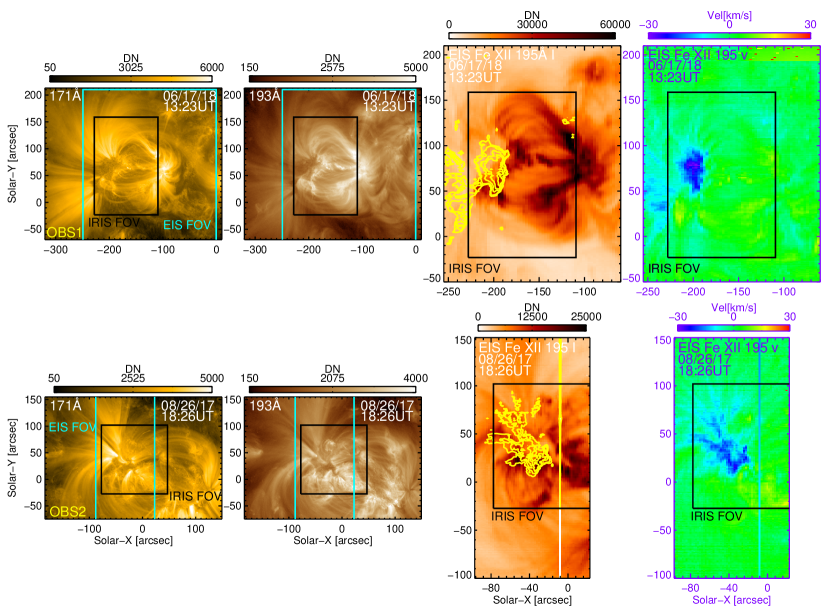
Figure 1.— From left to right: AIA 171 Å and 193 Å images of the two AR observations under study, with the EIS and IRIS FOVs overlaid; intensity and Doppler velocity maps of the EIS Fe XII 195 Å line for OBS1 (top) and OBS2 (bottom).

The AR outflows have often been invoked as a possible source of slow solar wind (e.g. Sakao et al., 2007). EIS observations, combined with in-situ measurements, have shown that the outflows have a slow-wind plasma composition, in agreement with this hypothesis (e.g. Brooks & Warren, 2011, 2012; Brooks et al., 2015). Recent high-resolution observations from Hi-C 2.1 (Rachmeler et al., 2019) have also suggested the existence of photospheric and coronal components to the outflows, which may explain the variable composition of the slow wind (Brooks et al., 2020).

Nevertheless, a definitive model to explain how the outflows are driven and connected to the slow wind is still lacking. A popular scenario assumes that interchange reconnection between closed dense AR loops and neighbouring open (or distantly connected) large-scale low-density loops may act as a mechanism for driving the outflows (e.g. Baker et al., 2009; Del Zanna et al., 2011a).

One issue with this picture is that the outflows are not always observed in the vicinity of open field lines (e.g. Culhane et al., 2014), and Boutry et al. (2012) estimated that a significant fraction of the outflows propagate into long loops connected to distant ARs. A solution might be provided by a “two-step” reconnection process (Culhane et al., 2014; Mandrini et al., 2015), where closed loop plasma first travels along long loops and then, in a second step, is released into the open field lines via interchange reconnection.

Alternative scenarios suggest that the outflows are linked to chromospheric jets and spicules, which are heated while propagating into the corona (McIntosh & De Pontieu, 2009; De Pontieu et al., 2009, 2017).

The height at which the outflows are driven, whether in the corona or the lower atmosphere, is still under debate.

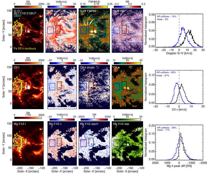
Figure 2.— Top rows (from left to right): total intensity, Doppler shifts, FWHM and RB asymmetry maps, and histograms of Doppler shifts of Si IV in the outflow and moss boxed regions. Middle rows: first and second moments, second moment for single peaked profiles only and third moment of the C II line, and histograms of the second moment in the boxed regions. Bottom rows: Mg II k3 intensity, velocity, k2 peak asymmetry and peak separation, and histograms of the k2 peak asymmetry in the boxed regions. Contours of the EIS Fe XII outflows are also overlaid in yellow. The histograms are normalised by the number of pixels in each box. The percentage of pixels with negative velocity (for Si IV and C II) or positive counts (for Mg II asymmetry) for both moss and outflow regions is also reported in each panel.

Vanninathan et al. (2015) suggested that there was not enough chromospheric jet-like activity or spectral asymmetries in H$\alpha$ to account for a connection with outflows. On the other hand, He et al. (2010) found intermittent upflows in Hinode/XRT images, associated with chromospheric jets observed by Hinode/SOT and blueshifts in the EIS He II line, suggesting a possible chromospheric origin of the outflows.

These previous studies showcase the importance of observing the evolution of the outflows throughout different layers of the solar atmosphere. In this work, we combine EIS observations of coronal outflows with recent spectroscopic observations from IRIS (De Pontieu et al., 2014) at high spatial (0.33–0.4^′′) and spectral ($\approx$ 1.5 km s^-1) resolution. We focus on studying emission from Si IV 1393.75 Å (TR), C II 1335.71 Å (upper chromosphere to TR) and Mg II k 2796.35 Å (mid to upper chromosphere) IRIS lines.

2. Observations

We select two ARs that were simultaneously observed by IRIS and EIS: AR 12713 on 2018-06-17 (OBS1) and AR 12672 on 2017-08-26 (OBS2, Figure 1), using large rasters that covered both the moss and outflows at the edge of the ARs. We selected ARs close to disk center, to minimize possible projection effects (Baker et al., 2017; Ghosh et al., 2019). The IRIS datasets were both dense (slit width =  0.33^′′) 320-step rasters, with exposure times t_exp of 8s and 15s respectively. The EIS OBS1 study was a 87-step raster taken with a raster step of 3^′′, slit width of 2^′′ and t_exp = 40s, while OBS2 was a dense 60-step raster with a raster step of 2^′′ and slit width of 1^′′ and t_exp = 45s.

Figure 1 provides a context view of the observations. The two leftmost panels show the ARs under study as observed by AIA in the 171 Å and 193 Å filters, which in ARs are typically dominated by emission from Fe IX (logT(K) $\approx$ 5.85) and Fe XII (logT(K) $\approx$ 6.2), respectively (O’Dwyer et al., 2010; Martínez-Sykora et al., 2011). The field of view (FOV) of the IRIS and EIS rasters are also overlaid. The third and fourth panels show the intensity and Doppler shifts of the EIS Fe XII 195.12 Å line, which were obtained by performing a single Gaussian fit in each pixel. The Fe XII blueshifts highlight the outflow region, while the bright emission at the footpoints of the hot AR core loops, visible in both the AIA 193 Å and EIS Fe XII images, characterizes the moss.

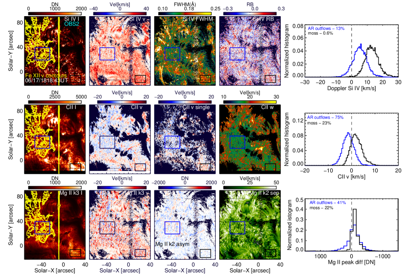
Figure 3.— Same as Fig. 2 for OBS2.

We used IRIS level 2 data that has been corrected for geometrical, flat-field and dark current effects and for the orbital variation of the wavelength array. Further, we use the O I photospheric line to check the absolute wavelength calibration. After summing the O I spectra in a quiet region outside the AR, we estimated that the average velocity shift from the at-rest position of 1355.598 Å was around 0.5 km s^-1.

The EIS data are affected by a series of issues which are described at length in the instrument documentation, and that are carefully taken into account in our analysis. Given the lack of reference photospheric lines to perform an absolute wavelength calibration, the uncertainty in the EIS Doppler shift velocities is usually estimated to be at best $\approx$ 5 km s^-1 (e.g. Young et al., 2012).

To co-align the IRIS and EIS spectroscopic observations, we first compared the SJI 1330 Å  (logT(K) $\approx$ 4.3, De Pontieu et al., 2014) and AIA 1700 Å  (logT(K) $\approx$ 4.2, Simões et al., 2019) images, which are dominated by plasma formed at similar temperatures. The EIS images formed in the He II 256 Å line (logT(K) $\approx$ 4.7) were also co-aligned to AIA 304 Å images, which are dominated by emission from He II (O’Dwyer et al., 2010; Martínez-Sykora et al., 2011). To co-align all the images we used standard cross-correlation routines available in SolarSoft, and also verified the alignment by eye. Using these different methods we estimate a co-alignment uncertainty between IRIS and EIS of $\approx$ 4^′′, which is reasonable considering that the full-width half maximum (FWHM) of the EIS point-spread-function is $\approx$ 3^′′.

2.1. IRIS observations of outflows

In this Section, we focus on observing the spectral features of the IRIS lines in the region underneath the coronal outflows. Figures 2 and 3 provide an overview of the IRIS observations in Si IV (top), C II (middle) and Mg II (bottom) for OBS1 and 2 respectively. The first row shows total intensity, Doppler shift, and FWHM of the Si IV line, assuming a single Gaussian fit, as well as a red-blue (RB) asymmetry map, which was calculated using the algorithm described in Tian et al. (2011) with a $\pm$ 40 km s^-1 velocity interval and a 5 km s^-1 bin. Zero-th (intensity), first (velocity) and second (standard deviation, expressed in km s^-1) moments of the C II line are shown in the second row. A map of first moments, only for profiles which are identified as single peaked, is also shown in the third panel of the second row. Being optically thick, the C II line has a complex formation and can exhibit two or more peaks. We identified the single peaked profiles using the method described in Rathore et al. (2015). The bottom rows of Figs. 2 and 3 show the Mg II 2796 Å line k3 (line core) intensity and velocity, the k2 peak asymmetry (difference between the intensity of the red and blue k2 peaks) and peak separation (difference between the wavelengths of the red and blue k2 peaks, expressed as velocity). The k3 Doppler shifts provide velocity diagnostics in the upper chromosphere, where the line core is formed, while the k2 asymmetry and separation have been shown to provide good diagnostics of flows and velocity gradients (Leenaarts et al., 2013). In particular, a positive/negative k2 asymmetry is typically indicative of up/downflows (because it is caused by increased absorption in the blue/red wavelengths). The contours of the Fe XII outflows are also overlaid in yellow. Finally, each row includes a normalised histogram of Doppler velocities (for Si IV and C II, with bin of 5 km $s^{-1}$) or k2 asymmetries (for Mg II, with a bin of 100 DN) inside the two boxes overlaid in the respective variable maps (black and blue boxes for moss and outflow regions respectively). The percentage of pixels with negative velocity (for Si IV and C II) or positive counts (for Mg II) are also reported in each panel for both moss and outflow regions. Further, we calculated the percentage of pixels taking into account the estimated error on our velocities (0.5 km s^-1) by setting the threshold velocity to 0.5 and -0.5 km s^-1. The percentages of Si IV upflows and their associated range of values taking into account this velocity uncertainty are: 14.4$\%$ (12–17$\%$) in the outflows and 3.3$\%$ (3.1–3.7$\%$) in the moss for OBS1, and 12.9$\%$ (11–15$\%$) in the outflows and 0.6$\%$ (0.5–0.7$\%$) in the moss for OBS2. These values suggest that the fraction of pixels showing Si IV upflows in the outflow region is significantly higher (at least 4 times higher in OBS1) than that in the moss.

Figures 2 and 3 show some clear features that distinguish the outflow from the moss region: (1) the average distribution of Si IV Doppler shift is shifted towards the blue in the outflow regions, with an average value of $\mu_{out}$ $\approx$ 5.4–5.6 km s^-1 and standard deviation $\sigma_{out}$ $\approx$ 4.8–4.6 km s^-1 for OBS1 and 2 (compared to the moss values of $\mu_{moss}$ $\approx$ 12.6–13.3 km s^-1 and $\sigma_{moss}$ $\approx$ 7.4–4.6 km s^-1 respectively); (2) Si IV upflows up to $\approx$ -10 km s^-1 are observed in the outflow region but not in the moss, where the line is consistently redshifted; (3) a similar trend is visible in C II, with the difference that the velocity distributions in outflows and moss regions are both shifted towards the blue compared to those of Si IV. The values for C II are: $\mu_{out}$ $\approx$ -1.4 and -1.1 km s^-1, $\sigma_{out}$ $\approx$ 2.3 and 2.4  km s^-1, in contrast to $\mu_{moss}$ $\approx$ 2.6 and 2.4 km s^-1, $\sigma_{moss}$ $\approx$ 3.5 and 2.5 km s^-1 for OBS1 and OBS2 respectively; (4) we observe a higher concentration of Mg II profiles with positive k2 asymmetry (i.e. upflows) in the outflows than in the moss region.

The O I 1355.598 Å line also appears to be more blueshifted in the outflows compared to the moss. However, since the line is faint, the Doppler shift measurements can be uncertain. No peculiar features are observed in the Mg II triplet lines in the outflow regions.

2.2. Combining IRIS and EIS observations for OBS1

Figure 4 shows an overview of the EIS lines (OBS1) formed over a broad range of temperatures. The O V 192.9 Å line is close in wavelength to the hot Fe XI 192.83 Å and Ca XVII 192.82 Å lines (Young et al., 2007), but can be usually reliably resolved using a multi-Gaussian fit. We note that the unblended O V line at 248.46 Å was not included in this observation program, while other oxygen TR lines such as O IV and O VI are too faint. The Fe VIII 185.21 Å line is also blended with the hotter Ni XVI 185.23 Å line which is mostly visible in the AR cores (Young et al., 2007). The Fe VIII line is formed at the same temperature as the Si VII 275.75 Å line, which is largely free of blends and also shown in Fig. 4. Both Fe VIII and Si VII show some faint blueshifted emission in the outflow region.

The strong Fe XII 195.12 Å line is self-blended with a Fe XII transition at 195.18 Å that can become more significant at high densities ($>$ 10¹⁰ cm^-3, Del Zanna & Mason, 2005). The weaker Fe XII 192.39 Å and the Fe XIII 202.04 Å (logT(K) $\approx$ 6.25) lines are also included in this study and they are both mostly free of blends (Young et al., 2007; Del Zanna et al., 2011b).

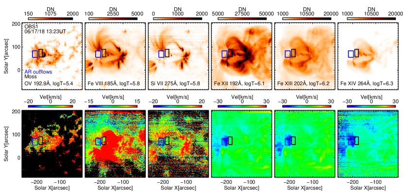
Figure 4.— Intensity (top) and Doppler shift (bottom) maps of EIS lines formed at different temperatures for OBS1. The outflows and moss boxed regions (same as those in Fig. 2) are overlaid on each panel.

Figure 5 summarizes the average velocities observed by EIS and IRIS in the moss and outflows regions of OBS1. These values have been obtained by averaging the velocity inside the boxes highlighted in Fig. 2 and Fig. 4. For Fe XII, we take the Doppler shifts of the 192.39 Å line, but also include the values obtained for the 195.12 Å line (triangles) for reference. For the Mg II line we used the k3 Doppler shift.

Figure 5 shows a similar trend of increasing blueshifts with temperature for the EIS hotter lines (logT(K) $\approx$ 5.8–6.3, e.g. Si VII–Fe XIV),

as that reported in Figure 3 of Del Zanna (2008). The cooler EIS and IRIS lines (logT(K) $\approx$ 4–5.4) show that the trend is almost inverted in the lower atmosphere, with the O V, Si IV and Mg II lines being on average redshifted, while interestingly the C II line is slightly blueshifted.

For comparison, Figure 5 also shows the Doppler shift trend for the moss region. The blueshifts are consistently smaller while the redshifts are larger in the moss as compared to the outflow region, although the trend of Doppler shifts vs temperature appears to be similar in the two regions.

It is important to note that Figs. 2 and 3 reveal a more complicated picture than that suggested by the averaged trend of Fig. 5, with the presence of small-scale TR and chromospheric upflows in the high-resolution IRIS data.

3. Discussion and conclusions

IRIS TR and chromospheric observations offer a unique view of the lower atmospheric counterpart of the long-studied AR outflows at very high spatial and spectral resolution. We analysed two observations of AR outflows with IRIS and EIS and found that:

• IRIS reveals that the low atmosphere underneath the coronal outflows appears to be highly structured, with a percentage of $\approx$ 13$\%$ pixels showing small scale upflows in Si IV (up to $\approx$ -10 km s^-1), as compared to 3 $\%$ or less in the moss.

• The Si IV TR line is also on average less redshifted in the outflow region ($\approx$ 5.5 km s^-1) than in the moss ($\approx$ 13 km s^-1). The average Si IV redshift in the outflows is also lower than typical QS values (7.5 km s^-1 from an IRIS sample observation, in agreement with measurements from previous instruments, e.g. Doschek et al. 1976; Brekke et al. 1997). In contrast with the moss region, where the profiles show some red asymmetry, the Si IV spectra show no asymmetry or a modest blue asymmetry in the outflow region.

• The Mg II k2 asymmetry maps show more profiles with a higher red peak in the outflow region than in the moss. This can be interpreted as evidence of upflows (i.e., more absorption in the blue wing, Leenaarts et al., 2013; Sainz Dalda et al., 2019). The average k3 velocities in the outflow region are also smaller ($\approx$ 2 km s^-1) compared to the moss ($\approx$ 3 km s^-1) .

• While being redshifted in the moss ($\approx$ 2.5 km s^-1), the C II line is on average sligthly blueshifted ($\approx$ -1.1–1.5 km s^-1) in the outflow region. As a comparison, Rathore et al. (2015) previously reported median values of C II Doppler shifts (calculated assuming Gaussian fits) of $\approx$ 0 km s^-1 in the QS network and plage, and $\approx$-2.3 km s^-1 in the QS internetwork.

Our findings show that there is a clear correlation between the chromosphere and TR observed by IRIS and the coronal AR outflows observed by EIS. Such correlation has never been shown before and is surprising given previous work which found no connection between chromospheric activity and coronal outflows using H$\alpha$ data from IBIS (Vanninathan et al., 2015). However, it is not clear why such a connection should make itself visible through the asymmetry of an optically thick line with a complex formation mechanism like H$\alpha$. Our results suggest that the restricted focus on blue-ward asymmetries in the H$\alpha$ line misses the actual association between chromospheric and TR signals and coronal outflows.

There are no models that can currently explain the regional differences of chromospheric and TR properties between outflow regions and moss or QS. We cannot determine from these preliminary studies whether this association occurs because the mechanism that drives outflows occurs at these low heights, or because the outflow regions are actually driven in the larger coronal volume but have a different coronal thermodynamic environment that indirectly affects the lower-lying regions, due for example to the fact that AR outflows may be connected to open field regions, as it is commonly assumed. Comparisons between the closed field regions in QS and open field regions in coronal holes (CHs) have reported subtle differences with CH network showing somewhat less redshifted profiles in low TR spectral lines (McIntosh et al., 2011), similarly to what we observe here. However, from a preliminary analysis, other properties such as the Si IV line widths and Mg II spectral properties seem to behave differently in CHs and AR outflows.

Previous work has demonstrated that the dynamics of the upper chromosphere and low TR in plage are strongly affected by processes that are driven from the lower atmosphere. For instance, magneto-acoustic shocks are ubiquitous in plage (Hansteen et al., 2006) and have a major impact on the properties of the Mg II  h&k, C II and Si IV lines (e.g., De Pontieu et al., 2015). Similarly, the disk counterparts of type II spicules lead to sudden blueshifted excursions in chromospheric lines and broadened linear features in Si IV  (Tian et al., 2014; Rouppe van der Voort et al., 2015; De Pontieu et al., 2017). Perhaps the modification of these phenomena in the open fields of outflow regions plays a role in explaining our results? For example, it is well known that spicules are taller and have different dynamical properties in open fields (Beckers, 1968). There are also suggestions from numerical models that the magnetic topology of a region plays an important role and that TR emission and flow patterns are significantly different in short, low-lying loops (that are not connected to the corona), from those in longer, higher coronal loops, with the height of heating determining the strength of TR redshifts and/or blueshifts (Guerreiro et al., 2013; Hansteen et al., 2014). Perhaps the observed differences in TR properties are related to a different proportion of low-lying to higher loops or that heating occurs at a different height in AR outflow sites compared to moss regions (or CHs)?

More extensive statistical studies and numerical modeling are clearly required to settle these issues. The exact impact of the open fields on the upper chromosphere and low TR thus remains uncertain.

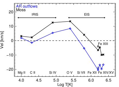
Figure 5.— Velocity vs temperature in outflows and moss for different EIS and IRIS lines.

Nevertheless, our work strongly suggests that the low atmosphere and the corona should not be treated as separate environments, but rather that the processes occurring throughout different layers of the solar atmosphere are likely connected, and should be addressed together by a global model. This is also supported by the fact that the leading theories to explain the first ionization potential (FIP) effect are based on the idea that the FIP fractionation most likely takes place in the upper chromosphere (e.g. Laming, 2015; Laming et al., 2019).

So how do our IRIS observations fit within the context of the most recent models of outflows? These are based on interchange reconnection between closed and open field lines. Modelling by Bradshaw et al. (2011) (in 1D) and Harra et al. (2012) (in 3D) has demonstrated that coronal outflows could be explained as pressure-driven flows following reconnection between closed and open field lines. However, both papers mostly focused on the synthesis of hotter emission observed by EIS. Our work suggests that future outflow models need to include a proper treatment of the chromosphere and TR (i.e., including optically thick radiative losses, convective motions, magneto-acoustic shocks, and spicules) to explain both EIS and IRIS observations. Such models may be able to elucidate whether waves and heating associated with spicules (De Pontieu et al., 2017) plays any role in outflow regions, possibly related to differences in the underlying photospheric magnetic fields (Samanta et al., 2019).

Our work demonstrates that to understand the origin of AR outflows it is crucial to follow the plasma dynamics through different layers of the atmosphere. Our results raise several unsolved questions about the nature of outflow regions and provide a challenge to previous and future models on outflows. Coordinated observations between IRIS and high-sensitivity radio observatories, such as the Jansky Very Large Array, as well as the recent Parker Solar Probe and Solar Orbiter missions, will be key to obtain a more complete picture of the outflow regions and their connection to the solar wind.

References

- Baker et al. (2017) Baker, D., Janvier, M., Démoulin, P., & Mand rini, C. H. 2017, Sol. Phys., 292, 46
- Baker et al. (2009) Baker, D., van Driel-Gesztelyi, L., Mandrini, C. H., Démoulin, P., & Murray, M. J. 2009, ApJ, 705, 926
- Beckers (1968) Beckers, J. M. 1968, Sol. Phys., 3, 367
- Boutry et al. (2012) Boutry, C., Buchlin, E., Vial, J. C., & Régnier, S. 2012, ApJ, 752, 13
- Bradshaw et al. (2011) Bradshaw, S. J., Aulanier, G., & Del Zanna, G. 2011, ApJ, 743, 66
- Brekke et al. (1997) Brekke, P., Hassler, D. M., & Wilhelm, K. 1997, Sol. Phys., 175, 349
- Brooks et al. (2015) Brooks, D. H., Ugarte-Urra, I., & Warren, H. P. 2015, Nature Communications, 6, 5947
- Brooks & Warren (2011) Brooks, D. H., & Warren, H. P. 2011, ApJ, 727, L13
- Brooks & Warren (2012) —. 2012, ApJ, 760, L5
- Brooks et al. (2020) Brooks, D. H., Winebarger, A. R., Savage, S., et al. 2020, ApJ, 894, 144
- Bryans et al. (2010) Bryans, P., Young, P. R., & Doschek, G. A. 2010, ApJ, 715, 1012
- Culhane et al. (2007) Culhane, J. L., Harra, L. K., James, A. M., et al. 2007, Sol. Phys., 243, 19
- Culhane et al. (2014) Culhane, J. L., Brooks, D. H., van Driel-Gesztelyi, L., et al. 2014, Sol. Phys., 289, 3799
- De Pontieu et al. (2017) De Pontieu, B., De Moortel, I., Martinez-Sykora, J., & McIntosh, S. W. 2017, ApJ, 845, L18
- De Pontieu et al. (2015) De Pontieu, B., McIntosh, S., Martinez-Sykora, J., Peter, H., & Pereira, T. M. D. 2015, ApJ, 799, L12
- De Pontieu et al. (2009) De Pontieu, B., McIntosh, S. W., Hansteen, V. H., & Schrijver, C. J. 2009, ApJ, 701, L1
- De Pontieu et al. (2014) De Pontieu, B., Title, A. M., Lemen, J. R., et al. 2014, Sol. Phys., 289, 2733
- Del Zanna (2008) Del Zanna, G. 2008, A&A, 481, L49
- Del Zanna et al. (2011a) Del Zanna, G., Aulanier, G., Klein, K. L., & Török, T. 2011a, A&A, 526, A137
- Del Zanna & Mason (2005) Del Zanna, G., & Mason, H. E. 2005, A&A, 433, 731
- Del Zanna et al. (2011b) Del Zanna, G., Mitra-Kraev, U., Bradshaw, S. J., Mason, H. E., & Asai, A. 2011b, A&A, 526, A1
- Doschek et al. (1976) Doschek, G. A., Feldman, U., & Bohlin, J. D. 1976, ApJ, 205, L177
- Doschek et al. (2008) Doschek, G. A., Warren, H. P., Mariska, J. T., et al. 2008, ApJ, 686, 1362
- Ghosh et al. (2019) Ghosh, A., Klimchuk, J. A., & Tripathi, D. 2019, ApJ, 886, 46
- Guerreiro et al. (2013) Guerreiro, N., Hansteen, V., & De Pontieu, B. 2013, ApJ, 769, 47
- Hansteen et al. (2014) Hansteen, V., De Pontieu, B., Carlsson, M., et al. 2014, Science, 346, 1255757
- Hansteen et al. (2006) Hansteen, V. H., De Pontieu, B., Rouppe van der Voort, L., van Noort, M., & Carlsson, M. 2006, ApJ, 647, L73
- Harra et al. (2012) Harra, L. K., Archontis, V., Pedram, E., et al. 2012, Sol. Phys., 278, 47
- Harra et al. (2008) Harra, L. K., Sakao, T., Mandrini, C. H., et al. 2008, ApJ, 676, L147
- He et al. (2010) He, J. S., Marsch, E., Tu, C. Y., Guo, L. J., & Tian, H. 2010, A&A, 516, A14
- Hinode Review Team et al. (2019) Hinode Review Team, Al-Janabi, K., Antolin, P., et al. 2019, PASJ, 71, R1
- Laming (2015) Laming, J. M. 2015, Living Reviews in Solar Physics, 12, 2
- Laming et al. (2019) Laming, J. M., Vourlidas, A., Korendyke, C., et al. 2019, ApJ, 879, 124
- Leenaarts et al. (2013) Leenaarts, J., Pereira, T. M. D., Carlsson, M., Uitenbroek, H., & De Pontieu, B. 2013, ApJ, 772, 90
- Mandrini et al. (2015) Mandrini, C. H., Baker, D., Démoulin, P., et al. 2015, ApJ, 809, 73
- Marsch et al. (2004) Marsch, E., Wiegelmann, T., & Xia, L. D. 2004, A&A, 428, 629
- Martínez-Sykora et al. (2011) Martínez-Sykora, J., De Pontieu, B., Testa, P., & Hansteen, V. 2011, ApJ, 743, 23
- McIntosh & De Pontieu (2009) McIntosh, S. W., & De Pontieu, B. 2009, ApJ, 706, L80
- McIntosh et al. (2011) McIntosh, S. W., Leamon, R. J., & De Pontieu, B. 2011, ApJ, 727, 7
- O’Dwyer et al. (2010) O’Dwyer, B., Del Zanna, G., Mason, H. E., Weber, M. A., & Tripathi, D. 2010, A&A, 521, A21
- Rachmeler et al. (2019) Rachmeler, L. A., Winebarger, A. R., Savage, S. L., et al. 2019, Sol. Phys., 294, 174
- Rathore et al. (2015) Rathore, B., Pereira, T. M. D., Carlsson, M., & De Pontieu, B. 2015, ApJ, 814, 70
- Rouppe van der Voort et al. (2015) Rouppe van der Voort, L., De Pontieu, B., Pereira, T. M. D., Carlsson, M., & Hansteen, V. 2015, ApJ, 799, L3
- Sainz Dalda et al. (2019) Sainz Dalda, A., de la Cruz Rodríguez, J., De Pontieu, B., & Gošić, M. 2019, ApJ, 875, L18
- Sakao et al. (2007) Sakao, T., Kano, R., Narukage, N., et al. 2007, Science, 318, 1585
- Samanta et al. (2019) Samanta, T., Tian, H., Yurchyshyn, V., et al. 2019, Science, 366, 890
- Simões et al. (2019) Simões, P. J. A., Reid, H. A. S., Milligan, R. O., & Fletcher, L. 2019, ApJ, 870, 114
- Tian et al. (2011) Tian, H., McIntosh, S. W., De Pontieu, B., et al. 2011, ApJ, 738, 18
- Tian et al. (2014) Tian, H., DeLuca, E. E., Cranmer, S. R., et al. 2014, Science, 346, 1255711
- Vanninathan et al. (2015) Vanninathan, K., Madjarska, M. S., Galsgaard, K., Huang, Z., & Doyle, J. G. 2015, A&A, 584, A38
- Young et al. (2012) Young, P. R., O’Dwyer, B., & Mason, H. E. 2012, ApJ, 744, 14
- Young et al. (2007) Young, P. R., Del Zanna, G., Mason, H. E., et al. 2007, PASJ, 59, S857